2 Problem description

Formally, the JSMS can be defined as follows. There exist a set of n jobs {J ₁, … , J _n } and a set of m resources or machines {R ₁, … , R _m }.

Each job J _i consists of a sequence of T tasks $$(\theta _{{i1}} ,\,\!\ldots\!,\,\theta _{{iT_{i} }} )$$ . Each task θ _il has a single machine requirement $$R_{{\theta _{{il}} }} $$ and a start time $$st_{{\theta _{{il}} }} $$ to be determined. The main difference with the traditional JSP is that each machine can work at different speeds. Thus, each task θ _il is associated to different durations ( $$p_{{\theta _{{il1}} }} ,\,p_{{\theta _{{il2}} }} ,\,\!\ldots\!,\,p_{{\theta _{{ilp}} }} $$ ) and has different energy consumptions $$e_{{\theta _{{il1}} }} ,\,e_{{\theta _{{il2}} }} ,\!\,\ldots\!,\,e_{{\theta _{{ilp}} }} $$ depending on the machine in which it is executed.

In general, if the speed of a machine is high, the energy consumption increases, but the processing time of the task decreases, meanwhile if the speed is low, the energy consumption decreases and the processing time increases. For simplicity and without loss of generality, we consider three different energy consumptions and processing times for each task. The original processing time of each task is assigned to an energy consumption of the regular speed. If the processing time of a task is increased to 70%, the energy consumption is reduced to 20% (low speed). However, if the processing time of a task is reduced to 30%, the energy consumption is increased to 20% (high speed). Depending on the specific problem, this curve can vary, and therefore the proportion between processing time and energy consumption can significantly change.

A feasible schedule is a complete assignment of starting times to tasks that satisfies the following constraints: (i) the tasks of each job are sequentially scheduled, (ii) each machine can process at most one task at any time, (iii) no preemption is allowed. The objective is to find a feasible schedule that minimizes the completion time of all the tasks and the energy used.

3 Energy-efficiency

Statistical data in 2009 showed that the Germany industrial sector was responsible for ~47% of the total national electricity consumption, and the corresponding amount of CO₂ emissions generated by this consumption summed up to 18–20% (http://www.bmwi.de/EN/root.html). Thus, manufacturing companies are responsible of an important percentage of the environmental outcome and are forced to have manufacturing systems that demonstrate major potential to reduce environmental impacts (Duflou et al., Reference Duflou, Sutherland, Dornfeld, Herrmann, Jeswiet, Kara, Hauschild and Kellens2012).

Recently, there has been growing interest in the development of energy savings due to a sequence of serious environmental impacts and rising energy costs. Research on minimizing the energy consumption of manufacturing systems has focused on three perspectives: the machine level, the product level, and the manufacturing system level. From the machine-level perspective, developing and designing more energy-efficient machines and equipment to reduce the power and energy demands of machine components is an important strategic target for manufacturing companies (Li et al., Reference Li, Zein, Kara and Herrmann2011; Neugebauer et al., Reference Neugebauer, Wabner, Rentzsch and Ihlenfeldt2011). Unfortunately, previous studies show that the share of energy demand for removal of metal material compared with the share of energy needed to support various functions of manufacturing systems is quite small (less than 30%) of total energy consumption (Dahmus & Gutowski, Reference Dahmus and Gutowski2004). From the product-level perspective, modeling embodied product energy framework based on a product design viewpoint for energy reduction approach is beneficial to support the improvements of product design and operational decisions (Seow & Rahimifard, Reference Seow and Rahimifard2011; Weinert et al., Reference Weinert, Chiotellis and Seliger2011). It requires strong commercial simulation software to facilitate the analysis and evaluation of the embodied product energy. The results cannot be applied easily in most manufacturing companies, especially in small- and medium-sized enterprises due to the enormous financial investments required. From the manufacturing system-level perspective, thanks to decision models that support energy savings, it is feasible to achieve a significant reduction in energy consumption in manufacturing applications. In the specialized literature about production scheduling, the key production objectives for production decision models, such as cost, time and quality have been widely discussed. However, decreasing energy consumption in manufacturing systems through production scheduling has been rather limited.

One of the most well-known research works is the work of Mouzon et al. (Reference Mouzon, Yildirim and Twomey2007), who developed several algorithms and a multiple objective mathematical programming model to investigate the problem of scheduling jobs on a single CNC machine in order to reduce energy consumption and total completion time. They pointed out that there was a significant amount of energy savings when non-bottleneck machines were turned off until needed; the relevant share of savings in total energy consumption could add up to 80%. They also reported that the inter-arrivals would be forecasted and therefore more energy-efficient dispatching rules could be adopted for scheduling. In further research, Mouzon and Yildirim (Reference Mouzon and Yildirim2008) proposed a greedy randomized adaptive search algorithm to solve a multi-objective optimization schedule that minimized the total energy consumption and the total tardiness on a machine. Fang et al. (Reference Fang, Uhan, Zhao and Sutherland2011) provided a new mixed-integer linear programming model for scheduling a classical flow shop that combined the peak total power consumption and the associated carbon footprint with the makespan. Yan and Li (Reference Yan and Li2013) presented a multi-objective optimization approach based on weighted gray relational analysis and response surface methodology. Bruzzone et al. (Reference Bruzzone, Anghinolfi, Paolucci and Tonelli2012) presented an energy-aware scheduling algorithm based on a mixed-integer programming formulation to realize energy savings for a given flexible flow shop that was required to keep fixed original job assignment and sequencing. Although the majority of the research on production scheduling has not considered energy-saving strategies completely, the efforts mentioned above provide a starting point for exploring an energy-aware schedule optimization from the viewpoint of energy consumption.

4 Modeling and solving a job-shop scheduling problem with different speed machine as a genetic algorithm

The most natural way to solve a traditional JSP is to represent all variables and constraints related to jobs, tasks and machines (Garrido et al., Reference Garrido, Salido, Barber and Lopez2000; Huang & Liao, Reference Huang and Liao2008) in order to be solved by a sound and completed search technique. The traditional objectives are to obtain solutions that minimize the typical objective functions presented in the literature (makespan, tardiness, completion time, etc.). It is well-known that this problem is NP-hard, so that optimal solutions can only be achieved for small instances. However, few techniques have been developed to minimize energy consumptions in these problems. Only in the last few years, some researchers have focused their attention to the machine level in order to solve the scheduling problem by minimizing the energy consumption (Dai et al., Reference Dai, Tang, Giret, Salido and Li2013). This requirement increases the complexity of the problem so it is not possible to obtain optimal solutions. This problem called JSMS must be solved by heuristic and metaheuristic techniques in order to obtain optimized solutions, mainly in large instances. To this end, in this paper we develop a GA to solve the JSMS. In Section 5, it can be observed that powerful commercial techniques were not able to solve large instances in a reasonable time; meanwhile small instances are solved by both techniques with similar solution quality.

The approach we propose uses a GA to solve the JSMS. GAs are adaptive methods which may be used to solve optimization problems (Beasley et al., Reference Beasley, Martin and Bull1993). They are based on the genetic process of biological organisms. Over many generations, natural populations evolve according to the principle of natural selection, that is survival of the fittest. At each generation, every new individual (chromosome) corresponds to a solution, which in our case is a schedule for the given JSMS instance. Before a GA can be run, a suitable encoding (or representation) of the problem must be devised. The essence of a GA is to encode a set of parameters (known as genes) and to join them together in order to form a string of values (chromosome). A fitness function is also required, which assigns a figure of merit to each encoded solution. The fitness of an individual depends on its chromosome and is evaluated by the fitness function. During the execution, parents must be selected for reproduction and recombined to generate offspring. Parents are randomly selected from the population, using a scheme which favors fitter individuals. Having selected two parents (Procedure Select—Parents in Algorithm 1, their chromosomes are combined, typically by using crossover and mutation mechanisms to generate better offspring that means better solutions). The process is iterated until a stopping criterion is satisfied.

Algorithm 1 shows the general steps of our GA. All functions are explained in detail in following subsections.

4.1 Chromosome encoding and decoding

In GA, a chromosome represents a solution in the search space. The first step in constructing the GA is to define an appropriate genetic representation (coding). A good representation is crucial because it significantly affects all the subsequent steps of the GA. Many representations for the JSP have been developed.

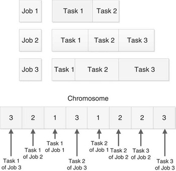
A chromosome is a permutation of the set of operations that represents a tentative ordering to schedule them, each one being represented by its job number. Figure 1 shows an example of a job-shop schedule with three jobs, where job 1 has two tasks, and both jobs 2 and 3 have three tasks. Each number in the chromosome cell (3, 2, 1, 3, 1, 2, 2, 3) represents the job of the task. The first number ‘3’ represents the first task of the job 3. As it was shown in Varela et al. (Reference Varela, Serrano and Sierra2005), this encoding has a number of interesting properties for the classic JSP. For instance a random assignment of values 1, 2 and 3 generates a valid solution.

Figure 1

Codification of a chromosome in a job-shop scheduling problem

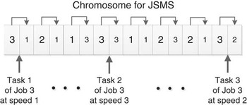
However, in the problem JSMS, the machine speed of each task has to be represented, therefore a new value must be added to each task in order to represent the machine speed. So a valid chromosome is 2n length, where n is the total number of tasks. Figure 2 shows the coding of a chromosome in JSMS. Such coding increases the former coding for adding the speed at which each task is processed. Thus, the first two digits 3 and 1 means that the first task of the job 3 is processed at speed 1. Again, a random assignment of values to tasks and speed generates a valid solution. When the chromosome representation is decoded each task starts as soon as possible following the precedence and machine constraints. With the machine speed representation, the processing time of each task and energy consumption of the machine can be calculated, and therefore the makespan and total energy consumption.

Figure 2

Codification of a chromosome in a job-shop scheduling problem with different speed machine (JSMS)

4.2 Initial population and fitness

As we have pointed out before, each gene represents one task of the problem and the next gene represents the speed at which this task is processed. The position of each task determines its dispatch order, in this genome/solution. The initial chromosomes are obtained by a random permutation of tasks. The machine speed for each gene is also randomly generated among one of the possible speeds. Thus, the initial population is randomly generated to obtain feasible schedules (Procedure Initial—Population in Algorithm 1). According to the instance size, the population is properly tuned.

JSMS can be considered a multi-objective problem due to the fact that the goal is to minimize the makespan and also to minimize the energy consumption. However, both objectives are contrary so that minimize the makespan supposes to increase the speed of machines, and vice versa. Thus, in these problems no single optimal solution exists. Instead, a set of efficient solutions are identified to compose the Pareto front. Diverse techniques have been developed to solve multiple objective optimization problems. One of the most well-known methods for solving multiple objective optimization problems is the Normalized Weighted Additive Utility Function (NWAUF), where multiple objectives are normalized and added to form a utility function. NWAUF has been used widely for multiple objective optimization problems due to its simplicity and natural ability to identify efficient solutions. Let f _ij be the ith objective function value of alternative j. Then, the NWAUF for alternative j with k objectives is defined as

(1) $$U_{j} \, {\equals}\, w_{1} f'_{{1j}} {\plus}w_{2} f'_{{2j}} {\plus}...{\plus}w_{k} f'_{{kj}} $$

where w ₁, w ₂, … , w _k are weights of importance and $f_{{1j}}^{'} ,\,f_{{2j}}^{'} ,\,\!\ldots\!,\,f_{{kj}}^{'} $ are normalized values of f _1j , f _2j , … , f _kj . By normalizing different objectives, all objectives are evaluated in the same scale. Weights show decision maker’s preference for each objective where, $$\mathop{\sum}\nolimits_{i\, {\equals}\, 1}^k w_{i} \, {\equals}\, 1$$ and 0⩽w _i ⩽1 for i=1, … , k. Using this utility function, the multiple objective optimizations can now be solved as a single objective optimization problem.

The definition of fitness function is just the reciprocal of the objective function value. The objective is to find a solution that minimizes the multi-objective makespan and energy consumption. Following NWAUF rules, our fitness function F(i) (2) is a convex combination between the normalized values of makespan and energy consumption of solution i.

(2) $$F(i)\, {\equals}\, \lambda {\times}NormMakespan\,(i){\plus}(1{\minus}\lambda ){\times}NormEnergy\,(i)$$

(3) $$NormMakespan\,(i)\, {\equals}\, {{Makespan\,(i)} \over {MaxMakespan}}$$

(4) $$NormEnergy\,(i)\, {\equals}\, {{SumEnergy\,(i)} \over {MaxEnergy}}$$

where λ∈[0, 1]. NormMakespan (3) is the makespan divided by the maximum makespan value in a GA execution when the λ value is equal to 0 (MaxMakespan). MaxMakespan values can be found in the benchmark section of our Web pageFootnote ¹ . NormEnergy (4) is calculated by summing the energy used in the execution of all the tasks, and then dividing the result by the maximum energy (MaxEnergy). MaxEnergy is the sum of the energy needed to execute all tasks at top speed.

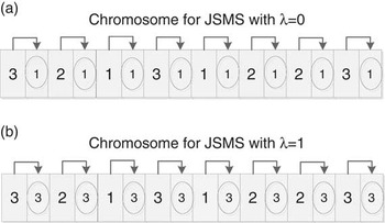
Once the λ parameter is set for the fitness function (2), the initial population can be generated in a specific way. Thus, for λ=0, the objective function is only focused to reduce the energy consumption (F=NormEnergy), so the initial population can be randomly generated to order the tasks, but the corresponding speeds are fixed to the lowest value (see Figure 3a). In the same way, if λ=1, the objective function is only focused to reduce makespan (F=NormMakespan), so the initial population can also be randomly generated to order the tasks, but the corresponding speeds are fixed to the highest value (see Figure 3b). For λ∈]0, 1[, the speed of each task can be appropriately generated.

Figure 3

Initial population for λ=0 and λ=1. JSMS=job-shop scheduling problem with different speed machine

4.3 Crossover operator

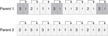
For chromosome mating, our GA uses a (job, energy)-based order crossover. Thus, given two parents, a set of pairs (job, energy) of a random job is selected from the first parent and copied in the same position to the offspring. Afterwards, the set of pairs (job, energy) of the remaining jobs are translated from the second parent to the offspring in the same order (Procedure Crossover in Algorithm 1). We clarify how this technique works in the next example. Let us consider the following two parents (see Figure 4).

Figure 4

Two parents for the crossover operator

If the selected subset of jobs from the first parent just includes the job 3 (dark genes in Figure 4), the generated offspring is showed in Figure 5.

Figure 5

Offspring for the crossover operator

Hence, this technique maintains for a machine a subsequence of operations in the same order as they are in parent 1 and the remaining ones in the same order as they appear in parent 2. The crossover is applied in a dual way, so two parents generate two offspring (parent 1–parent 2) and (parent 2–parent 1). Parent couples are selected shuffling population and choosing each couple two by two, so all individual will be selected but only some couples will be crossed in accordance to crossover probability.

5 Evaluation

In this section, we evaluate the behavior of our GA against a successful and well-known commercial solver IBM ILOG CPLEX CP Optimizer tool 12.5 (CP Optimizer). It is a commercial solver embedding powerful constraint propagation techniques and a self-adapting large neighborhood search method dedicated to scheduling (Laborie, Reference Laborie2009). This solver is expected to be very efficient for a variety of scheduling problems as it is pointed out in IBM (2007), in particular when the cumulative demand for resources exceeds their availability.

These algorithms have been evaluated with extended benchmarks of the typical JSP. The extension has been focused on assigning different speeds and durations to each task (as we pointed out in Section 3). The extension with machines working at different speeds has been implemented considering that each task is executed by a machine and it has different optional modes where each represents the duration of the task and an associated energy consumption (Salido et al., Reference Salido, Escamilla, Barber, Giret, Tang and Dai2013).

To this end, we extend the benchmarks proposed in Agnetis et al. (Reference Agnetis, Flamini, Nicosia and Pacifici2011) and Watson et al. (Reference Watson, Barbulescu, Howe and Whitley1999) because to the best of our knowledge there are no benchmarks for JSPs that incorporate different speeds and energy consumptions. All instances are characterized by the number of jobs (j), the number of machines (m), the maximum number of tasks by job (v _max) and the range of processing times (p). In Agnetis instances, j is set to 3 and these can be represented as m_v _max_p, and the number of operators was not considered in this study, so we fixed it to the number of machines. The population size was set to 200 individual for Agnetis instances and 400 for Watson instances. These values were selected by testing different alternatives and selecting the best results.

We consider two types of instances: small and large Agnetis instances:

• ∙ j=3; m=3, 5, 7; v _max=5, 7, 10; p=[1, 10], [1, 50], [1, 100]

• ∙ j=3; m=3; v _max=20, 25, 30; p=[1, 50], [1, 100], [1, 200]

In Watson instances follow the same characterized, but in this case the variable that changes is the number of jobs (j):

• ∙ j=50, 100, 200; m=20; v _max=20; p=[1, 100]

For each type of instance we work with 10 instances so the results presented in this section are always the averages value. We have modeled the instances to be solved by the CP Optimizer. Moreover, we have extended the original instances as explained in Escamilla et al. (Reference Escamilla, Salido, Giret and Barber2014). These instances can be found in the Web pageFootnote ² .

5.1 Comparative study between CP Optimizer and genetic algorithm

CP and GA techniques try to minimize the multi-objective makespan and energy consumption. The weight of each objective can be changed by λ parameter, following the expression (2). In order to compare both techniques, the validation tests have been executed in an Intel Core2 Quad CPU Q9550, 2.83 GHz and 4 GB RAM computer with Ubuntu 12.04 operating system. The small Agnetis instances were executed during 5 seconds and the large Agnetis and Watson instances had a 100 seconds time-out. The next tables present the most important parameter to be analyzed: λ∈[0, 1] that represents the weight given to makespan and energy consumption, Mk is the makespan, En is the energy consumption, and F is the fitness function. The objective is to obtain the lowest value of F.

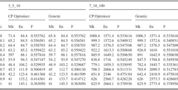
Table 1 shows the results for two small Agnetis instances, the smallest (3_5_10) and the largest (7_10_100) of this group. The results for the instances 3_5_10 show that the F value was equal or almost equal in both CP Optimizer and GA. Furthermore, there were small differences in all λ values for instance 7_10_100. These results show that both algorithms maintained the same behavior for small instances (the difference is in the fourth decimal).

Table 1

Results of small Agnetis instances

Mk=makespan; En=energy consumption; F=fitness function.

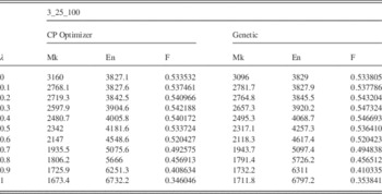
In large Agnetis instances, the results were also similar for all the instances. Table 2 shows the results for the instances 3_25_100 as an example. The difference of F value between CP Optimizer and GA was almost in the third decimal in most cases. It must be taken into account that for λ=0.6 or λ=0.8, the F value of our GA was lower than in CP Optimizer. This is due to the fact that the initial population, for λ=1 is composed of high speed values (3).

Table 2

Results of large Agnetis instances

Mk=makespan; En=energy consumption; F=fitness function.

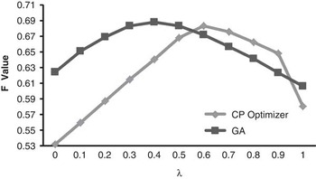
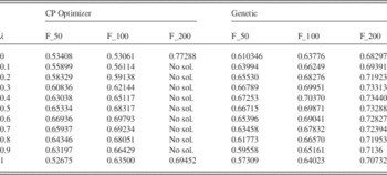
Table 3 shows the F values for Watson instances. In Agnetis instances, the maximum number of operations is 90 in instances 3_30_p. However, in Watson instances, the number of operations is ranged between 1000 (j=50 and v _max=20) and 4000 operations (j=200 and v _max=20). Therefore, Watson instances are much larger than Agnetis instances. It can be observed that both algorithms were able to solve all instances with 50 and 100 jobs. The results for these instances were better for CP Optimizer for λ values <0.6, meanwhile our GA had better results for λ∈[0.6, 0.9[. Figure 6 shows the average F value of 50 and 100 jobs for Watson instances. It can be observed that although both algorithms have similar behavior, GA is mainly focused on minimizing makespan (highest value for λ=0.4) meanwhile CP Optimizer is mainly focused on minimizing energy consumption (highest value for λ=0.6).

Figure 6

Average F value (F_50 and F_100) for Watson instances

Table 3

Results of Watson instances

However, for instances of 200 jobs, CP Optimizer was unable to solve almost all instances ranged for λ∈]0, 1[. This means CP Optimizer is not able to solve large-scale instances in a reasonable time so metaheuristic techniques are needed to obtain optimized solutions in a given time.

6 Conclusions and further works

Many real-world problems can be modeled as a scheduling problem. In this case we are working with an extended version of the classical JSP in which machines can consume different amounts of energy to process tasks at different rates. Each operation has to be executed by one machine and this machine has the possibility to work at different speeds. In this work, we develop a GA to solve the JSMS problem. The representation of energy consumption in the chromosome gives the opportunity to guide the search toward an optimized solution in an efficient way. A comparative study was carried out to analyze the behavior of our GA against a well-known solver: IBM ILOG CPLEX CP Optimizer. The evaluation shows that our GA had a similar behavior than CP Optimizer for small instances. However, for large instances, CP Optimizer was unable to solve them in the given time, meanwhile our GA could solve all instances with the same optimality degree. Thus, our technique can be useful for application in large-scale scheduling problems.

In further works, we aim to add more techniques to GA algorithm such as local search techniques to improve the obtained solutions. It can also be taken into consideration adding a post-process by increasing the speed of the machine that executes tasks in the critical path. Furthermore, we will take into account robustness and energy aware due to the fact that energy-aware solutions can be considered more robust than makespan-optimized solutions (Salido et al., Reference Salido, Escamilla, Barber, Giret, Tang and Dai2013).