


I. INTRODUCTION
The Rietveld refinement is one of the earliest methods of structure characterization based on the whole powder pattern fitting procedure (Rietveld, Reference Rietveld1967). Compared with the other line profile analysis approaches, the major advantage of Rietveld refinement is the estimation of phase fractions in the study of alloys, compounds, or mixture of materials (Attallah et al., Reference Attallah, Zabeen, Cernik and Preuss2009; Ersching et al., Reference Ersching, Campos, Lima, Grandi, Souza and Pizani2010). Today, the newest packages of this method are provided such that the structure and microstructure characters can be simultaneously refined and extracted from the diffraction patterns (Mojtahedi et al., Reference Mojtahedi, Goodarzi, Aboutalebi, Ghaffari and Soleimanian2013). Although in the anisotropic line broadening these packages can well determine the values of crystallite size and mean square of strain corresponding to various hkl reflections, as is known, in only a few Rietveld studies have been evaluated the relation between the anisotropic strain broadening and lattice defects (dislocation characters and planer faults) (Wu et al., Reference Wu, Gray and MacA1998a; Cerny et al., Reference Cerny, Joubert, Latroche, Percheron and Yvon2000). On the other hand, in several recent papers after determining the crystallite size and mean square of strain from Rietveld refinement, the dislocation density of samples has been estimated (Sarkar et al., Reference Sarkar, Mukherjee and Barat2008; Murugesan et al., Reference Murugesan, Kuppusami, Mohandas and Vijayalakshmi2012; Rahaei and Jia, Reference Rahaei and Jia2014; Zhang et al., Reference Zhang, Jiang, Fu, Cai and Ma2015) by using a formula proposed by Williamson and Smallman (Reference Williamson and Smallman1956). The drawback of this equation is that, not only neglecting the effects of slip systems and contrast factor of dislocation, but also considering the contribution of both the size and distortion broadening in dislocation evaluation. However, according to the advanced X-ray diffraction line profile analysis the dislocations can only affect the anisotropic strain broadening and they have no influence on the broadening of size (Ungar et al., Reference Ungar, Leoni and Scardi1999a; Dragomir and Ungar, Reference Dragomir and Ungar2002).
It seems that if, instead of the old X-ray method, the newer theories of line profile analysis are combined with the Rietveld refinement procedure, it can be more accurately studied the influence of structure and microstructure characters on the mechanical, chemical, or physical properties of materials. In this work, the basis of anisotropic strain broadening formulated by Stephens in Rietveld method (Stephens, Reference Stephens1999) is incorporated to the modified form of Caglioti equation proposed by Wu et al. (Reference Wu, Gray and MacA1998a). The result is compared with the relation between the contrast factor of dislocation and fourth-order invariant coefficients, reported by Ungar and Tichy (Reference Ungar and Tichy1999b). This procedure can estimate the fraction of edge/screw dislocation types and dislocation density in cubic system.
In order to check the reliability of the Rietveld method, the X-ray diffraction data were tested for four different samples. The first two materials, prepared by the top-down nanofabrication technique are the mechanical alloying of elemental copper/iron and aluminum powders. The other materials, selected from the bottom-up method of nanoparticle preparation, are the nanocrystalline MgO powder and CdO thin films. Both of them were synthesized by sol–gel method. The crystallite size, dislocation density, and the fraction of edge/screw dislocation types corresponding to these samples were determined by Rietveld refinement. In CdO samples, the behavior of these microstructure parameters was evaluated as a function of annealing temperature. Finally, the results were compared with those achieved by one of the powerful methods of microstructure evaluation, i.e. whole powder pattern modeling (WPPM) procedure (Scardi and Leoni, Reference Scardi and Leoni2002).
II. RELATION BETWEEN THE RIETVELD RESULTS AND DISLOCATION PARAMETERS
The structure and microstructure parameters can be evaluated using the space group, the initial values of lattice parameters and the position of atoms in lattice, corresponding to each phase of tested material as the input values of Rietveld software packages (Rodriguez, Reference Rodriguez1990; Ferrari and Lutterotti, Reference Ferrari and Lutterotti1994). The location as well as the approximate intensity of reflections in the diffraction patterns are estimated from the structure factor of each phase. The width of peak profiles is usually the linear or non-linear combination of the breadth of Lorentzian (H L) and Gaussian (H G) functions. For microstructure determination, by applying the Thompson–Cox–Hastings pseudo-Voigt function, the breadth of peak profiles (H K) is taken from the following equation (Solovyov, Reference Solovyov2000):
 $$\eqalign{H_{\rm K}^5 & = H_{\rm G}^5 + 2.69269H_{\rm G}^4 H_{\rm L} + 2.42843H_{\rm G}^3 H_{\rm L}^2 \cr & \quad + 4.47163H_{\rm G}^2 H_{\rm L}^3 + 0.07842H_{\rm G} H_{\rm L}^4 + H_{\rm L}^5, \ldots}$$
where H G and H L can be determined using Eqs. (2) and (3).
 $$H_{\rm G}^2 = U\tan ^2 \theta + V\tan \theta + W + \displaystyle{{I_{\rm G}} \over {\cos ^2 \theta}}$$
 $$H_{\rm L} = X\tan \theta + \displaystyle{Y \over {\cos \theta}}$$
During the fitting procedure, the values of U, V, W, I G, X, and Y as well as the structure parameters must be refined until minimizing the difference between the calculated and observed patterns. Now the volume (D V) and area (D A) weighed crystallite size can be determined in addition to the apparent size (D) and the mean square of strain 〈e 2〉1/2 by using Eqs. (4)–(7) (Rodriguez, Reference Rodriguez1990):
 $$\eqalign{D_{\rm V} & = \displaystyle{{1080\lambda} \over {\pi ^2}} \cr & \quad \left[ {2(Y - Y_{\rm S} ) + \left[ {(Y - Y_{\rm S} )^2 + \displaystyle{9 \over {\pi ^2 Ln^2 2}}(Z - Z_{\rm S} )} \right]^{1/2}} \right]^{ - 1}}$$
 $$D_{\rm A} = \displaystyle{{180\lambda} \over {\pi ^2}} (Y - Y_{\rm S} )^{ - 1}$$
 $$D = D_{\rm A} + \displaystyle{{(D_{\rm A} D_{\rm V} )^{1/2}} \over 4}$$
 $$\eqalign{\langle e^2 \rangle ^{1/2} & = \displaystyle{1 \over {12}}\left( {\displaystyle{{\pi ^2} \over {360}}} \right) \cr & \quad \left[ {2(X - X_{\rm S} ) + \left[ {(X - X_{\rm S} )^2 + \displaystyle{9 \over {\pi ^2 Ln^2 2}}(U - U_{\rm S} )} \right]^{1/2}} \right]^{ - 1}}$$
where Y S, Z S, X S, and U S are the coefficients corresponding to the peak profiles of instrumental sample.
It should be noted that, since in most of the nanocrystalline materials the density of linear defects is very high, the strain of various hkl reflection has no unique value. In this case, which are named anisotropic strain broadening, U and X parameters in Eqs. (2) and (3) must be changed to U + (1 − ζ 2)σ 2 (M)/M 2 and X + ζσ(M)/M. In cubic crystals, according to the Stephens model, M = h 2 + k 2 + l 2 and σ(M) are obtained from the following equation (Stephens, Reference Stephens1999):
 $$\sigma ^2 (M) = S_{400} (h^4 + k^4 + l^4 ) + S_{220} (h^2 k^2 + h^2 l^2 + k^2 l^2 )$$
in which, S 400, S 220, and ζ, in anisotropic strain broadening, are also the refinable parameters during the fitting procedure.
Moreover, according to Wu et al. (Reference Wu, Gray and MacA1998a, Reference Wu, Kisi and Gray1998b), in the dislocated crystals the relationship between the breadth of Gaussian components and the contrast factor of dislocations
 $(\overline C_{hkl} )$
can be given as:
 $$H_{\rm G}^2 = (U + T\chi )\tan ^2 \theta + V\tan \theta + W + \displaystyle{{I_{\rm G}} \over {\cos ^2 \theta}} $$
where
 $\chi = \overline C_{hkl} b^2 $
, b is the Burgers vector, and T is a parameter related to the refinable anisotropic strain broadening parameters. The relation between Lorentzian component and strain broadening is more complicated and therefore in this research only the Gaussian component was applied. Thus, the following equation can be derived by substituting the new form of U (in anisotropic strain broadening case) into Eq. (9):
 $$\eqalign{T\chi & = T\overline C_{hkl} b^2 = \cr & \quad (1 - \zeta )^2 \displaystyle{{s_{400} (h^4 + k^4 + l^4 ) + s_{220} (h^2 k^2 + h^2 l^2 + k^2 l^2 )} \over {(h^2 + k^2 + l^2 )^2}}} $$
On the other hand, according to Ungar and Tichy (Reference Ungar and Tichy1999b), in cubic crystals the average contrast factor can be expressed as the fourth-order polynomials of hkl indexes:
 $$\overline C_{hkl} = A + BH^2 $$
where
 $$H^2 = \displaystyle{{h^2 k^2 + h^2 l^2 + k^2 l^2} \over {(h^2 + k^2 + l^2 )^2}} $$
The average contrast factor can also be written as the fractions of edge (η e) and screw (η s) dislocation characters as:
 $$\overline C_{hkl} = \eta _{\rm e} \overline C_{hkl,{\rm e}} + \eta _{\rm s} \overline C_{hkl,{\rm s}} = \eta _{\rm e} \overline C_{hkl,{\rm e}} + (1 - \eta _{\rm e} )\overline C_{hkl,{\rm s}} $$
In the above equation,
 $\overline C_{hkl,{\rm e}} $
and
 $\overline C_{hkl,{\rm s}} $
are the average contrast factors corresponding to edge and screw dislocation types, respectively. Combining Eqs. (10) to (13), the following equation is obtained:
 $$\eqalign{& Tb^2 [(\eta _{\rm e} A_{\rm e} + \eta _{\rm s} A_{\rm s} ) + (\eta _{\rm e} B_{\rm e} + \eta _{\rm s} B_{\rm s} )H^2 ] \cr &\quad = (1 - \zeta )^2 [S_{400} + (S_{220} - 2S_{400} )H^2 ]} $$
or
 $$\displaystyle{{\eta _{\rm e} A_{\rm e} + \eta _{\rm S} A_{\rm S}} \over {\eta _{\rm e} B_{\rm e} + \eta _{\rm S} B_{\rm S}}} = \displaystyle{{S_{400}} \over {S_{220} - 2S_{400}}} = K^{\prime}$$
Finally, the fractions of edge dislocation characters can be determined from the refinable parameters S 400 and S 200 as:
 $$\eta _{\rm e} = \displaystyle{{K^{\prime}B_{\rm S} - A_{\rm S}} \over {A_{\rm e} - A_{\rm S} + K^{\prime}(B_{\rm S} - B_{\rm e} )}}$$
In order to determine the dislocation density (ρ), according to the approach proposed by Cerny et al. (Reference Cerny, Joubert, Latroche, Percheron and Yvon2000), the relation between the mean square of strain and density of dislocation is as follows:
 $$\langle e^2 \rangle _{hkl} = \displaystyle{\rho \over 8}\Lambda ^2 (\ln P)\overline C_{hkl} b^2 $$
where
 $$\Lambda = \left( {1 - \displaystyle{\ln (\ln P)\over {4\ln P}}} \right)^{ - 1} $$
and P, which is the dislocation correlation parameter, can be approximately determined from the ratio between the Lorentz (β L) and Gauss (β G) integral breadth:
 $$P \simeq 3(\pi \ln 2)^{ - 1/2} \displaystyle{{\beta _{\rm G}} \over {\beta _{\rm L}}} $$
Now according to Eq. (17), the mean value of dislocation density can be determined from the slop of the plot of 〈e
2〉
hkl
vs.
 $\xi _{hkl} = \Lambda ^2 (\ln P)\overline C_{hkl} b^2 /8$
. It is important to point out that, since the anisotropic microstructure section of Fullprof software has been written on the basis of the Stephens model (Stephens, Reference Stephens1999) and can be completely adopted to all of the above assumptions, in our work, this software was selected from among the various Rietveld packages.
III. TESTING THE FORMULA ON CUBIC NANOMATERILAS
A. Materials preparation
In order to test the procedure explained in the previous section, four different cubic materials were selected. The mechanically alloyed nanocrystalline Fe–Cu (sample S 1) and deformed aluminum powders (sample S 2), were prepared by planetary ball-mill. In sample S 1, the weight fractions of Fe and Cu were equal and the milling time of samples S 1 and S 2 was set to 12 and 48 h, respectively. Further details were reported in our previous works (Mojtahedi et al., Reference Mojtahedi, Goodarzi, Aboutalebi, Ghaffari and Soleimanian2013; Soleimanian and Mojtahedi, Reference Soleimanian and Mojtahedi2015).
The nanoparticle of magnesium oxide (sample S 3) was synthesized using the sol–gel technique. In this process, the sodium hydroxide and magnesium nitrate were used as the starting materials. After preparing the MgO nanopowder, it was annealed in air for 2 h at 600 °C (Soleimanian et al., Reference Soleimanian, Abedi and Aghdaee2015).
The last material, attempted to more systematically explain in this research, is the thin film of cadmium oxide (samples S 4–S 8). To deposit the CdO nanoparticles on the ordinary glass slide substrates, the sol–gel spin coating method was applied. The cadmium acetate, 2-methoxiethanol, and monoethanolamine were used as the source of cadmium, solvent, and stabilizer, respectively. The prepared gel was dropped onto the cleaned substrates, the films were rotated at 1000 rpm for 30 min, and dried at 150 °C. After repeating the spin coating drying cycles, the films were annealed at 300–500 °C in air (Yahia et al., Reference Yahia, Salem, Abd and Yakuphanoglu2013).
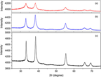
The X-ray diffraction data of samples were measured by Philips PW-1840 and Panalytical X'Pert Pro MPD, diffractometers, using CoK α (λ = 1.789 Å) and CuKα (λ = 1.541 Å) radiations, respectively. The properties of angular range, step size, step counting time, divergence slits, goniometer radius, and detector types are given in Table I. In order to apply the effect of instrumental broadening, the Al2O3 and La2B6 powders with large crystallites and negligible strain were used as the standard samples of first and second diffractometers, respectively. The X-ray diffraction patterns of samples S 4, S 6, and S 8 are shown in Figure 1 [the diffraction profiles of S 1 to S 3 were previously reported in (Mojtahedi et al., Reference Mojtahedi, Goodarzi, Aboutalebi, Ghaffari and Soleimanian2013; Soleimanian and Mojtahedi, Reference Soleimanian and Mojtahedi2015; Soleimanian et al., Reference Soleimanian, Abedi and Aghdaee2015)].
(Color online) The X-ray diffraction patterns of CdO samples annealed at (a) 300, (b) 400 and (c) 500 °C.

Data collection condition.

B. Rietveld refinement procedure
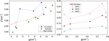
Before any analysis, the behavior of peak profile broadening corresponding to each sample should be investigated. This feature can be observed in the Williamson–Hall plot by analyzing the variation of integral breadth in reciprocal space (β*) vs. the diffraction vector (g) (Williamson and Hall, Reference Williamson and Hall1953). Figure 2 shows the Williamson–Hall plots of Cu (S 1), Al (S 2), MgO (S 3), and CdO (S 4–S 8) phases. As is seen the β* is not a monotonous function of g and the strain anisotropy, observed in the plots must be evaluated vs. linear defects. It should be noted that the Williamson–Hall plot of Fe phase (sample S 1) only has three points and therefore the behavior of line broadening cannot be evaluated for this phase.
(Color online) The Williamson–Hall plots Cu and Mgo phase which show the variation of β* versus g.

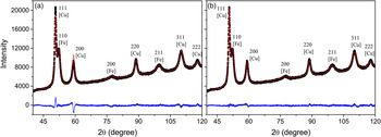
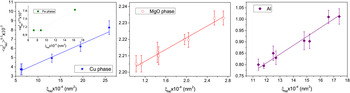
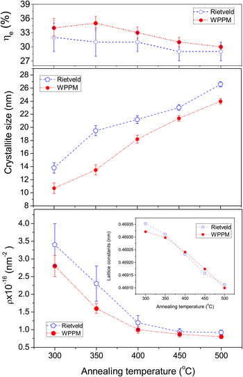
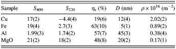
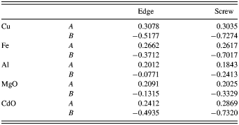
To simultaneously investigate the structure and microstructure properties, the space group, the position of atoms, and the initial values for lattice parameter of each sample were separately used in Fullprof software (Rodriguez, Reference Rodriguez1990). The background parameters, lattice constants, and the coefficients of Eqs. (2) and (3) were then refined and the measured X-ray diffraction patterns were fitted to the calculated one, using Thompson–Cox–Hastings pseudo-Voigt function. But as is shown in Figure 3(a), the quality of fitting is not satisfactory, which is in accordance with the Williamson–Hall plots, the anisotropic strain broadening is presented in the diffraction patterns of all samples. Therefore, according to the Stephans model, in the interface of Fullprof the following sections were consecutively selected: Microstructre/General Strain Formulation/Broadening Model (Quadratic form). S 400, S 220, and ζ were also refined along with the other structure and microstructure parameters. It can be seen in Figure 3(b), after refining the anisotropic parameters (S 400, S 220, and ζ) the fitting quality is significantly improved. Some of the important results are summarized in Tables II and III. Using these values in Eqs. (15) and (16), the fraction of edge dislocation type (η e) was determined (Table III). In order to determine the dislocation density, the contribution of edge and screw dislocation types on the contrast factor of dislocation must be identified. To do this, the elastic constants of our crystals were applied and according to the approach described by Ungar et al. (Reference Ungar, Dragomir, Revesz and Borbely1999c), the values of A e, B e, A s, and B s were determined (Table IV). The details of this procedure are not provided here (see Ungar et al., Reference Ungar, Dragomir, Revesz and Borbely1999c). These values and η e were used in Eqs. (11) and (13) and the contrast factor of each reflection was estimated. On the other hand, the dislocation correlation parameter (P) and also the values of Λ were calculated by Eqs. (18) and (19). Finally, by linear fitting to the plots of 〈e 2〉 hkl as a function of ξ hkl , the dislocation density of the correspond samples was determined (Figure 4). For better understanding, the parameters used in the above procedure (briefly only the values of Cu phase) are arranged in Table V. The results of samples S 1 to S 3 are added to Table III. The behavior of microstructure parameters corresponding to CdO films (samples S 4 to S 8) are also shown in Figure 5. As is seen in these plots, with the increase of annealing temperature from 300 to 500 °C, the values of crystallite size and lattice constant more or less linearly increase and decrease from 13.8(8) to 26.6(4) and 0.469 35(3) to 0.469 11(2), respectively. It can also be observed that the dislocation density quadratically decreases from 3.4(6) to 30(2) and the fraction of edge dislocation type only fluctuates from 32(3) to 29(2)%. The CIF formats of the Rietveld refinement procedure corresponding to four different sample types are available in the Supplementary materials.
(Color online) The measured and calculated diffraction patterns of sample S 1 by assuming (a) The broadening of reflection is isotrop. (b) The broadening of reflection is anisotrop.

(Color online) The variations of 〈e 2〉 hkl versus ξ hkl corresponding to Cu, Fe and Mgo phases.

(Color online) Comparison between the behavior of microstructure parameters corresponding to CdO films, extracted by Rietveld and WPPM methods.

Structure parameters of samples S 1, S 2, and S 3 determined from the Rietveld procedure.

Microstructure parameters of samples S 1 and S 2, determined from the Rietveld refinement procedure.

Parameters of A and B of edge and screw dislocation corresponding to Cu, Fe, Al, MgO, and CdO crystals.

Values of Bragg position, β
G, β
L, P,
 $\langle e^2 \rangle _{hkl}^{1/2} $
, and ξ
hkl
corresponding to Cu phase derived from the Rietveld refinement.

C. Comparison between the results of Rietveld and WPPM
In the next step, the dislocation results of the Rietveld procedure were compared with those extracted from the WPPM. In the WPPM method, the crystallite size, size distribution behavior, dislocation density (ρ), outer cut-off radius of dislocation (R e), and the fraction of edge dislocation characters (η e) can be directly extracted from the diffraction patterns without using any mathematical peak shape function like Voigt or pseudo-Voigt. The theory of the WPPM procedure has been fully described in (Scardi and Leoni, Reference Scardi and Leoni2001, Reference Scardi and Leoni2002); therefore, is not repeated in this study. In this method, by combining the theory of Warren and Averbach (Reference Warren and Averbach1950) with that proposed by Wilkens (Reference Wilkens1976), the Fourier coefficients of simulated intensity profiles can be written in terms of the multiplication of Fourier size and Fourier distortion. Since in most of the conditions, the behavior of distribution function can be described by Lognormal function, the size of Fourier coefficient can be written in terms of Lognormal mean (μ), and Lognormal variance (σ) (Scardi and Leoni, Reference Scardi and Leoni2001). Moreover, the values of contrast factor corresponding to hkl reflections are evaluated using Eq. (13) and refining the values of η e as implemented in PM2 K software (Leoni et al., Reference Leoni, Confente and Scardi2006).
For samples S 1 to S 8, using the PM2K software, the simulated patterns were compared with the measured one and the background coefficients, lattice constants, Lognormal mean, Lognormal variance, outer cut-off radius of dislocation, and the fraction of edge dislocation type were refined using the least-squares method. The procedure was repeated until the difference between the measured and simulated patterns was reduced to minimum. The output results of PM2K (samples S 1 to S 3) are arranged in Table VI. In this table, the value of 〈D〉 was calculated from Eq. (6) which in this equation, the area 〈D A〉 and volume 〈D V〉 mean crystallite size, can be determined by applying the values of μ and σ in the following equation:
 $$\langle D_{\rm A} \rangle = \displaystyle{2 \over 3}\exp (\mu + 2.5\sigma ^2 )$$
 $$\langle D_{\rm V} \rangle = \displaystyle{3 \over 4}\exp (\mu + 3.5\sigma ^2 )$$
Microstructure parameters determined from the WPPM method.

The output microstructure results of CdO films are also added to Figure 5. From the plots, one can see that the microstructure behaviors vs. annealing temperature, extracted from Rietveld approximately confirm the results of WPPM approaches. However, as is seen in Tables III and VI and also the plots of Figure 5, the dislocation density and the apparent size of Cu, Al, MgO, and CdO phases corresponding to the Rietveld procedure are higher than those of WPPM. It seems the main reason of these discrepancies is that the contribution of size broadening of each profile in Rietveld is smaller than that of WPPM and therefore compared with the WPPM approach, the Rietveld procedure assigns a larger portion of broadening to distortion (lattice defects).The lattice parameters and the fractions of edge dislocation type evaluated by Rietveld, agrees with the results of WPPM.
It should be noted that in the diffraction patterns of sample S 1, Fe phase has only three reflections and the dislocation density determined from the Rietveld method is not sufficiently accurate (see the sub-plot of Figure 4). Because of the simplicity of cubic crystals in this work the linear defects of cubic systems were evaluated; however, for other crystals the above procedure is more complicated.
IV. CONCLUSION
In this study, a method was developed for the extraction of the dislocation characteristics from output values of the Rietveld refinement procedure. The theory of Stephans was combined with the approach introduced by Ungar et al. and the fraction of edge dislocation types as well as the dislocation density corresponding to cubic crystals were estimated using the results extracted during the anisotropic strain broadening procedure. The validity of this method was tested by selecting four different nanocrystalline materials, which were synthesized from top-down (mechanical deformed Fe/Cu and Al) and bottom-up (MgO nanopowder and CdO films) techniques. The results of lattice parameters, apparent size, dislocation density, and the fraction of edge dislocation types were then compared with those evaluated by the WPPM method. It is found that not only the lattice parameters and the fraction of edge dislocation character calculated by Rietveld are fairly close to those extracted by WPPM procedure, but also the order of crystallite size and the dislocation density corresponding to Cu, Al, and MgO phases determined from Rietveld are in agreement with the data obtained by WPPM. In CdO thin films, the behavior of microstructure parameters was studied vs. annealing temperature, using both the Rietveld and WPPM methods, which indicates the results of both methods well confirm each other.
SUPPLEMENTARY MATERIAL
The supplementary material for this article can be found at http://dx.doi.org/10.1017/S0885715616000270.