2 General framework and application to exterior cooling

We consider 2D regions for which the boundaries are solid walls with fixed temperature ( $T=0$ or 1) or else insulated ( $\unicode[STIX]{x2202}_{n}T=0$ , where $n$ is the coordinate normal to the boundary, increasing into the fluid domain). We attempt to find the 2D steady incompressible flow of a given total kinetic energy that maximizes the heat transferred out of the hot boundaries (those with $T=1$ ), which is also the heat transferred into the cold boundaries (those with $T=0$ ). Hassanzadeh et al. (Reference Hassanzadeh, Chini and Doering2014) solved this problem when the surfaces are horizontal parallel lines extending to infinity. We extend their results to different geometries using a change of coordinates.

Figure 1.

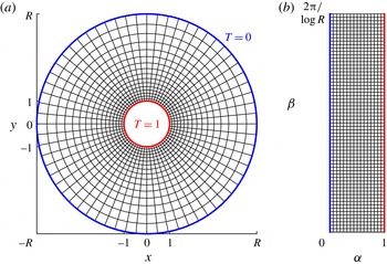
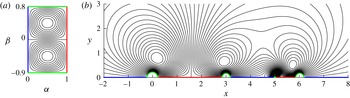
(a) Annular domain between the inner (hot) boundary at radius 1 and the outer (cold) boundary at radius  $R$ . The curvilinear grid plots equicontours of the conformal coordinates $\unicode[STIX]{x1D6FC}=1-\log r/\log R$ and $\unicode[STIX]{x1D6FD}=-\unicode[STIX]{x1D703}/\log R$ where $r$ and $\unicode[STIX]{x1D703}$ are the radial and angular coordinates, respectively. (b) The flow domain in ( $\unicode[STIX]{x1D6FC},\unicode[STIX]{x1D6FD}$ ) coordinates.

We illustrate the general approach using a simple case in which the boundaries are concentric circles (see figure 1). The inner circle (radius 1) is the hot surface ( $T=1$ ) and the outer circle (radius $R>1$ ) is the cold surface ( $T=0$ ), and can be taken to represent a cold reservoir to which heat is transferred. We solve the problem for all $R>1$ , but the typical application would be the cooling of the exterior surface of an isolated heated body (Karniadakis Reference Karniadakis1988), in which case the reservoir is far away ( $R\gg 1$ ).

The flow $\boldsymbol{u}(x,y)=(u(x,y),v(x,y))$ satisfies incompressibility ( $\unicode[STIX]{x1D735}\boldsymbol{\cdot }\boldsymbol{u}=0$ ), so we write it in terms of the streamfunction $\unicode[STIX]{x1D713}(x,y)$ as $\boldsymbol{u}=-\unicode[STIX]{x1D735}^{\bot }\unicode[STIX]{x1D713}=(\unicode[STIX]{x2202}_{y}\unicode[STIX]{x1D713},-\unicode[STIX]{x2202}_{x}\unicode[STIX]{x1D713})$ . For a given flow field, the temperature field is obtained by solving the advection–diffusion equation

with thermal diffusivity $\unicode[STIX]{x1D705}$ . The flow field is constrained to have fixed kinetic energy  $KE$ ,

where $\unicode[STIX]{x1D70C}$ is the fluid density and $W$ is the domain width in the out-of-plane ( $z$ ) direction, along which all quantities are assumed to be invariant. The flow field is not explicitly constrained to satisfy the Navier–Stokes equations. However, any (sufficiently smooth) incompressible flow satisfies the incompressible Navier–Stokes equations with a suitable volume forcing term $\boldsymbol{f}$ ,

Given $\boldsymbol{u}$ , (2.3) determines $\boldsymbol{f}$ and $p$ . The flow can be considered to be driven by $\boldsymbol{f}$ .

We maximize the (steady) rate of heat flux out of the hot boundary,

Here, $k$ is the thermal conductivity of the fluid, $n$ is the coordinate normal to the boundary, increasing into the fluid domain, and $s$ is the arclength coordinate along the boundary, here just the negative of the angular coordinate along the boundary, increasing from 0 to $2\unicode[STIX]{x03C0}$ moving along the circle in the clockwise direction.

Non-dimensionalizing lengths by a typical length scale $L$ (in the present case, the radius of the inner cylinder) and time by a diffusion time scale $L^{2}/\unicode[STIX]{x1D705}$ , and writing $\boldsymbol{u}$ in terms of $\unicode[STIX]{x1D713}$ , (2.1) becomes

and (2.2) becomes

where the Péclet number $Pe=\sqrt{2KE/\unicode[STIX]{x1D70C}W\unicode[STIX]{x1D705}^{2}}$ measures the strength of advection relative to diffusion of heat, and is different from the definition of Hassanzadeh et al. (Reference Hassanzadeh, Chini and Doering2014) (which uses the average flow speed) because we will deal with unbounded fluid domains. We have already non-dimensionalized temperature by the temperature of the hot boundary (also the temperature difference between the boundaries). Having chosen scales for length, time and temperature, we need to choose a typical mass scale to non-dimensionalize (2.4). Since mass enters the thermal conductivity, for simplicity we instead chose the thermal conductivity scale to be that of the fluid, so that, in dimensionless form, (2.4) becomes

We maximize $Q$ over all steady 2D incompressible flow fields (given by $\unicode[STIX]{x1D713}$ ) of a given kinetic energy by taking the variation of the Lagrangian

Here, $m$ and $\unicode[STIX]{x1D706}$ are Lagrange multipliers enforcing (2.5) and (2.6) respectively. The area integrals are over the fluid domain, the annulus in figure 1(a). The optimal $\unicode[STIX]{x1D713}$ is found by setting to zero the variations of ${\mathcal{L}}$ with respect to $T$ , $\unicode[STIX]{x1D713}$ , $m$ and $\unicode[STIX]{x1D706}$ . Taking the variations and integrating by parts, we obtain the following equations and boundary conditions:

The boundary conditions in (2.10) make the boundary terms in $\unicode[STIX]{x1D6FF}{\mathcal{L}}/\unicode[STIX]{x1D6FF}T$ (not shown) equal to zero. The boundary conditions for (2.11) are due to the fact that the boundaries are solid walls with no flow penetration. There is slip along the walls, and the flow may be taken as an approximation of the flow that would occur with no-slip boundary conditions. No-slip boundary conditions arise naturally when we consider the problem with fixed enstrophy later in this work. The constant for $\unicode[STIX]{x1D713}$ may be taken to be zero on one boundary (the inner cylinder), to remove arbitrariness in $\unicode[STIX]{x1D713}$ . On other boundaries (here, the outer cylinder), the constant values of $\unicode[STIX]{x1D713}$ are unknowns set by the equation

on each such boundary. The integral in (2.13) is $\unicode[STIX]{x1D6FF}{\mathcal{L}}/\unicode[STIX]{x1D6FF}\unicode[STIX]{x1D713}$ on the boundaries (on each of which $\unicode[STIX]{x1D6FF}\unicode[STIX]{x1D713}$ is uniform), and is therefore zero where $\unicode[STIX]{x1D713}$ is not prescribed. Our approach is essentially the same as that of Hassanzadeh et al. (Reference Hassanzadeh, Chini and Doering2014) so far. To solve the problem in this annular geometry, and in a general class of geometries, it is convenient to change coordinates. Let $T_{0}$ denote the temperature with the given boundary conditions and no flow, determined purely by conduction, $\unicode[STIX]{x0394}T_{0}=0$ . Here, $T_{0}$ is a harmonic function, given by $1-\log r/\log R$ . It has a harmonic conjugate function $\unicode[STIX]{x1D6FD}=-\unicode[STIX]{x1D703}/\log R$ which is related to $T_{0}$ by the Cauchy–Riemann equations, $\unicode[STIX]{x2202}_{x}T_{0}=\unicode[STIX]{x2202}_{y}\unicode[STIX]{x1D6FD}$ , $\unicode[STIX]{x2202}_{y}T_{0}=-\unicode[STIX]{x2202}_{x}\unicode[STIX]{x1D6FD}$ . Because the flow domain is doubly connected, $\unicode[STIX]{x1D6FD}$ is multi-valued; for simply connected domains, a single-valued harmonic conjugate always exists (Brown, Churchill & Lapidus Reference Brown, Churchill and Lapidus1996). The term $\unicode[STIX]{x1D6FD}$ is unique up to an additive constant. Here, $(T_{0},\unicode[STIX]{x1D6FD})$ are conformal coordinates, and we will show that (2.9)–(2.12) are essentially unchanged in these coordinates. However, the flow domain transforms into a rectangle, and we will show that this maps the problem to the one solved by Hassanzadeh et al. (Reference Hassanzadeh, Chini and Doering2014). For notational convenience, we set $\unicode[STIX]{x1D6FC}(x,y)\equiv T_{0}(x,y)$ and use $\unicode[STIX]{x1D6FC}$ as the coordinate name. The metric that gives the density of $(\unicode[STIX]{x1D6FC},\unicode[STIX]{x1D6FD})$ equicontours in the $(x,y)$ plane is

Writing $\unicode[STIX]{x1D735}$ , $\unicode[STIX]{x1D735}^{\bot }$ and $\unicode[STIX]{x1D6E5}$ in $(\unicode[STIX]{x1D6FC},\unicode[STIX]{x1D6FD})$ coordinates using standard formulae for differential operators in orthogonal curvilinear coordinates (Acheson Reference Acheson1990), we have

Therefore, (2.9)–(2.11) are unchanged in $(\unicode[STIX]{x1D6FC},\unicode[STIX]{x1D6FD})$ coordinates, and so is (2.12) when the integral is written in $(\unicode[STIX]{x1D6FC},\unicode[STIX]{x1D6FD})$ coordinates,

The boundary conditions are also unchanged, except that they are given on the sides of a rectangle (figure 1 b). Thus, the problem is essentially the same as that solved by Hassanzadeh et al. (Reference Hassanzadeh, Chini and Doering2014), with $(\unicode[STIX]{x1D6FC},\unicode[STIX]{x1D6FD})$ here corresponding to $(1-z,x)$ there. Instead of maximizing (2.7), they maximized the convective heat flux integrated over the flow domain. In appendix A we show that the two are equal in curvilinear coordinates, so that in place of (2.7) we can use

where $\unicode[STIX]{x0394}\unicode[STIX]{x1D6FD}\equiv \unicode[STIX]{x1D6FD}_{max}-\unicode[STIX]{x1D6FD}_{min}$ is the extent of the domain in $\unicode[STIX]{x1D6FD}$ . Equation (2.17) allows one to compute the leading contributions to $Q$ in the small- $Pe$ limit from the solution to a single eigenvalue problem.

In the limit of small $Pe$ , the solutions can be written as asymptotic series in powers of $Pe$ . When $Pe=0$ , the solutions to (2.9)–(2.12) are

Asymptotic solutions to (2.9)–(2.12) for $0<Pe\ll 1$ are therefore posed as

Expanding (2.9)–(2.12) to $O(Pe)$ yields linearized equations for $T_{1}$ , $m_{1}$ and $\unicode[STIX]{x1D713}_{1}$ ,

Examining (2.22) and (2.23) and using $m_{0}=T_{0}$ , we find that $m_{1}=-T_{1}$ , so we can eliminate $m_{0}$ and $m_{1}$ and reduce (2.22)–(2.25) to

Using $\unicode[STIX]{x1D735}T_{0}=\hat{\boldsymbol{e}}_{\unicode[STIX]{x1D6FC}}/h$ , the system simplifies to

Because the boundary conditions are periodic in $\unicode[STIX]{x1D6FD}$ , the eigenfunctions may be found by taking a Fourier transform of (2.29)–(2.30) in $\unicode[STIX]{x1D6FD}$ (or $x$ in Hassanzadeh et al. (Reference Hassanzadeh, Chini and Doering2014)). We obtain

where $\unicode[STIX]{x0394}\unicode[STIX]{x1D6FD}=2\unicode[STIX]{x03C0}/\log R$ . We may add an arbitrary constant phase to $\unicode[STIX]{x1D6FD}$ which simply rotates the solutions without changing the total kinetic energy or the heat transferred. The flow corresponding to (2.32) is an array of convection rolls in $(\unicode[STIX]{x1D6FC},\unicode[STIX]{x1D6FD})$ space. Inserting (2.32)–(2.33) into (2.29)–(2.30), we obtain $A_{kn}$ , $B_{kn}$ and $\unicode[STIX]{x1D706}$ ,

The heat transferred by each mode (2.17) can be expanded in orders of $Pe$ . The zeroth-order term is $Q_{0}=\unicode[STIX]{x0394}\unicode[STIX]{x1D6FD}$ . The first-order term $Q_{1}$ vanishes for each mode (2.32)–(2.33), so the leading-order term to be maximized is

This term is maximum when $k=1$ and if $\unicode[STIX]{x0394}\unicode[STIX]{x1D6FD}/2$ is an integer, when $n=\unicode[STIX]{x0394}\unicode[STIX]{x1D6FD}/2$ . In this case, $Q_{2,max}=1/4\unicode[STIX]{x03C0}^{2}$ . If $\unicode[STIX]{x0394}\unicode[STIX]{x1D6FD}/2$ is not an integer but lies between the integers $l$ and $l+1$ , then the $Q_{2}$ -maximizing $n$ is $l$ if $\unicode[STIX]{x0394}\unicode[STIX]{x1D6FD}/2<\sqrt{l(l+1)}$ and $l+1$ otherwise. 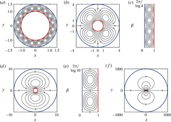The $Q_{2}$ -maximizing flow is a mode (2.32) consisting of approximately square convection rolls in $(\unicode[STIX]{x1D6FC},\unicode[STIX]{x1D6FD})$ space. In figure 2, we plot the streamlines at equal intervals of the streamfunction for $Q_{2}$ -maximizing flows when the outer boundary radius is $R=1.5$ , 4, 10 and 1000.

Figure 2.

Streamlines for optimal convection cooling flows in annular domains in the small- $Pe$ limit (small kinetic energy). The outer (cold) boundary has different radii $R=1.5$ (a), 4 (b), 10 (d) and 1000 (f). The inner (hot) boundary has radius 1. Panels (c) and (e) show the flows in (b) and (d) in $(\unicode[STIX]{x1D6FC},\unicode[STIX]{x1D6FD})$ coordinates. The streamlines are plotted at nine equally spaced values between the extrema of the streamfunction. In (b,d–f), the arrows indicate one of the two possible flow directions for these optima; the reversed flow gives the same heat transfer.

When $R$ is close to 1 (a), we have a thin gap between the hot and cold surfaces, and the flows tend to the square convection rolls in a straight channel found by Hassanzadeh et al. (Reference Hassanzadeh, Chini and Doering2014). Since $h$ in (2.14) is $r\log R$ , which varies little in the thin gap, there is relatively little distortion when the vortices are mapped from the $(\unicode[STIX]{x1D6FC},\unicode[STIX]{x1D6FD})$ plane to the $(x,y)$ plane. The case $R\gg 1$ corresponds to the application of the convection cooling of the exterior of a circular body. In this limit (e.g. (f)), the optimal flow is

which consists of a pair of oppositely signed vortices forming a dipole near the body. The amount of vortex distortion is given by $h=r\log R$ , so the vortices are strongly stretched moving outward from the body. The centres of the vortices are located at $r=\sqrt{R}$ , the local extrema of $\unicode[STIX]{x1D713}_{max}$ . Differentiating (2.38) with respect to $r$ , we find that the azimuthal flow speed $u_{\unicode[STIX]{x1D703}}$ is proportional to $\log ^{-1/2}R/r$ in the neighbourhood of the body ( $1\leqslant r\ll R$ ). The factor of $\log ^{-1/2}R$ allows the total kinetic energy to remain constant as $R\rightarrow \infty$ . When $\unicode[STIX]{x0394}\unicode[STIX]{x1D6FD}/2=\unicode[STIX]{x03C0}/\log R$ is an integer, $Q_{2,max}=1/4\unicode[STIX]{x03C0}^{2}$ . For large $R$ , $Q_{2,max}$ is attained with $n=k=1$ . Consequently, with a fixed total kinetic energy, the optimal heat transferred by convection ( $Pe^{2}Q_{2,max}\sim Pe^{2}\log ^{-2}R$ ) decays slowly as the outer radius increases. Physically, it seems reasonable that the optimal heat transferred with fixed kinetic energy should decrease as the hot and cold surfaces become more distant. We also note that the annulus problem is singular in the limit $R\rightarrow \infty$ , as the steady conduction temperature ( $\unicode[STIX]{x1D6FC}$ ) is not well defined for $R=\infty$ .

We have discussed optimal convection cooling using the specific example of an annular geometry, but similar results can be obtained for a wide range of geometries. The first step is to compute $(\unicode[STIX]{x1D6FC},\unicode[STIX]{x1D6FD})$ for a given geometry. In the next two sections, we discuss the solutions for two geometries that are relevant to applications. We find that a slight modification is needed in cases where the hot and cold surfaces meet.

3 Hot plate embedded in a cold surface

The next geometry we consider is a hot plate embedded in a cold surface (see figure 3). The hot plate gives a simple model of a flat heated surface such as a computer processor. An important difference from the previous case is that the cold and hot surfaces are now connected (or nearly so, as we will discuss). We non-dimensionalize by the length of the plate.

Figure 3.

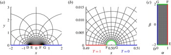
(a) A portion of the flow domain – the upper half-plane – near the hot boundary. The hot boundary extends nearly to the limits of the interval ( $|x|\leqslant 1/2,y=0$ ). The cold boundaries are approximately ( $|x|>1/2,y=0$ ). They are joined by small insulating boundaries which are approximately semi-circular. The curvilinear grid plots equicontours of the conformal coordinates $\unicode[STIX]{x1D6FC}=(\arg (z-1/2)-\arg (z+1/2))/\unicode[STIX]{x03C0}$ and $\unicode[STIX]{x1D6FD}=-\log |(z-1/2)/(z+1/2)|/\unicode[STIX]{x03C0}$ . (b) Close-up near $z=1/2$ . The approximate semi-circle closest to $1/2$ (light grey or green) is the contour $\unicode[STIX]{x1D6FD}=2$ . This is one of the insulating boundaries of the truncated domain, with the other located near $z=-1/2$ . (c) The flow domain in ( $\unicode[STIX]{x1D6FC},\unicode[STIX]{x1D6FD}$ ) space. The letters D–G show corresponding points in (a), (b) and (c).

The plate (where $T=1$ ) occupies $-1/2\leqslant x\leqslant 1/2$ on the real axis, and the cold surface (where $T=0$ ) is $|x|>1/2$ . The fluid lies in the upper half-plane, $y>0$ . In terms of the complex coordinate $z=x+\text{i}y$ , the pure conduction solution (with $Pe=0$ ) is

Following the same procedure as before,

These are also known as bipolar coordinates, with foci at $x=\pm 1/2$ . In these coordinates, the flow domain is $0<\unicode[STIX]{x1D6FC}<1$ , $-\infty <\unicode[STIX]{x1D6FD}<\infty$ . The problem is no longer periodic in $\unicode[STIX]{x1D6FD}$ , and new boundary conditions are required at $\unicode[STIX]{x1D6FD}=\pm \infty$ . To proceed, we first truncate the domain to $0<\unicode[STIX]{x1D6FC}<1$ , $\unicode[STIX]{x1D6FD}_{min}<\unicode[STIX]{x1D6FD}<\unicode[STIX]{x1D6FD}_{max}$ , introducing new boundaries at finite values $\unicode[STIX]{x1D6FD}_{min}<0$ and $\unicode[STIX]{x1D6FD}_{max}>0$ . By (3.2a,b ), the distances of the boundaries from $z=\pm 1/2$ decay exponentially fast ( ${\sim}\text{e}^{-|\unicode[STIX]{x1D6FD}_{min}|\unicode[STIX]{x03C0}}$ , $\text{e}^{-|\unicode[STIX]{x1D6FD}_{max}|\unicode[STIX]{x03C0}}$ ) as $\unicode[STIX]{x1D6FD}_{min}$ and $\unicode[STIX]{x1D6FD}_{max}$ grow in magnitude. Therefore, with moderate values of $\unicode[STIX]{x1D6FD}_{min}$ and $\unicode[STIX]{x1D6FD}_{max}$ , we obtain a good approximation to the original non-truncated domain in the $(x,y)$ plane.

We find that the leading-order solution for $T$ is still $T_{0}$ if we make the new boundaries insulating, so $0=\unicode[STIX]{x2202}_{n}T=\unicode[STIX]{x2202}_{\unicode[STIX]{x1D6FD}}T/h$ . The term $T_{0}$ satisfies this boundary condition because $\unicode[STIX]{x2202}_{\unicode[STIX]{x1D6FD}}T_{0}=\unicode[STIX]{x2202}_{\unicode[STIX]{x1D6FD}}\unicode[STIX]{x1D6FC}=0$ ( $\unicode[STIX]{x1D6FC}$ and $\unicode[STIX]{x1D6FD}$ are orthogonal coordinates). Recomputing the variation of ${\mathcal{L}}$ with these Neumann (instead of periodic) conditions at the $\unicode[STIX]{x1D6FD}$ boundaries, we find that $m$ has the same boundary conditions as $T$ , and thus, as before, $m_{0}=T_{0}$ , $m_{1}=-T_{1}$ . We assume that the insulating boundaries are solid walls that the flow does not penetrate. Because they are connected to the hot and cold boundaries, this requires $\unicode[STIX]{x1D713}=0$ on all four sides of the rectangular domain in $(\unicode[STIX]{x1D6FC},\unicode[STIX]{x1D6FD})$ space. Thus, we obtain the same eigenvalue problem as (2.29)–(2.31) but with $\unicode[STIX]{x2202}_{n}T_{1}=\unicode[STIX]{x1D713}_{1}=0$ on the insulating sides of the rectangle. The eigenfunctions are slightly modified from (2.32)–(2.33),

with

Because the Neumann boundaries are solid insulating walls, (2.17) still holds, and $Q_{2}$ , the leading contribution to the heat transferred by a given mode, is

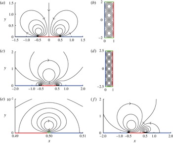
This term is maximized when $k=1$ and $n$ is one of the two integers closest to $\unicode[STIX]{x0394}\unicode[STIX]{x1D6FD}$ , which again results in convection rolls that are square (or nearly so, if $\unicode[STIX]{x0394}\unicode[STIX]{x1D6FD}$ is not an integer) in $(\unicode[STIX]{x1D6FC},\unicode[STIX]{x1D6FD})$ space. In figure 4, we show examples of optimal flows when $\unicode[STIX]{x0394}\unicode[STIX]{x1D6FD}$ is even (a) and odd (c and f).

Figure 4.

(a) Optimal heat transferring flow with $\unicode[STIX]{x1D6FD}_{min}=-2$ and $\unicode[STIX]{x1D6FD}_{max}=2$ . The flow has four vortices: one pair of large vortices of the order of the plate length and one pair of small vortices of the order of the insulating boundary length. (b) The flow from (a) in $(\unicode[STIX]{x1D6FC},\unicode[STIX]{x1D6FD})$ coordinates. (c) Optimal heat transferring flow with $\unicode[STIX]{x1D6FD}_{min}=-2.5$ and $\unicode[STIX]{x1D6FD}_{max}=2.5$ . The flow has five vortices: one large vortex centred over the plate and two pairs symmetric about the $y$ axis. (d) The flow from (c) in $(\unicode[STIX]{x1D6FC},\unicode[STIX]{x1D6FD})$ coordinates. (e) Close-up of the flow in (c) near $z=1/2$ , showing one of the smaller vortices, near the insulated boundary (light grey or green). (f) Example of an asymmetric flow with $\unicode[STIX]{x1D6FD}_{min}=-2.75$ , $\unicode[STIX]{x1D6FD}_{max}=2.25$ . Five vortices are present, and the two nearest the insulated boundaries are too small to be visible. In (a,c,e,f), the arrows indicate one of the two possible flow directions for these optima; the reversed flow gives the same heat transfer.

We have a chain of vortices, which are $O(1)$ in size above the hot plate and shrink exponentially in size as they approach the insulated boundaries at the hot–cold interface. In (a), $\unicode[STIX]{x1D6FD}_{min}=-2$ and $\unicode[STIX]{x1D6FD}_{max}=2$ , and there are four vortices, one large pair and one small pair. The smallest vortices are proportional in size to the insulated boundaries. Panel (b) shows the same flow in the $(\unicode[STIX]{x1D6FC},\unicode[STIX]{x1D6FD})$ plane. Panel (c) shows the optimal flow with $\unicode[STIX]{x1D6FD}_{min}=-2.5$ and $\unicode[STIX]{x1D6FD}_{max}=2.5$ , so there are five vortices (the smallest pair is not visible). Panel (d) shows this flow in the $(\unicode[STIX]{x1D6FC},\unicode[STIX]{x1D6FD})$ plane. Panel (e) shows the flow near one of the small vortices in (c) at the insulated boundary near $z=1/2$ . Panel (f) shows an asymmetric case, $\unicode[STIX]{x1D6FD}_{min}=-2.75$ and $\unicode[STIX]{x1D6FD}_{max}=2.25$ . Again there are five vortices, but now they are asymmetric with respect to the plate centre. The size of each vortex is proportional to its distance from the insulated boundary, and the typical flow speed within each vortex is inversely proportional to its size. Therefore, as the vortices become smaller, the flow speed increases, such that the total kinetic energy of each vortex (proportional to its area times the typical flow speed squared) is constant.

Once again, $Q_{2,max}=1/4\unicode[STIX]{x03C0}^{2}$ (when $\unicode[STIX]{x0394}\unicode[STIX]{x1D6FD}$ is an integer), so the optimal heat transferred by convection is essentially the same when we vary the positions of the insulating boundaries. The optimal flow varies considerably with the positions of the insulating boundaries, however, because they set the positions of the vortices. It is somewhat surprising that the optimal heat transferred by convection does not increase as the hot and cold surfaces are brought together (for the annulus, we found a slow decrease in the heat transferred by convection when the surfaces become more distant). However, the heat transferred by conduction ( $\unicode[STIX]{x0394}\unicode[STIX]{x1D6FD}$ ) diverges logarithmically as the distance between the hot and cold surfaces tends to zero.

4 Channel with hot interior and cold exterior

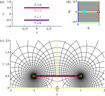
A classic configuration for heat transfer is the flow through a heated channel (Eagle & Ferguson Reference Eagle and Ferguson1930; Dipprey & Sabersky Reference Dipprey and Sabersky1963; Bird et al. Reference Bird, Stewart and Lightfoot2007; Bejan Reference Bejan2013; Lienhard Reference Lienhard2013). Recent works have studied the dynamics of flapping flags and vortex streets in channels (Alben Reference Alben2015; Wang & Alben Reference Wang and Alben2015) with the goal of improving heat transfer efficiency by using vortices to mix the temperature field (Gerty Reference Gerty2008; Shoele & Mittal Reference Shoele and Mittal2014; Jha et al. Reference Jha, Hidalgo and Glezer2015). Here, we consider a heated channel in an unbounded fluid (figure 5 a).

Figure 5.

(a) Heated channel in an unbounded flow domain. The inside surfaces of the channel walls have temperature $T=1$ and the outside surfaces have $T=0$ . (b) The flow domain in $\unicode[STIX]{x1D6FC},\unicode[STIX]{x1D6FD}$ space for the case $L=2,\unicode[STIX]{x1D6FD}_{min}=-0.5$ and $\unicode[STIX]{x1D6FD}_{max}=0.5$ . The light blue (light grey) dot marks the point at infinity and the black triangle marks the origin in $(x,y)$ space. The green boundaries are insulated surfaces, and the red and blue boundaries are the hot and cold surfaces of the upper channel wall. (c) The upper half of the flow domain in $(x,y)$ space. The red, blue, green and yellow lines and triangle correspond to those in (b). The curvilinear grid plots equicontours of $\unicode[STIX]{x1D6FC}$ and $\unicode[STIX]{x1D6FD}$ .

The inside surfaces of the channel walls are fixed at temperature $T=1$ and the outside surfaces are fixed at $T=0$ . If we assume that the channel flow is a perturbation of unidirectional flow, we could possibly truncate the fluid domain to the interior of the channel, and use inflow and outflow boundary conditions for the fluid and temperature (Shoele & Mittal Reference Shoele and Mittal2014; Wang & Alben Reference Wang and Alben2015). However, we wish to make minimal assumptions about the flow and therefore we represent the flow both inside and outside the channel. Energy is needed to drive the flow through the entire fluid domain, so it makes sense to include the outside flow in the optimization calculation.

The analytic function $\unicode[STIX]{x1D6FC}+\text{i}\unicode[STIX]{x1D6FD}$ can be found numerically by using complex analysis and boundary integral methods. Because $T$ (and therefore $\unicode[STIX]{x1D6FC}$ ) has a jump across the channel walls, we can write $\unicode[STIX]{x1D6FC}+\text{i}\unicode[STIX]{x1D6FD}$ as a Cauchy-type integral (see appendix B and Estrada & Kanwal (Reference Estrada and Kanwal2012) for background),

where $C$ is a complex contour parametrized by arclength as $\unicode[STIX]{x1D701}(s)$ , representing the union of the two channel walls, $s\pm \text{i}/2,-L/2<s<L/2$ . The real constant $C_{1}$ will be chosen shortly. The function $\unicode[STIX]{x1D6FE}+\text{i}\unicode[STIX]{x1D702}$ corresponds to the jump in $\unicode[STIX]{x1D6FC}+\text{i}\unicode[STIX]{x1D6FD}$ along the contour. From the boundary conditions on $\unicode[STIX]{x1D6FC}$ (those of $T$ ), we have $\unicode[STIX]{x1D6FE}=\pm 1$ on $\unicode[STIX]{x1D701}(s)=s\pm \text{i}/2$ . It remains to find $\unicode[STIX]{x1D702}$ , which we now write as $\unicode[STIX]{x1D702}(s)$ , a function of  $s$ . We note that (4.1) provides the average value of $\unicode[STIX]{x1D6FC}+\text{i}\unicode[STIX]{x1D6FD}$ on the contour when $z$ is a point on the contour and the integral is changed from an ordinary integral to a principal value integral (one of the Plemelj formulae; see appendix B and Estrada & Kanwal (Reference Estrada and Kanwal2012)). We solve for $\unicode[STIX]{x1D702}(s)$ by the condition that the average value of $\unicode[STIX]{x1D6FC}$ on the contour equals $1/2$ ,

We have written the contributions from the two channel walls in (4.1) separately and used symmetry considerations to deduce that $\unicode[STIX]{x1D702}$ on the lower wall equals that on the upper wall. We use the Chebyshev collocation method (Golberg Reference Golberg1990) to solve (4.2) with $s$ at points on a Chebyshev–Lobatto grid and $s^{\prime }$ on a Chebyshev–Gauss grid. We need two additional constraints to uniquely specify $\unicode[STIX]{x1D702}$ and $C_{1}$ in (4.2) (Golberg Reference Golberg1990). These can be given as

These conditions remove the inverse-square-root singularities at the contour edges which occur generically in solutions to Cauchy integral equations such as $\unicode[STIX]{x1D702}$ in (4.1) (Golberg Reference Golberg1990). Having solved for $\unicode[STIX]{x1D702}$ and $C_{1}$ and knowing $\unicode[STIX]{x1D6FE}$ , we evaluate $\unicode[STIX]{x1D6FC}$ and $\unicode[STIX]{x1D6FD}$ using (4.1). As with the single heated plate, we find that $\unicode[STIX]{x1D6FD}\rightarrow \pm \infty$ at the plate edges where the hot and cold boundaries meet. Therefore, as before, we cut off the domain with small insulated boundaries at $\unicode[STIX]{x1D6FD}=\unicode[STIX]{x1D6FD}_{min}$ and $\unicode[STIX]{x1D6FD}_{max}$ . In figure 5(b,c), we show $(\unicode[STIX]{x1D6FC},\unicode[STIX]{x1D6FD})$ equicontours and their location in the $(x,y)$ plane respectively for the case $L=2$ . Here, we use $\unicode[STIX]{x1D6FD}_{min}=-0.5,\unicode[STIX]{x1D6FD}_{max}=0.5$ . These values are relatively small in magnitude so that the insulated boundaries are large enough to be clearly visible. As with the single heated plate example, the insulated boundaries approach the plate edges exponentially with increasing magnitude of these values.

In (c), we show only the upper half-plane in $(x,y)$ . In the lower half-plane, the values of $\unicode[STIX]{x1D6FC}$ and $\unicode[STIX]{x1D6FD}$ can be smoothly continued from the upper half-plane, by reflecting the values in the origin. Thus, the flow is also smoothly continued in the lower half-plane by reflecting $\unicode[STIX]{x1D713}$ in the origin.

Figure 6.

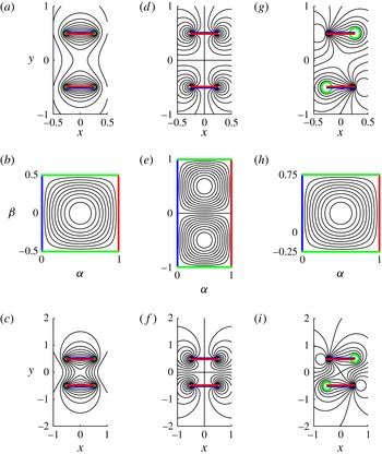
Streamlines of optimal heat transferring flows for short channels. The channel lengths are $L=0.5$ in (a,d,g) and 1 in (c,f,i). Panels (b,e,h) show the flows from (a,d,g) and (c,f,i) in $(\unicode[STIX]{x1D6FC},\unicode[STIX]{x1D6FD})$ coordinates, where they are the same. The positions of the insulated boundaries (green) vary: $\unicode[STIX]{x1D6FD}_{min}=-0.5$ and $\unicode[STIX]{x1D6FD}_{max}=0.5$ (a–c); $\unicode[STIX]{x1D6FD}_{min}=-1$ and $\unicode[STIX]{x1D6FD}_{max}=1$ (d–f), too close to the plate edges to be visible; $\unicode[STIX]{x1D6FD}_{min}=-0.25$ and $\unicode[STIX]{x1D6FD}_{max}=0.75$ (g–i).

In figure 6, we show optimal flows for ‘short’ channels, with lengths less than or equal to the channel height. Panels (a,d,g) show optimal flows when the channel length is half of the height. The only difference between (a), (d) and (g) is the location of the insulating boundaries. As we have seen with the single plate, this makes a big difference in the optimal flow. In (a), the flow consists of rolls that move around the plates. There is a strong net flow through the channel, which is fast near the channel walls and slow in the middle of the channel. The corresponding flow in the $(\unicode[STIX]{x1D6FC},\unicode[STIX]{x1D6FD})$ plane is shown in (b). It is a single vortex which is mapped twice onto the $(x,y)$ plane in (a) by reflection in the origin, as mentioned previously. In (d), we move the insulating boundaries closer to the plate edges, and obtain two pairs of vortices moving around the edges of the channel. The flow is fastest near the plate edges, where the hot and cold surfaces are closest. Panel (e) shows the corresponding flow in the $(\unicode[STIX]{x1D6FC},\unicode[STIX]{x1D6FD})$ plane. Panel (g) shows an example in which the insulating boundaries are asymmetric in $\unicode[STIX]{x1D6FD}$ , with the $(\unicode[STIX]{x1D6FC},\unicode[STIX]{x1D6FD})$ representation shown in (h).

Panels (c,f,i) show optimal flows when the channel length equals its height. The corresponding flows in the $(\unicode[STIX]{x1D6FC},\unicode[STIX]{x1D6FD})$ plane are again those in (b,e,h). In (c), the flow has a stronger circulatory component, which moves across the channel openings, from top to bottom and vice versa, around the outside of the entire channel, compared with that in (a). In (f) and (i), the flow is also stronger near the centres of the channel openings than in the corresponding flows of (d) and (g).

Figure 7.

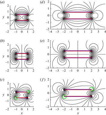
Streamlines of optimal heat transferring flows for longer channels (lengths $L=2$ (a–c) and 4 (d–f) in units of channel width). For the length-2 channels (a–c), the insulated boundaries (green) are located at (a) $\unicode[STIX]{x1D6FD}_{min}=-0.5$ and $\unicode[STIX]{x1D6FD}_{max}=0.5$ , (b) $\unicode[STIX]{x1D6FD}_{min}=-1$ and $\unicode[STIX]{x1D6FD}_{max}=1$ (too close to the plate edges to be visible), and (c) $\unicode[STIX]{x1D6FD}_{min}=-0.25$ and $\unicode[STIX]{x1D6FD}_{max}=0.75$ . For the length-4 channels (d–f), the insulated boundaries (green) are located at (d) $\unicode[STIX]{x1D6FD}_{min}=-0.5$ and $\unicode[STIX]{x1D6FD}_{max}=0.5$ , (e) $\unicode[STIX]{x1D6FD}_{min}=-1$ and $\unicode[STIX]{x1D6FD}_{max}=1$ (too close to the plate edges to be visible), and (f) $\unicode[STIX]{x1D6FD}_{min}=-0.25$ and $\unicode[STIX]{x1D6FD}_{max}=0.75$ .

In figure 7, we show optimal flows when the channel length is increased to two (a–c) and four (d–f) times the channel height. Now, the flows are strongly confined to the channel openings. There is very little flow in the centre of the channel. The reason is that the temperature due to pure conduction ( $T_{0}=\unicode[STIX]{x1D6FC}$ ) is nearly uniform in the centre of the channel. There is little to be gained by using energy to transport fluid through this region of nearly uniform temperature. Since $\unicode[STIX]{x1D6FC}$ changes little in this region, $h=\Vert \unicode[STIX]{x2202}\boldsymbol{X}/\unicode[STIX]{x2202}\unicode[STIX]{x1D6FC}\Vert =\Vert \unicode[STIX]{x2202}\boldsymbol{X}/\unicode[STIX]{x2202}\unicode[STIX]{x1D6FD}\Vert \gg 1$ and the flow speed $\Vert \boldsymbol{u}\Vert =\Vert -\unicode[STIX]{x1D735}_{x,y}^{\bot }\unicode[STIX]{x1D713}\Vert =\Vert -\unicode[STIX]{x1D735}_{\unicode[STIX]{x1D6FC},\unicode[STIX]{x1D6FD}}^{\bot }\unicode[STIX]{x1D713}/h\Vert \sim 1/h\ll 1.$ The lack of flow through the channel is a significant difference from typical channel convection cooling flows (Bird et al. Reference Bird, Stewart and Lightfoot2007). This can be attributed to our objective of maximizing the total heat flux out of the hot walls. In these solutions, most of the flux is close to the channel openings, near the cold exterior.

5 Large-amplitude flows

We now consider the case where $Pe$ is not small by returning to (2.9)–(2.12), which holds for all $Pe\geqslant 0$ . We have noted that this is the same as the constant-kinetic-energy problem considered by Hassanzadeh et al. (Reference Hassanzadeh, Chini and Doering2014) under the transformation $(\unicode[STIX]{x1D6FC},\unicode[STIX]{x1D6FD})\rightarrow (1-z,x)$ . They computed numerically the solutions from $Pe$ small to large and derived a boundary layer solution for the optimal flow in the limit of large $Pe$ . Their derivation works for both the periodic and Neumann boundary conditions (in $\unicode[STIX]{x1D6FD}$ ) that we used here. We simply translate the complete asymptotic solution for $\unicode[STIX]{x1D713}$ that they found into an $(\unicode[STIX]{x1D6FC},\unicode[STIX]{x1D6FD})$ rectangle with $\unicode[STIX]{x1D6FD}$ -width $\unicode[STIX]{x0394}\unicode[STIX]{x1D6FD}$ ,

In the limit of large $Pe$ , equal-aspect-ratio convection rolls are no longer optimal. Instead, the convection rolls become very narrow in the $\unicode[STIX]{x1D6FD}$ direction, with narrow boundary layers of fast-moving fluid along the hot and cold walls. The size of the boundary layers and the $\unicode[STIX]{x1D6FD}$ -width of the rolls are set by the parameters $\unicode[STIX]{x1D6E4}$ and $\unicode[STIX]{x1D707}_{H},(=,2\unicode[STIX]{x1D706})$ in (5.1). For $Pe\gg 1$ , Hassanzadeh et al. (Reference Hassanzadeh, Chini and Doering2014) found that for the optimal rolls,

where we have added the $\unicode[STIX]{x0394}\unicode[STIX]{x1D6FD}$ term due to our different definition of $Pe$ . This solution is valid for our problems with Neumann conditions at the $\unicode[STIX]{x1D6FD}$ boundaries when $\unicode[STIX]{x0394}\unicode[STIX]{x1D6FD}/\unicode[STIX]{x1D6E4}$ is an integer, $N$ in (5.1). For periodic boundary conditions, $N$ must be even.

Figure 8.

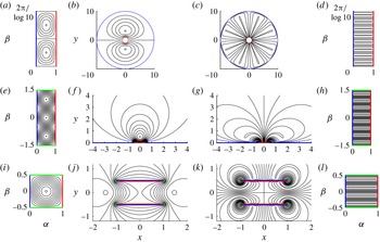
A comparison of optimal flows with small and large kinetic energy ( $Pe$ ) across the three geometries considered in this work. (a–d) Optimal flows in an annulus with outer radius $R=10$ . (a) Small- $Pe$ optimal flow in $(\unicode[STIX]{x1D6FC},\unicode[STIX]{x1D6FD})$ . (b) Small- $Pe$ optimal flow in $(x,y)$ . (c) Large- $Pe$ ( $Pe\approx$ 210) optimal flow in $(x,y)$ . (d) Large- $Pe$ ( $Pe\approx$ 210) optimal flow in $(\unicode[STIX]{x1D6FC},\unicode[STIX]{x1D6FD})$ . (e–h) Optimal flows over a hot plate embedded in a cold surface. (e) Small- $Pe$ optimal flow in $(\unicode[STIX]{x1D6FC},\unicode[STIX]{x1D6FD})$ . (f) Small- $Pe$ optimal flow in $(x,y)$ . (g) Large- $Pe$ ( $Pe\approx$ 182) optimal flow in $(x,y)$ . (h) Large- $Pe$ ( $Pe\approx$ 182) optimal flow in $(\unicode[STIX]{x1D6FC},\unicode[STIX]{x1D6FD})$ . (i–l) Optimal flows around a channel with hot interior and cold exterior. (i) Small- $Pe$ optimal flow in $(\unicode[STIX]{x1D6FC},\unicode[STIX]{x1D6FD})$ . (j) Small- $Pe$ optimal flow in $(x,y)$ . (k) Large- $Pe$ ( $Pe\approx$ 237) optimal flow in $(x,y)$ . (l) Large- $Pe$ ( $Pe\approx$ 237) optimal flow in $(\unicode[STIX]{x1D6FC},\unicode[STIX]{x1D6FD})$ .

In figure 8, we plot a few examples of optimal flows at moderately large $Pe$ for the geometries we have considered, together with the corresponding small- $Pe$ optima. In (a–d), we show flows past a cylinder with outer boundary at $R=10$ at small $Pe$ in $(\unicode[STIX]{x1D6FC},\unicode[STIX]{x1D6FD})$ (a) and $(x,y)$ (b), the same flows as in figure 2(d,e) respectively. The large- $Pe$ optimum is shown in (c) and (d) of figure 8. Here, $Pe\approx 210$ so that $N=8$ . The streamlines are approximately rectangles in $(\unicode[STIX]{x1D6FC},\unicode[STIX]{x1D6FD})$ (d), which map onto approximate wedges in $(x,y)$ (c). In (e–h), we show optimal flows over a hot plate at small $Pe$ ((e,f), similar to those in figure 4) and $Pe\approx 182$ (g,h). A given rectangular streamline in $(\unicode[STIX]{x1D6FC},\unicode[STIX]{x1D6FD})$ (h) maps onto a streamline that approximately follows one larger circle and one smaller circle (in the opposite direction) in the bipolar coordinate system (figure 3 a) connected by segments along the hot and cold plates. In (i–l), optimal flows in a channel of length 2 are shown at small $Pe$ (i,j) and $Pe\approx 237$ (k,l), giving $N=4$ . In this case, a rectangular streamline in $(\unicode[STIX]{x1D6FC},\unicode[STIX]{x1D6FD})$ maps onto a streamline that follows two arcs that are roughly circles centred at the channel edges. The arcs are again connected by segments along the hot and cold plates.

6 More general geometries

We have studied three examples which are representative of a more general class of problems which can be solved with the same method. The main step is to solve for $(\unicode[STIX]{x1D6FC}(x,y),\unicode[STIX]{x1D6FD}(x,y))$ . The first case, flow through an annulus, can be extended to any doubly connected region that lies between one simple closed curve on which the temperature is 1 and another on which the temperature is 0. The flow region may include the point at infinity. All such regions correspond to a rectangle in $(\unicode[STIX]{x1D6FC},\unicode[STIX]{x1D6FD})$ space on which the boundary conditions for $\unicode[STIX]{x1D713}$ and $T$ are Dirichlet on the $\unicode[STIX]{x1D6FC}=0$ , $\unicode[STIX]{x1D6FC}=1$ sides and periodic on the $\unicode[STIX]{x1D6FD}=\unicode[STIX]{x1D6FD}_{min}$ , $\unicode[STIX]{x1D6FD}=\unicode[STIX]{x1D6FD}_{max}$ sides.

The second case, flow over a heated plate, can be generalized to the flow within any region bounded by a simple closed curve that is partitioned into four arcs. On the four arcs, the boundary conditions are $T=0$ , $\unicode[STIX]{x2202}_{n}T=0$ , $T=1$ and $\unicode[STIX]{x2202}_{n}T=0$ , moving continuously around the curve. On the entire curve, $\unicode[STIX]{x1D713}=0$ . The curve may include the point at infinity (as for the heated plate), and in general we may use any simple closed curve on the Riemann sphere. On the arcs where $\unicode[STIX]{x2202}_{n}T=0$ , we have $0=\unicode[STIX]{x2202}_{n}T_{0}=\unicode[STIX]{x2202}_{n}\unicode[STIX]{x1D6FC}=-\unicode[STIX]{x2202}_{s}\unicode[STIX]{x1D6FD}$ , so $\unicode[STIX]{x1D6FD}$ is constant. All such cases correspond to a rectangle in $(\unicode[STIX]{x1D6FC},\unicode[STIX]{x1D6FD})$ space on which the boundary conditions are Dirichlet for $\unicode[STIX]{x1D713}$ , and Dirichlet and Neumann for $T$ on the $\unicode[STIX]{x1D6FC}$ and $\unicode[STIX]{x1D6FD}$ sides respectively. The green arcs in figures 3–7 were chosen because they followed lines of constant $\unicode[STIX]{x1D6FD}$ for functions that could be written in closed form or computed relatively easily, but the shapes of the insulated boundaries can be arbitrary in general.

The third case, flow through a heated channel, is an example where the flow lies in the region between two simple closed curves, each of which is partitioned into four arcs as above. Here, by symmetry, the same rectangle in $(\unicode[STIX]{x1D6FC},\unicode[STIX]{x1D6FD})$ was used to cover the $(x,y)$ space twice. This case can be generalized to non-symmetrical configurations of $n$ closed curves, and the curves may contain multiple arcs on which $T=0$ and $T=1$ .

Figure 9.

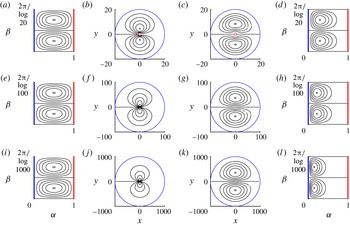
Optimal small-kinetic-energy flow (small $Pe$ ) over a surface with two hot plates (red) separated by cold plates (blue) and insulated boundaries (green), in $(\unicode[STIX]{x1D6FC},\unicode[STIX]{x1D6FD})$ (a) and $(x,y)$ (b). The flow is described by (3.3) with $\unicode[STIX]{x1D6FD}_{min}=-0.9$ , $\unicode[STIX]{x1D6FD}_{max}=0.8$ , and ( $\unicode[STIX]{x1D6FC},\unicode[STIX]{x1D6FD}$ ) given by (6.1a,b ).

Figure 9 shows an example where the flow domain is the upper half-plane, bounded by two hot and three cold segments along the $x$ axis. On the Riemann sphere, this is one closed curve on which the temperature is 1 on two arcs and 0 on two arcs. Here,

The rectangle with sides $\unicode[STIX]{x1D6FC}=0$ , $\unicode[STIX]{x1D6FC}=1$ , $\unicode[STIX]{x1D6FD}=-0.9$ , $\unicode[STIX]{x1D6FD}=0.8$ maps twice onto the flow region. Moving around the rectangle counterclockwise twice in (a) corresponds to moving along the boundary on the $x$ axis and green arcs in (b) from $x=-\infty$ to $+\infty$ . In the small- $Pe$ limit, the streamfunction is (3.3) with $n=2$ .

For general curvilinear domains, boundary integral methods like those in § 4 are applicable. For simplicity, in this work, we have used relatively simple geometries for the hot and cold surfaces, consisting of straight lines or circles. In more general versions of these cases, analytical methods can be used. When the fluid domain is a polygon, $\unicode[STIX]{x1D6FC}$ and $\unicode[STIX]{x1D6FD}$ can be computed using Schwarz–Christoffel methods (Ablowitz & Fokas Reference Ablowitz and Fokas2003; Crowdy Reference Crowdy2007). When the fluid domain is the exterior of multiple plates (like the channel in § 4), $\unicode[STIX]{x1D6FC}$ and $\unicode[STIX]{x1D6FD}$ can be derived using the Schottky–Klein prime function, following the methods of Crowdy (Reference Crowdy2007, Reference Crowdy2012).

7 Fixed-enstrophy flows

Hassanzadeh et al. (Reference Hassanzadeh, Chini and Doering2014) also considered the optimization problem with fixed enstrophy instead of fixed kinetic energy. Fixed enstrophy is equivalent to a fixed rate of viscous energy dissipation, which is proportional to the enstrophy for our flow boundary conditions (solid walls or periodic boundaries) (Lamb Reference Lamb1932). In place of (2.6), we have

Here, $Pe=\sqrt{{\dot{E}}L^{2}/\unicode[STIX]{x1D70C}\unicode[STIX]{x1D708}W\unicode[STIX]{x1D705}^{2}}$ is redefined to include the (steady) total rate of viscous energy dissipation ${\dot{E}}$ instead of the total kinetic energy, the characteristic length scale $L$ (defined already, separately for each geometry), the fluid density $\unicode[STIX]{x1D70C}$ , the kinematic viscosity $\unicode[STIX]{x1D708}$ , the out-of-plane width $W$ , and the thermal diffusivity $\unicode[STIX]{x1D705}$ . With (7.1) instead of (2.6) in the Lagrangian (2.8), the equation for $\unicode[STIX]{x1D713}$ becomes

instead of (2.11). Equation (7.2) includes the biharmonic operator and therefore an additional boundary condition on $\unicode[STIX]{x1D713}$ , the no-slip condition corresponding to a viscous flow. In $(\unicode[STIX]{x1D6FC},\unicode[STIX]{x1D6FD})$ coordinates, (7.1) becomes

and (7.2) becomes

The metric term ( $1/h^{2}$ ) in (7.4) is a function of $(\unicode[STIX]{x1D6FC},\unicode[STIX]{x1D6FD})$ given by (2.14), different for each geometry, and therefore, unlike for the fixed kinetic energy case, the solutions are not geometry-independent when viewed in $(\unicode[STIX]{x1D6FC},\unicode[STIX]{x1D6FD})$ coordinates.

The case of a straight channel between hot and cold walls (where $h\equiv 1$ ) was solved by Hassanzadeh et al. (Reference Hassanzadeh, Chini and Doering2014) with free-slip boundary conditions instead of no-slip conditions, to simplify the problem. In this case, for small $Pe$ , the optimal flows are sinusoidal convection rolls with the same form as for the fixed-kinetic-energy case, but with a different aspect ratio ( $\sqrt{2}$ versus 1). At large $Pe$ , the boundary layer structure is different, but the outer flow has the same form as in the fixed-kinetic-energy case. In the no-slip case, the optimal flows with fixed enstrophy were computed numerically by Souza (Reference Souza2016) and compared with the free-slip case. The solutions are similar qualitatively in both cases at small and large $Pe$ . In both cases, there is a transition from convection rolls with ‘round’ streamlines and a moderate aspect ratio at small $Pe$ to narrow rectangular convection rolls at large $Pe$ . At large $Pe$ , there are significant differences in the boundary layer structure, and a small difference in the power-law scaling of heat transferred ( $Q$ ) with respect to $Pe$ : $Q\sim Pe^{0.58}$ for the stress-free optima while $Q\sim Pe^{0.54}$ for the no-slip optima.

For more general geometries, the fixed-enstrophy problem requires a numerical solution. The $(\unicode[STIX]{x1D6FC},\unicode[STIX]{x1D6FD})$ coordinates are useful here because they map the flow domain onto a rectangle, where the differential operators can be discretized by finite differences on uniform grids. The ( $1/h^{2}$ ) factor in (7.3) can be viewed as a weight that decreases the cost of vorticity where $h$ is large. By (2.14), $h=\Vert \unicode[STIX]{x2202}_{x}\unicode[STIX]{x1D6FC},\unicode[STIX]{x2202}_{y}\unicode[STIX]{x1D6FC}\Vert ^{-1}=\Vert \unicode[STIX]{x1D735}T_{0}\Vert ^{-1}$ , so the cost of vorticity is decreased where $\Vert \unicode[STIX]{x1D735}T_{0}\Vert$ is small. Typically, this occurs far from the hot surface.

Figure 10.

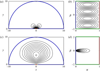
Comparison of small- $Pe$ optimal flows in an annulus with fixed kinetic energy (a,b,e,f,i,j) and fixed enstrophy (c,d,g,h,k,l). The outer boundary radius is $R=20$ (a–d), 100 (e–h) and 1000 (i–l). The fixed-kinetic-energy flows are shown in (a,e,i) in the $(\unicode[STIX]{x1D6FC},\unicode[STIX]{x1D6FD})$ plane and in (b,f,j) in the $(x,y)$ plane. The fixed-enstrophy flows are shown in (c,g,k) in the $(x,y)$ plane and in (d,h,l) in the $(\unicode[STIX]{x1D6FC},\unicode[STIX]{x1D6FD})$ plane.

We now discuss the solutions to the small- $Pe$ eigenvalue problem with fixed enstrophy for the annular domains with various outer radii $R$ . In figure 10(c,g,k), we present the optimal flows at $R=20$ (c), 100 (g) and 1000 (k) in the $(x,y)$ plane. When lengths are scaled by $R$ , the flows converge to a common solution in the large- $R$ limit, consisting of a smooth vortex dipole which is the size of the domain (and obeys no-slip at the boundaries). Physically, the higher derivatives acting on $\unicode[STIX]{x1D713}$ in (7.1) and (7.2) favour larger-scale flow structures. In (d,h,l), the same flows are shown in the $(\unicode[STIX]{x1D6FC},\unicode[STIX]{x1D6FD})$ plane. As $R$ increases (moving from (d) to (l)), the vorticity moves towards $\unicode[STIX]{x1D6FC}=0$ , where $h=R^{1-\unicode[STIX]{x1D6FC}}\log R$ is largest. In (b,f,j), we plot the optimal flows with fixed kinetic energy. In these cases, the vortex dipole is stretched towards the inner cylinder, with each vortex centre at a distance ${\sim}\sqrt{R}$ from the origin. In (a,e,i), the same flows are shown in the $(\unicode[STIX]{x1D6FC},\unicode[STIX]{x1D6FD})$ plane, where they become identical under a rescaling of the $\unicode[STIX]{x1D6FD}$ axis.

With fixed kinetic energy, we have larger vorticity near the inner cylinder. This vorticity is spread more uniformly in the fixed-enstrophy solutions. We now show that for these flows (i.e. (c,g,k)), the kinetic energy diverges in the limit of large $R$ . For the fixed-enstrophy flows, we have $\iint (\unicode[STIX]{x1D6E5}_{x,y}\unicode[STIX]{x1D713})^{2}\,\text{d}A=Pe^{2}$ . Thus, $(\unicode[STIX]{x1D6E5}_{x,y}\unicode[STIX]{x1D713})^{2}R^{2}\sim Pe^{2}$ , so $Pe/R\sim \unicode[STIX]{x1D6E5}_{x,y}\unicode[STIX]{x1D713}\sim \unicode[STIX]{x1D713}/R^{2}$ . Thus, $\unicode[STIX]{x1D713}\sim R$ and $\boldsymbol{u}=-\unicode[STIX]{x1D735}_{x,y}^{\bot }\unicode[STIX]{x1D713}\sim \mathbf{1}$ . Thus, the flow speed is of order 1 over an area ${\sim}R^{2}$ , so the kinetic energy diverges as $R^{2}$ as $R$ becomes large.

Figure 11.

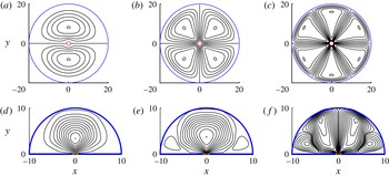
Comparison of small- $Pe$ optimal flows with fixed kinetic energy (a,b) and fixed enstrophy (c,d) in a half-disk with radius 10 above a heated plate of unit length centred at the origin. Optimal flow with fixed kinetic energy in the $(x,y)$ plane (a) and the $(\unicode[STIX]{x1D6FC},\unicode[STIX]{x1D6FD})$ plane (b). Optimal flow with fixed enstrophy in the $(x,y)$ plane (c) and the $(\unicode[STIX]{x1D6FC},\unicode[STIX]{x1D6FD})$ plane (d). Here, we use $\unicode[STIX]{x1D6FD}_{min}=-2$ , $\unicode[STIX]{x1D6FD}_{max}=2$ .

For the optimal flow over a heated plate in § 3, the domain is infinite. We have $h=(\unicode[STIX]{x03C0}/2)(\cosh (\unicode[STIX]{x03C0}\unicode[STIX]{x1D6FD})-\cos (\unicode[STIX]{x03C0}\unicode[STIX]{x1D6FC}))^{-1}$ . As $(\unicode[STIX]{x1D6FC},\unicode[STIX]{x1D6FD})\rightarrow (0,0)$ , $h\sim \Vert (\unicode[STIX]{x1D6FC},\unicode[STIX]{x1D6FD})\Vert ^{-2}$ . Thus, the small- $Pe$ eigenvalue problem is singular. Solving the problem numerically in the $(\unicode[STIX]{x1D6FC},\unicode[STIX]{x1D6FD})$ rectangle, we find that the solutions have unbounded kinetic energy and do not satisfy $\unicode[STIX]{x1D713}\rightarrow 0$ as $(\unicode[STIX]{x1D6FC},\unicode[STIX]{x1D6FD})\rightarrow (0,0)$ (or $x+\text{i}y\rightarrow \infty$ ). To examine the situation further, we consider a regularized version of the problem, in which the domain is cut off by a large semi-circle of radius $R$ on which $T=0$ (see figure 11 a). We compute $\unicode[STIX]{x1D6FC}$ and $\unicode[STIX]{x1D6FD}$ for this domain by modifying the unbounded definition (3.2a,b ),

We have added a power series, which gives a general representation of an analytic function which converges inside the disk of radius $R$ . We truncate the series at $k=N$ and choose the $a_{k}$ so that the $\sin k\unicode[STIX]{x1D703}$ components of $\unicode[STIX]{x1D6FC}$ are zero on $|z|=R$ . We find that the $a_{k}$ converge rapidly to 0 with increasing $k$ , so just a few terms are needed to obtain ${\sim}10^{-12}$ precision for $R=10$ .

In figure 11, we compare the optimal flows with fixed kinetic energy and enstrophy in the small- $Pe$ limit with $R=10$ . The flow with fixed kinetic energy (a) is almost identical to that in the unbounded case (figure 4 a), because the flow is very weak far from the plate in that case. Panel (b) shows the same flow in the $(\unicode[STIX]{x1D6FC},\unicode[STIX]{x1D6FD})$ plane. The optimal flow with fixed enstrophy (c) has a single vortex whose size is roughly that of the domain. Panel (d) shows this flow in the $(\unicode[STIX]{x1D6FC},\unicode[STIX]{x1D6FD})$ plane. The vorticity is concentrated near $(\unicode[STIX]{x1D6FC},\unicode[STIX]{x1D6FD})=(0,0)$ , where $h$ is largest.

Figure 12.

Transition from small- to large- $Pe$ optimal flows with fixed enstrophy for the annulus ( $R=20$ ) (a,b,c) and the bounded heated plate domain (d,e,f). For the annulus, $Pe=3.8$ (a), 27.9 (b) and 192 (c). For the heated plate, $Pe=3.8$ (d), 29.2 (e) and 213 (f), with $\unicode[STIX]{x1D6FD}_{min}=-2$ and $\unicode[STIX]{x1D6FD}_{max}=2$ .

In figure 12, we show how the optimal flows change as $Pe$ increases for the annulus ( $R=20$ ) (a,b,c) and the bounded heated plate domain (d,e,f). We compute the flows using a Newton solver for the nonlinear system of equations, similar to that described by Hassanzadeh et al. (Reference Hassanzadeh, Chini and Doering2014). In both domains, the trends are qualitatively similar to what was reported for the horizontal layer by Hassanzadeh et al. (Reference Hassanzadeh, Chini and Doering2014) with free-slip boundary conditions, and by Souza (Reference Souza2016) with no-slip boundary conditions. As $Pe$ increases, the convection rolls increase in number and become narrower. The flows become faster near the hot and cold boundaries, indicating the emergence of a boundary layer structure.

In summary, the optimal flows with fixed enstrophy have vortices that are much larger in scale than those for flows with fixed kinetic energy. In the examples shown here, the fixed-enstrophy flows are of the same size as the physical domain, while the fixed-energy flows are of the order of the size of the hot surface.

8 Summary and possible extensions

We have shown that a certain class of optimal flows for heat transfer can be generalized to a wide range of geometries using a change to conformal coordinates. The simplification occurs because the equations describing the optima involve conformally invariant differential operators (such as the Laplacian). The same approach has been used previously to simplify similar equations involving advection and diffusion (Boussinesq Reference Boussinesq1902; Choi et al. Reference Choi, Margetis, Squires and Bazant2005), such as those describing electrochemical transport (Bazant Reference Bazant2004; Bazant & Crowdy Reference Bazant and Crowdy2005).

We presented solutions in three basic situations: the exterior cooling of a cylinder, a hot flat plate embedded in a cold surface, and a channel with hot interior and cold exterior. Steady 2D flows were sufficient to present the basic idea, but unsteady flows can be addressed by retaining the unsteady term in the advection–diffusion equation. It seems likely that the coordinate change would be useful in certain 3D geometries as well, although these problems have not yet been solved. The simplest 3D cases would be those for which the boundary geometry is essentially uniform in the third ( $z$ ) dimension, so that one can use the conformal coordinates to map the flow domain in $(x,y,z)$ to one that is a rectangular prism in $(\unicode[STIX]{x1D6FC},\unicode[STIX]{x1D6FD},z)$ . This would at least allow the use of a regular grid if the problem needs to be solved numerically. The 3D flow velocity cannot be written in terms of a scalar streamfunction only, so the equations and method of solution need to be altered.