1. Introduction
Optimal reinsurance has been a research topic for many authors, and there are a number of approaches to the topic. These include finding the optimal type of reinsurance arrangement, and, for a given type of reinsurance arrangement, finding the optimal retention level. There are various well-documented approaches to this latter problem. A first approach is to find a retention level that minimises a ruin probability or, as a proxy, maximises the adjustment coefficient. See, for example, Waters (Reference Waters1983), Centeno (Reference Centeno1986), Hesselager (Reference Hesselager1990) and Dickson & Waters (Reference Dickson and Waters1996). A second approach is to apply utility theory and to find a retention level that maximises the expected utility of an insurer’s wealth over a fixed time interval. See, for example, Borch (Reference Borch1990), Bowers et al. (Reference Bowers, Gerber, Hickman, Jones and Nesbitt1997) and references therein. A third approach is to consider a dynamic reinsurance arrangement when there are investments, and to find an optimal reinsurance level where the criterion for optimality is minimising the ruin probability. Examples of this approach include Hipp & Vogt (Reference Hipp and Vogt2003) who studied excess of loss reinsurance, and Schmidli (Reference Schmidli2004) who considered proportional reinsurance. More recent studies have focussed on the effect of reinsurance on risk measures; for example see Chi & Tan (Reference Chi and Tan2011) and references therein.
This literature largely discusses decision making for an insurer based on a single criterion (e.g. minimising a ruin probability). Exceptions are studies which consider both the insurer and the reinsurer. See, for example, Dimitrova & Kaishev (Reference Dimitrova and Kaishev2010) and Hürlimann (Reference Hürlimann2011). A general problem, not just related to insurance, is that an outcome that is optimal under one criterion is most likely not optimal under a second criterion. Insurance companies operate in complex environments with a variety of potentially competing interests, for example shareholders, policyholders and regulators. Although it is generally impossible to satisfy all competing interests, it is of interest to study decision making when taking account of more than one criterion. We are not aware of any actuarial papers dealing with optimal reinsurance under multiple, conflicting, criteria, and we seek to address this issue in this paper.
Our objective in this paper is to apply methods from multiple attribute decision making (MADM) to find optimal retention levels in a series of case studies, and to assess whether or not the approach provides reasonable solutions. In particular, our research question is the selection of an optimal retention level under competing criteria, given a form of reinsurance, subject to a ruin probability constraint. We use case studies as mathematical analysis is not possible under our framework.
The underlying model for our case studies is the classical risk model. We consider a surplus process {U(t)}t>0, with U(0)=u, under a reinsurance arrangement, given by
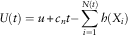 $$U(t)=u{\plus}c_{n} \:t{\minus}\mathop{\sum}\limits_{i=1}^{N(t)} h(X_{i} )\:$$
In this model, {N(t)}t≥0 is a Poisson process with parameter λ, and  $$\{ X_{i} \} _{{i=1}}^{\infty} $$
is a sequence of independent and identically distributed random variables, independent of {N(t)}t≥0, where X i represents the amount of the ith claim. We assume throughout that Pr(X 1<0)=0. Reinsurance applies to individual claims, and h(X i) denotes the net of reinsurance amount paid by the insurer on the ith claim, with 0≤h(X i)≤X i. The insurer’s net of reinsurance premium income per unit time is
 $$c_{n} =(1{\plus}\theta )\lambda \:E\:[X_{i} ]{\minus}(1{\plus}\xi )\lambda \:E\:[X_{i} {\minus}h(X_{i} )]$$
where θ and ξ are the premium loading factors used by the insurer and the reinsurer, respectively, and we assume that ξ>θ. We further assume that the net of reinsurance premium income is received continuously at rate c n per unit time. We impose the condition c n≥λE[h(X 1)] so that the insurer’s expected profit per unit time is non-negative. The finite time ruin probability is denoted by  $$\psi \left( {u,\,t} \right)$$
where
 $$\psi (u,\,t)={\rm Pr}(U(\tau )\,\lt\, 0\:\;{\rm for}\;{\rm some}\;\:\tau ,\,\:0\,\lt\, \tau \leq \,t\:\,\mid\,\:U(0)=u)$$
Now suppose that the insurer is subject to the regulatory constraint that the insurer’s initial surplus must be such that  $\psi \left( {u,\,t} \right)={\varepsilon}$
for a given time horizon, t, and appropriately small ε, say 1%. Let U be the initial surplus which satisfies this constraint in the absence of reinsurance (i.e. when h(X i)=X i). We refer to U as the maximum initial surplus. Our aim is to construct a set of pairs comprising initial surplus and retention level with the common feature that the initial surplus is less than U and the retention level is such that the ruin probability is ε. (Thus, from a solvency/ruin theory perspective, all pairs satisfy the same risk measure and so no pair is preferable to any other.) For each of these pairs, say (u j, R j), where u j is the initial surplus and R j is the retention level for the jth pair, we can compute the following measures:
1. Released capital: U−u j. By effecting reinsurance, the insurer can allocate this amount to other parts of its business. We assume that this allocation takes place immediately, so that the initial surplus becomes u j.
2. Expected profit at time t: (c n−E[h(X 1)])t. This amount depends on the form of reinsurance, h, and the retention level, R j.
3. Expected utility of wealth at time t: E[u(U(t))], where u is a utility function.
So, for the pair (u j, R j) we can calculate three numerical values under each of the above criteria, which we refer to as attributes, denoted (d j1, d j2, d j3). These are the inputs we will use in section 4 where we apply the MADM techniques described in section 3.
It should be clear from the descriptions above of our attributes that if we applied them in isolation, we would obtain contrasting outcomes. For example, due to our assumption that ξ>θ, the decision which maximises expected profit per unit time is to set h(X i)=X i. However, this decision results in the minimum release of capital (i.e. 0).
Our choice of attributes is inevitably subjective, and other attributes could be considered. For example, we could calculate conditional tail expectation for each pair. However, experiments with calculation of this quantity led to attribute values with similar characteristics to expected profit. Our choice of attributes results in outcomes that are different in nature, and measured on different scales (as illustrated in Figure 2).
Our aim in formulating the problem is twofold. First, we are interested in the effect of conflicting decision criteria. Second, we have tried to set the problem in a context that is neutral to both policyholders and the regulator. From the policyholders’ viewpoint, premiums charged and the probability of receiving claim payments are unaffected by the retention level. Likewise, from the regulator’s viewpoint, the retention level does not affect the ruin probability. The decision criteria affect only the insurer, and the retention level is based on the insurer’s preferences amongst the different criteria.
This paper is set out as follows. In section 2, we explain how we calculate ruin probabilities and values under our three criteria. In section 3, we give a summary of the techniques from MADM that we apply, and we discuss some issues as they relate to our problem. In section 4, we present our case studies and illustrate our approach in the case of two individual claim amount distributions, exponential and Pareto, which we have chosen because of their different tail behaviour. We consider two kinds of reinsurance: excess of loss, with h(X)=min(X, M), where M>0, and proportional, with h(X)=pX for 0<p≤1. We present and discuss some case studies in section 4 and provide some further analysis in section 5, then make some concluding remarks in section 6.
2. Calculation Methods
2.1. The translated gamma process
Dufresne et al. (Reference Dufresne, Gerber and Shiu1991) introduced the gamma process to the risk theory literature. Specifically, if a process {S G(t)}t>0 is a gamma process with parameters αt and β, then  $$S_{G} (t)\,\sim\,\gamma (\alpha t,\,\beta )$$
for all t>0. When α=β=1, the process is referred to as a standardised gamma process, denoted {S SG(t)}t>0. Dufresne et al. (Reference Dufresne, Gerber and Shiu1991) considered the surplus process {U G(t)}t>0 given by
 $$U_{G} (t)=U_{G} (0){\plus}ct{\minus}S_{G} (t),\quad t\,\gt \,0$$
with U G(0)=u. They showed how to calculate ultimate ruin probabilities for this risk process by calculating ruin probabilities when the aggregate claims process is a standardised gamma process, and by using a scaling argument to develop a simple relationship between ultimate ruin probabilities for a gamma process and those for a standardised gamma process.
Dickson & Waters (Reference Dickson and Waters1993) extended the work of Dufresne et al. (Reference Dufresne, Gerber and Shiu1991) in two ways. First, they gave formulae for the finite time ruin probability when the aggregate claims process is a standardised gamma process, and showed how these formulae could be used to calculate the finite time ruin probability when the aggregate claims process is a gamma process. Second, they introduced a translated gamma process {S TG(t)}t>0 defined by
 $$S_{{TG}} (t)=S_{G} (t){\plus}kt,\quad t\,\gt\, 0$$
where k is a constant. They showed that the finite time ruin probability when the aggregate claims process is a translated gamma process can be calculated from their formulae (2.3) and (2.4) for the finite time ruin probability when the aggregate claims process is a gamma process by a simple change to the premium rate. A major objective in Dickson & Waters (Reference Dickson and Waters1993) was to use ruin probabilities for translated gamma processes as approximations to ruin probabilities for the classical risk process, and they showed that this approach led to very good approximations. The idea behind the approximation was to match the first three moments of the compound Poisson (aggregate claims) process with those of the translated gamma process.
The ideas in Dickson & Waters (Reference Dickson and Waters1993) were applied by the same authors to the problem of calculating ruin probabilities under excess of loss and proportional reinsurance arrangements. Dickson & Waters (Reference Dickson and Waters1996) approximated compound Poisson processes under reinsurance by translated gamma processes. The great advantage of this approach is that ruin probabilities (in finite or in infinite time) can be approximated. The general problem with calculating ruin probabilities under reinsurance arrangements, particularly excess of loss, is that few explicit results exist. Dickson & Waters (Reference Dickson and Waters1996) illustrated that their translated gamma approximations work well in the few cases where approximations can be compared with exact values. In this paper, we therefore make the assumption that we can obtain a good approximation to the probability of ruin in finite time for a classical risk process under reinsurance by approximating the (net of reinsurance) aggregate claims process by a translated gamma process.
2.2. Calculation of the pairs (u j, R j)
We now assume that the ruin probability is fixed, that the type of reinsurance arrangement is known (so that we can calculate the parameters for the translated gamma approximation), and that the premium loading factors θ and ξ and the time period, t, are all fixed. The first step in constructing our set of pairs {(u j, R j)} is to find the maximum initial surplus U such that  $\psi \left( {U,\,t} \right)={\varepsilon}$
. There is no analytic way to find U. We simply find this numerically using a grid search. We then find the smallest value u s, say, such that the ruin probability is ε under reinsurance – again we use a numerical search. We then consider values of u s+jδ for a small value δ (illustrated in section 4) and positive integer j subject to u s+jδ<U. For initial surplus u s+jδ, we perform a numerical search for the retention level that results in a ruin probability of ε. This gives us a finite set of pairs {(u j, R j)} for which we can calculate individual values under our three attributes. The choice of δ is somewhat arbitrary. Ideally, we would like to perform our analysis based on a representative set of pairs and in all our case studies in section 4 we believe we have achieved this. Creating a larger set, for example, by switching from δ to δ/2, does not have any real effect on our overall analysis. In all our case studies we have used the same value of δ. As the values of u s and U depend on the premium loading factors, the time horizon and the claim size distribution, the number of pairs in a set varies.
Figure 1 shows a set of 252 pairs based on exponentially distributed individual claim amounts (with mean 1) and excess of loss reinsurance. (We discuss this case further in sections 4 and 5.) This is fairly typical of the sets of pairs we analysed for excess of loss reinsurance, with retention levels increasing with initial surplus. In this illustration, U=45.855 and the largest u j value is 45.850.
A set of pairs (u j, R j).

Depending on the loading factors θ and ξ, in some cases we found that there were two retention levels which resulted in a ruin probability of ε. We always chose the higher retention level as this results in a higher value for both expected profit and expected utility. Further, in these cases we conducted analysis based on two sets of pairs {(u j, R j)}, where the {R j} were increasing in one case and decreasing in the other. We found that the optimal pair was the same in each case.
An alternative method of selecting values of initial surplus (and hence pairs) would be to consider U, U−h, U−2h, …. A technical reason for taking our approach is that when there is no reinsurance, the attribute expected utility may not exist in the underlying compound Poisson model if the moment generating function of the individual claim amount distribution does not exist, even though the required calculation is possible under the translated gamma approximation. This consideration applies in section 4.1.2.
2.3. Calculation of attribute values
We now explain how we calculated values under each of our three attributes. Given a pair (u j, R j) and a maximum initial surplus U, the calculation of released capital is trivial as U−u j. Similarly, calculation of expected profit per unit time is straightforward based on our underlying classical risk model. We can perform calculations this way even though we are approximating the aggregate claims process by a translated gamma process as the approximation is based on moment matching. To calculate expected utility of wealth at time t, we need to specify a utility function. We adopt an exponential utility function u(x)=1−e −Bx, where B>0. Such utility functions are commonly used in the actuarial literature. One of its main advantages is that u(x) is defined for −∞<x<∞. One of its main disadvantages is that we require the existence of the moment generating function of the (net of reinsurance) aggregate claim amount random variable, although this is not an issue in our case studies in section 4 for reasons discussed at the end of the previous sub-section. It is straightforward to show that under this utility function, with the aggregate claims process approximated by a translated gamma process
 $$\:E\:[{\bf u}(U(t))]=1{\minus}{\rm exp}\{ {\minus}B(U(0){\plus}(c_{n} {\minus}k)t)\} \left( {{\beta \over {\beta {\minus}B}}} \right)^{{\alpha t}} $$
provided that B<β. (We remark that in applying this expression for the pair (U j, R j), each of α, β, k and c n depends on R j, and U(0)=u j.) The choice of an exponential utility function is not crucial to our analysis. The main point of this attribute is that it produces numerical outcomes that are on a very different scale to the other two attributes. However, there is one important point to make about the utility function. Application of the utility function  $${\tilde {\bf u}}(x)={\minus}e^{{{\minus}Bx}} $$
leads to the same decision as application of our utility function u under the expected utility criterion. See, for example, Bowers et al. (Reference Bowers, Gerber, Hickman, Jones and Nesbitt1997). The choice of utility function matters in our setting, for reasons that we explain in section 3. However, if we assume the insurer has a utility function, then this is not an issue.
Figure 2 shows values of our three attributes for the set of pairs in Figure 1. The numbers on the x-axis indicate the 252 pairs from Figure 1, with pair 1 being the point corresponding to the lowest initial surplus in Figure 1 and pair 252 corresponding to the highest initial surplus. The primary y-axis shows values for released capital (the decreasing function) and the expected profit (the lower increasing function). The secondary y-axis shows values for expected utility (the higher increasing function). This plot exhibits the main differences between the attribute values. Outcomes increase with initial surplus under two of the attributes, and decrease under the third, and outcomes are measured on different scales. The differences in the nature of the attribute values will be dealt with by the measure we calculate to select the optimal retention level. As an example of a difference, released capital represents funds available to the insurer at time 0, while, whatever the profit, accrues will only be known (and available) at time t. It is tempting to think that we should therefore consider some form of discounting, but this is not necessary. Multiplying every calculated value of expected profit by a discount factor like v t amounts to nothing more than scaling attribute values, which has no effect on the analysis, as explained in section 3.
Outcomes corresponding to pairs in Figure 1.
As an aside, we remark that in Figure 2, expected utility is increasing with initial surplus. Thus, the constraint of a fixed ruin probability leads to the conclusion here that under the single criterion of maximising expected utility, no reinsurance is the optimal strategy. This contrasts with applying utility theory without a constraint on ruin probability. See, for example, Dickson (Reference Dickson2005). We observed this in other calculations involving excess of loss reinsurance, but not proportional reinsurance.
3. MADM
In order to keep this paper relatively self-contained for an actuarial audience, we now give a brief description of the techniques we use in section 4 to find optimal retention levels. There is a large body of work on decision-making techniques, and a description of different approaches, including their pros and cons, can be found in Hwang & Yoon (Reference Hwang and Yoon1981) and Rao (Reference Rao2007). For our analysis we have selected a technique called TOPSIS that has been applied frequently in the decision theory literature and is suitable for use with purely numerical data.
In most studies, the TOPSIS method is identified as the best method among the MADM methods. According to Kim et al. (Reference Kim, Park and Yoon1997), the TOPSIS method has the following advantages over the other MADM methods: it has “(1) a sound logic that embodies the rationale of human choice, (2) a scalar value that considers the best and worst alternatives simultaneously, and (3) a simple computation procedure that can be easily programmed”. Rao (Reference Rao2007) states that the TOPSIS method provides a solution which is “not only closest to the hypothetically best, but is also the farthest from the hypothetically worst”. Velasquez & Hester (Reference Velasquez and Hester2013) describe advantages of TOPSIS as it being a simple process, that it is easy to use and to programme, and that the number of steps remains the same regardless of the number of attributes.
3.1. TOPSIS
TOPSIS is the acronym for Technique for Order of Preference by Similarity to Ideal Solution. Hwang & Yoon (Reference Hwang and Yoon1981) present it as a method to determine the best alternative based on the concept of a compromise solution. The compromise solution can be regarded as choosing the solution with the shortest Euclidean distance from the ideal solution and the farthest Euclidean distance from the negative ideal solution. In our context, the positive ideal points are equal to the maximum (weighted) value under each attribute, and the negative ideal points are equal to the minimum (weighted) value under each attribute. The ranking of the alternatives is based upon relative proximity to the ideal solution. Hwang & Yoon (Reference Hwang and Yoon1981: 129) give a pictorial representation of the situation in the case when there are two attributes.
In the decision theory literature, the TOPSIS method is the most popular decision-making technique. Examples of financial studies include Wu & Olson (Reference Wu and Olson2006) who presented a set of loan cases from Canadian banking for credit scoring using the TOPSIS method with 12 attributes depending on assets, earnings, equity and tax, and Hosseini et al. (Reference Hosseini, Ezazi, Heshmati and Moghadam2013) who explored the relationship between ranking of the top 50 listed companies on the Tehran Stock Exchange for the years 2009–2011 in terms of their liquidity, operation, leverage and profitability ratios.
We now describe briefly the steps to apply the method. A full description can be found in Hwang & Yoon (Reference Hwang and Yoon1981) and Rao (Reference Rao2007). Suppose that D is a decision matrix and there are m alternatives A 1, A 2, … , A m and n decision attributes C 1, C 2, … , C n. Let d ij denote the attribute value of A i on C j for i=1, 2, … , m and j=1, 2, … , n in the decision matrix D. (For example, in Figure 2, m=252 and n=3.) The steps are as follows.
1. Normalise the decision matrix as
where r ij is the normalised value, for i=1, 2, … , m and j=1, 2, … , n. We remark that this step explains why scaling attribute values does not affect the analysis – multiplication of each d ij by a constant does not change the normalised value r ij. This step also explains why different utility functions that give the same decision under the expected utility criterion will give different decisions when we apply TOPSIS. If we define $$r_{{ij}} ={{d_{{ij}} } \over {\sqrt {\mathop{\sum}\limits_{i\,=\,1}^m d_{{ij}}^{2} } }} $$
$$\tilde{d}_{{ij}} =d_{{ij}} {\minus}1$$
then (in an obvious notation)
$$\tilde{r}_{{ij}} \,\ne\,r_{{ij}} $$
.
2. Calculate weighted normalised values by using a weight vector ω=(ω 1, ω 2, … , ω n) as V ij=ω jr ij, for i=1, 2, … , n and j=1, 2, … , m. The weights are 1/n if we are giving equal weight to each attribute.
3. Construct the vectors of positive ideal points and negative ideal points, denoted
and
$$S^{{\plus}} =\left\{ {S_{1}^{{\plus}} ,\,S_{2}^{{\plus}} ,\:\,\ldots\!,\,S_{n}^{{\plus}} } \right\}$$
respectively.
$$S^{{\minus}} =\left\{ {S_{1}^{{\minus}} ,\,S_{2}^{{\minus}} ,\:\,\ldots\!,\,S_{n}^{{\minus}} } \right\}$$
4. Calculate the Euclidean distances between each alternative and the positive and negative ideal points. The distance between alternative A i and the positive ideal points is
and the distance between alternative A i and the negative ideal points is
$$\delta _{i}^{{\plus}} =\sqrt {\mathop{\sum}\limits_{j=1}^n (V_{{ij}} {\minus}S_{j}^{{\plus}} )^{2} } , \:\;{\rm for}\;i=1,\,2,\:\,\ldots\!,\,m$$
$$\delta _{i}^{{\minus}} =\sqrt {\mathop{\sum}\limits_{j=1}^n (V_{{ij}} {\minus}S_{j}^{{\minus}} )^{2} } , \:\;{\rm for}\;i=1,\,2,\:\,\ldots\!,\,m$$
5. Calculate the relative closeness of each alternative to the ideal solution as
so that C i∈[0, 1].
$$C_{i} ={{\delta _{i}^{{\minus}} } \over {\delta _{i}^{{\plus}} {\plus}\delta _{i}^{{\minus}} }}, \;{\rm for}\;i=1,\,2,\:\,\ldots\!,\,m$$
6. Rank the results according to the value of C i. The higher the ranking, the better a solution is.



Velasquez & Hester (Reference Velasquez and Hester2013) explain that the disadvantages of TOPSIS include that the use of Euclidean distance does not consider the correlation of attributes, and the choice of weights is subjective. However, the issue of correlation can be addressed by the use of a different distance measure, which we now describe.
3.2. TOPSIS with Mahalanobis distance
In Figure 2, we see that there are various relationships between the different outcomes. For example, a low value of released capital results in a high value of expected profit. Antucheviciene et al. (Reference Antucheviciene, Zavadskas and Zakarevivius2010) discuss the situation when attributes are dependent and suggest an alternative measure of distance called Mahalanobis distance or quadratic distance, originating from Mahalanobis (Reference Mahalanobis1936). They state that “when alternatives are described by statistically connected criteria, application of TOPSIS based on Euclidean distances can lead to inaccurate estimation of relative significances of alternatives and cause the improper ranking results”. To allow for dependence, distance is measured using a covariance matrix. Let Σ be the covariance matrix for our normalised attribute values, and let ω be a set of weights (as in Step 2 in section 3.1). Let Ω be a diagonal matrix defined as  $$\Omega ={\rm diag}\,(\sqrt {\omega _{1}} ,\,\sqrt {\omega _{2}} ,\:\,\ldots\!,\,\sqrt {\omega _{n}} )$$
, and for i=1, 2, … , m, let (S j+−r ij) be a column vector with n rows. The Mahalanobis distance between alternative A i and the positive ideal points is
 $$\Delta _{i}^{{\plus}} =\sqrt {(S_{j}^{{\plus}} {\minus}r_{{ij}} )^{T} \:\Omega ^{T} \:\Sigma ^{{{\minus}1}} \:\Omega \:(S_{j}^{{\plus}} {\minus}r_{{ij}} )} \;{\rm for}\;i=1,\,2,\:\,\ldots\!,\,m$$
and the Mahalanobis distance between alternative A i and the negative ideal points is
 $$\Delta _{i}^{{\minus}} =\sqrt {(S_{j}^{{\minus}} {\minus}r_{{ij}} )^{T} \:\Omega ^{T} \:\Sigma ^{{{\minus}1}} \:\Omega \:(S_{j}^{{\minus}} {\minus}r_{{ij}} )} \;{\rm for}\;i=1,\,2,\: \ldots\!,\,m$$
where S + and S − are as in section 3.1, except that they are based on the unweighted r ij. With these measures we then proceed as in Steps 5 and 6 in section 3.1, with the relative closeness now being calculated as
 $$C_{i} ={{\Delta _{i}^{{\minus}} } \over {\Delta _{i}^{{\minus}} {\plus}\Delta _{i}^{{\plus}} }} \;{\rm for}\;i=1,\,2,\:\,\ldots\!,\,m$$
For all calculations in the following section, we have used sample variance and sample covariance in Σ as the pairs that we are using for each combination of time and loading factors are just a sample from the population of possible pairs resulting in a ruin probability of ε.
4. Case Studies
Our analysis is based on case studies. We do this because mathematical analysis of our problem does not seem possible. In particular, it does not seem possible to obtain pairs (u j, R j) without making assumptions about the form of reinsurance or the individual claim size distribution. Our (net of reinsurance) aggregate claims process is approximated by a translated gamma process. Specifically, for a reinsurance arrangement h, the parameters of this process are given by
 $$\alpha ={{4\lambda \:E[h(X_{1} )^{3} ]} \over {E[h(X_{1} )^{2} ]}},\:\,\quad\beta ={{2E[h(X_{1} )^{2} ]} \over {E[h(X_{1} )^{3} ]}},\quad\,k=\lambda \left( {E[h(X_{1} )]{\minus}{{2E[h(X_{1} )^{2} ]} \over {E[h(X_{1} )^{3} ]}}} \right)$$
(See Dickson & Waters, Reference Dickson and Waters1993.) It seems highly unlikely to the authors that there exist many random variables, say Y and Z, whose distributions are suitable models for individual claim amounts, that satisfy E[h(Y)r]=E[h(Z)r] for r=1, 2, 3 and for all possible retention levels under the rule h. The only case that we can identify is when the first three moments of Y and Z are identical and when h(x)=px, where 0<p≤1 (i.e. proportional reinsurance). Consequently, it does not seem possible to obtain distribution-free results given h. Similarly, given an individual claim amount distribution, we cannot calculate the parameters α, β and k, and hence ruin probabilities and attribute values, without specifying h.
Our case studies are based on two types of reinsurance – excess of loss and proportional – and two individual claim amount distributions with mean 1 – exponential, as an example of a light-tailed distribution, and Pareto(4,3) as an example of a heavy-tailed distribution.
Throughout this section we assume that the Poisson parameter is 500 per unit of time, and we consider four pairs of premium loading factors (θ, ξ), namely (0.1, 0.15), (0.1, 0.2), (0.1, 0.3) and (0.2, 0.3). The finite time ruin probability is 0.01, regardless of the time period, and our selected time periods are 0.1, 0.5, 1, 5, 10 and 20 years. Setting the same ruin probability regardless of the time period provides a basis for comparison of results. However, we could equally think of our calculations as representing a 1-year period with different volumes of business with the expected number of claims, respectively, being 50, 250, 500, 2,500, 5,000 and 10,000, in which case a regulatory ruin probability would be set regardless of volume of business. Finally, the parameter B of our utility function is 0.02. We discuss what happens when this parameter varies in section 5.2.
4.1. Excess of loss reinsurance
We start with excess of loss reinsurance, so that h(X)=min(X, M).
4.1.1. Exponential claims
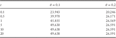
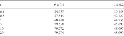
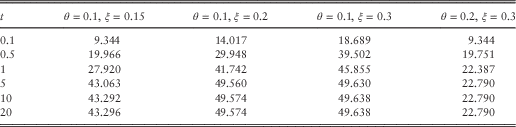
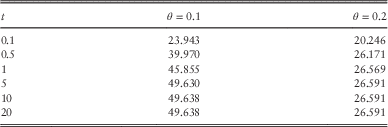
We first consider the situation when individual claims are exponentially distributed with mean 1. Table 1 shows values of u such that  $\psi \left( {u,\,t} \right)=0.0{\rm 1}$
for different values of t when there is no reinsurance. The reason why the values are unchanged going from t=10 to t=20 is that with the large value for the Poisson parameter, the finite time ruin probability for t=10 is very close to the ultimate ruin probability.
Values of u such that ψ(u, t)=0.01 when θ=0.1 and θ=0.2, exponential claims.
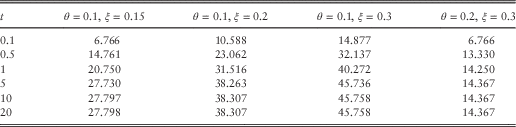
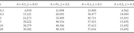
The next step is to calculate the smallest possible value of the initial surplus under reinsurance such that the finite time ruin probability is 0.01. Table 2 shows these values for our different combinations of θ and ξ.
Smallest initial surplus levels, exponential claims, excess of loss reinsurance.
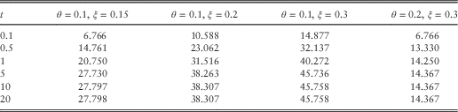
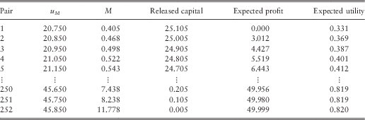
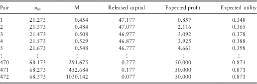
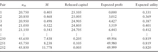
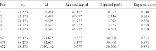
Thus, for example, in the case when t=1, θ=0.1 and ξ=0.15, we consider pairs (u M, M), where the smallest value of u M is 20.750. We have then considered values of u starting from 20.750 and increasing by 0.1 to 45.850 (as the largest possible initial surplus is 45.855 from Table 1), giving a set of 252 pairs. These pairs are shown in Figure 1, and the values of our three attributes are plotted in Figure 2. Table 3 shows some of the values underlying this plot. A feature in this table is that as the initial surplus increases, so does the retention level, and we observed this in our other calculations for excess of loss reinsurance.
Some values from Figure 2.
In the tables that follow, we calculate optimal pairs (u M*, M*) using the covariance matrix discussed in section 3. As an illustration of this matrix, we again consider the case when t=1, θ=0.1 and ξ=0.15. The covariance matrix is as follows, with the ordering of the rows being released capital, expected profit and expected utility:
 $$\left( {\matrix{ {0.0010} & {{\minus}0.0006} & {{\minus}0.0003} \cr {{\minus}0.0006} & {0.0004} & {0.0002} \cr {{\minus}0.0003} & {0.0002} & {0.0001} \cr } } \right)$$
It is important that a high degree of numerical accuracy is maintained in this matrix, as this can have a significant effect on the calculation of the inverse, and hence on the calculation of distance from the ideal points.
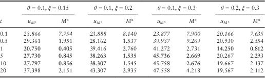
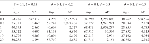
We also need to adopt a set of weights. Initially, we assume that equal weight attaches to each attribute, and Table 4 shows the optimal pairs using these weights. In this table we have used italic and bold font for certain meanings. If a pair is in italic font, it means that the value u M* is the largest value we considered for initial surplus (and so M* is the highest retention level considered), and if a pair is in bold font, it means that the value u M* is the smallest value we considered for initial surplus (and so M* is the lowest retention level considered).
The optimal pairs (u M*, M*), exponential claims.
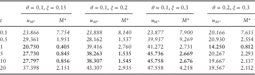
We note that there is no obvious pattern in Table 4. To understand why this is, we first make some comments about our attributes.
∙ For each set of outcomes analysed, there is a pair (u j, R j), where the value of u j is very close to U. Consequently, values for released capital run from close to 0 to a maximum value. Very high values of M* are effectively indicating that no reinsurance is the optimal strategy.
∙ For each set of outcomes analysed, expected profit increases to a maximum. However, depending on the combination of t, θ and ξ, the minimum value of expected profit may not be very close to 0. In such cases we have a contrast from released capital as the normalised values of expected profit are generally over a shorter interval.
∙ For each set of outcomes analysed, expected utility increases. However, for the larger values of t, particularly 10 and 20, values of expected utility are very close to 1 for all pairs (u j, R j) and so expected utility has virtually no effect on the choice of optimal pair.
Figure 3 shows plots of the normalised values for exponentially distributed claims for the case θ=0.1 and ξ=0.2 when t=0.1, 1, 5 and 20, shown from top left to bottom right. As the plots show normalised values, there is no need to have separate scales as in Figure 2. In each plot, the decreasing line represents released capital, whereas the increasing line with the lower starting point represents expected profit. We observe that as t increases, the line representing expecting utility flattens out, and in the cases t=1, 5 and 20, the minimum value for expected profit is not particularly close to 0.
Normalised values for exponential claims, excess of loss reinsurance.
It is worth commenting here that these figures may suggest that our normalisation is inappropriate as the normalised values have different ranges. Suppose that instead of working with {r ij} we had worked with the normalisation (called feature scaling)
 $$\hat{r}_{{ij}} ={{d_{{ij}} {\minus}d_{i}^{{\minus}} } \over {d_{i}^{{\plus}} {\minus}d_{i}^{{\minus}} }}$$
where d i− and d i+ are, respectively, the minimum and maximum of  $$\{ d_{{ij}} \} _{{j=1}}^{m} $$
, then all normalised values would be in the interval [0, 1]. However, this is just a different form of scaling and results in exactly the same {C i} values that are calculated using {r ij}. In other words, we reach the same conclusions. The normalisation we have used highlights the relative closeness of an attribute value to the positive and negative ideal points.
Figure 3 suggests that the attribute released capital will be more influential, at least for larger values of t where distances to positive and negative ideal points can be much greater than under the other two attributes.
In Table 4, we observe that for the smallest value of t (0.1), the optimal outcome for each combination of loading factors is effectively no reinsurance. This results in maximum values for expected profit and expected utility, but the minimum value (i.e. 0) for released capital. As each attribute has equal weight, it is not a great surprise that the optimal outcome is no reinsurance. Also, for this value of t, for each combination of loadings, the expected profit for the first alternative is very close to 0, meaning that the range of normalised values is greater. It is also true that the range of normalised values is greater for the attribute expected utility. However, as t increases, these comments no longer apply. For most of the remaining combinations of time and loadings in Table 4, the expected profit for the first alternative is very much greater than 0, and the range of normalised values for expected utility decreases similarly to what is shown in Figure 3.
We can also see that the optimal pairs in Table 4 reflect the different costs of reinsurance. For example, the optimal values of M* are higher for the combination 0.1/0.3 compared with the combination 0.2/0.3, reflecting the relatively higher cost of reinsurance.
In the case t=20, when expected utility is very close to 1 for all alternatives, if we perform the analysis based only on released capital and expected profit, the optimal pairs do not change much from those in Table 4.
4.1.2. Pareto claims
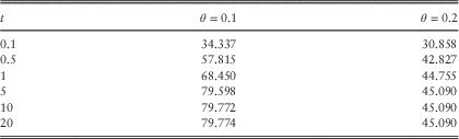
We now consider the situation when the individual claim amount distribution is Pareto(4,3). Like the exponential distribution in the previous section, this distribution has mean 1, but it is a heavy-tailed distribution, and so we might expect differences from the results in the previous section. Tables 5 and 6 show the same quantities as Tables 1 and 2, respectively.
Values of u such that ψ(u, t)=0.01 when θ=0.1 and θ=0.2, Pareto claims.
Smallest initial surplus levels, Pareto claims, excess of loss reinsurance.
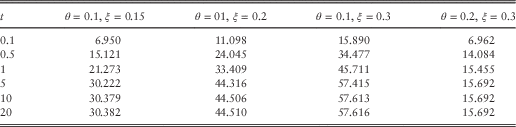
Comparing these tables with Tables 1 and 2 we see that the values of the maximum initial surplus are greater for Pareto claims, particularly when θ=0.1, and the smallest initial surplus levels are also generally greater for Pareto claims. Thus, when we again consider initial surplus levels increasing by 0.1 from the smallest initial surplus level (for a given combination of θ and ξ), we create larger sets of alternatives than in the case of exponentially distributed claims. However, as illustrated in Figure 4, where t=1, θ=0.1 and ξ=0.15, we see that the broad pattern of attribute values is similar to Figure 2. In this figure, the decreasing plot shows released capital, whereas the increasing plot with the lower starting point shows expected utility. Some values underlying this plot are shown in Table 7. Table 8 shows the optimal pairs (u M*, M*) when the weights are equal, and the italic and bold fonts have the same meaning as in Table 4.
Outcomes for Pareto claims, θ=0.1, ξ=0.15 and t=1, excess of loss reinsurance.
Some values from Figure 4.
The optimal pairs (u M*, M*), Pareto claims.
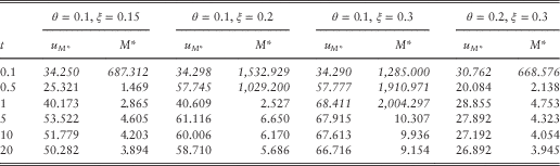
The situation in Table 8 is somewhat different to Table 4. For t=0.1 it is still the case that the optimal strategy is essentially no reinsurance. It is also true that for most combinations of time and loadings, the expected profit for the first alternative is very much greater than 0. However, unlike in Table 4, none of the optimal pairs in Table 8 is the alternative with the lowest initial surplus. If we compare Tables 1 and 2 with Tables 5 and 6 we see that the difference between the smallest initial surplus levels and the values of u that make  $\psi \left( {u,\,t} \right)=0.0{\rm 1}$
are larger in the case of Pareto claims. This creates a greater range of values for released capital and expected profit, and for the normalised values of these, which causes the difference from the exponential claims case.
4.2. Proportional reinsurance
We now consider proportional reinsurance. It turns out that results are less interesting than in the case of excess of loss reinsurance, and so we present results only for exponentially distributed individual claim amounts (with mean 1).
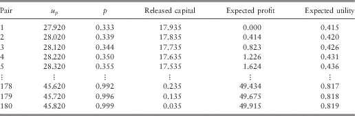
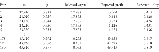
The values of u such that ψ(u, t)=0.01 when there is no reinsurance are the same as in Table 1 and values of the smallest initial surplus levels are shown in Table 9. Comparing Tables 1 and 9 we see that for some combinations of θ, ξ and t there is not a great difference between the smallest initial surplus and the maximum initial surplus, and in these cases it is not particularly meaningful to find optimal retention levels. Figure 5 illustrates the situation when θ=0.1, ξ=0.15 and t=1, and Table 10 shows some of the pairs (u p, p) underlying this figure. In this figure, the decreasing plot shows released capital, the higher increasing plot shows expected utility and the lower increasing plot shows expected profit. Although we are considering a different type of reinsurance, the patterns are similar to Figures 2 and 4.
Outcomes for exponential claims, θ=0.1, ξ=0.15 and t=1, proportional reinsurance.
Smallest initial surplus levels, exponential claims, proportional reinsurance.
Some values from Figure 5.
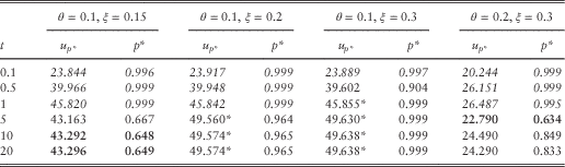
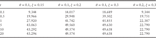
Following our approach for excess of loss reinsurance we calculate optimal pairs, denoted (u p*, p*), using the covariance matrix discussed in section 3.2. Table 11 shows the optimal pairs when equal weights are allocated to each attribute (corresponding to Table 4 for excess of loss reinsurance). In this table, if the value of u p* is marked with a *, then this means that we could only identify a single pair which gives a 1% ruin probability for that combination of loadings and time.
The optimal pairs (u p*, p*), exponential claims, proportional reinsurance.
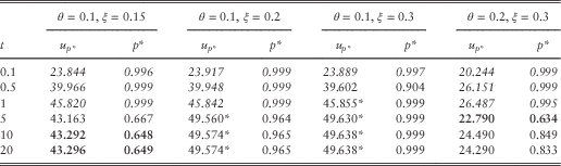
The major feature of Table 11 is that the optimal strategy is effectively no reinsurance for small values of t in Table 11, based on the increasing values under two of the attributes (as illustrated in Figure 5).
5. Further Analysis
5.1. The effect of the weights
Our analysis so far has been based on equal weights attaching to each attribute. We now consider what happens when weights vary. In the analysis that follows, we vary the weight, ω 1, attaching to released capital and set ω 2=ω 3=(1−ω 1)/2. What we would expect to happen in this situation is that the optimal retention level should be non-increasing, starting from the largest possible retention level when ω 1=0 and reducing to the smallest possible retention level when ω 1=1. Equivalently, the value of u M* should be non-increasing, resulting in higher levels of released capital as ω 1 increases.
Figures 6 and 7 show how u M* changes when t=0.5 and t=1, respectively, for the case θ=0.1 and ξ=0.2. The patterns in these figures are typical of what we observed with the optimal u (and hence M) being non-increasing with ω 1. When we removed the constraint ω 2=ω 3, but imposed ordering on ω 2 and ω 3, for example, ω 2=2ω 3, we observed similar patterns. What we observe here is that as the weight attaching to released capital increases, the optimal initial surplus does not increase, and for many values of ω 1 the optimal pair gives the minimum initial surplus and hence maximum released capital.
Optimal initial surplus when θ=0.1, ξ=0.2 and t=0.5 as ω 1 varies.
Optimal initial surplus when θ=0.1, ξ=0.2 and t=1 as ω 1 varies.
We observe a “discontinuity” in each figure. In the case of Figure 6, for small values of ω 1 the optimal solution is no reinsurance, which gives the maximum possible values for expected profit and expected utility. However, from ω 1=0.25 the weight attaching to released capital has an effect, resulting in decreasing values of both u M* and M*. In the case of Figure 7, we see that as ω 1 increases from 0, the effect is a decrease in both u M* and M*, and from ω 1=0.45 the outcome is the lowest possible initial surplus and maximum released capital. Although it might be mathematically more pleasing if the plots in Figures 6 and 7 displayed a steady decrease in the optimal initial surplus, the plots nevertheless have the key feature we would expect, that is non-increasing.
In summary, attribute 1 values decrease as the retention level increases, whereas the opposite is true for attributes 2 and 3. Increasing the weight on attribute 1 while decreasing the total weight on attributes 2 and 3 in a consistent ratio results in outcomes we would expect.
5.2. The effect of the utility function
In all calculations so far, the parameter of our utility function has been B=0.02. We have tested the effect of a 1% change in this parameter and found that in most cases we obtained the same optimal pair. In cases where we did not obtain the same optimal pair, the optimal pair was a neighbour to the optimal pair with B=0.02. (Here, by “neighbour” we mean that the value of is u M*±0.1, where u M* is the optimal value of u when B=0.02.) So, in a local sense, the outcomes do not seem to be very sensitive to the value of B.
We also experimented with larger changes to B, setting values from 0.015 to 0.025. For many combinations of time and loading factors we found that the value of B had no effect whatsover on the optimal pair. In cases where it did have an effect, it is difficult to draw general conclusions as the effect depends on a variety of factors including the weights.
5.3. Comparison with single attribute decision making
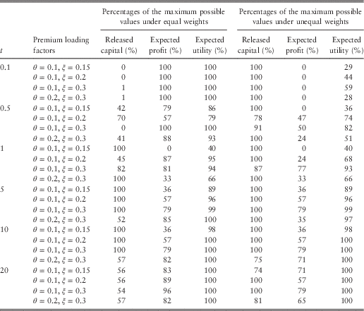
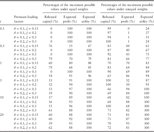
If we consider our three criteria individually, we can find the optimal retention level and calculate the attribute value at this optimal level. For example, under the criterion of maximising expected profit, the optimal retention level will be the highest possible. Our purpose in this section is to compare our outcomes at the optimal retention level with the optimal values under each of the three individual criteria. Tables 12 and 13 show values of released capital, expected profit and expected utility at the optimal pair as a percentage of the maximum possible value of each attribute for excess of loss reinsurance and exponentially and Pareto-distributed claim sizes, respectively. We have considered two cases; equal weights and weightings of 0.5/0.25/0.25.
Percentage of maximum possible value of each attribute under excess of loss reinsurance, exponential claims.
Percentage of maximum possible value of each attribute under excess of loss reinsurance, Pareto claims.
We have shown values for excess of loss reinsurance only as this is the more interesting case. Again, it is not easy to pick patterns in these tables. However, we can observe that the change of weights from equal to 0.5/0.25/0.25 results in the maximum release of capital in most cases, as we might expect. We also observe that many values for expected utility are 100%. There are two reasons for this. The first is that for small values of t, the attribute values (for expected utility) increase, and there is a reasonable range of values, as illustrated in the top left plot in Figure 3. Combined with increasing attribute values for expected profit, the optimal pair is the one with the highest retention level. For large values of t, values of expected utility change little. For example, we can see from the bottom right plot in Figure 3 that whichever pair (u j, M j) was chosen, the value of expected utility for this pair would be close to the maximum value.
The nature of our analysis is such that we are able to consider attributes with different ranges for their numerical values (through normalisation). As t increases, the range for expected profit increases, but the range for released capital does not. We can see in the case of equal weights that for large values of t the percentages for expected profit are high, particularly in the case of Pareto claims. This is a desirable feature. Intuitively, we would not want our approach to be producing optimal pairs which result in a large percentage of potential profit being sacrificed.
6. Concluding Remarks
We have chosen to investigate optimal retention levels in the context of conflicting decision criteria using a standard approach, and our case studies suggest that the TOPSIS technique produces sensible outcomes for optimal reinsurance arrangements. It is a fairly straightforward technique to apply, and, as we have seen, we can have some control over the outputs through the choice of weights for the different attributes. In terms of calculations, the most time-consuming part of this work was in the calculation of sets of pairs {(u j, R j)}. Programming in R, it took 24–36 hours to produce a set of pairs for a given pair of loading factors. The TOPSIS calculations can be done almost instantaneously.
The great advantage of the TOPSIS method is that we only need numerical input to perform our analysis. The disadvantage is that as TOPSIS is a numerical method, we cannot obtain mathematical expressions for optimal retention levels, which restricts our ability to analyse our results. Our analysis was based on specific types of insurance and specific claim size distributions. These were necessary to calculate sets of pairs {(u j, R j)} and ruin probabilities {ψ(u j, t)}. It does not seem possible to perform analysis based on unspecified claim size distributions or general forms of reinsurance arrangement. For example, finding the optimal type of reinsurance does not seem possible in our setting. We believe these observations would be true under simpler ruin probabilities, for example, 1-year discrete time ruin probabilities, or similar risk measures. We have performed analysis based on continuous time ruin probabilities as these are less time consuming to calculate than discrete time ones. However, such calculations are possible, and do not require any restriction on the premium principle.
It is not particularly surprising that the premium loading factors and the individual claim size distribution have an effect on outcomes, nor is it surprising that proportional reinsurance is less interesting than excess of loss reinsurance.
Our results are all based on sets of pairs {(u j, R j)} that we have chosen. Thus, unlike analysis based on a mathematical function, our results are not definitive, but are indicative of optimal retention levels. In actuarial practice, results based on any mathematical model or analysis are only part of the input into any decision, and our analysis should be seen in this light.
Acknowledgements
The authors would like to thank the associate editor and referee whose feedback greatly improved this paper. Başak Bulut Karageyik has been supported by the 2214/A-International Doctoral Research Fellowship Program-TÜBITAK during her studies at the University of Melbourne.