


The concept of spatial or proximity voting (Black Reference Black1948; Davis, Hinich, and Ordeshook Reference Davis, Hinich and Ordeshook1970; Downs Reference Downs1957; Hotelling Reference Hotelling1929) has been highly influential in the study of voting, elections, and political science generally. The central assumption of spatial voting theory is that a citizen will cast her vote for the candidate whose policy position is closest to her own views. This general framework has spawned a multitude of theories, arguments, and more elaborate models (both statistical and formal) to describe and account for voting behavior both in elections and in institutions such as Congress and the courts.
The spatial voting approach differs from the political behavior tradition of studying vote choice, which primarily emphasizes an attitude-driven model in which many factors work together to determine which candidate a citizen supports. Party identification (Campbell et al. Reference Campbell, Converse, Miller and Stokes1960), group membership (Lazarsfeld, Berelson, and Gaudet Reference Lazarsfeld, Berelson and Gaudet1952), personal financial situation (Sigelman and Tsai Reference Sigelman and Tsai1981), and policy views (Brody and Page Reference Brody and Page1972) all have important effects on vote choice.Footnote 1 The relevance of a given factor within the behavioral tradition is established by showing that it has a strong relationship with vote choice, either in terms of the magnitude of an effect or the amount of variance explained. The spatial voting tradition, in contrast, posits precise, albeit simplified, models of voting, focusing on the policy views of voters in relation to the positions of candidates. These models must then be validated by confirming specific criteria about the exact relationship between policy views and vote choice. In this way, the spatial voting approach trades the breadth and completeness of behavioral models for both precision and parsimony.
Strong tests of the spatial model require direct measurements of the positions of voters and candidates on the same scale. Until now, such measurements could be obtained only by making unrealistically strong assumptions about the information provided by standard survey measures. In this article, I propose a new measure that directly locates citizens and candidates in the same clearly defined ideological space. In particular, I measure the ideological locations of John Kerry and George W. Bush in the 2004 election based on their roll call voting in the U.S. Senate, and I measure the ideologies of voters based on their responses to survey questions asking how they would vote on 31 specific proposals, each of which was actually voted on in the Senate. This joint scaling reveals how close each respondent is to Kerry and Bush, allowing for direct examination of the criteria defined by spatial voting theories.
4pt Based on the analysis of this joint scaling, this article reports three main findings. The first is that the majority of citizens do have ideologically organized preferences on the types of proposals voted on in the U.S. Senate. This finding stands apart from other work on public opinion, which has generally measured mass attitudes by means of highly simplified or symbolic representations of public policy controversies. Second, I find that most voters rely heavily on candidate policy positions, as measured by the candidates’ actual political behavior, in choosing between Bush and Kerry. Third, I find that the behavior of some but not all voters is in close accord with the foundational axioms of the basic spatial voting model. Specifically, I find that the point at which independent voters switch from being more likely to vote for Kerry to being more likely to vote for Bush is located almost exactly at the midpoint between the two candidates’ positions. This is almost as true for low information independents as for those with higher information levels. Democratic and Republican voters, however, display systematic biases toward candidates of their own party above and beyond their relative ideological proximity to Bush and Kerry. The behavior of partisans converges toward the assumptions of unbiased spatial voting as information levels increase, but even the most informed partisans show significant biases by the spatial standard. On the whole, these results provide the strongest and most direct evidence to date on whether voters in real world elections do in fact adhere to the basic precepts of the spatial voting model.
A DIRECT TEST OF SPATIAL VOTING
This section establishes the baseline against which voting decisions will be judged. The approach is not unlike that used by Lau and Redlawsk (Reference Lau and Redlawsk1997) to determine whether citizens are “voting correctly.” Although these authors defined correct votes as those that would be unchanged if voters were to become fully informed, the standard used in this article is based on compatibility with the assumptions of the spatial voting model. I begin with a standard spatial voting setup for a two-candidate election. Because I focus on the 2004 presidential election, we have George W. Bush and John Kerry taking positions at θ and φ , respectively. Under perfect spatial voting, there would be a cutpoint midway between the two candidates at (θ + φ)/2. Every voter to the left of this cutpoint would be closer to Kerry than to Bush and, hence, would cast his vote for Kerry. Similarly, every voter to the right of the cutpoint would vote for Bush. Beyond this simple deterministic model, however, several lines of scholarship have broadened the spatial framework to accommodate nonpolicy factors that may impact voting decisions.Footnote 2 Unmeasured nonpolicy influences have been included in spatial models in order to describe the various forces that may operate on individual voters in making their voting decisions. These are generally modeled as random disturbances, representing the largely unsystematic differences between individuals’ feelings toward the candidates, personal experiences, or other quantities. Much of the work in this area has analyzed the theoretical consequences of allowing such random errors in voting (Adams Reference Adams1999; Enelow and Hinich Reference Enelow and Hinich1984; Hinich and Munger Reference Hinich and Munger1994; Lin, Enelow, and Dorussen Reference Lin, Enelow and Dorussen1999; Schofield Reference Schofield2002). When analyzing vote choice in real world elections, it is reasonable to use models that allow such errors to operate at the individual level, rather than testing a clearly incorrect model of perfect spatial voting in which no voter ever makes a “mistake” by spatial standards. Within this stochastic spatial voting setup, a sensible hypothesis to examine, then, is not whether voters perfectly follow the assumptions of deterministic (errorless) spatial voting, but instead whether people's decisions correspond to a model in which they vote on average according on their ideological proximity toward candidates.
The central assumption of spatial voting is that voters tend to choose the candidate whose position is closest to their own. A minimally necessary condition for this is that those with more conservative policy views be more likely to vote for the conservative candidate. Therefore, the first condition for spatial voting is that voters with more conservative ideologies should be more likely to vote for Bush than those with more liberal ideologies. Clearly, this is a necessary, but not sufficient, condition for spatial voting. It simply implies that people are using ideology in at least a directionally correct fashion. Beyond this first criterion, spatial voting also implies that as their ideology becomes more conservative, voters should switch from being more likely to vote for the liberal candidate to being more likely to vote for the conservative candidate when their ideal point passes the midpoint between the two candidates’ positions. If, for example, Kerry and Bush take positions at φ and θ, respectively, we have a midpoint between the two candidates at (θ + φ)/2. For spatial voting to take place, not only must conservatives be more likely than liberals to vote for Bush, but it must also be the case that respondents with ideal points at the midpoint between these two candidates’ positions be approximately indifferent between the two choices. This second condition can be thought of as an unbiasedness requirement for spatial voting. The use of the term “bias” here is not meant to have a normative connotation, but rather to draw parallels to the concept of bias of statistical estimators. This parallel is especially useful because we examine a stochastic version of spatial voting.
Figure 1 shows two examples of voting rules that people could use in order to make voting decisions based on their policy preferences. Both voting rules displayed pass the first test of spatial voting—that as people become more conservative, their probability of voting for the conservative candidate increases. In the left pane of Figure 1, an unbiased voting rule is shown. In this case, voters are indifferent between Bush and Kerry—having a 50% chance of voting for each—when their policy views fall at the actual midpoint between the two candidates’ positions. In the right pane, the curve depicts a biased voting rule in which the indifference point of respondents (the ideal point value at which a respondent would have an equal chance of voting for either candidate) falls well to the left of the true midpoint between the two candidates. As a consequence of this, respondents whose policy views fall at the actual midpoint between the two candidates are much more likely to vote for Bush than for Kerry. Furthermore, under this biased decision rule, voters whose ideal points fall in the shaded area of the graph will be ideologically closer to Kerry, but will have greater than a 50% chance of voting for Bush. This clearly violates the assumptions of unbiased spatial voting.
Examples of Possible Voting Rules

In addition to unmeasured (random) nonpolicy factors, some researchers have constructed spatial voting models that account for the effects of specific measured factors on vote choice in the spatial voting tradition. Some of these expanded models have included components such as valence dimensions, under which one candidate possesses an advantage based on personality, honesty, or some other characteristic that is valued equally by all voters (Ansolabehere and Snyder Reference Ansolabehere and Snyder2000; Groseclose Reference Groseclose2001; Stokes Reference Stokes1963). Other models allow voters to cast their ballots in part on nonpolicy dimensions on which citizen preferences may differ, such as party identification, ideological labels, or other concerns (Adams Reference Adams2001; Adams, Merrill, and Groffman Reference Adams, Merrill and Grofman2005; Chapman Reference Chapman1967, Reference Chapman1968). Directly modeling these factors rather than including them as random disturbances becomes particularly important when it is suspected that their values will be correlated with voter ideology, as in the case of factors such as party identification.Footnote 3
The analysis of spatial voting presented here seeks to determine whether the behavior of voters from each partisan identification follows the assumptions of spatial voting theory. This can also be thought of as a statistical test for the size of the nonpolicy influence of identifying with one of the two major parties, which would be equal to zero under purely unbiased spatial voting. There has been considerable debate in the political behavior literature over whether party identification is an “unmoved mover” that colors citizens’ political worlds (Campbell et al. Reference Campbell, Converse, Miller and Stokes1960) or whether it is influenced by other political views and events (Achen Reference Achen1992; Fiorina Reference Fiorina1981). More recent scholars have identified specific conditions under which the two are most likely to influence each other (Carsey and Layman Reference Carsey and Layman2006). Because this study examines only a single election, I assume that ideology and party identification can be considered independently within this short period of time.
There are several possibilities for how partisanship may affect the decision rules used by citizens to translate their policy views into presidential votes. Accordingly, it is informative to examine how the relationships between respondent policy views and vote choice would look under certain baseline decision rules. Figure 2 shows the expected predictions of three idealized voting models for citizens choosing between Bush and Kerry in the 2004 presidential election.
Baseline Models of Vote Choice

The leftmost panel depicts what may be termed a simplification of the classic “Michigan Model” of party identification.Footnote 4 This model implies that citizens vote by party identification alone. Respondents within each party have a fixed probability of voting for their own party's candidate (probably well above one-half), and their vote probabilities are thus unrelated to their or the candidates’ ideal points except through party affiliation. Citizens are not voting based on their policy views and, hence, the conditions for spatial voting are not satisfied.
The center pane shows a setting in which Democrats, Republicans, and independents all use the same unbiased spatial voting rule. In accordance with the previous definition, voters of all three classifications use voting rules that predict a 50% chance of a Bush vote and a 50% chance of a Kerry vote for a citizen whose policy views falls midway between the positions of the two candidates and imply higher likelihoods of voting for Bush for those with more conservative ideal points. Under this setting, voting decisions are independent of party identification after controlling for policy views. In other words, although a randomly selected Republican is likely to be more conservative than a randomly selected Democrat or independent and hence more likely to vote for Bush, partisans of all stripes will have identical vote probabilities if they hold the same policy views.
Finally, the rightmost panel shows the results of a model in which people vote based on their ideal points, but tend to have more of a preference for candidates from their own party above and beyond their ideological proximity to the candidates. Thus, for a Republican and a Democratic respondent with the same ideal point, the Republican will be more likely to vote for the Republican candidate, but both will be influenced by their own ideology in relation to the two candidates. It is important to note that although the center pane depicts an unbiased voting rule used for all voter types, the right pane shows severe bias for partisans when viewed against the baseline of spatial voting. This can be seen, again, by noting that the point at which Democrats will be indifferent between Bush and Kerry falls well to the right of the true midpoint between the two candidates, and the reverse is true for Republicans. This means that a Democrat whose policy views are equally close to Bush and Kerry will be overwhelmingly likely to vote for Kerry, and a Republican with the same issue beliefs will be likely to vote for Bush. Under unbiased spatial voting, both should actually be indifferent between the two candidates. This definition of partisan bias is similar to those described by Persson and Tabellini (Reference Persson and Tabellini2000, 53) and Adams (Reference Adams2001).
A final consideration in my analysis will be whether the use of spatial voting differs across citizens’ levels of political information. Because spatial voting requires that citizens base their choices on the positions taken by candidates, we may expect that some citizens will have more uncertainty about these positions than others. Those who are less informed may be forced to rely in part or in full on general impressions of the characteristics of political parties or on their own party identification as a guide.Footnote 5 More informed citizens, by contrast, would be more likely to know the actual positions taken by the two candidates or at least to have more precise beliefs about them. Therefore, we might suspect that more informed citizens would engage in either more precise or less biased spatial voting than those with lower levels of information. These predictions are also consistent with those found in the political behavior approach, which generally emphasizes the informational underpinnings of ideology effects. For example, discussions of constraint (e.g., Converse Reference Converse and Aptar1964, 207; Zaller Reference Zaller1992) imply that the use of policy voting should be strongest among the most informed voters. Furthermore, Knight (Reference Knight1985) argues that policy views have a significant effect only for the most politically informed voters, and work by Carmines and Stimson (Reference Carmines and Stimson1980) suggests that the importance of political sophistication may depend on the type of issue being considered, differentiating between “hard” and “easy” issues. The effects of information, however, could also work in the opposite direction. Other scholars, such as Lodge and Taber (Reference Lodge and Taber2000), argue that partisanship exerts the strongest biasing effects for those with higher levels of information. My analysis in this article is sensitive to both possible sources of information bias.
In this section, we have established a pair of propositions to be tested in investigating the use of spatial voting in the 2004 presidential election. If spatial voting is taking place, then (1) greater conservatism should be associated with a higher likelihood of voting for Bush and (2) the point at which people are equally likely to choose Bush or Kerry should occur at the true ideological midpoint between the two candidates’ positions. We have also identified two important variables—party identification and political information—that may affect voters’ use of ideology.
DATA AND STATISTICAL FRAMEWORK
Because spatial voting assumes that citizens will select the candidate whose position is closest to their own ideological views, testing these theories not only requires estimates of citizens’ policy views, but it also requires these views to be estimated on the same scale as the positions taken by the candidates in a given election. There has been much discussion about how to define ideology and how to measure it (see Gerring Reference Gerring1997, for an overview), as well as extensive debate about whether ideology really exists at all (e.g., Jost Reference Jost2006). The approach used here makes no a priori assumptions about the structure of the primary ideological dimension at work and, in fact, does not necessarily assume any ideological coherence at all among citizens’ views.
Although some work has been done in generating comparable preference estimates for institutional actors such as legislators, judges, and the president (e.g., Bailey Reference Bailey2007), there have not been any large-scale data sets capable of measuring citizen views on the same scale as the votes of legislators or the positions taken by the president.Footnote 6 Although real world estimates of candidate and citizen positions have been lacking, some researchers have used survey experiments to test theories of spatial voting and the effects of partisanship. Van Houweling and Sniderman (Reference Van, Robert and Sniderman2007) use randomized positions for hypothetical candidates to show that although respondents are more likely to select a candidate who takes a policy position closest to their own, party labels can exert a significant effect on people's choices as well. Tomz and Van Houweling (Reference Tomz and Van Houweling2008) similarly use an experimental design and argue that a majority of voters use proximity-based decision rules. Such results beg the question of how well these findings generalize from the analytically clean but obviously simplified experimental setting to the real political world of high-profile elections.
Other scholars have focused their attention on testing political behavior theories of issue voting. Under this approach, issue voting is shown when policy views bear a strong relationship to vote choice. Most recently, Ansolabehere, Rodden, and Snyder (Reference Ansolabehere, Rodden and Snyder2008) show that although responses to individual policy questions rarely exhibit a statistically significant relationship with vote choice, averaging over many items can produce issue scales that are stable and show strong relationships with voting decisions. This suggests that much of the conventional wisdom regarding so-called “nonattitudes” (Converse Reference Converse and Aptar1964) and the lack of issue voting are caused by problems of measurement error. Other studies using issue scales have also found similar results (Carmines and Stimson Reference Carmines and Stimson1980; Erikson and Tedin Reference Erikson and Tedin2007). Tests of issue voting, as opposed to spatial voting, do not depend on voters’ exact ideological locations relative to the candidate, but rather on the effects of changing policy views. Thus, these efforts do not require measures of citizens’ issue positions that can be directly compared to the positions of candidates, but rather general measures capable of differentiating between citizens based on their policy views.
To perform empirical tests of spatial voting, we need suitable measures of both candidate positions and respondents’ views on matters of federal policy. Furthermore, we need these measures to be directly comparable on the same scale. Most existing research measures political attitudes in terms of brief, simplified and often highly symbolic representations of political controversy. Examples include the standard seven point liberal-conservative scale and questions asking respondents whether the government should ensure a basic standard of living for all citizens or if people should get ahead on their own. Previous studies have faced difficulty when trying to directly compare the responses of voters on these traditional measures with the positions taken by candidates in actual elections. The main obstacle centers around the differing types measures that we have for these two quantities. Various analyses of spatial voting have been conducted using individual voters’ issue placements of themselves on these scales (Adams, Merrill, and Grofman Reference Adams, Merrill and Grofman2005; Alvarez and Nagler 1995, 1998; Erikson and Romero Reference Erikson and Romero1990; Markus and Converse Reference Markus and Converse1979; Schofield et al. Reference Schofield, Martin, Quinn and Whitford2004). These scales, however, are ambiguous and unclear, with each respondent interpreting for herself exactly what each point on the scale means to them. With such questions, there is no way to tell, for example, whether different people view a response of “two” as meaning the same thing. The use of such scales also implies that the policy dimension(s) defined by survey authors are in fact those that structure respondents’ political beliefs with regard to the electoral contest being studied. To the extent that survey measures focus on other policy dimensions (or even question wordings), measurements may be misguided.
Using these types of measures to estimate candidate locations is similarly problematic. Commonly, the mean of respondents’ perceptions of a given candidate is taken as an accurate estimate of the candidate's true position (e.g., Erikson and Romero 1990). This assumption is problematic for several reasons. In particular, cognitive biases or exposure to various types of information may cause some classes of respondents to have different perceptions of politicians. There is little reason to suspect that simply averaging such perceptions will arrive at the true answer. The alternative—using actual positions taken by candidates in either legislative voting or public statements—is also difficult. Complicating the comparison of citizen and legislator ideology is the fact that data on legislator positions involve up or down votes on specific, concrete proposals. Comparing these sorts of measures with ordinary survey responses from citizens involves a heroic set of assumptions and, even then, is a difficult exercise. There is generally no way to know how a “yea” or “nay” on a given Senate vote maps into traditionally used survey responses. It is also difficult to determine how general statements made by candidates should be interpreted relative to the survey response scales typically available for citizens.
Comparable Ideology Estimates for Citizens, Senators, and the President
With the aim of obtaining directly comparable measures of citizen policy views and legislator policy positions, an Internet survey was conducted between December 2005 and January 2006 of a total of 5,871 Americans.Footnote 7 In this survey, respondents were asked to state their positions on concrete policy proposals that had come before the federal government, specifically, the U.S. Senate. This allows us to measure individuals’ policy views on the same scale as the positions taken by senators and the president. Overall, the sample is fairly representative of the voting population across general political measures.Footnote 8 Approximately 47% of respondents reported voting for Kerry, 48% reported voting for Bush, 2% reported voting for some other candidate, and 2% reported not voting. Table 1 compares this study's sample distribution of partisanship with that from the 2004 National Election Study (NES) for all respondents and for reported voters. These distributions are fairly similar, with this study's sample containing a higher proportion of strong Republicans and independents and a somewhat lower proportion of weak identifiers of both parties.
Sample Distribution of Partisanship
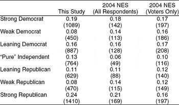
Note: Cell entries are column proportions with counts underneath in parentheses. Table omits National Election Study (NES) respondents who express identification with minor parties.
As shown in Table 2, a notable difference between the NES sample and the one used here is the level of political information. Almost all respondents in this study were able to identify the party in control of the House and Senate, whereas NES respondents were significantly less likely to know these answers. It should be noted that question wordings and survey mode were different for these surveys. Most important, the NES questions on congressional party control asked respondents who controlled each chamber beforethe most recent election, whereas this survey (conducted after the 2004 election) asked respondents who currently control each chamber. Although somewhat speculative, it could be argued that the NES question is more challenging and would be likely to produce more incorrect and “don't know” responses than the one used here. Furthermore, the impact of survey mode, specifically whether interviews are conducted in person or over the Internet, may be expected to affect responses, in particular whether respondents who are not certain about their answer are willing to guess or will be likely to give “don't know” responses. Because the analyses presented here use political information as an independent variable, this lack of representativeness is less of a problem. It will be important, however, for readers to keep in mind that the sample is more informed than the voter population as a whole.Footnote 9
Sample Knowledge of House and Senate Party Control
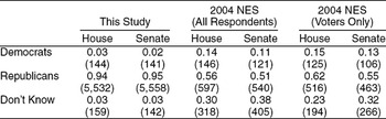
Note: Cell entries are column proportions with counts underneath in parentheses. Question wordings are different between National Election Survey (NES) and the survey used in this article.
For this survey, a list of 31 significant and important Senate votes was compiled by examining all roll calls during 2004 and 2005. These votes were chosen because of their relation to significant political issues that citizens would likely care about. Consideration was also given to the ease with which information about the vote could be summarized on a questionnaire and communicated to respondents. For this reason, important votes on things such as complex appropriations bills were left off the survey. The chosen votes—on 21 amendments and 10 bills—were selected from a variety of issue areas such as national security, the environment, lawsuit reform, and tax rates. A list of the votes used is found in Table 3, along with Senate yea and nay totals for each vote and the distribution of respondent answers on the corresponding survey questions. Full question wordings for all survey items used in this study are found in Appendix A.
List of Senate Votes Used in Survey

Note: Asterisks on Senate vote totals denote measures for which only cloture votes (and not passage votes) are available. For these votes, separate bill parameters are estimated for the cloture vote and for citizens’ responses to survey questions. Due to rounding, respondent vote percentages may not add to one hundred. γj and αj are question parameters as described in Equations (1) and (2). For measures with only Senate cloture votes, the estimated parameters for citizen survey responses, rather than those for Senate cloture votes, are presented.
Each respondent in the survey was given a random sample of 15 of the 31 Senate vote descriptions. For each bill or amendment selected, the respondent was given a bullet point description of the proposal and its key components, and then was asked how he would vote—“yes”, “no” or “don't know” (see Figure 3 for an example of a question as seen by respondents). Although different from traditional survey measures of citizens’ policy views, this question format provides a basis for directly comparing the positions of voters and candidates on the same scale. These longer items can more easily be presented to respondents in the Internet survey mode than would be possible with other verbal (in person or over the phone) methods.
Example of Question Format

Polling respondents on specific issue positions provides several advantages over simply asking people to quantify their overall ideology. First, these items are more concrete and hence more likely to be perceived in the same way. This is in contrast to ordinal scales, whose values have no objective definition. Second, polling on actual Senate proposals will allow for the direct comparison of voter ideal points and legislator positions, which is not generally possible with ordinal ideological scales. Finally, by polling respondents on many proposals across a wide range of issue areas, we are making no a priori assumptions about the policy dimension that structures their political beliefs. As discussed, we essentially allow respondents, through their answers, to tell us how different issues and proposals relate to the primary dimension of policy ideology (if there in fact is one) that is guiding their vote choices.
In addition to measuring policy views, the survey contains a series of political information items. I construct a measure of political information by asking each respondent nine questions about general political matters such as whether taxes have gone down or up since the year 2000, who controls each of the two branches of Congress, and who pays the majority of funds used to run public schools—the federal government or state and local governments. These questions are designed to measure people's understanding of and attention to the political landscape.
Estimating Policy Views and Political Information
To obtain estimates of the ideology of respondents regarding federal policy, I employ the technique of ideal point estimation. Under this framework, actors (in this case, citizens, senators, and the president) are each assumed to have some underlying level of policy ideology. Their answers to questions or their decisions on roll call votes are generated stochastically from these underlying levels of ideology based on the character of the bill or question under consideration. Here, I follow the general approach of Clinton, Jackman, and Rivers (Reference Clinton, Jackman and Rivers2004) in assuming quadratic utility functions for all actors and errors that follow the normal distribution. Footnote 10 In its basic form, this setup implies a probit link ideal point model under which the probability of a ‘yea’ vote by actor i on proposal j is P(yij = 1 | γ, α, x) = Φ (γjxi − αj). In this model, χi represents respondent i's ideal point. αj and γj are vote-specific “difficulty” and “discrimination” parameters, which are related to how much support there is for a measure and how strongly the probability of voting for the proposal is related to the actor's ideological position. Preliminary analyses of the stated positions of both respondents and senators revealed a dominant first dimension, with further dimensions contributing little explanatory power.Footnote 11 Therefore, the analysis presented here focuses on a one-dimensional model of respondent and senator ideology.
The roll call voting data set used here consists of two different partitions. First, we have the roll call records of all Senate votes from January 1, 2004 through February 16, 2006, including President Bush's stated positions for all measures on which he publicly took a stand.Footnote 12 Second, we have survey respondents’ views on 31 significant roll calls during this time period. Because these questions were written to simulate as closely as possible the process of roll call voting on these same bills and amendments, we can assume that the positions of the two alternatives that respondents are choosing between are the same as the ‘yea’ and ‘nay’ positions on the Senate roll call vote that corresponds with the survey question.Footnote 13 It immediately follows, then, that the bill parameters γj and αj in the ideal point model are the same for a respondent answering a question as for a senator voting on the corresponding proposal. By imposing these restrictions in the estimation procedure, we are able to estimate ideal points for survey respondents and senators on the same scale, thus bridging the comparability gap that has, up until this point, prevented direct tests of the spatial voting mode.
The standard ideal point setup as described previously implies that for any two actors with the same ideal point xi, the probability of a ‘yea’ vote on a given proposal will be the same. This may be a sensible assumption when all actors in a model are legislators. Our roll call data set, however, contains senators, the president, and ordinary citizens. It seems likely that senators might vote more precisely than respondents with the same ideological positions. This could occur for a variety of reasons, including the fact that senators and the president are in many ways “professional position takers” and thus would be more experienced at mapping their ideological preferences into specific policy proposals. Furthermore, these actors typically have far more information about the specific proposals before them than do respondents. For these reasons, we need to take into account the possibility that the variance of senators’ voting error distributions may be smaller than those of respondents.Footnote 14 If the voting error variances for respondents are different from those for senators and the president, models that ignore this possibility will tend to produce biased estimates of these ideal points. Specifically, if respondents’ error variances are larger than those for senators and the president, a model ignoring this possibility will tend to estimate respondent ideal points as being more moderate than they actually are relative to those of senators and the president. Similar problems can also result when some classes of respondents have larger voting error variances than others. In particular, we may suspect that respondents with higher levels of political information would have smaller error variances in their position taking on specific policy proposals.Footnote 15
To address these issues, I employ a modified ideal point model in which the variance of senators’ error distributions is fixed at one (as in the standard setup), but respondents’ error variances are estimated based on their level of political information. This gives the equation P(yij = 1| γ, α, x, ϕ) = Φ [ϕi(γjxi − αj)] for respondents, where ϕi is a multiplicative factor that indicates how precisely respondent i votes. Higher values of ϕi indicate that the distribution of voting errors for respondent i has a smaller variance, whereas smaller values of ϕi mean that respondent i is more likely to make voting mistakes, discriminating less precisely based on her own ideal point and the characteristics of the proposals with which she is faced. Formally, I assume that ϕi is equal to one for both senators and the president, and allow the value of ϕi for respondents to be parametrized by their level of political information, with ϕi = exp(δ0 + δ1PolInfo i. This is equivalent to parametrizing the variance of respondent error variances as 1/ϕi = 1/exp(δ0 + δ1PolInfo i.Footnote 16 This heteroskedastic ideal point model allows for the likely possibility that ordinary citizens will state their policy positions with more error than do senators or the president.
In addition to measuring policy ideology, I also use an item response model to estimate each respondent's level of political information. Our task is similar here to measuring policy ideology. To begin, I assume that political information is a latent trait with different values held by each person. An individual with higher levels of political information will be more likely to give correct responses to our questions about the political and policy system. As it happens, this setup yields a latent traits model for political information that is of the same form as the ideal point model used to measure policy ideology. The model is well suited to this task because an equivalent specification is commonly used in educational testing and psychometrics (see Baker Reference Baker1992).
We now have the basic tools to measure the quantities of inference for our study—the policy views of citizens and the policy positions taken by senators and the president (all of which are directly comparable on the same scale) as well as the political information level of each respondent. We also have survey measures of respondents’ party identification and of their vote choice in the 2004 presidential election. The following section discusses the task of building a full model of citizen vote choice in order to investigate whether citizens’ voting decisions in real world elections are consistent with the assumptions of spatial voting theory.
DIRECTLY TESTING THE SPATIAL VOTING MODEL
Now that we have established the basic tools and background necessary for testing spatial voting in the 2004 presidential election, I move on to formally specify a complete statistical model of citizens’ voting decisions. In this model, the probability of voting for Bush (versus Kerry) is a function of a respondent's ideological location, level of political information, and party identification. I estimate respondents’ probabilities of voting for Bush as a probit regression model, including terms for respondent ideal point, political information and an interaction between the two.Footnote 17
Formally, I construct a Bayesian statistical model estimating the effects of ideology, party identification, and political information on respondents’ vote choices in the 2004 presidential election. For simplicity, I analyze only the two-party vote, coding respondent votes as 1 if they voted for George W. Bush and 0 if they voted for John Kerry. Votes for other candidates as well as abstentions are coded as missing values. The model I propose for presidential vote choice has four parts: ideal point estimation for senators (most notably John Kerry) and President Bush, ideal point estimation for survey respondents, political information estimation for respondents, and, finally, the estimation of a probit regression equation predicting respondents’ presidential vote choice as a function of ideal point and political information. These levels are estimated simultaneously in a single Bayesian statistical model.Footnote 18
The Statistical Model
The formal statistical model can be separated into four stages. The first stage of the model is the estimation of the ideal points of senators as well as President Bush in his public “voting” on Senate proposals. This section of the model uses the voting records of all senators and the president on all roll calls from January 2004 to February 2006. As discussed previously, this Senator Roll Call Equation fits a probit link ideal point model where, for each senator s on each roll call j

Because we have respondent's stated views on actual proposals that have been voted on in the Senate (and thus are included in the Senator Roll Call Equation (1)), I employ the same general framework to estimate respondents’ ideal points in the same policy space as senators and the president. To do this, I simply restrict the parameters for a given policy question to be identical to the bill parameters for the corresponding roll call vote taken by senators, allowing for the simultaneous estimation of ideal points of citizens and senators on the same scale.Footnote 19 The only difference between the ideal point model for senators and respondents is the inclusion of a multiplicative term to account for possible differences in voting error variances, as described previously.Footnote 20 This allows for the possibility that respondents and senators with identical ideal points may have different probabilities of choosing the alternative farthest from their ideal point on a given roll call. In other words, senators may vote more precisely, with less error, than respondents when faced with the same policy choices. The Respondent Roll Call Equation for the ideal points of survey respondents, indexed by i, is
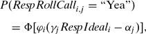
where γj and αj are bill parameters for the corresponding Senate votes in Equation (1). I then allow ϕi to vary based on respondents’ level of political information, as discussed previously, with

In the next stage of the model, I employ an item response framework, as used in psychometrics and educational testing, to estimate respondents’ political information levels based on their responses to questions about politics and the political system. The form of this model is equivalent to that of the basic ideal point model, but instead of measuring people's positions on a liberal-conservative policy ideology, it is used to estimate their level of political information. For each respondent i and each question k from the survey's political information battery, we have the Political Information Equation

where qi,k = 1 if respondent i gives a correct answer to question k, and equals zero otherwise.Footnote 21 λk and ωk are parameters estimating the difficulty and discrimination of question k at tapping political information.
The final section of the model is a probit regression predicting respondents’ 2004 presidential vote using their policy ideology, political information, and an interaction between the two. Footnote 22 Furthermore, to account for possible differences in the way Democrats, Republicans, and independents may vote conditional on their policy views and information levels, separate regression coefficients are estimated for each of the three party identification groupings. The coefficient estimates from this level of the model will allow us to make inferences about the effects of party identification, policy ideology, and political information on vote choice. Formally, for respondent i, the probability of casting a vote for George W. Bush is given in the Presidential Vote Equation:
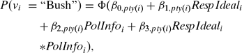
where pty(i) gives respondent i's party affiliation—Democrat, Republican, or independent. This amounts to estimating separate probit regression equations for Democratic, Republican, and independent respondents.
Party identification is measured using the standard NES question wording with seven possible responses from “Strong Democrat” to “Strong Republican.” For the purposes of the model presented here, leaners are treated as partisans, and independents consist solely of “pure” independents, yielding a three-category scale of Democrat, Republican, and independent. Alternate versions of the statistical model presented in this article have been run treating each of the seven party identification categories separately, and the substantive results of these models are similar to the three-category model presented later in the article. Therefore, I present the results of the more parsimonious model here.
Model Estimation: A Bayesian Approach
I estimate the model using a Gibbs sampler employed in the freely available software WinBUGS (Spiegelhalter, Thomas, and Best, Reference Spiegelhalter, Thomas and Best1999). This estimation method simulates draws from the posterior distribution over the model's parameters by iteratively sampling from the conditional posterior distributions of each parameter given the current simulated values of all other parameters (for an accessible social science introduction to Bayesian analysis including Gibbs sampling, see Jackman Reference Jackman2004). The model is estimated in an unidentified state, and the results are postprocessed to enforce the restrictions that the respondent ideology and information estimates each have mean zero and variance one and that these scales are oriented such that higher values represent more conservative ideologies and higher levels of information, respectively. The result of this estimation procedure is a series of random draws from the posterior distribution over the model's parameters. These simulated draws are then used to obtain estimates of the value of different variables and to conduct hypothesis tests and make other inferences. Although the algorithm appeared to reach convergence fairly rapidly, a conservative strategy was still used, running two independent sampling chains, each for 500,000 iterations. The first 100,000 iterations of each chain were dropped as a burn-in period, and the chains were thinned to save every 10th iteration. In total, this yielded 40,000 samples from the posterior distribution over the model's parameters on which we can base our inferences.
RESULTS
The ultimate goal of estimating this model of citizen voting is to directly test whether various types of citizens employ spatial voting rules when making choices in actual elections. Before looking at the results of these tests, however, we can examine the estimated bill parameters for the Senate roll calls on which respondents also stated their preferences. Table 3 lists the estimates for γj and αj, seen in Equations 1 and 2, often referred to as “discrimination” and “difficulty” parameters, respectively. Loosely speaking, γj describes how strongly and in what direction an actor's ideal point is related to his probability of voting for a proposal, and αj is related to the overall level of support for a proposal. By focusing on the estimates of γj for each of the proposals shown, we can get a sense for which issues provide the most structure to the underlying ideological dimension on which we estimate the positions of respondents, senators, and the president. Actors’ votes on proposals with larger discrimination parameters (in absolute terms) will provide more influence on their ideal point estimates, whereas votes on proposals with discrimination parameters near zero will have little effect on these estimates. As seen in Table 3, the discrimination parameters for the 31 proposals shown to respondents have a wide range of values. Some, such as the Patriot Act reauthorization, increasing the federal minimum wage, gay marriage, and environmental issues have a large impact on ideal point estimates. Others, such as overtime pay regulations and military base closure delays, have little or no impact. Overall, the results demonstrate that a wide range of issues contribute to the policy ideology of respondents and senators. Furthermore, these estimates correspond well with conventional notions of ideology in the American politics. Proposals that would move policy in what most observers of American politics would call the liberal direction tend to have negative values of γj, and conservative proposals have positive ones. These results provide validation for the measure, suggesting that the ideal point estimates for respondents, senators, and the president correspond well with general intuition.
We can also examine the ideal points for both senators and respondents as estimated in the full model. The densities of these estimates as shown in Figure 4 for senators and respondents, separated by partisanship. We see clearly that, as expected, Democratic respondents tend to have more liberal ideal points, whereas Republicans are generally more conservative. Independents are on average closer to the middle. One notable feature of Figure 4 is the number of respondents whose estimated ideal points fall to the left of Kerry or to the right of Bush or even to the left or right of the estimated positions of all senators. In a sense, such results should not be unexpected if one assumes that elected representatives come from near the median of their constituencies. Especially in the large and relatively heterogeneous constituencies of the Senate (as opposed to the House), we may expect some nontrivial fraction of citizens to hold ideologies to the outside of all senator ideal points. Many public opinion scholars, however, may object to the notion that a significant portion of the electorate could hold ideologies that are so extreme.
Estimated Senator and Respondent Ideal Point Densities

There are several important issues to bear in mind when interpreting these results. First, it should be noted that although senator ideal points are estimated relatively precisely, each respondent states his or her position on a maximum of 15 policy proposals, which means that the ideal point of each individual is estimated with a considerable amount of uncertainty. This is likely to make the overall distribution estimated citizen ideal points appear more spread out. Furthermore, respondents who take positions consistently on the liberal or on the conservative side of all policy proposals will be estimated to have very extreme ideal points.Footnote 23 In fact, more than 4% of respondents in this study expressed such consistently liberal or conservative opinions across all proposals they were shown.
It should also be pointed out that, as mentioned previously, the sample used in this study is not designed to be strictly representative at the national level. Therefore, these plots are not presented as definitive estimates of the distribution of ideology among Americans generally, but rather are shown in order to illustrate how citizen ideology in this sample has been scaled alongside the positions of senators and the president. Breaking these distributions down by respondents’ level of political information reveals that as information levels increase, partisans tend to become more ideologically extreme. Because this sample overrepresents those with high levels of political information, it is likely that it correspondingly overrepresents citizens with both extremely liberal and extremely conservative ideologies. This would be problematic if the task of this study was to estimate characteristics of the national distribution of ideology, but because the focus here is on the relationships between ideology and vote choice, and both ideology and information level are included in the model as predictors, this is not a serious issue.
Finally, and perhaps most important, the roll call voting models for senators and respondents differ importantly in terms of their error variances as seen by the addition of the parameter ϕi. Because of this, a respondent and senator with similar ideal points will have different probabilities of supporting a given proposal. For example, a respondent who has the same ideal point as John Kerry will have a higher probability than Kerry does of voting on the conservative side of a given roll call. This is because respondents (especially those with lower information levels) tend to vote less precisely than senators. This means that respondents estimated to have ideologies more liberal (conservative) than most senators would not necessarily be predicted to have produce a more extreme roll call voting record in terms of the proportion of votes cast in the liberal (conservative) direction. Estimating an ideal point model that ignores these differences in voting error between respondents and senators produces respondent ideology estimates that are less spread out relative to those for senators. It is important then to interpret the relative positions of respondents and senators in light of these differences. As mentioned previously, the overall substantive results from the full model have been verified using simpler stepwise models in which both ideal points and information levels are estimated using standard (homoskedastic) ideal point models, and these point estimates are used as independent variables in probit regressions predicting presidential vote choice.
An important question raised by these basic results is whether it is a reasonable assumption that ordinary voters, especially those at lower levels of political information, have developed preferences on the same ideological dimension on which political elites make policy decisions. Recent work such as Ansolabehere, Rodden, and Snyder (Reference Ansolabehere, Rodden and Snyder2008) suggests that ordinary Americans do in fact possess meaningful ideologies related to the (arguably symbolic) issues presented on surveys such as the NES. The approach used in this study, however, offers the much stronger finding that citizens hold ideologies on matters of specific government policies such as those debated in the U.S. Congress and, even further, that these ideologies are structured similarly to those of legislators and the president.
To test the robustness of this finding, I separately estimate ideal point models for various subgroups of respondents and compare these to the estimates from pooled ideal point models estimated from all respondents, senators, and the president (see Appendix B for a fuller discussion of these analyses). If the ideologies of citizens are structured differently from those of political elites, we would expect the results obtained from an ideal point model estimated for citizens, senators, and the president together would be different from those estimated only for respondents. I find, however, that respondent ideal points estimated from data on respondents, senators, and the president together are nearly identical to those estimated separately for respondents and senators. This is also the case when comparing ideal points estimated for all respondents together with those estimated separately for low, medium, and high information respondents. For example, ideal points estimated separately for respondents who correctly identified the Republicans as having a majority in the House and those who did not are correlated at well above 0.9 with ideal points estimated for all respondents pooled together. These results suggest that not only do ordinary citizen possess real ideological beliefs, but also these beliefs map onto specific policy proposals in much the same way as do the ideologies of senators and the president. Furthermore, these ideological structures are similar across most classes of respondents, including those of lower levels of political information.
Model Estimates
Table 4 presents the three sets of coefficients estimated in the Presidential Vote Equation (5) of the model, along with the parameters estimating the relative amounts of voting error variance for respondents of different information levels and the estimated ideological positions of Bush, Kerry, and the midpoint between the two candidates. Because each probits coefficient is indexed by respondent party identification, we can think of this as three separate probit regression equations—one for Democrats, one for independents, and one for Republicans.Footnote 24 The first thing to notice is that, consistent with the first requirement for spatial voting, the coefficients on respondent ideal point are all positive and substantively large with probability well more than 95% for each party identification grouping. This implies that policy views have have a sizable effect on voting behavior even when holding party identification constant. It is not the case that people's behavior is simply a knee-jerk reaction to the “affective orientation” they have toward the two parties. Those who tend to hold more liberal policy positions are more likely to vote for Kerry, and those whose policy positions are more conservative are more likely to support Bush, independent of their party identification. This effect is also substantively quite large for each party identification grouping. For respondents with average levels of political information, a shift of one standard deviation in a respondent's ideology will produce a shift of 3.42, 29.90, or 2.57 on the probit scale for Democrats, independents, and Republicans, respectively. Furthermore, we see that the coefficient on RespIdeal for independents is significantly larger than those for Democrats and Republicans. In fact, the main effect of policy ideology is predicted to be largest for independents with probability well above 95%. This indicates that, controlling for level of political information, independents seem to be more influenced by policy views than are partisans.Footnote 25
List of Senate Votes Used in Survey

Note: Model estimates are shown with 95% highest posterior density regions underneath in parentheses. The mean and standard deviation of respondent ideology and information are zero and one, respectively, with higher values of ideology representing more conservative views and higher values of information representing more informed respondents.
We also see that the estimated coefficients for for the interaction between policy ideal point and political information are all positive. Although the highest posterior density regions for these parameters for Republicans and independents include zero, the posterior probability that these coefficients are positive are all at or very near 95%. Although the results for independents and Republicans are somewhat ambiguous, they do show that higher information levels clearly result in a stronger reliance on policy views in presidential voting for Democratic respondents. Taken together, this evidence provides support for the idea that information moderates the use of spatial decision making in voting behavior. Although this evidence is not completely conclusive, it differs from the finding of Ansolabehere, Rodden, and Snyder (Reference Ansolabehere, Rodden and Snyder2008) that information has no meaningful effect on the role of policy views in voting behavior.
In addition to looking at the coefficient estimates, inspection of the model's predicted probabilities is another (perhaps more intuitive) way to understand the model's implications. Figure 5 shows the predicted probabilities from the Presidential Vote Equation (5) for people with low, medium, and high levels of political information, defined as the 0.05, 0.5 and 0.95 quantiles of the sample distribution for political information (PolInfoi). The most obvious feature of these plots is the convergence of the behavior of partisans as political information increases. Although significant gaps remain between the response probabilities of Republicans, Democrats, and independents of similar policy views even at the highest levels of political information, we clearly see that the large effect of party identification for low information respondents is dampened as citizens become more aware and informed about the political environment. The voting behavior of partisans, specifically their use of ideology in their voting decisions, differs sharply across information levels. Although independents also show differences by information level, such differences are much smaller than those observed for partisans.
Differences in Party Identification Effects by Political Information Level

Referring back to the typology developed in Figure 2, we see that low information partisans behave largely in accordance with the predictions of the simplified “Michigan model” under which partisanship is the primary determinant of vote choice and ideology has little or no effect. Independents, in contrast, show strong relationships between ideology and vote choice even at lower information levels. The behavior of medium and high information respondents most closely resembles the hybrid model under which both ideology and party identification have their own effects on vote choice. As information levels increase, we see that partisans converge toward the behavior of independents, reducing the main effect of party identification. However, even for respondents at the highest information levels (of what is a highly informed sample), large gaps remain between the behavior of Democratic, independent, and Republican respondents.
Table 4 also presents estimates of δ0 and δ1, which describe how respondent information levels are related to the variance of their roll call voting error distributions. These estimates indicate that, as expected, senators and the president exhibit less error than do ordinary citizens in their roll call voting. Furthermore, respondents with higher levels of political information tend to have smaller voting error variances than those with less information (recall from Equation 3 that ϕi = exp(δ0 + δ1PolInfo i, where 1/ϕi gives respondent i's voting error variance). These estimates imply that respondents of average information levels have error variances that are approximately 23% larger than those for senators and the president, whose error variances have all been fixed at one.Footnote 26 High information respondents, defined as those at the 0.95 quantile of sample information, are estimated to have error variances 19% larger than those of senators and the president, whereas low information respondents, defined as those at the 0.05 sample quantile of information, show error variances that are 30% larger. Therefore, respondents on the whole show more propensity for error in their roll call voting than do senators and the president, as would be expected given their relative inexperience in such position taking. We also see important differences between respondents, with more informed citizens showing smaller error variances. Because we account for this error rather than ignore it, our ideal point estimates are not adversely affected by this heteroskedasticity.
Assessing Bias in Spatial Voting
We have already seen from the model's predicted probability plots that although respondents of all political stripes rely heavily on their ideological positions in making voting decisions, there is wide divergence between the voting rules used by Democrats, Republicans, and independents at virtually all levels of political information. This section moves on to directly test the second condition of unbiased spatial voting, namely, that respondents should be equally likely to vote for either candidate when their ideal point falls at the midpoint between the two candidates’ positions. Combined with the first condition, this implies that citizens with ideologies to the left of the midpoint between Bush and Kerry will be most likely to vote for Kerry, citizens to the right of the midpoint will probably vote for Bush, and those whose views fall at the midpoint between the candidates will be indifferent between the two candidates.
We can now use the estimated parameters of the Presidential Vote Equation (5) to solve for the implied indifference point between Bush and Kerry for a voter with a given party identification and political information level. To do this, we simply find the value of respondent ideology that causes the Presidential Vote Equation (5) to equal one half, implying a 50% chance of voting for Bush and a 50% chance of voting for Kerry. This will take place when the normal cdf is evaluated at zero. Therefore, the implied indifference point for a respondent i with a given level of political information who identifies with party pty(i) is calculated as
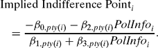
Figure 6 plots the implied indifference points along with 95% credible intervals for respondents of each category of party identification, varying by political information level. As we saw previously in the predicted probability plots, the divergence between Democrats and Republicans, even those at similar political information levels, is stark. Again, independents’ behavior falls somewhere in between with partisans converging in behavior toward independents as their political information increases. Even at the highest information levels, the differences in the implied indifference points of Democrats, independents, and Republicans show large differences. We can say with virtual certainty across most levels of political information that the implied indifference points for Democrats are greater than those for independents and that those for independents are greater than those for Republicans.
Implied Indifference Points Used by Voters Under Spatial Voting

The question now becomes what indifference point would be employed by voters using an unbiased spatial voting rule. To answer this question, we refer back to the Senator Roll Call Equation (1) of the statistical model. Using Kerry's Senate votes and Bush's publicly stated positions on Senate proposals, the model estimates the ideal points of Bush and Kerry at points θ and φ , respectively, both estimated on the same scale as our survey respondents’ policy views. To obtain an estimate of the true midpoint between Bush and Kerry's policy positions, we simply take the midpoint between the estimated ideal points of Bush and Kerry, which can be calculated as (θ + φ)/2. Under unbiased spatial voting, this would also be the indifference point for voters. From the Senator Roll Call Equation (1) of the model, we obtain an estimate of the midpoint between Bush and Kerry's ideal point of 0.23 with a 95% credible interval of (0.04, 0.42), as shown in Table 4.
Using the formula from Equation (6), we see that the model predicts the implied indifference point for highly informed independents at 0.17, with a 95% credible interval of (0.08, 0.26). This value is quite close to the 0.23 estimated for the midpoint between Bush and Kerry's positions, and suggests that highly informed independents are acting largely in accordance with the predictions of spatial voting, showing little or no spatial bias in their vote decisions. The estimated implied indifference point values for Republicans and Democrats are considerably farther away from our estimate of the true midpoint between Bush and Kerry's ideal points. Furthermore, the estimated values for lower information partisans are markedly different. As an illustration, note that even a highly informed Democrat would have to have an ideal point of 0.53, which is more than twice as close to Bush as to Kerry, in order to be indifferent between the two candidates. High information Republicans would have to have an ideal point of −0.43, which is almost as liberal as Kerry's estimated position, in order to have a 50% chance of voting for Kerry. The corresponding numbers for average and low information partisans are even more stark. In fact, the model predicts that Democrats at lower levels of political information would actually have to be more conservative than Bush in order to have a greater than 50% chance of voting for him. Republicans of even average levels of information or lower must be more liberal than Kerry in order to be indifferent between the two candidates. In contrast, independents, even those with lower levels of political information, seem on average to be engaging in unbiased or nearly unbiased spatial voting. In fact, low information independents fare at least as well or better than even the most informed partisans by the standards of unbiased spatial voting.
DISCUSSION
Building on the simple premise that citizens tend to vote for the candidate whose position is closest to their own, spatial voting theory has generated a widely applicable set of predictions and insights that have relevance for nearly all areas of political science. Direct examination of the foundations of the spatial approach, however, has until now been largely impossible. This article provides what is the most direct test to date of the central axioms underlying the spatial theory of voting—that increasing conservatism should be related to higher probabilities of voting for the more conservative candidate and that the point at which voters are indifferent between the two candidates should fall at the actual midpoint between the candidates’ positions.
By measuring citizen ideology on the same scale as the position of candidates, we are able to directly uncover the relationships between voters’ ideological proximity to Bush and Kerry and their vote probabilities in 2004 presidential election. First, this new approach has demonstrated that not only do ordinary citizens possess real ideological beliefs, but these preferences are meaningfully related to the ideological dimension on which actual federal policies are debated in Congress and structured in a similar way to the ideologies of senators and the president. Furthermore, the results presented here demonstrate that although the vast majority voters employ ideological considerations in making their vote choices, there are important differences in terms of which voters can be said to follow the assumptions of unbiased spatial voting. In particular, voters who do not identify with either of the major political parties approximate this spatial ideal extremely well. Even at lower levels of political information, the behavior of independents is very close to what would be predicted by unbiased spatial voting. Furthermore, the voting decisions of more informed independents are statistically indistinguishable from completely unbiased spatial voting rules. Although the voting decisions of partisans are related to their ideological positions, their decision rules are significantly different from what would be implied by purely spatial voting. At lower levels of political information, partisans show large amounts of spatial bias toward the candidate of their party. As information levels rise, these biases are decreased and the behavior of both Democrats and Republicans converges toward that of independents. Even at high information levels, however, partisans diverge much more sharply from the implications of spatial voting theory than do independents.
Although these findings resolve a considerable amount of ambiguity regarding the use of spatial voting by ordinary citizens in real world elections, they also suggest several new avenues for future research. This article identifies the use of spatial decision making by estimating the precise relationships between voters’ ideological locations and the actual positions taken by candidates. Future research should go deeper to examine the possible mechanisms that could be producing these relationships. For example, it is possible that partisan projection accounts for the observed differences in the use of spatial voting, with voters making unbiased spatial decisions based on their perceived proximity to the candidates rather than the true distances. It would also be important to examine how these results are affected when moving from the relatively high information world of presidential elections to other contests such as House or Senate races. Finally, it bears noting that the degree to which citizens employ spatial voting rules could vary across election years. For example, 2004 is considered by many to have been a highly partisan election. It was also a relatively close election, with factors such as the economy not favoring either party dramatically. Analyses of future elections following the general framework used in this article could determine whether the results presented here, both in terms of the strength of ideology's influence on voting decisions and the level of spatial bias in citizens’ decision rules, apply equally well to different political climates and electoral circumstances.
The most important finding of this paper is that a significant fraction of the electorate casts their ballots largely in accordance with the assumptions of spatial voting theory. Although partisans of virtually all political information levels deviate systematically from these predictions, policy views are still found to have significant effects on their voting decisions across all but the lowest levels of political information. Overall, voter behavior corresponds closely with the assumptions of formal models in which citizens’ ideological proximity to candidates and party attachments combine to determine the utility they receive from voting for each candidate. These results highlight the strengths of the spatial voting model, demonstrating that although voting decisions are the product of many different influences, much of citizen behavior in high-profile elections can be captured by a relatively simplified and parsimonious theoretical framework.
APPENDIX A: SURVEY QUESTION WORDINGS
Party Identification Questions (Standard NES Wording)
Generally speaking, do you usually think of yourself as a Republican, a Democrat, or an independent?
For partisans: Would you call yourself a strong [Democrat/Republican] or a not very strong [Democrat/Republican]?
For independents: Do you think of yourself as closer to the Democratic or Republican Party?
Senate Proposal Questions
As you know, your representatives and senators in Washington vote on issues that affect our country. On the following pages, we ask you about some actual proposals before the U.S. Senate. We give you a brief description of each proposal. Tell us whether you would support each proposal and how you think your senators would vote when these issues come up. If you aren't sure how one or both of your senators would vote, try to guess how they would vote when faced with this proposal based on what you know about them.
S 397: Protection of Lawful Commerce in Arms Act
• Prevents people from suing gun manufacturers and dealers for the misuse of their products, including when crimes are committed with guns they make or sell.
• The bill would still allow lawsuits for product defects and malfunctions.
• Requires safety locks for all guns sold or transferred.
• Increases penalties for possession or use of “armor-piercing” ammunition when committing a crime.
S 1307: Central American Free Trade Agreement
• Promotes free trade between the United States and Central American countries.
• Reduces tariffs, duties, and other fees and taxes on imports and exports between the United States and Central American countries for items such as textiles and agricultural goods.
S AMDT 826 to HR 6: Greenhouse Gas Reduction and Credit Trading System
• Would require that industries reduce their production of greenhouse gasses to year 2000 levels within five years.
• Would establish a credit trading system that would allow companies who are unable to reduce emissions to this level to buy credits from other companies who reduce their pollution to farther below the limit.
S AMDT 44 to S 256: Minimum Wage Increase
• Would raise the minimum wage to $5.85 immediately, then to $6.55 after one year, and to $7.25 in two years.
• The minimum wage before this bill was proposed was $5.15.
HR 1997: Unborn Victims of Violence Act
• Makes it an additional crime to harm or kill a fetus while committing a violent crime against a pregnant woman.
• Does not require that the attacker knew the woman was pregnant.
• Does not apply to abortions.
S AMDT 3183 to S 2400: Hate Crimes Amendment
• Would classify crimes motivated by a victim's race, color, religion, sexual orientation, disability, or national origin as “hate crimes” to be prosecuted in federal (not state) courts.
• Authorizes $5 million per year over the next two years for the Justice Department to assist state and local authorities in investigating and prosecuting hate crimes.
S AMDT 1085 to HR 2419: Remove Funding for “Bunker Buster” Warhead
• The “bunker buster” is a small nuclear warhead designed to destroy fortified underground positions by breaking through rock or concrete to a certain depth before exploding.
• This amendment would stop the use of federal funds for the development of the proposed “bunker buster” nuclear warhead.
• The money would instead be used to pay down the national debt.
S AMDT 367 to HR 1268: Remove Funding for Guantamo Bay Detention Center
• Eliminates $36 million in funding, which was planned to build a new permanent prison facility at Guantanamo Bay, Cuba, to house detainees from the war on terrorism.
S AMDT 1626 to S 397: Child Safety Locks Amendment
• Requires gun manufacturers and sellers to include child safety locks on all firearms sold or transferred.
S 256: Bankruptcy Abuse Prevention and Consumer Protection Act
• In Chapter 7 bankruptcy, a debtor sells off most of his or her property and pays as much of his or her debts as he or she can, and the rest of his or her debts are erased. In Chapter 13 bankruptcy, debtors work out a payment plan to pay off all or most of their debts.
• This bill would force debtors into Chapter 13 bankruptcy in which they must pay off their debts (rather than have them erased) if they are able to do so while still earning above their state's median income.
• Places child support and alimony payments into the category of nondischargeable debts, which must still be repaid under all forms of bankruptcy.
• Allows some special treatment for active-duty military members, veterans, and those with serious medical conditions.
• Requires debtors to pay for and attend credit counseling before filing for bankruptcy.
• Requires that monthly credit card statements include warnings and explanations about interest rates and fees.
• Caps home equity protection at $125,000 if debtor purchased the home within 40 months of filing for bankruptcy.
S 5: Class Action Fairness Act
• Class action lawsuits are brought in the name of a group of people who all claim to have been affected similarly by a product, procedure, or other act. These lawsuits try to get companies who allegedly caused this harm to pay the group that was affected.
• This bill requires that all class action settlement proposals include estimates of lawyers’ fees if payment for the court's ruling are in the form of coupons.
• Requires that all members of the affected class be notified about settlement proposals.
• Sends to federal (not state) court all civil action in which the case involves more than $5 million, concerns a plaintiff of one state and a defendant of another, or involves a foreign state or its citizens.
• Grants judges expanded powers to determine whether class action settlements are fair, reasonable, and adequate.
S AMDT 2807 to S CON RES 95: Reverse Tax Cuts on High Incomes
• Rolls back tax cuts for those whose income is above $1 million per year.
• Uses the funds raised for increases in homeland security spending and for paying down the national debt.
S AMDT 168 to S CON RES 18: Prohibit Drilling in ANWR
• Would keep the Arctic National Wildlife Refuge (ANWR) in Alaska closed to oil drilling.
S AMDT 1615 to S 397: Broaden Definition of Armor-Piercing Ammunition
• Would classify any handgun ammunition that is capable of penetrating body armor as “armor piercing.”
• Would ban all such “armor-piercing” handgun ammunition as well as rifle ammunition that is marketed or designed specifically for armor piercing.
S J RES 40: Federal Marriage Amendment
• Amends the Constitution of the United States to include a definition of marriage being only between a man and a woman.
• Prevents individual states from recognizing marital status or legal benefits from any other unions except those between a man and a woman.
S AMDT 2799 to S CON RES 95: Cigarette Tax Increase
• Increases taxes on cigarettes to $1 (the tax was previously 39 cents).
• Uses the funds raised by these taxes (estimated at $30.5 billion) to pay for increased spending on health programs such as medical research, disease control, wellness, tobacco addiction counseling, and preventative health efforts, including substance abuse and mental health services.
S AMDT 3107 to S 1637: Overtime Pay Regulations
• The Department of Labor has proposed regulations that would eliminate overtime pay for anyone making over $100,000 per year or anyone making between $23,660 and $100,000 per year who works as an administrator or in a professional “white-collar” job.
• This amendment would get rid of these regulations.
S AMDT 3379 to S 2400: Raise Tax Rate on Highest Income Bracket
• Raises the tax rate on all income above $326,450 per year from 35% to 36%.
• Uses the funds raised to pay for the security and stabilization of Iraq.
HR 4250: Jumpstart Our Business Strength Act
• Will reduce the corporate tax rate on domestic manufacturers and small corporations from 35% to 32% and provide about $145 billion in tax reductions to U.S. corporations over the next 10 years.
• Allows individual taxpayers who pay no state income tax to deduct their state sales tax on their federal tax returns.
• Would repeal certain tax regulations on foreign imports. The World Trade Organization (WTO) had ruled these taxes in violation of their regulations, so repealing them will stop the WTO from penalizing U.S. exports.
• Allows private collection agencies to track down citizens who have not fully paid their taxes.
• Eliminates certain tax shelters and tax avoidance practices for businesses. This is expected to bring in about $63 billion in new tax revenue over the next 10 years.
• Ends federal price supports for tobacco farmers and allots $10 billion to tobacco farmers as compensation.
• Allows the U.S. Food and Drug Administration to regulate tobacco products.
S 2061: Healthy Mothers and Healthy Babies Access to Care Act
• Places a limit of $250,000 on noneconomic (pain and suffering) damages in lawsuits against obstetricians, gynecologists, and nurse midwives for medical malpractice.
• Allows people to sue these types of doctors for malpractice only within three years of the date of the appearance of injury or one year after the claimant discovers the injury.
• Allows punitive damages (meant to punish the accused) only in cases where doctors intentionally or knowingly harmed patients.
• When punitive damages are allowed, they are limited to two times the economic damages or $250,000, whichever is greater.
• Limits the liability of manufacturers, distributors, and providers of gynecological products that have been approved by the U.S. Food and Drug Administration.
• Allows payments of certain medical malpractice verdicts to be paid in installments over time (rather than all at once).
S AMDT 2937 to HR 4: Child Care Funding for Welfare Recipients
• Provides an additional $6 billion to states over the next 5 years for child care for welfare recipients.
• This is paid for by renewing customs fees that would have expired.
S AMDT 3158 to S 2400: Military Base Closing Delays
• This measure would delay for two years the planned closing of several military bases in the United States.
• Would also limit some of the planned closing of overseas military bases.
S AMDT 3584 to HR 4567: Stopping Privatization of Federal Jobs
• Would stop the government from contracting out 1,100 jobs in the Homeland Security Department's Citizenship and Immigration Services bureau to private companies and would keep these jobs within the federal government.
HR 1308: Working Families Tax Relief Act
• Would extend the $1,000 per child tax credit through 2009.
• Would reduce taxes by extending the upper limit adjustment for the 10% tax bracket through 2010. This means that married couples would pay a 10% tax rate on their first $14,000 of yearly income. Without this extension, only the first $12,000 would be taxed at 10% and the rest at a higher rate.
• Would extend tax breaks for married couples (the elimination of the so-called “marriage penalty”) through 2008.
• Would extend the existing income tax exemption from the alternative minimum tax for couples with incomes below $58,000.
• Extends the Research and Development tax credit, which allows businesses to deduct 20% of qualified research expenses, through 2010.
S AMDT 1026 to HR 2161: Prohibiting Roads in Tongass National Forest
• Would prohibit federal funds from being used to plan or build new roads for the purpose of logging in the Tongass National Forest in Alaska.
S AMDT 902 to HR 6: Fuel Economy Standards
• Would require that passenger cars made before 2008 average 25 miles per gallon.
• This requirement would be gradually increased to 40 miles per gallon by the year 2016.
• Nonpassenger (or commercial) vehicles would have to average 16 miles per gallon before 2008, and this standard would gradually increase to 27.5 miles per gallon.
HR 3199: USA Patriot Act Improvement and Reauthorization Act of 2005
• The USA Patriot Act gives the federal government expanded powers of surveillance, investigation, and prosecution against suspected terrorists, their associates, and those suspected of financing terrorism.
• This bill would extend two of the Patriot Act's provisions for four more years. These provisions involve allowing the government to use roving wiretaps to listen in on phone conversations and other communications and permitting secret warrants for books, records, and other items from businesses, hospitals, and organizations such as libraries.
• The bill would permanently extend most of the other provisions in the Patriot Act, allowing the government to have broader powers of investigation over its citizens and others living within its borders.
S AMDT 278 to S 600: Family Planning Aid Policy
• Under current U.S. policy, government money cannot be given to family planning organizations in other countries if these organizations perform or promote abortions, even if the U.S. money is not specifically used for this purpose.
• This vote would reverse this policy and allow U.S. funds to go to family planning organizations in other countries regardless of whether they promote or perform abortions.
S J RES 20: Disapproval of Mercury Emissions Rule
• This vote would replace the current credit trading system for mercury emissions from power plants with a policy of strict limits on the amount of mercury that power plants can release into the atmosphere.
S AMDT 1977 to HR 2863: Banning Torture by U.S. Military Interrogators
• Would prohibit “cruel, inhuman or degrading treatment or punishment” against anyone in the custody of the U.S. military.
• Limits interrogation techniques to those authorized in the U.S. Army Field Manual on Intelligence Interrogation.
S AMDT 1645 to S 397: Increase Criminal Penalties for Armor-Piercing Ammunition
• Would increase penalties for the use or possession of armor-piercing ammunition while committing a crime.
• Would direct the Attorney General to conduct a study regarding such armor-piercing ammunition and report back to Congress.
Political Information Questions
Have federal income tax rates increased or decreased since 2000?
Increased
Stayed the same
Decreased
Don't know
Has the federal budget surplus increased or decreased since 2000?
Increased
Stayed the same
Decreased
Don't know
Who provides most of the money to run public schools in the United States?
Federal government
State and local governments
About equal
Don't know
When people are charged with a crime such as burglary, driving while intoxicated, or murder, what type of law are they usually charged with violating?
Federal law
State law
Don't know
Who favors raising the minimum wage?
Democrats
Republicans
Both
Neither
Don't know
Who favors developing a national missile defense shield?
Democrats
Republicans
Both
Neither
Don't know
Who favors putting fewer government restrictions on businesses? Liberals
Conservatives
Both
Neither
Don't know
Who currently controls the U.S. House of Representatives?
Democrats
Republicans
Don't know
Who currently controls the U.S. Senate?
Democrats
Republicans
Don't know
APPENDIX B: IDEAL POINT ANALYSIS
This appendix focuses on establishing the validity of the statistical model used in the article, concentrating primarily on evaluating the fit of the ideal point model. An important question is whether it is appropriate to pool respondents, senators, and the president together in one ideal point model, implicitly assuming that the latent ideological dimension driving policy positions is the same for elected officials as it is for ordinary citizens. It should also be established whether different types of respondents have their political attitudes structured in the same way.
Comparing Senator and Respondent Ideal Point Estimates
The ideal point framework used in the article assumes, by estimating the ideology of respondents, senators, and the president on the same scale, that voters and legislators base their decisions about which policies they support and oppose on the same ideological dimension. To the extent that this is untrue—that the ideologies of citizens and elected officials are structured in significantly different ways—our estimates of policy views will be inappropriate. The most direct way to determine whether the primary dimension underlying the policy positions of respondents and senators is the same is to estimate the ideal point model separately for respondents and for senators and the president. I can then compare each set of estimated ideal points to those from a pooled model in which the ideology of respondents, senators, and the president are estimated together. This section presents the results of the Clinton, Jackman, and Rivers (Reference Clinton, Jackman and Rivers2004) ideal point model applied to roll call voting data for respondents as well as senators and the president, estimated both separately and pooled together.Footnote 27
I begin by comparing senator and president ideal point estimates from a pooled ideal point model (including respondents, senators, and the president) with those from a separate ideal point model including only senators and the president, not respondents. The estimates from these two ideal point models are nearly identical, being correlated at above 0.99. Next, I compare the estimates of a respondents-only ideal point model with a pooled ideal point model including respondents, senators, and the president. The estimated ideal points from the respondent-only model are nearly identical to those from the pooled model, also having a correlation above 0.99.
Because our ideal point estimates are nearly identical under the separate and pooled estimation strategies, we can be relatively confident that the primary ideological dimension that structures the roll call voting behavior of senators and the president is quite similar to the main ideological dimension that underlies citizens’ position taking on similar issues. This validates the assumptions of the full statistical model presented in the article and, more generally, the idea that we can successfully estimate the ideological positions of citizens on the same scale as those of their elected representatives.
Comparing Ideal Point Estimates across Respondent Subgroups
This section explores whether the roll call voting behavior of respondents varies by their political information level. As discussed in the article, the survey sample used in this study underrepresents low information citizens. Because information is included as a variable in the statistical model, a lack of representativeness is not a fundamental problem—readers simply need to be mindful that the population average for political information is likely to be lower than the sample mean, as mentioned in the body of the article. We may, however, be worried that the ideological structure of respondents’ policy views could vary by level of political information, with less informed citizens forming their ideology based on different policies than those with more information. If this is the case, then estimates of the ideology of respondents may be inappropriate, throwing into question the general results of the article.
To determine whether the underlying ideological dimension structuring respondents’ political views is different for citizens of different information levels, I estimate separate ideal point models for low, medium, and high information respondents, defined as those in the first, second, and third tercile of sample information levels, respectively, and compare these estimates with the results of an ideal point model scaling all respondents together. It turns out that the ideal point estimates from models estimated for each political information tercile are all correlated with the pooled estimates at 0.99 or above. These results demonstrate that the primary ideological dimension structuring the policy positions taken by respondents does not seem to show meaningful differences across political information levels.
As discussed in the article, responses to the congressional party control questions from the survey show a significantly higher percentage of correct answers than similar (although not identical) questions from the 2004 NES.Footnote 28 Therefore, as a final robustness check for the fit of the ideal point model, I compare the results of models fit to separate subgroups of respondents based on whether they correctly identified the party having a majority in the House of Representatives. The pooled estimates and those estimated only for respondents who correctly identified the Republicans as controlling the House are correlated at well over 0.99, which is to be expected given that these respondents comprise the vast majority of the sample. For respondents answering the House party control question incorrectly, however, the correlation between the separate and pooled ideal point estimates is still above 0.94. This high correlation is all the more impressive given the relatively small amount of data in this subgroup. With small numbers of respondents, the model has relatively few votes on each proposal with which to estimate the bill parameters, which causes them to be estimated with a significant amount of uncertainty. This uncertainty in the bill parameters makes estimates of the ideal points uncertain as well. Therefore, the fact that these ideal points, estimated on such a small subgroup of our data, show such a strong correspondence with the ideal points from the model estimated with all respondents again provides strong support for the idea that the underlying ideological dimension structuring policy preferences is similar for these different classes of citizens.
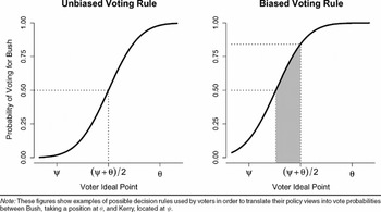
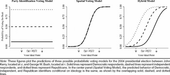
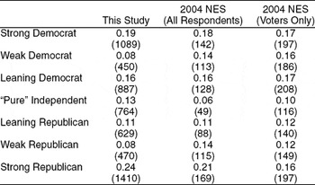
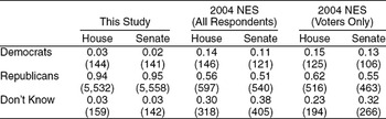
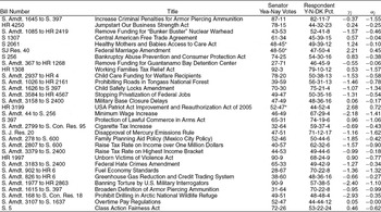
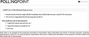
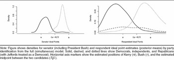
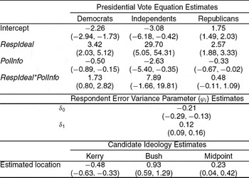
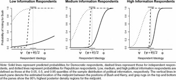
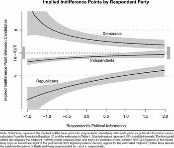



Comments
No Comments have been published for this article.