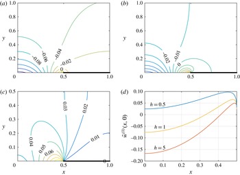
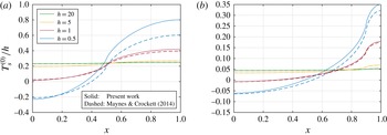
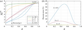
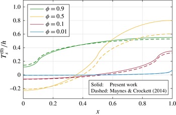
1 Introduction
The use of superhydrophobic surfaces has attracted the attention of many researchers in recent years, due to their ability to reduce flow resistance in microfluidic applications. They are partially non-wetting surfaces consisting of micrometre or sub-micrometre roughness – typically a pattern of grooves, ridges or pillars – that resists a liquid fully wetting the solid substrate. It is possible for a liquid to assume a stable state (the Cassie–Baxter state) in which it only makes contact with the surface at the tips of the structures, and partially rides on a lubricating layer of vapour (and perhaps non-condensible gas) trapped in the cavities. This decrease in liquid–solid contact area results in a reduction in viscous drag, and the notion of apparent hydrodynamic slip.
A geometry of microstructures that has been extensively studied is a periodic array of rectangular ridges and grooves. Ou, Perot & Rothstein (Reference Ou, Perot and Rothstein2004) and Ou & Rothstein (Reference Ou and Rothstein2005) performed experiments in microchannels with ridges aligned parallel (longitudinal) to the flow direction, reporting up to 40 % reductions in flow resistance. Experimental and numerical work by Davies et al. (Reference Davies, Maynes, Webb and Woolford2006) and Maynes et al. (Reference Maynes, Jeffs, Woolford and Webb2007) was conducted for microchannels with ridges aligned parallel and perpendicular (transverse) to the flow respectively, with the greatest drag reduction found for lower Reynolds numbers. Analytical work for flow over such surfaces has been carried out earlier, however, by Philip (Reference Philip1972) and Lauga & Stone (Reference Lauga and Stone2003). Philip (Reference Philip1972) found solutions using conformal mapping theory for Stokes flow over a range of different geometries, including channel flow with longitudinal or transverse ridges on only one wall, and pipe flow with longitudinal ridges. Lauga & Stone (Reference Lauga and Stone2003) found analytical solutions for Stokes flow in a pipe patterned with transverse ridges, using separation of variables. This method was later extended by Teo & Khoo (Reference Teo and Khoo2009) to solve the remaining combinations of transverse/longitudinal ridges on one/both walls for pressure-driven channel flows. In addition to pressure-driven flows, shear-driven flows over ridged surfaces have also been studied (Cottin-Bizonne et al. Reference Cottin-Bizonne, Barentin, Charlaix, Bocquet and Barrat2004; Priezjev, Darhuber & Troian Reference Priezjev, Darhuber and Troian2005; Ybert et al. Reference Ybert, Barentin, Cottin-Bizonne, Joseph and Bocquet2007).
Most of the aforementioned analytical and computational studies have assumed that the liquid–gas interfaces (menisci) are flat for simplicity (or, for the case of pipe flow, that the curvature matches that of the ridge tips). However, the effect of meniscus curvature for parallel-plate channels has also been investigated: analytically for unbounded shear flows over transverse ridges (Davis & Lauga Reference Davis and Lauga2009) and longitudinal ridges (Crowdy Reference Crowdy2010) for large solid fractions; perturbatively for small meniscus protrusion angles and arbitrary solid fractions by Sbragaglia & Prosperetti (Reference Sbragaglia and Prosperetti2007); and numerically for arbitrary angles and solid fractions by Teo & Khoo (Reference Teo and Khoo2010). The latter two studies considered both bounded and unbounded flows. Overall, these studies showed that meniscus curvature can greatly inhibit or enhance the potential slip, depending on whether the interface protrudes into or out of the gas cavities, and the orientation of the ridges. Davis & Lauga found that for transverse ridges, excessive protrusion out of the cavities can cause the slip length to become negative, but this does not occur for longitudinal ridges.
Flows over such surfaces in the presence of heat transfer have received much less attention, but are relevant and of practical and academic interest. The practical interest lies in, e.g., the thermal management of electronics via microchannel cooling of microprocessors, whereby transfer of heat from the solid substrate (silicon) to a liquid coolant is desired, with as little thermal resistance as possible. A significant portion of the total thermal resistance is the caloric resistance of the coolant attributable to the energy required to increase its bulk temperature as it flows through the microchannel (Tuckerman & Pease Reference Tuckerman and Pease1981; Hodes et al.
Reference Hodes, Zhang, Lam, Wilcoxon and Lower2014; Lam, Hodes & Enright Reference Lam, Hodes and Enright2015). The structured walls increase the mass flow rate, and thus decrease the caloric resistance. However, the Nusselt number (
 $Nu$
), which characterises the heat transfer from solid to liquid due to convection, decreases due to less solid–liquid contact area (Enright et al.
Reference Enright, Eason, Dalton, Hodes, Salamon, Kolodner and Krupenkin2006; Maynes, Webb & Davies Reference Maynes, Webb and Davies2008; Maynes et al.
Reference Maynes, Webb, Crockett and Solovjov2013; Maynes & Crockett Reference Maynes and Crockett2014). Thus, evaluation of the net effect of structuring on heat transfer requires evaluation of the caloric and convective resistances, i.e. obtaining of expressions for the slip length and
 $Nu$
for various geometries and physical effects.
A small number of previous studies have considered thermal transport in channels with walls structured with parallel ridges. Enright et al. (Reference Enright, Eason, Dalton, Hodes, Salamon, Kolodner and Krupenkin2006) used an analytical model of the thermal transport in a parallel-plate channel with imposed hydrodynamic slip, neglecting the periodicity of the heating due to the ridge geometry. Maynes et al. (Reference Maynes, Webb and Davies2008) used full numerical simulations to study the case of transverse ridges on both walls, which are held at a constant temperature, while also accounting for heat transfer through the gas cavities. The cases of constant heat flux through ridges oriented transverse and parallel to the flow direction have been studied by Maynes et al. (Reference Maynes, Webb, Crockett and Solovjov2013) and Maynes & Crockett (Reference Maynes and Crockett2014) respectively. Longitudinal ridges were shown in each case to have greater potential for heat transfer enhancement; however, the aforementioned study by Maynes & Crockett did not solve for the velocity field but used a Navier slip approximation, and so neglected the potentially important variation in the velocity near the ridge structures – where the heat is entering (or leaving) the liquid. This effect is captured in the current study, where we calculate the full velocity field, and show that the Navier slip assumption breaks down for geometries where the channel height is comparable to the ridge period. More recently, Enright et al. (Reference Enright, Hodes, Salamon and Muzychka2014) derived Nusselt number expressions in a channel assuming asymmetric hydrodynamic and thermal slip profiles (different slip lengths on opposing walls), imposing constant heat flux, and Cheng, Xu & Sui (Reference Cheng, Xu and Sui2015) investigated the effect of Reynolds number using full numerical simulations, imposing constant temperature. In addition to parallel ridges, both studies also considered structuring with pillars.
Many physical effects at the meniscus can be important to the heat transfer problem, including thermocapillary stresses, evaporation/condensation and meniscus curvature. Thermocapillary stress for flow over ridged surfaces has been considered by Baier, Steffes & Hardt (Reference Baier, Steffes and Hardt2010) and recently by Hodes et al. (Reference Hodes, Kirk, Karamanis, Lam, MacLachlan and Papageorgiou2015a
), and evaporation/condensation has been investigated by Hodes et al. (Reference Hodes, Lam, Cowley, Enright and MacLachlan2015b
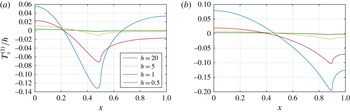
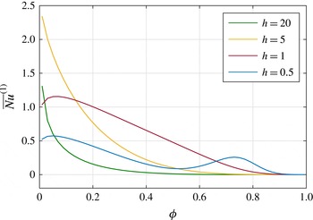
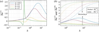
). However, all previous work on heat transfer (including that mentioned in the previous paragraph) has assumed a flat meniscus. Very recently, Lam et al. (Reference Lam, Hodes, Karamanis, Kirk and MacLachlan2016) investigated the effect of meniscus curvature on the thermal problem in a semi-infinite domain, but without convection and therefore interaction with the velocity field. To the best of our knowledge, the effect of meniscus curvature on the convective thermal transport problem in a microchannel has not been considered. This is the primary goal of this paper. We will calculate the Nusselt number for channel flow over longitudinal ridges with constant heat flux, including small meniscus curvature via boundary perturbation. In doing so, for the hydrodynamic problem we will extend the small-curvature analysis of Sbragaglia & Prosperetti (Reference Sbragaglia and Prosperetti2007), who considered longitudinal ridges on one channel wall, to the case of longitudinal ridges on both walls. Additionally, we will bridge the gap between the finite-channel-height solution, requiring a numerical solution of dual series equations, and the analytical semi-infinite shear-driven solution, to provide analytical expressions for the hydrodynamic slip length, accurate even for channel heights comparable to the ridge period. The perturbation will be performed on the full coupled velocity and thermal problems, and the solutions will be determined semi-analytically in terms of eigenfunction expansions. The resulting slip length and Nusselt number will then be presented as functions of the channel geometry. The slip length is accurately described by the asymptotic expressions (6.4), (6.10) and (6.11), whereas the Nusselt-number results are completely captured in a single graph, figure 11(
 $b$
).
In § 2, we formulate both the hydrodynamic and the thermal problems, and the shape and description of the meniscus. Section 3 describes the boundary perturbation method for small curvature, and the resulting mathematical problems at each order. Section 4 details the solutions for the velocity problems, and § 5 the solutions for the temperature problems, with the asymptotic solutions for large channel heights in § 6. The results are then presented in § 7, and conclusions in § 8.
2 Formulation
2.1 Governing equations
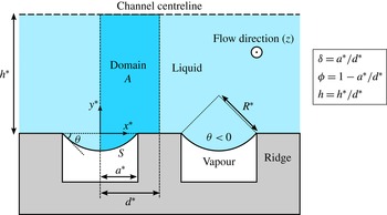
We consider hydrodynamically and thermally fully developed flow in a parallel-plate channel, with uniformly spaced parallel ridges aligned with the flow direction, as in figure 1. The top and bottom walls are structured identically, so that the flow is symmetric about the centre plane of the channel. Surface tension maintains the liquid in the Cassie state, i.e. the liquid contacts the solid substrate only on the tops of the ridges. The grooves between ridges are filled with vapour (and perhaps non-condensible gas). The pressure difference between the liquid and the gas causes the menisci to protrude into (or out of) the cavities. The protrusion is considered to be small enough that the liquid–solid contact angle is small enough for the contact line to stay pinned at the corners of the ridges.
Schematic of the flow configuration, showing the liquid–solid contact and groove dimensions. Domain
 $A$
is the cross-section used for the analysis.

The period of the ridges is denoted by
 $2d^{\ast }$
, the width of each groove by
 $2a^{\ast }$
and the distance from the top of the ridges to the channel centre line by
 $h^{\ast }$
, as shown in figure 1. The use of an asterisk indicates a dimensional quantity. The meniscus protrudes at an angle
 $\unicode[STIX]{x1D703}$
relative to the horizontal at the triple (liquid–solid–gas) contact lines. Positive
 $\unicode[STIX]{x1D703}$
corresponds to protrusion out of the groove. The
 $x^{\ast }$
,
 $y^{\ast }$
and
 $z^{\ast }$
directions are taken to be the spanwise, transverse (wall-normal) and streamwise directions respectively, with
 $x^{\ast }$
and
 $y^{\ast }$
measured from the midpoint between the top of two adjacent ridges. Assuming the number of ridges to be sufficiently large, we can consider the flow to be periodic in the spanwise (
 $x^{\ast }$
) direction, with the same period as the ridges,
 $2d^{\ast }$
. Hence, we only need to consider a single period window, from the centre of one ridge to the next, say
 $|x^{\ast }|\leqslant d^{\ast }$
. In addition, symmetry about the line
 $x^{\ast }=0$
means that we can further restrict attention to just half of a period,
 $0\leqslant x^{\ast }\leqslant d^{\ast }$
. The appropriate flow domain to consider for analysis,
 $A$
, is shown in figure 1, with its bottom boundary consisting of half of one liquid–solid interface and half of one curved meniscus,
 $S$
. Lengths are non-dimensionalised with respect to the width of this domain,
 $d^{\ast }$
, and we introduce the solid fraction,
 $\unicode[STIX]{x1D719}=1-a^{\ast }/d^{\ast }$
, and the complementary cavity fraction,
 $\unicode[STIX]{x1D6FF}=a^{\ast }/d^{\ast }$
. The dimensionless (half) channel height is defined as
 $h=h^{\ast }/d^{\ast }$
. Neglecting thermocapillary stress-induced convection and evaporation/condensation at the meniscus, there will be no transverse or spanwise flow in fully developed conditions; only the streamwise velocity component
 $w^{\ast }$
will be non-zero. We non-dimensionalise
 $w^{\ast }$
by
 $(d^{\ast 2}/\unicode[STIX]{x1D707})(-\text{d}p^{\ast }/\text{d}z^{\ast })$
, a velocity scale based on the prescribed streamwise pressure gradient
 $-\text{d}p^{\ast }/\text{d}z^{\ast }$
, giving
 $$\begin{eqnarray}w=\frac{\unicode[STIX]{x1D707}}{(d^{\ast })^{2}(-\text{d}p^{\ast }/\text{d}z^{\ast })}w^{\ast },\end{eqnarray}$$
where
 $\unicode[STIX]{x1D707}$
is the dynamic viscosity of the liquid. Then, throughout the domain
 $w$
satisfies
 $$\begin{eqnarray}\unicode[STIX]{x1D6FB}^{2}w=-1,\end{eqnarray}$$
where
 $\unicode[STIX]{x1D6FB}^{2}=\unicode[STIX]{x2202}^{2}/\unicode[STIX]{x2202}x^{2}+\unicode[STIX]{x2202}^{2}/\unicode[STIX]{x2202}y^{2}$
is the two-dimensional Laplacian. Symmetry across the left (
 $x=0$
), right
 $(x=1)$
and top (
 $y=h$
) boundaries of the domain
 $A$
translates to the conditions
 $$\begin{eqnarray}\frac{\unicode[STIX]{x2202}w}{\unicode[STIX]{x2202}x}(0,y)=0,\quad \frac{\unicode[STIX]{x2202}w}{\unicode[STIX]{x2202}x}(1,y)=0,\quad \frac{\unicode[STIX]{x2202}w}{\unicode[STIX]{x2202}y}(x,h)=0.\end{eqnarray}$$
On the solid ridge we apply the no-slip condition,
 $$\begin{eqnarray}w(x,0)=0\quad \text{for }\unicode[STIX]{x1D6FF}<x\leqslant 1,\end{eqnarray}$$
while on the meniscus
 $S$
we assume no tangential stress,
 $$\begin{eqnarray}\boldsymbol{n}\boldsymbol{\cdot }\unicode[STIX]{x1D735}w=0\quad \text{on }S,\end{eqnarray}$$
where
 $\boldsymbol{n}$
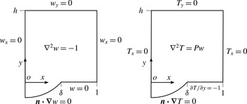
is the unit (outward) normal to the meniscus. The domain, equations and boundary conditions for the
 $w$
(and
 $T$
) problem are summarised in figure 2.
Domains, governing equations and boundary conditions for the
 $w$
and
 $T$
problems. Subscripts denote partial differentiation.

In the thermal problem for the temperature field
 $T^{\ast }$
, we assume that the only source of heating of the liquid is through its contact with the solid ridges, where it experiences a constant heat flux per unit area,
 $q_{sl}^{\prime \prime }$
. Specifically, on the solid–liquid interface we have
 $$\begin{eqnarray}-k\frac{\unicode[STIX]{x2202}T^{\ast }}{\unicode[STIX]{x2202}y^{\ast }}=q_{sl}^{\prime \prime }\quad \text{for }\unicode[STIX]{x1D6FF}<x\leqslant 1.\end{eqnarray}$$
The numerical results of Maynes et al. (Reference Maynes, Webb and Davies2008) show that, for a flat meniscus, the rate of heat conducting into the liquid through the gas cavities is negligible in comparison to the rate entering through the solid ridges for cavity depths greater than approximately 25 % of the cavity width. We will assume this here, and take the gas phase to be adiabatic, applying a zero-heat-flux condition on the meniscus:
 $$\begin{eqnarray}\boldsymbol{n}\boldsymbol{\cdot }\unicode[STIX]{x1D735}T^{\ast }=0\quad \text{on }S.\end{eqnarray}$$
Viscous dissipation, Marangoni induced convection, and evaporation and condensation at the meniscus are neglected. The dimensional thermal energy equation is then
 $$\begin{eqnarray}w^{\ast }\frac{\unicode[STIX]{x2202}T^{\ast }}{\unicode[STIX]{x2202}z^{\ast }}=\unicode[STIX]{x1D6FC}\left(\frac{\unicode[STIX]{x2202}^{2}T^{\ast }}{\unicode[STIX]{x2202}x^{\ast 2}}+\frac{\unicode[STIX]{x2202}^{2}T^{\ast }}{\unicode[STIX]{x2202}y^{\ast 2}}+\frac{\unicode[STIX]{x2202}^{2}T^{\ast }}{\unicode[STIX]{x2202}z^{\ast 2}}\right),\end{eqnarray}$$
where
 $\unicode[STIX]{x1D6FC}=k/(\unicode[STIX]{x1D70C}c_{p})$
is the thermal diffusivity of the liquid,
 $k$
is the thermal conductivity,
 $\unicode[STIX]{x1D70C}$
is the density and
 $c_{p}$
is the specific heat, all assumed to be constant. The thermally fully developed assumption, i.e. that we are sufficiently far from the channel inlet so as to neglect entrance effects, is characterised by the self-similarity property (Bergman et al.
Reference Bergman, Lavine, Incropera and DeWitt2011):
 $$\begin{eqnarray}\frac{\unicode[STIX]{x2202}}{\unicode[STIX]{x2202}z^{\ast }}\left[\frac{T^{\ast }(x^{\ast },y^{\ast },z^{\ast })-T_{sl}^{\ast }(x^{\ast },z^{\ast })}{T_{m}^{\ast }(z^{\ast })-T_{sl}^{\ast }(x^{\ast },z^{\ast })}\right]=0,\end{eqnarray}$$
where
 $T_{sl}^{\ast }$
is the temperature on the solid–liquid interface and
 $T_{m}^{\ast }$
is the mixed-mean liquid temperature,
 $$\begin{eqnarray}T_{m}^{\ast }=\frac{\displaystyle \int _{A}w^{\ast }T^{\ast }\,\text{d}x^{\ast }\,\text{d}y^{\ast }}{\displaystyle \int _{A}w^{\ast }\,\text{d}x^{\ast }\,\text{d}y^{\ast }}.\end{eqnarray}$$
For the constant-heat-flux boundary condition (2.6), the property (2.9) can be shown, conveniently, to imply
 $\unicode[STIX]{x2202}T^{\ast }/\unicode[STIX]{x2202}z^{\ast }=\text{d}T_{m}^{\ast }/\text{d}z^{\ast }=\text{const.}$
As a consequence, the axial conduction term,
 $\unicode[STIX]{x2202}^{2}T^{\ast }/\unicode[STIX]{x2202}z^{\ast 2}$
, is exactly zero and can be dropped from (2.8). The constant can be found by considering an energy balance on a control volume of cross-section
 $A$
and depth
 $\text{d}z^{\ast }$
, yielding
 $$\begin{eqnarray}\frac{\unicode[STIX]{x2202}T^{\ast }}{\unicode[STIX]{x2202}z^{\ast }}=\frac{q_{sl}^{\prime \prime }(d^{\ast }-a^{\ast })}{\unicode[STIX]{x1D70C}Q^{\ast }c_{p}},\end{eqnarray}$$
where
 $Q^{\ast }$
is the total volume flow rate through the cross-section
 $A$
.
We non-dimensionalise temperature by subtracting
 $T_{m}^{\ast }$
and then scaling by the characteristic temperature scale,
 $\unicode[STIX]{x0394}T^{\ast }=q_{sl}^{\prime \prime }d^{\ast }/k$
, from the heat flux condition (2.6), to give
 $$\begin{eqnarray}T=\frac{T^{\ast }-T_{m}^{\ast }}{\unicode[STIX]{x0394}T^{\ast }}=\frac{k(T^{\ast }-T_{m}^{\ast })}{q_{sl}^{\prime \prime }d^{\ast }}.\end{eqnarray}$$
Then, the dimensionless form of the thermal energy equation (2.8) is
 $$\begin{eqnarray}Pw=\unicode[STIX]{x1D6FB}^{2}T,\end{eqnarray}$$
where it is convenient to introduce
 $$\begin{eqnarray}P=\frac{\unicode[STIX]{x1D719}}{Q},\end{eqnarray}$$
with
 $Q$
the non-dimensional flow rate. Thus, the forcing
 $Pw$
is determined completely by the hydrodynamic problem.
Just as with the velocity, the left (
 $x=0$
), right (
 $x=1$
) and top (
 $y=h$
) boundaries of the domain are symmetry boundaries of
 $T$
, and so
 $$\begin{eqnarray}\frac{\unicode[STIX]{x2202}T}{\unicode[STIX]{x2202}x}(0,y)=0,\quad \frac{\unicode[STIX]{x2202}T}{\unicode[STIX]{x2202}x}(1,y)=0,\quad \frac{\unicode[STIX]{x2202}T}{\unicode[STIX]{x2202}y}(x,h)=0.\end{eqnarray}$$
The constant-heat-flux condition (2.6) on the ridge becomes
 $$\begin{eqnarray}\frac{\unicode[STIX]{x2202}T}{\unicode[STIX]{x2202}y}=-1\quad \text{for }\unicode[STIX]{x1D6FF}<x\leqslant 1,\end{eqnarray}$$
and the adiabatic condition on the meniscus (2.7) is unchanged. Just as for the
 $w$
problem, see figure 2 for a summary of the problem for
 $T$
. The
 $w$
problem can be solved in isolation, and then the solution
 $w$
appears as a forcing in the Poisson problem for
 $T$
. It should be noted that this is possible for a meniscus of any shape or curvature.
The quantity that characterises the heat transfer problem is the Nusselt number,
 $Nu$
, which captures the influence of the structured surface (including apparent slip and periodic heating) on the overall thermal transport due to convection. We follow Maynes & Crockett (Reference Maynes and Crockett2014) and define a local Nusselt number
 $$\begin{eqnarray}Nu(x)=\frac{h_{T}(x)D}{k},\end{eqnarray}$$
where
 $D$
is the hydraulic diameter,
 $D=4h^{\ast }$
, and
 $h_{T}(x)$
is the local heat transfer coefficient (not to be confused with
 $h$
, the non-dimensional half-channel thickness), defined as
 $h_{T}(x)=q_{sl}^{\prime \prime }/(T_{sl}^{\ast }-T_{m}^{\ast })$
on the solid–liquid interface (where the temperature is
 $T_{sl}^{\ast }$
) and zero on the meniscus. Hence,
 $$\begin{eqnarray}Nu(x)=\left\{\begin{array}{@{}ll@{}}{\displaystyle \frac{4h}{T_{sl}(x)}},\quad & \text{on solid, }\unicode[STIX]{x1D6FF}<x\leqslant 1,\\ 0,\quad & \text{on meniscus, }0\leqslant x<\unicode[STIX]{x1D6FF}.\end{array}\right.\end{eqnarray}$$
It should be noted that
 $T_{sl}(x)$
is not a function of
 $z$
, which can be shown from the non-dimensionalisation (2.12) and fully developed assumption (2.9). Averaging
 $Nu(x)$
over the composite interface (solid–liquid interface and meniscus) gives the average Nusselt number characterising the structured surface,
 $$\begin{eqnarray}\overline{Nu}=\frac{1}{\unicode[STIX]{x1D719}+|S|}\int _{\unicode[STIX]{x1D6FF}}^{1}Nu(x)\,\text{d}x,\end{eqnarray}$$
where
 $\unicode[STIX]{x1D719}+|S|$
is the total length of the composite interface. This length factor will, however, have no effect on the results in this paper (see (3.25)). We remark that there are other ways of defining a Nusselt number to represent the structured surface, such as using only the temperature at the centre of the ridge, where it will be highest.
2.2 Meniscus curvature
We will take a perturbative approach to investigate the effect of meniscus curvature on the heat transfer problem, based on the assumption that the deflection of the interface relative to a flat one is small. As in Sbragaglia & Prosperetti (Reference Sbragaglia and Prosperetti2007), we represent the position of the meniscus in the form
 $$\begin{eqnarray}y=-\unicode[STIX]{x1D716}\unicode[STIX]{x1D702}(x),\quad 0\leqslant x\leqslant \unicode[STIX]{x1D6FF},\end{eqnarray}$$
where
 $\unicode[STIX]{x1D702}(x)$
is some shape function and
 $\unicode[STIX]{x1D716}$
is the parameter that is taken to be small compared with 1. To relate
 $\unicode[STIX]{x1D716}$
to dimensional quantities and find an expression for
 $\unicode[STIX]{x1D702}(x)$
, we can briefly return to dimensional variables and invoke the Young–Laplace equation relating the capillary pressure difference across a static interface to its radius of curvature. Denoting the pressure on the liquid side of the interface by
 $p_{l}^{\ast }$
, that on the gas side by
 $p_{g}^{\ast }$
and the local radius of curvature by
 $R^{\ast }$
,
 $$\begin{eqnarray}p_{l}^{\ast }-p_{g}^{\ast }=\frac{\unicode[STIX]{x1D70E}}{R^{\ast }},\end{eqnarray}$$
where
 $\unicode[STIX]{x1D70E}$
is the surface tension along the meniscus. As there is no flow in the transverse directions,
 $p_{l}^{\ast }$
is constant throughout any given flow cross-section, and we have neglected the gas phase so will assume that
 $p_{g}^{\ast }$
is constant throughout the length of the cavity. Hence, for a given value of
 $z^{\ast }$
, the difference
 $p_{l}^{\ast }-p_{g}^{\ast }$
is constant along the meniscus, giving a constant radius of curvature. Assuming a small streamwise capillary number, as we move down the channel, the pressure
 $p_{l}^{\ast }$
will fall and
 $R^{\ast }$
will increase, but the change will be slow enough not to invalidate the assumption of locally unidirectional flow (Ou et al.
Reference Ou, Perot and Rothstein2004; Ou & Rothstein Reference Ou and Rothstein2005).
If
 $p_{l}^{\ast }>p_{g}^{\ast }$
, then
 $R^{\ast }>0$
, and the meniscus protrudes into the cavity (negative protrusion angle
 $\unicode[STIX]{x1D703}$
), and if
 $p_{l}^{\ast }<p_{g}^{\ast }$
, then
 $R^{\ast }<0$
, which we can interpret as the meniscus protruding upwards into the liquid (positive protrusion angle
 $\unicode[STIX]{x1D703}$
). In general, both signs of
 $\unicode[STIX]{x1D703}$
are possible since the Young equilibrium angle can lie anywhere between the advancing and receding contact angles.
For protrusion into the cavity, a circle of radius
 $R^{\ast }$
passing through the corners of neighbouring ridges, i.e.
 $x^{\ast }=\pm a^{\ast }$
, is defined by
 $$\begin{eqnarray}y^{\ast }=\sqrt{R^{\ast 2}-a^{\ast 2}}-\sqrt{R^{\ast 2}-x^{\ast 2}}.\end{eqnarray}$$
Defining
 $R=R^{\ast }/d^{\ast }$
, in non-dimensional form this is
 $$\begin{eqnarray}y=\sqrt{R^{2}-\unicode[STIX]{x1D6FF}^{2}}-\sqrt{R^{2}-x^{2}},\end{eqnarray}$$
which when expanded for
 $R\gg 1$
gives
 $$\begin{eqnarray}y=-\frac{1}{2R}(\unicode[STIX]{x1D6FF}^{2}-x^{2})+O\left(\frac{1}{R^{3}}\right).\end{eqnarray}$$
Thus, we define our small parameter as
 $\unicode[STIX]{x1D716}=1/(2R)$
and our shape function as
 $\unicode[STIX]{x1D702}(x)=\unicode[STIX]{x1D6FF}^{2}-x^{2}$
. Then, for
 $\unicode[STIX]{x1D716}\ll 1$
, the meniscus is prescribed by
 $$\begin{eqnarray}y=-\unicode[STIX]{x1D716}\unicode[STIX]{x1D702}(x)+O(\unicode[STIX]{x1D716}^{3}).\end{eqnarray}$$
As we will not calculate up to third order in
 $\unicode[STIX]{x1D716}$
in our perturbative expansion, only first order, the leading-order approximation
 $y=-\unicode[STIX]{x1D716}\unicode[STIX]{x1D702}$
will be sufficient. The case of protrusion into the liquid corresponds to negative
 $\unicode[STIX]{x1D716}$
. The relation between
 $\unicode[STIX]{x1D716}$
and the protrusion angle
 $\unicode[STIX]{x1D703}$
is found from geometry,
 $$\begin{eqnarray}\unicode[STIX]{x1D716}=\frac{1}{2R}=-\frac{\sin \unicode[STIX]{x1D703}}{2\unicode[STIX]{x1D6FF}}.\end{eqnarray}$$
Water on low-surface-energy fluoropolymer has a maximum advancing contact angle of approximately
 $110^{\circ }$
(measured from vertical), corresponding to a maximum (negative) protrusion angle of
 $\unicode[STIX]{x1D703}=-20^{\circ }$
. For low solid fractions, e.g.
 $\unicode[STIX]{x1D719}=1-\unicode[STIX]{x1D6FF}=0.01$
, this gives a maximum value of
 $\unicode[STIX]{x1D716}=0.17$
.
3 Boundary perturbation
The method of analysis we will employ is boundary perturbation, whereby the solution to the problem with a curved meniscus (with small curvature characterised by
 $|\unicode[STIX]{x1D716}|\ll 1$
) is approximated by a hierarchy of problems in powers of
 $\unicode[STIX]{x1D716}$
, each with a flat meniscus. We base the method on that of Sbragaglia & Prosperetti (Reference Sbragaglia and Prosperetti2007), who solved the purely hydrodynamic problem for a similar geometry. If the shape and position of the meniscus are written in the form (with
 $O(\unicode[STIX]{x1D716}^{3})$
error)
 $$\begin{eqnarray}y=-\unicode[STIX]{x1D716}\unicode[STIX]{x1D702}(x),\quad 0\leqslant x\leqslant \unicode[STIX]{x1D6FF},\end{eqnarray}$$
then the vanishing normal derivative condition on the meniscus (2.5) can be written
 $$\begin{eqnarray}\unicode[STIX]{x1D716}\frac{\text{d}\unicode[STIX]{x1D702}}{\text{d}x}\frac{\unicode[STIX]{x2202}w}{\unicode[STIX]{x2202}x}+\frac{\unicode[STIX]{x2202}w}{\unicode[STIX]{x2202}y}=0\quad \text{on }y=-\unicode[STIX]{x1D716}\unicode[STIX]{x1D702}.\end{eqnarray}$$
Since
 $|\unicode[STIX]{x1D716}|\ll 1$
, we Taylor expand the quantities evaluated at
 $y=-\unicode[STIX]{x1D716}\unicode[STIX]{x1D702}$
about
 $y=0$
, assuming that
 $w$
is sufficiently smooth. Taylor expanding
 $w$
, we have
 $$\begin{eqnarray}w(x,-\unicode[STIX]{x1D716}\unicode[STIX]{x1D702})=w(x,0)-\unicode[STIX]{x1D716}\unicode[STIX]{x1D702}\frac{\unicode[STIX]{x2202}w}{\unicode[STIX]{x2202}y}(x,0)+O(\unicode[STIX]{x1D716}^{2}),\end{eqnarray}$$
and, in particular,
 $$\begin{eqnarray}\displaystyle & \displaystyle \frac{\unicode[STIX]{x2202}w}{\unicode[STIX]{x2202}y}(x,-\unicode[STIX]{x1D716}\unicode[STIX]{x1D702}) & \displaystyle =\frac{\unicode[STIX]{x2202}w}{\unicode[STIX]{x2202}y}(x,0)-\unicode[STIX]{x1D716}\unicode[STIX]{x1D702}\frac{\unicode[STIX]{x2202}^{2}w}{\unicode[STIX]{x2202}y^{2}}(x,0)+O(\unicode[STIX]{x1D716}^{2}),\end{eqnarray}$$
 $$\begin{eqnarray}\displaystyle & \displaystyle \frac{\unicode[STIX]{x2202}w}{\unicode[STIX]{x2202}x}(x,-\unicode[STIX]{x1D716}\unicode[STIX]{x1D702}) & \displaystyle =\frac{\unicode[STIX]{x2202}w}{\unicode[STIX]{x2202}x}(x,0)+O(\unicode[STIX]{x1D716}).\end{eqnarray}$$
Substitution into (3.2) gives, up to terms of
 $O(\unicode[STIX]{x1D716})$
,
 $$\begin{eqnarray}\frac{\unicode[STIX]{x2202}w}{\unicode[STIX]{x2202}y}(x,0)-\unicode[STIX]{x1D716}\unicode[STIX]{x1D702}\frac{\unicode[STIX]{x2202}^{2}w}{\unicode[STIX]{x2202}y^{2}}(x,0)+\unicode[STIX]{x1D716}\frac{\text{d}\unicode[STIX]{x1D702}}{\text{d}x}\frac{\unicode[STIX]{x2202}w}{\unicode[STIX]{x2202}x}(x,0)+O(\unicode[STIX]{x1D716}^{2})=0.\end{eqnarray}$$
Then, substituting a regular perturbative expansion of
 $w$
in powers of
 $\unicode[STIX]{x1D716}$
,
 $$\begin{eqnarray}w=w^{(0)}+\unicode[STIX]{x1D716}w^{(1)}+O(\unicode[STIX]{x1D716}^{2}),\end{eqnarray}$$
and equating terms at each order of
 $\unicode[STIX]{x1D716}$
will yield a series of problems for
 $w^{(0)},w^{(1)},\ldots \,$
, each with an interfacial boundary condition now at
 $y=0$
. At
 $O(\unicode[STIX]{x1D716}^{0})$
, equation (3.6) gives
 $$\begin{eqnarray}\unicode[STIX]{x2202}_{y}w^{(0)}(x,0)=0\quad \text{for }0\leqslant x<\unicode[STIX]{x1D6FF},\end{eqnarray}$$
and at
 $O(\unicode[STIX]{x1D716}^{1})$
,
 $$\begin{eqnarray}\unicode[STIX]{x2202}_{y}w^{(1)}(x,0)=\unicode[STIX]{x1D702}\unicode[STIX]{x2202}_{yy}w^{(0)}(x,0)-\unicode[STIX]{x1D702}^{\prime }\unicode[STIX]{x2202}_{x}w^{(0)}(x,0)\quad \text{for }0\leqslant x<\unicode[STIX]{x1D6FF},\end{eqnarray}$$
where, for brevity, we denote
 $\unicode[STIX]{x2202}_{y}=\unicode[STIX]{x2202}/\unicode[STIX]{x2202}y$
,
 $\unicode[STIX]{x2202}_{yy}=\unicode[STIX]{x2202}^{2}/\unicode[STIX]{x2202}y^{2}$
and
 $\unicode[STIX]{x1D702}^{\prime }=\text{d}\unicode[STIX]{x1D702}/\text{d}x$
. The governing equation, (2.2), gives
 $$\begin{eqnarray}\unicode[STIX]{x1D6FB}^{2}w^{(0)}=-1\end{eqnarray}$$
at
 $O(\unicode[STIX]{x1D716}^{0})$
and
 $$\begin{eqnarray}\unicode[STIX]{x1D6FB}^{2}w^{(1)}=0\end{eqnarray}$$
at
 $O(\unicode[STIX]{x1D716}^{1})$
(and at all higher orders). The no-slip condition on the solid ridge (2.4) and the symmetry conditions (2.3) are satisfied at all orders, and thus by
 $w^{(0)}$
and
 $w^{(1)}$
.
The boundary perturbation analysis for the temperature field
 $T$
is similar to that for the velocity field, and is expressed as
 $$\begin{eqnarray}T=T^{(0)}+\unicode[STIX]{x1D716}T^{(1)}+O(\unicode[STIX]{x1D716}^{2}).\end{eqnarray}$$
The meniscus condition (2.7) is identical to that for
 $w$
, thus
 $$\begin{eqnarray}\displaystyle & \unicode[STIX]{x2202}_{y}T^{(0)}(x,0)=0,\quad 0\leqslant x<\unicode[STIX]{x1D6FF}, & \displaystyle\end{eqnarray}$$
 $$\begin{eqnarray}\displaystyle & \unicode[STIX]{x2202}_{y}T^{(1)}(x,0)=\unicode[STIX]{x1D702}\unicode[STIX]{x2202}_{yy}T^{(0)}(x,0)-\unicode[STIX]{x1D702}^{\prime }\unicode[STIX]{x2202}_{x}T^{(0)}(x,0),\quad 0\leqslant x<\unicode[STIX]{x1D6FF}, & \displaystyle\end{eqnarray}$$
and the symmetry boundary conditions (2.15) are satisfied at all orders. Only the boundary condition on the ridge and the governing equation differ from those of the velocity problem. The constant-heat-flux boundary condition on the ridge,
 $\unicode[STIX]{x2202}T/\unicode[STIX]{x2202}y=-1$
, gives
 $$\begin{eqnarray}\displaystyle & \unicode[STIX]{x2202}_{y}T^{(0)}=-1,\quad \unicode[STIX]{x1D6FF}<x\leqslant 1, & \displaystyle\end{eqnarray}$$
 $$\begin{eqnarray}\displaystyle & \unicode[STIX]{x2202}_{y}T^{(1)}=0,\quad \unicode[STIX]{x1D6FF}<x\leqslant 1. & \displaystyle\end{eqnarray}$$
It should be recalled that
 $T$
satisfies Poisson’s equation (2.13) with forcing
 $Pw$
, where
 $P=\unicode[STIX]{x1D719}/Q$
. Hence, we must expand the flow rate
 $Q$
. When
 $\unicode[STIX]{x1D716}>0$
,
 $$\begin{eqnarray}\displaystyle Q & = & \displaystyle \displaystyle \int _{0}^{1}\int _{0}^{h}w(x,y;\unicode[STIX]{x1D716})\,\text{d}y\,\text{d}x+\int _{0}^{\unicode[STIX]{x1D6FF}}\int _{-\unicode[STIX]{x1D716}\unicode[STIX]{x1D702}}^{0}w(x,y;\unicode[STIX]{x1D716})\,\text{d}y\,\text{d}x,\end{eqnarray}$$
 $$\begin{eqnarray}\displaystyle & = & \displaystyle Q^{(0)}+\unicode[STIX]{x1D716}(Q_{1}^{(1)}+Q_{2}^{(1)})+O(\unicode[STIX]{x1D716}^{2}),\end{eqnarray}$$
where
 $$\begin{eqnarray}\displaystyle & \displaystyle Q^{(0)}=\int _{0}^{h}\int _{0}^{1}w^{(0)}(x,y)\,\text{d}x\,\text{d}y, & \displaystyle\end{eqnarray}$$
 $$\begin{eqnarray}\displaystyle & \displaystyle Q_{1}^{(1)}=\int _{0}^{h}\int _{0}^{1}w^{(1)}(x,y)\,\text{d}x\,\text{d}y, & \displaystyle\end{eqnarray}$$
 $$\begin{eqnarray}\displaystyle & \displaystyle Q_{2}^{(1)}=\int _{0}^{\unicode[STIX]{x1D6FF}}w^{(0)}(x,0)\unicode[STIX]{x1D702}(x)\,\text{d}x. & \displaystyle\end{eqnarray}$$
If
 $\unicode[STIX]{x1D716}<0$
, the integral definition of
 $Q$
cannot be split up as in (3.17), but the resulting expansion (3.18) is the same. Thus, (3.18) holds for both positive and negative
 $\unicode[STIX]{x1D716}$
. We can interpret
 $Q_{1}^{(1)}$
as the
 $O(\unicode[STIX]{x1D716})$
contribution to the flow rate due to the change in the velocity field, and
 $Q_{2}^{(1)}$
as the
 $O(\unicode[STIX]{x1D716})$
contribution due to the change in cross-sectional area of the domain. Then, the expansion
 $P=P^{(0)}+\unicode[STIX]{x1D716}P^{(1)}+O(\unicode[STIX]{x1D716}^{2})$
of
 $P=\unicode[STIX]{x1D719}/Q$
up to
 $O(\unicode[STIX]{x1D716})$
is given by
 $$\begin{eqnarray}\displaystyle P^{(0)}=\frac{\unicode[STIX]{x1D719}}{Q^{(0)}},\quad P^{(1)}=-P^{(0)}\frac{Q_{1}^{(1)}+Q_{2}^{(1)}}{Q^{(0)}}. & & \displaystyle\end{eqnarray}$$
Substitution of the expansions for
 $T$
,
 $w$
and
 $P$
into
 $\unicode[STIX]{x1D6FB}^{2}T=Pw$
gives
 $$\begin{eqnarray}\displaystyle & \unicode[STIX]{x1D6FB}^{2}T^{(0)}=P^{(0)}w^{(0)}\quad \text{at }O(\unicode[STIX]{x1D716}^{0}), & \displaystyle\end{eqnarray}$$
 $$\begin{eqnarray}\displaystyle & \unicode[STIX]{x1D6FB}^{2}T^{(1)}=P^{(0)}w^{(1)}+P^{(1)}w^{(0)}\quad \text{at }O(\unicode[STIX]{x1D716}^{1}). & \displaystyle\end{eqnarray}$$
Finally, expanding
 $\overline{Nu}=\overline{Nu}^{(0)}+\unicode[STIX]{x1D716}\overline{Nu}^{(1)}+O(\unicode[STIX]{x1D716}^{2})$
,
 $$\begin{eqnarray}\displaystyle \overline{Nu}^{(0)}=\int _{\unicode[STIX]{x1D6FF}}^{1}\frac{4h}{T_{s}^{(0)}}\,\text{d}x,\quad \overline{Nu}^{(1)}=-\int _{\unicode[STIX]{x1D6FF}}^{1}\frac{4hT_{s}^{(1)}}{(T_{s}^{(0)})^{2}}\,\text{d}x. & & \displaystyle\end{eqnarray}$$
The length of the composite interface, i.e. the factor of
 $\unicode[STIX]{x1D719}+|S|$
in (2.19), is simply
 $1+O(\unicode[STIX]{x1D716}^{2})$
, so the increase in length is an
 $O(\unicode[STIX]{x1D716}^{2})$
effect and does not affect the analysis in this paper.
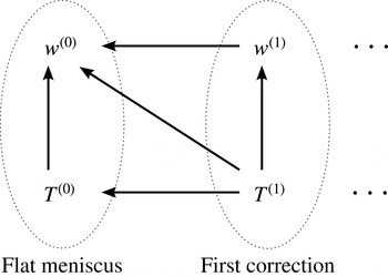
The four fields and their dependences on each other are shown in figure 3. We will solve for them in the following order. The velocity problem can be solved independently of the temperature problem, and hence we will solve it first, for
 $w^{(0)}$
and then for
 $w^{(1)}$
. Knowledge of
 $w^{(0)}$
allows us to solve for
 $T^{(0)}$
, and finally knowledge of
 $w^{(0)},w^{(1)}$
and
 $T^{(0)}$
is needed to solve for
 $T^{(1)}$
.
Schematic of the four fields to be found. The arrows denote dependences, i.e. ‘is forced by’.

4 Velocity problem,
 $w$

The velocity problem considered here is similar to the one solved by Sbragaglia & Prosperetti (Reference Sbragaglia and Prosperetti2007). However, whereas they considered the case of longitudinal ridges on one channel wall and a flat plate with the no-slip boundary condition on the other, we are considering the symmetric case of ridges on both channel walls. Mathematically, this means that we have the symmetry condition
 $\unicode[STIX]{x2202}_{y}w=0$
instead of
 $w=0$
at the top (
 $y=h$
) of our domain. The cases will coincide in the limit of a semi-infinite channel,
 $h\rightarrow \infty$
.
4.1 Zeroth-order solution,
$w^{(0)}$

The problem for
 $w^{(0)}$
is
 $$\begin{eqnarray}\displaystyle & \unicode[STIX]{x1D6FB}^{2}w^{(0)}=-1,\quad 0<x<1,\quad 0<y<h, & \displaystyle\end{eqnarray}$$
 $$\begin{eqnarray}\displaystyle & \unicode[STIX]{x2202}_{y}w^{(0)}(x,0)=0,\quad 0\leqslant x<\unicode[STIX]{x1D6FF}, & \displaystyle\end{eqnarray}$$
 $$\begin{eqnarray}\displaystyle & w^{(0)}(x,0)=0,\quad \unicode[STIX]{x1D6FF}<x\leqslant 1, & \displaystyle\end{eqnarray}$$
along with vanishing normal derivatives on the remaining boundaries,
 $$\begin{eqnarray}\unicode[STIX]{x2202}_{x}w^{(0)}(0,y)=\unicode[STIX]{x2202}_{x}w^{(0)}(1,y)=\unicode[STIX]{x2202}_{y}w^{(0)}(x,h)=0.\end{eqnarray}$$
We will solve for
 $w^{(0)}$
in the form of an eigenfunction expansion, and the solution is provided by, e.g., Teo & Khoo (Reference Teo and Khoo2009). We write the solution as the one-dimensional flow profile (satisfying Poisson’s equation and no-slip on
 $y=0$
) and a perturbation part:
 $$\begin{eqnarray}w^{(0)}=-{\textstyle \frac{1}{2}}y^{2}+hy+h\tilde{w}^{(0)}.\end{eqnarray}$$
Then,
 $\tilde{w}^{(0)}$
satisfies Laplace’s equation, with a constant shear stress on the flat meniscus,
 $$\begin{eqnarray}\displaystyle & \unicode[STIX]{x1D6FB}^{2}\tilde{w}^{(0)}=0,\quad 0<x<1,\quad 0<y<h, & \displaystyle\end{eqnarray}$$
 $$\begin{eqnarray}\displaystyle & \unicode[STIX]{x2202}_{y}\tilde{w}^{(0)}(x,0)=-1,\quad 0\leqslant x<\unicode[STIX]{x1D6FF}, & \displaystyle\end{eqnarray}$$
 $$\begin{eqnarray}\displaystyle & \tilde{w}^{(0)}(x,0)=0,\quad \unicode[STIX]{x1D6FF}<x\leqslant 1, & \displaystyle\end{eqnarray}$$
along with the symmetry conditions (4.4). Using separation of variables, or noting that
 $\tilde{w}^{(0)}$
is even in
 $x$
with period
 $2$
, the solution can be written as a Fourier cosine series in
 $x$
,
 $$\begin{eqnarray}\tilde{w}^{(0)}(x,y)=a_{0}^{(0)}+\mathop{\sum }_{n=1}^{\infty }a_{n}^{(0)}\frac{\cosh [k_{n}(y-h)]}{\cosh (k_{n}h)}\cos (k_{n}x),\end{eqnarray}$$
where
 $k_{n}=n\unicode[STIX]{x03C0}$
. It should be noted that this satisfies the requirement that
 $\unicode[STIX]{x2202}_{y}\tilde{w}^{(0)}=0$
at
 $y=h$
. The coefficients,
 $a_{n}^{(0)}$
, are then determined from the conditions on the composite interface, equations (4.7) and (4.8), which lead to the dual series equations
 $$\begin{eqnarray}\displaystyle & \displaystyle a_{0}^{(0)}+\mathop{\sum }_{n=1}^{\infty }a_{n}^{(0)}\cos (k_{n}x)=0,\quad \unicode[STIX]{x1D6FF}<x<1, & \displaystyle\end{eqnarray}$$
 $$\begin{eqnarray}\displaystyle & \displaystyle \mathop{\sum }_{n=1}^{\infty }a_{n}^{(0)}k_{n}\tanh (k_{n}h)\cos (k_{n}x)=1,\quad 0<x<\unicode[STIX]{x1D6FF}. & \displaystyle\end{eqnarray}$$
In the limit of a channel of infinite height,
 $h\rightarrow \infty$
, these can be solved analytically (see § 6), but for a finite channel they must be solved numerically. The numerical method used is the same as that of previous authors (Lauga & Stone Reference Lauga and Stone2003; Sbragaglia & Prosperetti Reference Sbragaglia and Prosperetti2007; Teo & Khoo Reference Teo and Khoo2009), and is outlined in an appendix of Sbragaglia & Prosperetti (Reference Sbragaglia and Prosperetti2007). Briefly, the method is to truncate each series at
 $n=N$
, and then project each equation, in the region where it holds, onto the eigenfunctions
 $\{\cos (k_{n}x):0\leqslant n\leqslant N\}$
to form an (
 $N+1$
)-dimensional linear algebra problem for
 $\boldsymbol{a}^{(0)}=(a_{0}^{(0)},a_{1}^{(0)},\ldots ,a_{N}^{(0)})^{T}\in \mathbb{R}^{N+1}$
, written as
 $\unicode[STIX]{x1D648}\boldsymbol{a}=\boldsymbol{f}$
. The series structure (left-hand sides) and the forcing (right-hand sides) of (4.10)–(4.11) determine
 $\unicode[STIX]{x1D648}\in \mathbb{R}^{N+1}\times \mathbb{R}^{N+1}$
and
 $\boldsymbol{f}\in \mathbb{R}^{N+1}$
respectively.
From this solution, the leading-order flow rate
 $Q^{(0)}$
is found by integrating (4.5) over the rectangular domain, giving
 $$\begin{eqnarray}Q^{(0)}={\textstyle \frac{1}{3}}h^{3}+h^{2}a_{0}^{(0)},\end{eqnarray}$$
and hence
 $$\begin{eqnarray}P^{(0)}=\frac{\unicode[STIX]{x1D719}}{{\textstyle \frac{1}{3}}h^{3}+h^{2}a_{0}^{(0)}}.\end{eqnarray}$$
Lastly, from differentiating the series solution (4.9) term by term,
 $$\begin{eqnarray}\displaystyle \unicode[STIX]{x2202}_{yy}\tilde{w}^{(0)}(x,0) & = & \displaystyle \mathop{\sum }_{n=1}^{\infty }a_{n}^{(0)}k_{n}^{2}\cos (k_{n}x)\nonumber\\ \displaystyle & = & \displaystyle -\unicode[STIX]{x2202}_{xx}\tilde{w}^{(0)}(x,0).\end{eqnarray}$$
Hence,
 $\unicode[STIX]{x1D6FB}^{2}\tilde{w}^{(0)}=0$
and (via (4.5))
 $\unicode[STIX]{x1D6FB}^{2}w^{(0)}=-1$
are satisfied on the meniscus,
 $y=0$
, as well as in the interior of the domain. This justifies simplifying the meniscus boundary condition (3.9) for
 $w^{(1)}$
in the manner of Sbragaglia & Prosperetti (Reference Sbragaglia and Prosperetti2007) to give condition (4.16) below.
4.2 First-order solution,
$w^{(1)}$

The problem for the first-order perturbation
 $w^{(1)}$
is
 $$\begin{eqnarray}\displaystyle & \unicode[STIX]{x1D6FB}^{2}w^{(1)}=0,\quad 0<x<1,\quad 0<y<h, & \displaystyle\end{eqnarray}$$
 $$\begin{eqnarray}\displaystyle & \unicode[STIX]{x2202}_{y}w^{(1)}(x,0)=-\unicode[STIX]{x2202}_{x}[\unicode[STIX]{x1D702}\unicode[STIX]{x2202}_{x}w^{(0)}(x,0)]-\unicode[STIX]{x1D702},\quad 0\leqslant x<\unicode[STIX]{x1D6FF}, & \displaystyle\end{eqnarray}$$
 $$\begin{eqnarray}\displaystyle & w^{(1)}(x,0)=0,\quad \unicode[STIX]{x1D6FF}<x\leqslant 1, & \displaystyle\end{eqnarray}$$
along with vanishing normal derivatives on the remaining boundaries,
 $$\begin{eqnarray}\unicode[STIX]{x2202}_{x}w^{(1)}(0,y)=\unicode[STIX]{x2202}_{x}w^{(1)}(1,y)=\unicode[STIX]{x2202}_{y}w^{(1)}(x,h)=0.\end{eqnarray}$$
We write the solution in a similar form to
 $w^{(0)}$
, but a one-dimensional base profile is unnecessary, i.e.
 $w^{(1)}=h\tilde{w}^{(1)}$
. Then,
 $\tilde{w}^{(1)}$
can also be written as a Fourier series,
 $$\begin{eqnarray}\tilde{w}^{(1)}(x,y)=a_{0}^{(1)}+\mathop{\sum }_{n=1}^{\infty }a_{n}^{(1)}\frac{\cosh [k_{n}(y-h)]}{\cosh (k_{n}h)}\cos (k_{n}x).\end{eqnarray}$$
The no-slip condition (4.17) and meniscus condition (4.16) give another set of dual series equations,
 $$\begin{eqnarray}\displaystyle & \displaystyle a_{0}^{(1)}+\mathop{\sum }_{n=1}^{\infty }a_{n}^{(1)}\cos (k_{n}x)=0,\quad \unicode[STIX]{x1D6FF}<x<1, & \displaystyle\end{eqnarray}$$
 $$\begin{eqnarray}\displaystyle & \displaystyle \mathop{\sum }_{n=1}^{\infty }a_{n}^{(1)}k_{n}\tanh (k_{n}h)\cos (k_{n}x)=\unicode[STIX]{x2202}_{x}(\unicode[STIX]{x1D702}\unicode[STIX]{x2202}_{x}\tilde{w}^{(0)}(x,0))+\frac{\unicode[STIX]{x1D702}}{h},\quad 0<x<\unicode[STIX]{x1D6FF}. & \displaystyle\end{eqnarray}$$
This system for
 $a_{n}^{(1)}$
takes the same form as for
 $a_{n}^{(0)}$
, with the only difference being the forcing on the right-hand side of the second equation (4.21). Again, this can be solved analytically in the limit
 $h\rightarrow \infty$
(see § 6), but for finite
 $h$
we must solve this numerically.
Once
 $a_{n}^{(0)}$
and
 $a_{n}^{(1)}$
are computed, the changes to the flow rate,
 $Q_{1}^{(1)}$
and
 $Q_{2}^{(1)}$
, can be calculated by inserting the series (4.19) and (4.9) into (4.22) and (4.23) respectively. Then,
 $$\begin{eqnarray}\displaystyle & Q_{1}^{(1)}=h^{2}a_{0}^{(1)}, & \displaystyle\end{eqnarray}$$
 $$\begin{eqnarray}\displaystyle & \displaystyle Q_{2}^{(1)}=\frac{2}{3}\unicode[STIX]{x1D6FF}^{3}ha_{0}^{(0)}+h\mathop{\sum }_{n=1}^{\infty }a_{n}^{(0)}\int _{0}^{\unicode[STIX]{x1D6FF}}\unicode[STIX]{x1D702}(x)\cos k_{n}x\,\text{d}x, & \displaystyle\end{eqnarray}$$
where each integral in the last sum can be calculated using integration by parts and
 $\unicode[STIX]{x1D702}(x)=\unicode[STIX]{x1D6FF}^{2}-x^{2}$
to give
 $$\begin{eqnarray}\int _{0}^{\unicode[STIX]{x1D6FF}}\unicode[STIX]{x1D702}(x)\cos k_{n}x\,\text{d}x=\frac{2\sin k_{n}\unicode[STIX]{x1D6FF}}{k_{n}^{3}}-\frac{2\unicode[STIX]{x1D6FF}\cos k_{n}\unicode[STIX]{x1D6FF}}{k_{n}^{2}}.\end{eqnarray}$$
We can define an apparent slip length by equating the flow rate
 $Q$
with what it would be,
 $Q_{\mathit{slip}}$
, if the ridges were replaced with a flat surface subjected to a Navier slip condition,
 $w_{\mathit{slip}}(x,0)=\unicode[STIX]{x1D706}\unicode[STIX]{x2202}_{y}w_{\mathit{slip}}(x,0)$
, from which we find
 $$\begin{eqnarray}Q_{\mathit{slip}}={\textstyle \frac{1}{3}}h^{3}+h^{2}\unicode[STIX]{x1D706}.\end{eqnarray}$$
Here,
 $\unicode[STIX]{x1D706}$
is the slip length normalised by half the ridge period, i.e.
 $\unicode[STIX]{x1D706}=\unicode[STIX]{x1D706}^{\ast }/d^{\ast }$
. We expand
 $\unicode[STIX]{x1D706}$
similarly to
 $Q$
,
 $$\begin{eqnarray}\unicode[STIX]{x1D706}=\unicode[STIX]{x1D706}^{(0)}+\unicode[STIX]{x1D716}(\unicode[STIX]{x1D706}_{1}^{(1)}+\unicode[STIX]{x1D706}_{2}^{(1)})+O(\unicode[STIX]{x1D716}^{2}),\end{eqnarray}$$
where
 $\unicode[STIX]{x1D706}^{(0)}$
,
 $\unicode[STIX]{x1D706}_{1}^{(1)}$
and
 $\unicode[STIX]{x1D706}_{2}^{(1)}$
are the contributions from
 $Q^{(0)},Q_{1}^{(1)}$
and
 $Q_{2}^{(1)}$
respectively. Thus, using (4.25), (4.12), (4.22) and (4.23), we find
 $$\begin{eqnarray}\displaystyle & \unicode[STIX]{x1D706}^{(0)}=a_{0}^{(0)}, & \displaystyle\end{eqnarray}$$
 $$\begin{eqnarray}\displaystyle & \unicode[STIX]{x1D706}_{1}^{(1)}=a_{0}^{(1)}, & \displaystyle\end{eqnarray}$$
 $$\begin{eqnarray}\displaystyle & \displaystyle \unicode[STIX]{x1D706}_{2}^{(1)}=\frac{2}{3}\frac{\unicode[STIX]{x1D6FF}^{3}}{h}a_{0}^{(0)}+\frac{1}{h}\mathop{\sum }_{n=1}^{\infty }a_{n}^{(0)}\left(\frac{2\sin k_{n}\unicode[STIX]{x1D6FF}}{k_{n}^{3}}-\frac{2\unicode[STIX]{x1D6FF}\cos k_{n}\unicode[STIX]{x1D6FF}}{k_{n}^{2}}\right). & \displaystyle\end{eqnarray}$$
5 Temperature problem,
$T$

Now that we have determined the velocity field,
 $w=w^{(0)}+\unicode[STIX]{x1D716}w^{(1)}+O(\unicode[STIX]{x1D716}^{2})$
, up to first order, we can solve for the temperature field up to the same order,
 $T=T^{(0)}+\unicode[STIX]{x1D716}T^{(1)}+O(\unicode[STIX]{x1D716}^{2})$
. It should be recalled that the perturbation of the thermal problem and equating orders of
 $\unicode[STIX]{x1D716}$
was carried out at the beginning of § 3, to give problems for
 $T^{(0)}$
and
 $T^{(1)}$
, which we repeat below. The leading-order thermal problem, corresponding to the case of a flat meniscus, has been solved by Maynes & Crockett (Reference Maynes and Crockett2014) using a one-dimensional approximation of the velocity field, but not with the exact two-dimensional velocity field, as we will do here. The first-order problem for
 $T^{(1)}$
, quantifying the effect of curvature on heat transfer in microchannels, has not to the best of our knowledge been considered before, except very recently for the case of a semi-infinite (
 $h=\infty$
) domain with no advection (
 $w\equiv 0$
) (Lam et al.
Reference Lam, Hodes, Karamanis, Kirk and MacLachlan2016).
5.1 Zeroth-order solution,
$T^{(0)}$

The problem for
 $T^{(0)}$
, the temperature for the case of a flat meniscus, is given by (see (2.13))
 $$\begin{eqnarray}\displaystyle & \unicode[STIX]{x1D6FB}^{2}T^{(0)}=P^{(0)}w^{(0)},\quad 0<x<1,\quad 0<y<h, & \displaystyle\end{eqnarray}$$
 $$\begin{eqnarray}\displaystyle & \unicode[STIX]{x2202}_{y}T^{(0)}(x,0)=0,\quad 0\leqslant x<\unicode[STIX]{x1D6FF}, & \displaystyle\end{eqnarray}$$
 $$\begin{eqnarray}\displaystyle & \unicode[STIX]{x2202}_{y}T^{(0)}(x,0)=-1,\quad \unicode[STIX]{x1D6FF}<x\leqslant 1, & \displaystyle\end{eqnarray}$$
along with vanishing normal derivatives on the remaining boundaries,
 $$\begin{eqnarray}\unicode[STIX]{x2202}_{x}T^{(0)}(0,y)=\unicode[STIX]{x2202}_{x}T^{(0)}(1,y)=\unicode[STIX]{x2202}_{y}T^{(0)}(x,h)=0.\end{eqnarray}$$
It should be recalled that
 $P^{(0)}=\unicode[STIX]{x1D719}/Q^{(0)}=\unicode[STIX]{x1D719}/(1/3h^{3}+h^{2}a_{0}^{(0)})$
, and
 $w^{(0)}$
is given by (4.5) and (4.9). Substitution of
 $w^{(0)}$
into (5.1) gives
 $$\begin{eqnarray}\unicode[STIX]{x1D6FB}^{2}T^{(0)}=P^{(0)}\left\{-\frac{1}{2}y^{2}+hy+ha_{0}^{(0)}+h\mathop{\sum }_{n=1}^{\infty }a_{n}^{(0)}\frac{\cosh [k_{n}(y-h)]}{\cosh (k_{n}h)}\cos (k_{n}x)\right\},\end{eqnarray}$$
and we see that the forcing consists of a quadratic in
 $y$
plus an infinite series, each term in the series depending on both
 $x$
and
 $y$
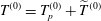
. This can be handled by setting
 $T^{(0)}=T_{p}^{(0)}+\widetilde{T}^{(0)}$
, i.e. splitting it into a particular solution,
 $T_{p}^{(0)}$
, that satisfies the forcing and a remaining homogeneous (harmonic) part,
 $\widetilde{T}^{(0)}$
, that enforces the boundary conditions on the composite interface,
 $y=0$
. In addition, if
 $T_{p}^{(0)}$
satisfies the symmetry properties across
 $x=0$
,
 $x=1$
and
 $y=h$
, then
 $\widetilde{T}^{(0)}$
will also. To find such a
 $T_{p}^{(0)}$
, satisfying
 $\unicode[STIX]{x1D6FB}^{2}T_{p}^{(0)}=P^{(0)}w^{(0)}$
and the symmetry conditions, we can consider the two parts of the forcing
 $P^{(0)}w^{(0)}$
separately and then linearly superimpose their solutions. The polynomial part of this forcing,
 $P^{(0)}(-1/2y^{2}+hy+ha_{0}^{(0)}),$
is satisfied by the quartic solution
 $$\begin{eqnarray}P^{(0)}\left[-{\textstyle \frac{1}{24}}(y-h)^{4}+{\textstyle \frac{1}{2}}\left({\textstyle \frac{1}{2}}h^{2}+ha_{0}^{(0)}\right)(y-h)^{2}\right],\end{eqnarray}$$
which is even about the channel centreline,
 $y=h$
, and
 $x=0,1$
. In the infinite series part of the forcing, each term takes a form proportional to
 $\cosh [k_{n}(y-h)]\cos (k_{n}x),$
and so the particular solution in this case is
 $$\begin{eqnarray}f_{n}(x,y):=\frac{(y-h)\sinh [k_{n}(y-h)]}{2k_{n}}\cos (k_{n}x),\end{eqnarray}$$
which is also even about
 $y=h$
and
 $x=0,1$
. It should be noted that each series term in the forcing is harmonic, so each corresponding particular solution
 $f_{n}$
is biharmonic (
 $\unicode[STIX]{x1D6FB}^{4}f_{n}=0$
). Thus,
 $f_{n}$
can also be found from the biharmonic general solution in Cartesian coordinates, and enforcing
 $\unicode[STIX]{x1D6FB}^{2}f_{n}=\cosh (k_{n}(y-h))\cos (k_{n}x)$
and symmetry. Finally, combining all of these components, we find
 $$\begin{eqnarray}\displaystyle T_{p}^{(0)} & = & \displaystyle P^{(0)}\left[-\frac{1}{24}(y-h)^{4}+\frac{1}{2}\left(\frac{1}{2}h^{2}+ha_{0}^{(0)}\right)(y-h)^{2}\right.\nonumber\\ \displaystyle & & \displaystyle +\left.\mathop{\sum }_{n=1}^{\infty }\frac{ha_{n}^{(0)}}{2k_{n}}\frac{(y-h)\sinh (k_{n}(y-h))}{\cosh (k_{n}h)}\cos (k_{n}x)\right],\end{eqnarray}$$
which satisfies (5.1). Recalling that
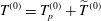 $T^{(0)}=T_{p}^{(0)}+\widetilde{T}^{(0)}$
, the remaining part,
 $\widetilde{T}^{(0)}$
, then satisfies the homogeneous equation
 $$\begin{eqnarray}\displaystyle \unicode[STIX]{x1D6FB}^{2}\widetilde{T}^{(0)}=0,\quad 0<x<1,\quad 0<y<h, & & \displaystyle\end{eqnarray}$$
but with a modification to the condition on
 $y=0$
, which can be written as
 $\unicode[STIX]{x2202}_{y}\widetilde{T}^{(0)}(x,0)=-H(x-\unicode[STIX]{x1D6FF})-\unicode[STIX]{x2202}_{y}T_{p}^{(0)}(x,0)$
, or
 $$\begin{eqnarray}\unicode[STIX]{x2202}_{y}\widetilde{T}^{(0)}(x,0)=-H(x-\unicode[STIX]{x1D6FF})+P^{(0)}\left\{Q^{(0)}+\mathop{\sum }_{n=1}^{\infty }\frac{ha_{n}^{(0)}}{2k_{n}}[\tanh (k_{n}h)+k_{n}h]\cos (k_{n}x)\right\},\end{eqnarray}$$
where
 $H(x)$
is the Heaviside step function. Lastly,
 $\widetilde{T}^{(0)}$
satisfies the symmetry conditions (5.4).
Just as for the previous Laplace problems (4.6) and (4.15),
 $\widetilde{T}^{(0)}$
has a series solution,
 $$\begin{eqnarray}\widetilde{T}^{(0)}=b_{0}^{(0)}+\mathop{\sum }_{n=1}^{\infty }b_{n}^{(0)}\frac{\cosh [k_{n}(y-h)]}{\cosh (k_{n}h)}\cos (k_{n}x),\end{eqnarray}$$
and the coefficients
 $b_{n}^{(0)}$
can be determined from the condition (5.10) at
 $y=0$
. The problems for
 $\tilde{w}^{(0)}$
and
 $\tilde{w}^{(1)}$
had mixed Dirichlet and Neumann conditions at
 $y=0$
, and resulted in dual series equations. The condition (5.10) for
 $\widetilde{T}^{(0)}$
is not mixed, only discontinuous, and so can be handled in the usual way by substituting (5.11) into condition (5.10), then multiplying by
 $\cos (k_{m}x)$
and integrating over
 $x\in [0,1]$
. The result is
 $$\begin{eqnarray}\displaystyle b_{m}^{(0)}=\frac{\coth (k_{m}h)}{k_{m}}\left\{-\frac{2\sin (k_{m}\unicode[STIX]{x1D6FF})}{k_{m}}-\frac{P^{(0)}ha_{m}^{(0)}}{2k_{m}}[\tanh (k_{m}h)+k_{m}h]\right\},\quad m=1,2,\ldots . & & \displaystyle\end{eqnarray}$$
It should be noted that since the boundary condition is in terms of
 $\unicode[STIX]{x2202}_{y}\widetilde{T}^{(0)}$
, it cannot determine the first coefficient,
 $b_{0}^{(0)}$
. Instead, it is fixed by enforcing the zero-mixed-mean condition,
 $T_{m}=0$
, which to leading order is
 $$\begin{eqnarray}\int _{0}^{h}\int _{0}^{1}w^{(0)}T^{(0)}\text{d}x\,\text{d}y=0.\end{eqnarray}$$
This holds because we used the mixed mean in the definition of
 $T$
as per (2.12). Substituting the series expressions for
 $w^{(0)}$
and
 $T^{(0)}$
, and then using orthogonality and integration by parts gives
 $$\begin{eqnarray}\displaystyle b_{0}^{(0)} & = & \displaystyle -\frac{1}{Q^{(0)}}\left\{P^{(0)}\left[\frac{1}{336}h^{7}-\frac{7}{120}\left(\frac{1}{2}h^{2}+ha_{0}^{(0)}\right)h^{5}+\frac{1}{6}\left(\frac{1}{2}h^{2}+ha_{0}^{(0)}\right)^{2}h^{3}\right]\right.\nonumber\\ \displaystyle & & \displaystyle +\,\mathop{\sum }_{n=1}^{\infty }\frac{P^{(0)}h^{2}(a_{n}^{(0)})^{2}}{4k_{n}}\left[\frac{h}{4k_{n}}(2-\text{sech}^{2}(k_{n}h))-\frac{1}{4k_{n}^{2}}\tanh (k_{n}h)\right]\nonumber\\ \displaystyle & & \displaystyle \left.+\,\mathop{\sum }_{n=1}^{\infty }\frac{ha_{n}^{(0)}b_{n}^{(0)}}{2}\left[\frac{1}{2}h\,\text{sech}^{2}(k_{n}h)+\frac{1}{2k_{n}}\tanh (k_{n}h)\right]\right\}.\end{eqnarray}$$
Therefore, given the Fourier coefficients
 $a_{n}^{(0)}$
of the velocity field
 $w^{(0)}$
, the temperature field
 $T^{(0)}$
can be decomposed into a particular solution
 $T_{p}^{(0)}$
, given explicitly by (5.8), and a Fourier series
 $\widetilde{T}^{(0)}$
, with coefficients given explicitly by (5.12) and (5.14).
Setting
 $y=0$
in expressions (5.8) and (5.11) then gives the temperature
 $T_{s}^{(0)}(x)$
on the composite interface,
 $$\begin{eqnarray}\displaystyle T_{s}^{(0)}(x) & = & \displaystyle P^{(0)}\left[-\frac{1}{24}h^{4}+\frac{1}{2}\left(\frac{1}{2}h^{2}+ha_{0}^{(0)}\right)h^{2}+\mathop{\sum }_{n=1}^{\infty }\frac{h^{2}a_{n}^{(0)}}{2k_{n}}\tanh (k_{n}h)\cos (k_{n}x)\right]\nonumber\\ \displaystyle & & \displaystyle +\,b_{0}^{(0)}+\mathop{\sum }_{n=1}^{\infty }b_{n}^{(0)}\cos (k_{n}x).\end{eqnarray}$$
The local and average Nusselt numbers are given by
 $Nu^{(0)}(x)=4h/T_{s}^{(0)}(x)$
and
 $\overline{Nu}^{(0)}=\int _{\unicode[STIX]{x1D6FF}}^{1}4h/T_{s}^{(0)}\,\text{d}x$
, with the integration performed numerically.
5.2 First-order solution,
$T^{(1)}$

In this section, we develop the first-order correction,
 $T^{(1)}$
, to the temperature field due to the curvature of the meniscus. From § 3, the problem for
 $T^{(1)}$
is
 $$\begin{eqnarray}\displaystyle & \unicode[STIX]{x1D6FB}^{2}T^{(1)}=P^{(1)}w^{(0)}+P^{(0)}w^{(1)},\quad 0<x<1,\quad 0<y<h, & \displaystyle\end{eqnarray}$$
 $$\begin{eqnarray}\displaystyle & \unicode[STIX]{x2202}_{y}T^{(1)}(x,0)=\unicode[STIX]{x1D702}\unicode[STIX]{x2202}_{yy}T^{(0)}(x,0)-\unicode[STIX]{x1D702}^{\prime }\unicode[STIX]{x2202}_{x}T^{(0)}(x,0),\quad 0\leqslant x<\unicode[STIX]{x1D6FF}, & \displaystyle\end{eqnarray}$$
 $$\begin{eqnarray}\displaystyle & \unicode[STIX]{x2202}_{y}T^{(1)}(x,0)=0,\quad \unicode[STIX]{x1D6FF}<x\leqslant 1, & \displaystyle\end{eqnarray}$$
along with vanishing normal derivatives on the remaining boundaries,
 $$\begin{eqnarray}\unicode[STIX]{x2202}_{x}T^{(1)}(0,y)=\unicode[STIX]{x2202}_{x}T^{(1)}(1,y)=\unicode[STIX]{x2202}_{y}T^{(1)}(x,h)=0.\end{eqnarray}$$
Here,
 $P^{(0)}$
and
 $P^{(1)}$
are constants given by (3.22), in terms of the flow rates
 $Q^{(0)}$
,
 $Q_{1}^{(1)}$
and
 $Q_{2}^{(1)}$
of the velocity problem. It should be noted that the boundary condition (5.17) for
 $T^{(1)}$
on the meniscus comes from expanding the normal derivative condition
 $\boldsymbol{n}\boldsymbol{\cdot }\unicode[STIX]{x1D735}T=0$
, and so takes the same form as that for
 $w^{(1)}$
, (3.9). The condition (5.17) can be simplified in a similar fashion to (3.9) by noting from the series solution that
 $\unicode[STIX]{x1D6FB}^{2}T^{(0)}=P^{(0)}w^{(0)}$
applies not only in the domain interior but also on
 $y=0$
,
 $0\leqslant x<\unicode[STIX]{x1D6FF}$
(excluding the triple contact line, i.e.
 $y=0$
,
 $x=\unicode[STIX]{x1D6FF}$
). Thus, (5.17) can be written
 $$\begin{eqnarray}\displaystyle \unicode[STIX]{x2202}_{y}T^{(1)}(x,0)=-\unicode[STIX]{x2202}_{x}[\unicode[STIX]{x1D702}\unicode[STIX]{x2202}_{x}T^{(0)}(x,0)]+\unicode[STIX]{x1D702}P^{(0)}w^{(0)}(x,0),\quad 0\leqslant x<\unicode[STIX]{x1D6FF}. & & \displaystyle\end{eqnarray}$$
To proceed, we take the same approach that we took for
 $T^{(0)}$
, and set
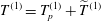 $T^{(1)}=T_{p}^{(1)}+\widetilde{T}^{(1)}$
, where
 $T_{p}^{(1)}$
is the particular solution that satisfies the forcing in (5.16), and
 $\widetilde{T}^{(1)}$
is a remaining homogeneous (harmonic) part that enforces the conditions at
 $y=0$
. In (5.16), the first forcing term,
 $P^{(1)}w^{(0)}$
, is the same as at the previous order, (5.1), with
 $P^{(0)}$
replaced with
 $P^{(1)}$
. The second term,
 $P^{(0)}w^{(1)}$
, is similar, but with
 $w^{(0)}$
replaced with
 $w^{(1)}$
, which has the same Fourier series structure. Thus, we can construct
 $T_{p}^{(1)}$
from two copies of
 $T_{p}^{(0)}$
, with the above changes made. It can be verified that
 $$\begin{eqnarray}\displaystyle T_{p}^{(1)} & = & \displaystyle P^{(1)}\left[-\frac{1}{24}(y-h)^{4}+\frac{1}{4}h^{2}(y-h)^{2}\right]+\frac{1}{2}h(P^{(1)}a_{0}^{(0)}+P^{(0)}a_{0}^{(1)})(y-h)^{2}\nonumber\\ \displaystyle & & \displaystyle +\,\mathop{\sum }_{n=1}^{\infty }\frac{h}{2k_{n}}(P^{(1)}a_{n}^{(0)}+P^{(0)}a_{n}^{(1)})\frac{(y-h)\sinh [k_{n}(y-h)]}{\cosh (k_{n}h)}\cos (k_{n}x)\end{eqnarray}$$
satisfies
 $\unicode[STIX]{x1D6FB}^{2}T_{p}^{(1)}=P^{(1)}w^{(0)}+P^{(0)}w^{(1)}$
, and the symmetry conditions (5.19). The remaining part,
 $\widetilde{T}^{(1)}$
, in the decomposition then satisfies the homogeneous problem
 $$\begin{eqnarray}\displaystyle \unicode[STIX]{x1D6FB}^{2}\widetilde{T}^{(1)}=0,\quad 0<x<1,\quad 0<y<h, & & \displaystyle\end{eqnarray}$$
but with the following modification to the conditions on
 $y=0$
:
 $$\begin{eqnarray}\displaystyle \unicode[STIX]{x2202}_{y}\widetilde{T}^{(1)}(x,0)=H(x-\unicode[STIX]{x1D6FF})[\unicode[STIX]{x1D702}P^{(0)}w^{(0)}(x,0)-\unicode[STIX]{x2202}_{x}(\unicode[STIX]{x1D702}\unicode[STIX]{x2202}_{x}T^{(0)}(x,0))]-\unicode[STIX]{x2202}_{y}T_{p}^{(1)}(x,0), & & \displaystyle\end{eqnarray}$$
where the last term is from differentiating (5.21). Similarly to the previous Laplace problems (
 $\tilde{w}^{(0)}$
,
 $\tilde{w}^{(1)}$
, and
 $\widetilde{T}^{(0)}$
),
 $\widetilde{T}^{(1)}$
has a series solution
 $$\begin{eqnarray}\widetilde{T}^{(1)}=b_{0}^{(1)}+\mathop{\sum }_{n=1}^{\infty }b_{n}^{(1)}\frac{\cosh [k_{n}(y-h)]}{\cosh (k_{n}h)}\cos (k_{n}x),\end{eqnarray}$$
and the
 $b_{n}^{(1)}$
are found from condition (5.23) by substituting (5.21), then multiplying by
 $\cos (k_{m}x)$
(for
 $m\geqslant 1$
) and integrating
 $x\in [0,1]$
, giving
 $$\begin{eqnarray}\displaystyle b_{m}^{(1)} & = & \displaystyle \coth (k_{m}h)\left[\frac{4h}{k_{m}}P^{(0)}a_{0}^{(0)}\left(\frac{\unicode[STIX]{x1D6FF}\cos (k_{m}\unicode[STIX]{x1D6FF})}{k_{m}^{2}}-\frac{\sin (k_{m}\unicode[STIX]{x1D6FF})}{k_{m}^{3}}\right)-\mathop{\sum }_{n\geqslant 1}\frac{2h}{k_{m}}P^{(0)}a_{n}^{(0)}\tilde{\unicode[STIX]{x1D613}}_{mn}\right.\nonumber\\ \displaystyle & & \displaystyle \left.-\mathop{\sum }_{n\geqslant 1}(h^{2}P^{(0)}a_{n}^{(0)}\tanh (k_{n}h)+2k_{n}b_{n}^{(0)})\unicode[STIX]{x1D613}_{mn}\right]\nonumber\\ \displaystyle & & \displaystyle -\,\frac{h}{2k_{m}^{2}}(P^{(1)}a_{m}^{(0)}+P^{(0)}a_{m}^{(1)})[1+k_{m}h\coth (k_{m}h)],\quad m=1,2,\ldots ,\end{eqnarray}$$
where
 $\unicode[STIX]{x1D613}_{mn}=\int _{0}^{\unicode[STIX]{x1D6FF}}\unicode[STIX]{x1D702}(x)\cos (k_{m}x)\cos (k_{n}x)\,\text{d}x$
and
 $\tilde{\unicode[STIX]{x1D613}}_{mn}=\int _{0}^{\unicode[STIX]{x1D6FF}}\unicode[STIX]{x1D702}(x)\sin (k_{m}x)\sin (k_{n}x)\,\text{d}x$
are known matrices, given by (A 1) and (A 2) respectively (see appendix A). As with
 $\widetilde{T}^{(0)}$
, the coefficient
 $b_{0}^{(1)}$
is fixed by the zero-mixed-mean condition. Expanding this condition for
 $0<\unicode[STIX]{x1D716}\ll 1$
,
 $$\begin{eqnarray}\displaystyle 0 & = & \displaystyle \int _{A}w(x,y;\unicode[STIX]{x1D716})T(x,y;\unicode[STIX]{x1D716})\,\text{d}x\,\text{d}y\nonumber\\ \displaystyle & = & \displaystyle \int _{0}^{h}\int _{0}^{1}wT\,\text{d}x\,\text{d}y+\int _{0}^{\unicode[STIX]{x1D6FF}}\int _{-\unicode[STIX]{x1D716}\unicode[STIX]{x1D702}}^{0}wT\,\text{d}y\,\text{d}x\nonumber\\ \displaystyle & = & \displaystyle \int _{0}^{h}\int _{0}^{1}w^{(0)}T^{(0)}\,\text{d}x\,\text{d}y+\unicode[STIX]{x1D716}\int _{0}^{h}\int _{0}^{1}(w^{(0)}T^{(1)}+w^{(1)}T^{(0)})\,\text{d}x\,\text{d}y\nonumber\\ \displaystyle & & \displaystyle +\,\unicode[STIX]{x1D716}\int _{0}^{\unicode[STIX]{x1D6FF}}\unicode[STIX]{x1D702}w^{(0)}(x,0)T^{(0)}(x,0)\,\text{d}x+O(\unicode[STIX]{x1D716}^{2}).\end{eqnarray}$$
At
 $O(\unicode[STIX]{x1D716}^{0})$
this recovers (5.13), and at
 $O(\unicode[STIX]{x1D716}^{1})$
we have
 $$\begin{eqnarray}0=\int _{0}^{h}\int _{0}^{1}(w^{(0)}T^{(1)}+w^{(1)}T^{(0)})\,\text{d}x\,\text{d}y+\int _{0}^{\unicode[STIX]{x1D6FF}}\unicode[STIX]{x1D702}w^{(0)}(x,0)T^{(0)}(x,0)\,\text{d}x.\end{eqnarray}$$
Substitution of our series solutions for
 $w^{(0)}$
,
 $w^{(1)}$
,
 $T^{(0)}$
and
 $T^{(1)}$
gives an expression for
 $b_{0}^{(1)}$
. The computation is straightforward but long, and the expression for
 $b_{0}^{(1)}$
is unwieldy, so the details can be found in appendix B. Despite this, the expression (B 7) for
 $b_{0}^{(1)}$
is explicit and is given exactly in terms of the velocity coefficients,
 $a_{n}^{(0)}$
and
 $a_{n}^{(1)}$
, and the geometric parameters
 $h$
and
 $\unicode[STIX]{x1D719}$
(or
 $\unicode[STIX]{x1D6FF}=1-\unicode[STIX]{x1D719}$
).
Defining
 $T_{s}^{(1)}(x):=T^{(1)}(x,0)$
, the corrections to the local and average Nusselt numbers are found numerically from
 $Nu^{(1)}=-4hT_{s}^{(1)}/(T_{s}^{(0)})^{2}$
and
 $\overline{Nu}^{(1)}=-\int _{\unicode[STIX]{x1D6FF}}^{1}4hT_{s}^{(1)}/(T_{s}^{(0)})^{2}\,\text{d}x$
respectively.
6 Asymptotic solution for
$h\rightarrow \infty$

In addition to the solution for arbitrary channel height
 $h$
, a simple yet accurate asymptotic solution in the limit
 $h\rightarrow \infty$
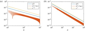
can be found. With the goal of avoiding numerical solution of the dual series equations, which converge very slowly (see figure 13), we seek explicit asymptotic solutions for
 $\unicode[STIX]{x1D706}=\unicode[STIX]{x1D706}^{(0)}+\unicode[STIX]{x1D716}(\unicode[STIX]{x1D706}_{1}^{(1)}+\unicode[STIX]{x1D706}_{2}^{(1)})+\cdots \,$
and
 $\overline{Nu}=\overline{Nu}^{(0)}+\unicode[STIX]{x1D716}\overline{Nu}^{(1)}+\cdots \,$
, now assuming that the channel height is large. As
 $h\rightarrow \infty$
, an asymptotic expansion of each quantity in powers of
 $h^{-1}$
would capture all algebraic dependence on
 $h$
, albeit neglecting exponentially small terms. The resulting limits of
 $w^{(0)},w^{(1)},T^{(0)}$
and
 $T^{(1)}$
will depend on whether
 $y=O(1)$
or
 $y=O(h)$
as
 $h\rightarrow \infty$
. If
 $y=O(1)$
,
 $y$
is fixed on the scale of the ridge period. If
 $y=O(h)$
, then
 $y$
is fixed on the scale of (half) the channel height, and so remains in the central bulk of the channel as
 $h\rightarrow \infty$
. In the language of matched asymptotic expansions, the former is the ‘inner region’ and the latter is the ‘outer region’. The following can be derived formally by constructing asymptotic solutions in each region and matching, or by taking
 $h\rightarrow \infty$
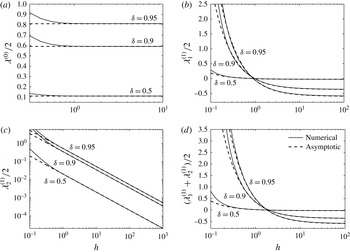
in the solutions already presented and neglecting exponentially small terms. For brevity, we will present the latter approach. A remarkable finding of this analysis is that a two-term asymptotic expansion for the slip length is accurate with exponentially small errors. As a result, we produce formulae that are shown to be accurate for
 $h$
as small as 0.5, making them useful for engineering applications.
6.1 Zeroth-order velocity
First, consider the dual series equations (4.10)–(4.11) for
 $a_{n}^{(0)}$
. The part of (4.11) preventing an analytical solution is the
 $\tanh (n\unicode[STIX]{x03C0}h)$
factor appearing in the sum. However,
 $\tanh (n\unicode[STIX]{x03C0}h)\sim 1+\text{e.s.t.}$
as
 $h\rightarrow \infty$
, where ‘e.s.t.’ denotes ‘exponentially small terms’. Therefore, by replacing
 $\tanh (n\unicode[STIX]{x03C0}h)$
with 1, the equations are those for a semi-infinite channel (coefficients denoted
 $a_{n}^{(0,\infty )}$
) solved by Sbragaglia & Prosperetti (Reference Sbragaglia and Prosperetti2007). Thus,
 $a_{n}^{(0)}\sim a_{n}^{(0,\infty )}+\text{e.s.t.}$
For
 $y=O(1)$
(the inner region), taking
 $h\rightarrow \infty$
in the solution (4.5) for
 $w^{(0)}$
,
 $$\begin{eqnarray}w^{(0)}\sim h(y+\tilde{w}^{(0,\infty )})-{\textstyle \frac{1}{2}}y^{2}+\text{e.s.t.},\quad \text{as }h\rightarrow \infty ,\end{eqnarray}$$
where
 $$\begin{eqnarray}\tilde{w}^{(0,\infty )}(x,y)=a_{0}^{(0,\infty )}+\mathop{\sum }_{n=1}^{\infty }a_{n}^{(0,\infty )}\text{e}^{-n\unicode[STIX]{x03C0}y}\cos (n\unicode[STIX]{x03C0}x).\end{eqnarray}$$
We note that
 $\tilde{w}^{(0,\infty )}$
is the perturbation to the shear-driven flow in a semi-infinite domain, with slip length
 $\unicode[STIX]{x1D706}^{(0,\infty )}=a_{0}^{(0,\infty )}$
, given by Philip (Reference Philip1972),
 $$\begin{eqnarray}\tilde{w}^{(0,\infty )}(x,y)=\text{Im}\left\{\frac{2}{\unicode[STIX]{x03C0}}\cos ^{-1}\left[\frac{\cos \left({\displaystyle \frac{\unicode[STIX]{x03C0}z}{2}}\right)}{\cos \left({\displaystyle \frac{\unicode[STIX]{x03C0}\unicode[STIX]{x1D6FF}}{2}}\right)}\right]\right\},\quad \text{where }z=x+\text{i}y.\end{eqnarray}$$
In particular,
 $$\begin{eqnarray}\displaystyle & \displaystyle a_{0}^{(0,\infty )}=\frac{2}{\unicode[STIX]{x03C0}}\log \left[\sec \left(\frac{\unicode[STIX]{x03C0}\unicode[STIX]{x1D6FF}}{2}\right)\right], & \displaystyle\end{eqnarray}$$
 $$\begin{eqnarray}\displaystyle & \displaystyle \tilde{w}^{(0,\infty )}(x,0)=\frac{2}{\unicode[STIX]{x03C0}}\cosh ^{-1}\left[\frac{\cos \left({\displaystyle \frac{\unicode[STIX]{x03C0}x}{2}}\right)}{\cos \left({\displaystyle \frac{\unicode[STIX]{x03C0}\unicode[STIX]{x1D6FF}}{2}}\right)}\right],\quad 0\leqslant x<\unicode[STIX]{x1D6FF}, & \displaystyle\end{eqnarray}$$
 $$\begin{eqnarray}\displaystyle & \displaystyle \frac{\unicode[STIX]{x2202}\tilde{w}}{\unicode[STIX]{x2202}x}^{(0,\infty )}(x,0)=-\frac{\sqrt{2}\sin \left({\displaystyle \frac{\unicode[STIX]{x03C0}x}{2}}\right)}{\sqrt{\cos \unicode[STIX]{x03C0}x-\cos \unicode[STIX]{x03C0}\unicode[STIX]{x1D6FF}}},\quad 0\leqslant x<\unicode[STIX]{x1D6FF}. & \displaystyle\end{eqnarray}$$
For
 $y=O(h)$
(the outer region), we write
 $y=hY$
with
 $Y=O(1)$
(in fact
 $Y\leqslant 1$
due to the geometry of the problem). In this region, the sum in
 $w^{(0)}$
is exponentially small, so
 $$\begin{eqnarray}w^{(0)}\sim -{\textstyle \frac{1}{2}}h^{2}Y^{2}+h^{2}Y+ha_{0}^{(0,\infty )}+\text{e.s.t.},\quad h\rightarrow \infty ,\end{eqnarray}$$
which is the Navier slip velocity profile.
6.2 First-order velocity
Using
 $\tanh (n\unicode[STIX]{x03C0}h)\sim 1+\text{e.s.t.}$
and
 $\tilde{w}^{(0)}(x,0)\sim \tilde{w}^{(0,\infty )}(x,0)+\text{e.s.t.}$
in the dual series equations (4.20)–(4.21) for
 $a_{n}^{(1)}$
, we obtain
 $$\begin{eqnarray}\displaystyle & \displaystyle a_{0}^{(1)}+\mathop{\sum }_{n=1}^{\infty }a_{n}^{(1)}\cos (n\unicode[STIX]{x03C0}x)=0,\quad \unicode[STIX]{x1D6FF}<x<1, & \displaystyle\end{eqnarray}$$
 $$\begin{eqnarray}\displaystyle & \displaystyle \mathop{\sum }_{n=1}^{\infty }a_{n}^{(1)}n\unicode[STIX]{x03C0}\cos (n\unicode[STIX]{x03C0}x)=\unicode[STIX]{x2202}_{x}(\unicode[STIX]{x1D702}\unicode[STIX]{x2202}_{x}\tilde{w}^{(0,\infty )}(x,0))+\frac{\unicode[STIX]{x1D702}}{h}+\text{e.s.t.},\quad 0<x<\unicode[STIX]{x1D6FF}. & \displaystyle\end{eqnarray}$$
These can now also be solved analytically, in the manner of Sbragaglia & Prosperetti (Reference Sbragaglia and Prosperetti2007), to give
 $$\begin{eqnarray}\displaystyle \unicode[STIX]{x1D706}_{1}^{(1)} & = & \displaystyle a_{0}^{(1)}\sim \underbrace{-\unicode[STIX]{x1D6FF}^{3}\int _{0}^{1}\frac{[1-\cos (\unicode[STIX]{x1D6FF}\unicode[STIX]{x03C0}s)](1-s^{2})\,\text{d}s}{\cos (\unicode[STIX]{x1D6FF}\unicode[STIX]{x03C0}s)-\cos (\unicode[STIX]{x1D6FF}\unicode[STIX]{x03C0})}}_{\displaystyle a_{0}^{(1,\infty )}}+\frac{1}{h}\sqrt{2}\unicode[STIX]{x1D6FF}^{4}\int _{0}^{1}\frac{s(1-s^{2}/3)\sin (\unicode[STIX]{x1D6FF}\unicode[STIX]{x03C0}s/2)\,\text{d}s}{\sqrt{\cos (\unicode[STIX]{x1D6FF}\unicode[STIX]{x03C0}s)-\cos (\unicode[STIX]{x1D6FF}\unicode[STIX]{x03C0})}}\nonumber\\ \displaystyle & & \displaystyle +\,\text{e.s.t.},\quad h\rightarrow \infty .\end{eqnarray}$$
Sbragaglia & Prosperetti only obtained the first term,
 $a_{0}^{(1,\infty )}$
, producing an
 $O(h^{-1})$
error. However, if the
 $O(h^{-1})$
term is captured, as above, the error is exponentially small – a remarkable improvement. The solution of (6.8)–(6.9) can then be used in asymptotic expressions for
 $w^{(1)}$
in the inner and outer regions, just as for
 $w^{(0)}$
.
Lastly, an exponentially accurate expression for
 $\unicode[STIX]{x1D706}_{2}^{(1)}$
, the slip due to the increase in cross-sectional area, is given by
 $$\begin{eqnarray}\displaystyle \unicode[STIX]{x1D706}_{2}^{(1)} & {\sim} & \displaystyle \frac{1}{h}\int _{0}^{\unicode[STIX]{x1D6FF}}\tilde{w}^{(0,\infty )}(x,0)\unicode[STIX]{x1D702}(x)\,\text{d}x+\text{e.s.t.},\nonumber\\ \displaystyle & = & \displaystyle \frac{1}{h}\sqrt{2}\unicode[STIX]{x1D6FF}^{4}\int _{0}^{1}\frac{s(1-s^{2}/3)\sin (\unicode[STIX]{x1D6FF}\unicode[STIX]{x03C0}s/2)\,\text{d}s}{\sqrt{\cos (\unicode[STIX]{x1D6FF}\unicode[STIX]{x03C0}s)-\cos (\unicode[STIX]{x1D6FF}\unicode[STIX]{x03C0})}}+\text{e.s.t.},\end{eqnarray}$$
which is
 $O(h^{-1})$
and, remarkably, identical to the second term in the expression (6.10) for
 $\unicode[STIX]{x1D706}_{1}^{(1)}$
. Thus,
 $\unicode[STIX]{x1D706}^{(1)}=\unicode[STIX]{x1D706}_{1}^{(1)}+\unicode[STIX]{x1D706}_{2}^{(1)}\sim a_{0}^{(1,\infty )}+2\unicode[STIX]{x1D706}_{2}^{(1)}$
.
6.3 Nusselt numbers
Neglecting only exponentially small terms, inner and outer asymptotic solutions as
 $h\rightarrow \infty$
can be found for the temperature field in a similar manner to the velocity field, but the results are not as useful. For exponential accuracy, or even to go further than
 $O(h^{-1})$
in the expansion, however, the full solution to the dual series equations (6.8)–(6.9) is needed, which we only know numerically (analytically we only know
 $a_{0}^{(1)}$
in the limit
 $h\rightarrow \infty$
). Using the asymptotic behaviours
 $a_{0}^{(0)}\sim \unicode[STIX]{x1D706}^{(0,\infty )}+\text{e.s.t}$
,
 $a_{n}^{(0)}\sim a_{n}^{(0,\infty )}+\text{e.s.t}$
,
 $P^{(0)}\sim \unicode[STIX]{x1D719}/(h^{3}/3+h^{2}\unicode[STIX]{x1D706}^{(0,\infty )})+\text{e.s.t.}$
from the velocity problem in the series expression (5.15) for
 $T_{s}^{(0)}(x)$
, we find (after dividing by
 $h$
)
 $$\begin{eqnarray}\frac{1}{h}T_{s}^{(0)}(x)=\frac{17}{35}\unicode[STIX]{x1D719}-\frac{18}{35}\frac{\unicode[STIX]{x1D719}}{h}\unicode[STIX]{x1D706}^{(0,\infty )}+\frac{1}{h}\mathop{\sum }_{n=1}^{\infty }b_{n}^{(0,\infty )}\cos (n\unicode[STIX]{x03C0}x)+O\left(\frac{1}{h^{2}}\right).\end{eqnarray}$$
Here,
 $b_{n}^{(0,\infty )}$
is the leading order of
 $b_{n}^{(0)}$
as
 $h\rightarrow \infty$
, and
 $b_{n}^{(0)}\sim b_{n}^{(0,\infty )}+O(h^{-1})\sim -2\sin (n\unicode[STIX]{x03C0}\unicode[STIX]{x1D6FF})/(n\unicode[STIX]{x03C0})^{2}+O(h^{-1})$
. Substituting into (3.25), expanding further for
 $h\rightarrow \infty$
and integrating, we find, correct to
 $O(h^{-1})$
,
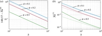
 $$\begin{eqnarray}\overline{Nu}^{(0)}\sim \frac{140}{17}\left[1+\frac{1}{h}\frac{35}{17}\left(\frac{18}{35}\unicode[STIX]{x1D706}^{(0,\infty )}-\mathop{\sum }_{n=1}^{\infty }\frac{2\sin ^{2}(n\unicode[STIX]{x03C0}\unicode[STIX]{x1D6FF})}{\unicode[STIX]{x1D719}^{2}(n\unicode[STIX]{x03C0})^{3}}\right)\right]+O\left(\frac{1}{h^{2}}\right).\end{eqnarray}$$
Moreover, using the behaviour of
 $a_{0}^{(1)}$
,
 $a_{n}^{(1)}$
and
 $b_{n}^{(1)}$
as
 $h\rightarrow \infty$
in the series expression for
 $T_{s}^{(1)}(x)$
, and then substituting into (3.25), we find, after some algebra,
 $$\begin{eqnarray}\overline{Nu}^{(1)}\sim \left(\frac{35}{17}\right)^{2}\frac{4}{h}\left[\frac{18}{35}a_{0}^{(1,\infty )}+\mathop{\sum }_{n=1}^{\infty }\frac{b_{n}^{(1,\infty )}\sin ^{2}(n\unicode[STIX]{x03C0}\unicode[STIX]{x1D6FF})}{\unicode[STIX]{x1D719}^{2}n\unicode[STIX]{x03C0}}\right]+O\left(\frac{1}{h^{2}}\right),\end{eqnarray}$$
where
 $$\begin{eqnarray}b_{n}^{(1,\infty )}=4\mathop{\sum }_{n=1}^{\infty }\unicode[STIX]{x1D613}_{nm}\frac{\sin (m\unicode[STIX]{x03C0}\unicode[STIX]{x1D6FF})}{m\unicode[STIX]{x03C0}},\end{eqnarray}$$
 $\unicode[STIX]{x1D706}^{(0,\infty )}=a_{0}^{(0,\infty )}$
is (6.4),
 $a_{0}^{(1,\infty )}$
is in (6.10) and
 $\unicode[STIX]{x1D613}_{nm}$
is given by (A 1). Despite only
 $O(h^{-1})$
accuracy, these expressions are explicit, with only the sums requiring evaluation.
7 Results and discussion
In this section, we present results for the effect of meniscus curvature on the slip length and Nusselt number, representative of the velocity and temperature problems respectively. At both orders in
 $\unicode[STIX]{x1D716}$
, we quantify the dependence on the slip fraction
 $\unicode[STIX]{x1D6FF}$
(or equivalently the solid fraction
 $\unicode[STIX]{x1D719}=1-\unicode[STIX]{x1D6FF}$
) and the channel height
 $h$
, and assess the accuracy of the asymptotic solutions for
 $h\rightarrow \infty$
.
7.1 Apparent slip length
In the literature, results for the slip length are usually presented normalised by the period, so we will present the quantity
 $\unicode[STIX]{x1D706}^{\ast }/2d^{\ast }=\unicode[STIX]{x1D706}/2$
. Figure 4 shows plots of the slip lengths
 $\unicode[STIX]{x1D706}^{(0)}$
,
 $\unicode[STIX]{x1D706}_{1}^{(1)}$
,
 $\unicode[STIX]{x1D706}_{2}^{(1)}$
(normalised by ridge period) against the channel height
 $h$
, for various slip fractions
 $\unicode[STIX]{x1D6FF}$
. Also shown, as dashed lines, are the asymptotic solutions for
 $h\rightarrow \infty$
, given by (6.4), (6.10) and (6.11). The numerical and asymptotic solutions agree extremely well: less than 1 % difference is typically achieved by
 $h=1$
for
 $\unicode[STIX]{x1D706}^{(0)}$
, and already by
 $h=0.5$
for
 $\unicode[STIX]{x1D706}_{1}^{(1)}$
and
 $\unicode[STIX]{x1D706}_{2}^{(1)}$
. This attests to the exponential accuracy of the asymptotic solutions. The asymptotics should be exact in the limit
 $h\rightarrow \infty$
, and the slight difference seen to persist in the curves for
 $\unicode[STIX]{x1D706}_{1}^{(1)}$
is numerical error of the series solution due to the slow convergence with
 $N$
, the number of terms used. Hence, even for
 $N=7000$
, the number of terms used in figure 4, the asymptotic solution may actually be more accurate than the numerical solution for
 $h\gg 1$
.
The behaviour of
 $\unicode[STIX]{x1D706}^{(0)}$
is well known (see Teo & Khoo Reference Teo and Khoo2009; Maynes & Crockett Reference Maynes and Crockett2014), and
 $\unicode[STIX]{x1D706}_{1}^{(1)}$
and
 $\unicode[STIX]{x1D706}_{2}^{(1)}$
behave similarly to the case of ridges on only one wall (see Sbragaglia & Prosperetti Reference Sbragaglia and Prosperetti2007). It should be recalled that
 $\unicode[STIX]{x1D706}_{1}^{(1)}$
represents the effect of meniscus curvature on the velocity field. The asymptotic behaviour (6.10) of
 $\unicode[STIX]{x1D706}_{1}^{(1)}$
is of the form
 $\unicode[STIX]{x1D706}_{1}^{(1)}\sim -A(\unicode[STIX]{x1D6FF})+B(\unicode[STIX]{x1D6FF})h^{-1}$
, where
 $A$
and
 $B$
are positive (increasing) functions of
 $\unicode[STIX]{x1D6FF}$
. It is positive for
 $h\lesssim 1$
and negative for
 $h\gtrsim 1$
, tending to a constant negative value,
 $\unicode[STIX]{x1D706}_{1}^{(1,\infty )}=-A$
, as
 $h\rightarrow \infty$
. An estimate of when
 $\unicode[STIX]{x1D706}_{1}^{(1)}$
changes sign is given by
 $h\approx B/A$
. Physically, this means that the effect on the velocity field of the meniscus protruding slightly into (
 $\unicode[STIX]{x1D716}>0$
) the gas cavity is to reduce slip for thicker channels (
 $h\gtrsim 1$
) and increase slip for narrower channels (
 $h\lesssim 1$
). If the meniscus protrudes out of the cavity (
 $\unicode[STIX]{x1D716}<0$
), then the reverse is true.
Slip lengths (normalised by period) against the channel height
 $h$
for increasing values of the slip fraction
 $\unicode[STIX]{x1D6FF}=1-\unicode[STIX]{x1D719}$
. Panels (a–c) correspond to the quantities (4.27)–(4.29) respectively. Solid lines are numerical solutions of the dual series equations; dashed lines are asymptotic solutions (6.4), (6.10) and (6.11) for
 $h\gg 1$
. Panel (d) shows the full first-order perturbation. The calculations used
 $N=7000$
.

On the other hand, the quantity
 $\unicode[STIX]{x1D706}_{2}^{(1)}$
, representing the change in flow rate due to the change in cross-sectional area, has asymptotic behaviour,
 $\unicode[STIX]{x1D706}_{2}^{(1)}\sim B(\unicode[STIX]{x1D6FF})h^{-1}$
(see (6.11)), which is positive, and vanishes in the limit
 $h\rightarrow \infty$
. Thus, for a meniscus protruding into the cavity, the increase in cross-sectional area always increases slip, but the effect vanishes in the large-channel limit.
Finally, the full first-order perturbation with
 $\unicode[STIX]{x1D706}_{1}^{(1)}$
and
 $\unicode[STIX]{x1D706}_{2}^{(1)}$
combined,
 $\unicode[STIX]{x1D706}^{(1)}=\unicode[STIX]{x1D706}_{1}^{(1)}+\unicode[STIX]{x1D706}_{2}^{(1)}\sim -A(\unicode[STIX]{x1D6FF})+2B(\unicode[STIX]{x1D6FF})h^{-1}$
, is shown in figure 4(d), with similar behaviour to
 $\unicode[STIX]{x1D706}_{1}^{(1)}$
, but changing sign at
 $h\approx 2B/A$
.
(a–c) The first-order velocity field
 $\tilde{w}^{(1)}(x,y)$
for a solid fraction
 $\unicode[STIX]{x1D719}=0.5$
, and channel heights of
 $h=5$
, 1 and 0.5; note the
 $y$
scales. The black solid line marks the position of the ridge. (d) The velocity along the meniscus,
 $0\leqslant x\leqslant 0.5$
,
 $y=0$
. Here,
 $N=7000$
.

For an illustration of how the velocity field changes due to curvature, contour plots of the velocity correction
 $\tilde{w}^{(1)}$
throughout the domain cross-section, and along the meniscus, are shown in figure 5. For visualisations of
 $\tilde{w}^{(0)}$
see Teo & Khoo (Reference Teo and Khoo2009). It should be noted that
 $w^{(1)}(x,0)=h\tilde{w}^{(1)}(x,0)$
is the order-
 $\unicode[STIX]{x1D716}$
correction to the velocity on the meniscus, since
 $\unicode[STIX]{x2202}_{y}w^{(0)}(x,0)=0$
. As figure 5 shows, the flow is always increased in the vicinity of the triple contact line (
 $\tilde{w}^{(1)}>0$
), but flow can be either increased (
 $\tilde{w}^{(1)}>0$
) or decreased (
 $\tilde{w}^{(1)}<0$
) throughout the rest of the domain, depending on
 $h$
. Indeed,
 $\tilde{w}^{(1)}$
increases everywhere in the domain as
 $h$
decreases, giving rise to the behaviour of
 $\unicode[STIX]{x1D706}_{1}^{(1)}$
in figure 4(b), where it eventually becomes positive.
7.2 Leading-order Nusselt-number behaviour
The recent study by Maynes & Crockett (Reference Maynes and Crockett2014) considered the (isoflux) thermal problem for the case of a flat meniscus, corresponding to the
 $T^{(0)}$
problem in our boundary perturbation formulation, but they used the one-dimensional Navier slip velocity profile rather than the exact two-dimensional velocity profile,
 $w^{(0)}$
. The Navier slip profile corresponding to
 $w^{(0)}$
, i.e. with the same flow rate, is given by
 $w_{NS}^{(0)}=-(1/2)y^{2}+hy+h\unicode[STIX]{x1D706}^{(0)}$
. It is identical to
 $w^{(0)}$
without the infinite sum, which contributes nothing to the flow rate
 $Q^{(0)}$
. Therefore, the approximate solution of Maynes & Crockett corresponds exactly to replacing
 $(a_{0}^{(0)},a_{1}^{(0)},a_{2}^{(0)},\ldots )$
with
 $(a_{0}^{(0)},0,0,\ldots )$
in the expressions above. In addition, to save having to compute
 $a_{0}^{(0)}=\unicode[STIX]{x1D706}^{(0)}$
numerically, the value for a semi-infinite (
 $h\rightarrow \infty$
) channel,
 $\unicode[STIX]{x1D706}^{(0,\infty )}=(2/\unicode[STIX]{x03C0})\log [\sec (\unicode[STIX]{x1D6FF}\unicode[STIX]{x03C0}/2)]$
, was used.
The justification by Maynes & Crockett for using the Navier slip profile is that the velocity field becomes independent of
 $x$
very quickly as
 $y$
increases from zero, becoming indistinguishable from the Navier slip profile above a distance of approximately one ridge period (Teo & Khoo Reference Teo and Khoo2009). When the channel height is comparable to the wall period,
 $h=O(1)$
, they argued that heat diffusion away from the ridges (
 $\widetilde{T}^{(0)}$
) dominates over advection (
 $T_{p}^{(0)}$
), and so the exact form of the velocity profile is irrelevant. This was checked by trying other less accurate profiles, such as the no-slip profile, which produced a
 ${\leqslant}0.5\,\%$
difference in
 $\overline{Nu}^{(0)}$
. However, the
 $x$
variation of the velocity field
 $w^{(0)}$
does not just enter the wall temperature through the advective part (
 $T_{p}^{(0)}$
) but also through
 $\widetilde{T}^{(0)}$
– see (5.12) and (5.14). Thus, having
 $T_{p}^{(0)}$
small relative to
 $\widetilde{T}^{(0)}$
does not in and of itself imply that the effect of
 $x$
variation is negligible.
For domains with height much larger than the wall period (
 $h\gg 1$
), Maynes & Crockett argued that the advection terms dominate, in which case the Navier slip profile prevails throughout the vast majority of the channel, and thus is a good approximation. Checking against numerical solutions for each case showed a maximum error in
 $\overline{Nu}^{(0)}$
of 1.6 %. However, the numerical solutions did not account for
 $x$
variation of the velocity, and so no conclusion regarding
 $x$
variation can be made, despite the small errors stated. The check must be made against the full solution using the full two-dimensional profile, and this is carried out next.
The solution presented here accounts for the full velocity profile, and thus is valid for arbitrary channel heights
 $h$
, including
 $h=O(1)$
. We extend the results of Maynes & Crockett (Reference Maynes and Crockett2014) down to
 $h=O(1)$
, and show for what parameter values the Navier slip approximation is sufficient. We could consider the case of
 $h\ll 1$
, but in practice there is a lower limit to
 $h$
such that the surface structure stays dewetted, i.e. in the Cassie state (Cottin-Bizonne et al.
Reference Cottin-Bizonne, Barentin, Charlaix, Bocquet and Barrat2004). For
 $h\rightarrow \infty$
, it can be seen from (5.8) and (5.11) that
 $T^{(0)}=O(h)$
, and so to connect with the relevant finite temperature field in the limit of large channels we consider
 $T^{(0)}/h$
. Moreover, this quantity is more relevant to the Nusselt number, with the local Nusselt number over the solid ridge given by
 $Nu^{(0)}(x)=4h/T_{s}^{(0)}(x)$
(and zero over the meniscus).
The leading-order temperature,
 $T_{s}^{(0)}(x)/h$
, along the flat composite interface,
 $y=0$
, for channel heights
 $h=20$
, 5, 1 and 0.5. The solid lines are results calculated using the full velocity field and the dashed lines are calculated using the Navier slip profile with slip length
 $\unicode[STIX]{x1D706}^{(0,\infty )}=(2/\unicode[STIX]{x03C0})\log [\sec (\unicode[STIX]{x03C0}\unicode[STIX]{x1D6FF}/2)]$
, as in Maynes & Crockett (Reference Maynes and Crockett2014). The number of terms is
 $N=120$
. Panels (a) and (b) are for solid fractions
 $\unicode[STIX]{x1D719}=0.5$
and 0.1 respectively.

The leading-order average Nusselt number,
 $\overline{Nu}^{(0)}$
, against the solid fraction
 $\unicode[STIX]{x1D719}$
for various values of
 $h$
. See the caption for figure 6. Panel (a) compares the present work (solid lines) with the approach of Maynes & Crockett (Reference Maynes and Crockett2014) (dashed lines), and panel (b) shows the relative percentage error.

The temperature,
 $T_{s}^{(0)}(x)/h$
, along the flat composite interface,
 $y=0$
, is shown in figure 6, for various channel heights,
 $h$
, from
 $h=20$
down to
 $h=0.5$
. Figure 6(a) is for a solid fraction
 $\unicode[STIX]{x1D719}=0.5$
, and figure 6(b) is for a lower value of
 $\unicode[STIX]{x1D719}=0.1$
. Results using the full velocity field, and using the Navier slip approximation with slip length
 $\unicode[STIX]{x1D706}^{(0,\infty )}=(2/\unicode[STIX]{x03C0})\log [\sec (\unicode[STIX]{x03C0}\unicode[STIX]{x1D6FF}/2)]$
as in Maynes & Crockett (Reference Maynes and Crockett2014) are both shown. The temperature appears to be approximately constant across the composite interface for
 $h>5$
, with the channel height showing little influence. As
 $h$
decreases, the temperature increases over the ridge, and decreases over the meniscus. Use of the Navier slip solution appears to be a good approximation for
 $h\gtrsim 5$
, with the temperatures indistinguishable, but the discrepancy with the full solution is visible for smaller
 $h$
, becoming larger as
 $h$
decreases. The Navier slip approximation underestimates the temperature over the ridge and most of the cavity, which could be because the slip profile overestimates the velocity just above the ridge (where the flow in reality satisfies no-slip) where the heat is entering the domain. Hence, the exact velocity field would convect heat downstream and away from its point of entrance more slowly, raising the temperature immediately above the ridge (and part way over the cavity by conduction). In addition, the Navier slip profile underestimates the velocity over the meniscus, but as no heat is entering through the meniscus (assumed adiabatic), this has less of an effect.
The effect of neglecting the
 $x$
variation in the velocity on the average Nusselt number,
 $\overline{Nu}^{(0)}$
, is shown in figure 7(a). The relative percentage error is shown in figure 7(b). It should be noted that only the temperature over the solid (
 $1-\unicode[STIX]{x1D719}<x<1$
) contributes to the calculation of
 $\overline{Nu}^{(0)}$
. In general, for any channel height,
 $\overline{Nu}^{(0)}$
decreases as the solid fraction decreases; its maximum value of
 $140/17\approx 8.235$
is attained when there is no meniscus – the classical uniform heating result (Kays, Crawford & Weigand Reference Kays, Crawford and Weigand2005). The average Nusselt number
 $\overline{Nu}^{(0)}$
stays close to this value for large
 $h$
(the asymptotics show
 $\overline{Nu}^{(0)}\sim 140/17+O(h^{-1})$
as
 $h\rightarrow \infty$
), but decreases as
 $h$
decreases, signifying an overall increase in convective thermal resistance as the channel is made narrower. The Navier slip approximation is valid for sufficiently large
 $h$
, with an error in
 $\overline{Nu}^{(0)}$
of
 ${\leqslant}0.16\,\%$
for
 $h\geqslant 5$
. However, the discrepancy increases as
 $h$
decreases, with up to 6.48 % overestimation when
 $h=1$
, and up to 35.2 % overestimation when
 $h=0.5$
(when the channel height matches the period). The error is greatest for intermediate solid fractions
 $\unicode[STIX]{x1D719}$
, but disappears as
 $\unicode[STIX]{x1D719}\rightarrow 0$
(no ridge) and
 $\unicode[STIX]{x1D719}\rightarrow 1$
(no meniscus). This is because the Navier slip velocity coincides with the actual velocity in both limits. For
 $h=0.5$
, when the error is significant, figure 8 illustrates the wall temperature for various values of
 $\unicode[STIX]{x1D719}$
, with the greatest discrepancy for intermediate values of
 $\unicode[STIX]{x1D719}$
.


In conclusion, the results of Maynes & Crockett (Reference Maynes and Crockett2014) are accurate for large channel heights (
 $h\geqslant 5$
), with very small error, but overestimate
 $\overline{Nu}^{(0)}$
and hence the overall convective heat transfer by up to 35 % when
 $h=O(1)$
. This means that, for flat menisci, the superhydrophobic structuring reduces convective heat transfer more than previously documented compared with classical uniform heating. However, the results are relatively unchanged for very small solid fractions
 $\unicode[STIX]{x1D719}$
, where lubrication is highest, since the error is
 ${\leqslant}2.5\,\%$
for
 $\unicode[STIX]{x1D719}<0.01$
.
7.3 First-order Nusselt-number behaviour
We now present the results for the first-order temperature problem, and hence the effect of small meniscus curvature on the average Nusselt number,
 $\overline{Nu}$
. First, we show the correction to the temperature (scaled by
 $h$
) along the composite interface, given by
 $T_{s}^{(1)}(x)/h$
. We remark that even though
 $T_{s}^{(0)}(x)$
and
 $T_{s}^{(1)}(x)$
are evaluated at
 $y=0$
, the combination
 $T_{s}^{(0)}(x)+\unicode[STIX]{x1D716}T_{s}^{(1)}(x)$
corresponds to the temperature on the curved interface
 $y=-\unicode[STIX]{x1D716}\unicode[STIX]{x1D702}(x)$
when
 $0<x<1-\unicode[STIX]{x1D719}$
, correct to order
 $\unicode[STIX]{x1D716}$
. Moreover, it should be recalled that
 $\unicode[STIX]{x1D716}>0$
(or negative protrusion angle
 $\unicode[STIX]{x1D703}$
) corresponds to the meniscus protruding into the cavity, and
 $\unicode[STIX]{x1D716}<0$
(or positive protrusion angle
 $\unicode[STIX]{x1D703}$
) corresponds to the meniscus protruding into the liquid. Hence, if
 $\unicode[STIX]{x1D716}>0$
, then
 $T_{s}^{(1)}>0$
implies an increase in temperature compared with a flat meniscus, and
 $T_{s}^{(1)}<0$
implies a decrease. (The opposite is true if
 $\unicode[STIX]{x1D716}<0$
.)
Figure 9 shows
 $T_{s}^{(1)}/h$
, for the same
 $h$
and
 $\unicode[STIX]{x1D719}$
values as in figure 6. For any
 $h$
,
 $T_{s}^{(1)}>0$
over the centre of the meniscus, and, for most parameter values shown,
 $T_{s}^{(1)}<0$
over the entirety of the solid ridge. However,
 $T_{s}^{(1)}$
is most negative on the edges of the meniscus, just before the triple contact line. This means, if the meniscus curves into the cavity (
 $\unicode[STIX]{x1D716}>0$
), the temperature is increased over the centre of the meniscus, but decreased at its edges and over the solid. The temperature increase over the centre of the meniscus may surprise the reader, given its distance from the ridge, but the increase is just the consequence of the decrease near the ridge and enforcing zero-mixed-mean dimensionless temperature as per (2.12). Indeed, the same qualitative behaviour is seen for pure heat diffusion in the absence of advection, but we do not include the results here. As
 $h$
is reduced and the channel gets thinner, these effects are enhanced. However, for
 $h$
small enough (
 $h\approx 0.5$
in 9
 $a$
),
 $T_{s}^{(1)}$
can become positive over the solid, and thus increase the temperature. This is surprising, and the physical cause is unclear.
The first-order correction,
 $\overline{Nu}^{(1)}$
, to the average Nusselt number is plotted in figure 10 against the solid fraction,
 $\unicode[STIX]{x1D719}$
, for the same values of
 $h$
as in figure 7. In general, decreasing
 $\unicode[STIX]{x1D719}$
increases
 $\overline{Nu}^{(1)}$
, meaning greater enhancement to convection for wider cavities. For
 $\unicode[STIX]{x1D719}>0.5$
, and
 $h$
small enough, we can see a local maximum emerge, but in the limit
 $\unicode[STIX]{x1D719}\rightarrow 1$
, we see
 $\overline{Nu}^{(1)}\rightarrow 0$
, as expected since the cavity and meniscus disappear.
The effect of channel height,
 $h$
, is more easily discerned in figure 11, where
 $\overline{Nu}^{(1)}$
is plotted with
 $h$
as the dependent variable; (a) shows the very-low-
 $h$
behaviour (included for completeness) and (b) the range
 $h\geqslant 0.5$
(more physically relevant). In figure 11(b), the solid lines are
 $\overline{Nu}^{(1)}$
and the dashed lines are
 $\overline{Nu}^{(0)}$
, which are included for reference. As
 $h\rightarrow \infty$
, we have
 $\overline{Nu}^{(1)}=O(h^{-1})\rightarrow 0$
, which can be seen from the asymptotic solution, (6.14). Then, as
 $h$
decreases from
 $\infty$
,
 $\overline{Nu}^{(1)}$
increases to a maximum, typically between
 $h=1$
and
 $h=10$
, then falls again as
 $h$
decreases further. In other words,
 $\overline{Nu}^{(1)}$
behaves non-monotonically with respect to
 $h$
, with the curvature presenting the greatest enhancement for
 $1\lesssim h\lesssim 5$
.
The first-order temperature correction,
 $T_{s}^{(1)}/h$
, along the composite interface for values of the channel height of
 $h=20$
, 5, 1 and 0.5. Panels (a) and (b) are for solid fractions of
 $\unicode[STIX]{x1D719}=0.5$
and 0.1 respectively. In all cases, the number of terms used is
 $N=500$
.

The first-order average Nusselt number correction,
 $\overline{Nu}^{(1)}$
, against the solid fraction,
 $\unicode[STIX]{x1D719}$
, for various values of
 $h$
. The number of terms is
 $N=500$
.

The first-order average Nusselt number correction,
 $\overline{Nu}^{(1)}$
(solid lines), against the channel height,
 $h$
, for various values of
 $\unicode[STIX]{x1D719}$
. Panel (a) shows small-
 $h$
behaviour and (b) shows
 $h\geqslant 0.5$
. The dashed lines are
 $\overline{Nu}^{(0)}$
. Here,
 $N=500$
.

To understand this non-monotonicity, consider the two regimes
 $h\gg 1$
,
 $h\ll 1$
. When the channel height is large but finite,
 $h\gg 1$
, the heat transfer is approximately diffusive on the scale of the ridges, with advection only significant in the main body of the channel, where the velocity is approximately one-dimensional (a Navier slip profile). In this regime, a downward protruding meniscus affects convection in two competing ways: (i) by decreasing the lubrication as seen by the Navier slip profile, and (ii) increasing the cross-sectional area into which heat can diffuse, near the triple contact line in particular. These effects appear as the two
 $O(h^{-1})$
terms in the expression (6.14) for
 $\overline{Nu}^{(1)}$
as
 $h\rightarrow \infty$
. Comparison of the two terms shows that effect (ii) is always greater than effect (i), and so convection is enhanced,
 $\overline{Nu}^{(1)}>0$
. Both effects vanish for a semi-infinite channel,
 $h\rightarrow \infty$
, and so
 $\overline{Nu}^{(1)}\rightarrow 0^{+}$
. For the case when the channel height is small but finite,
 $h\ll 1$
, the ridges on opposing walls are almost touching. In the region between opposing ridges, the fluid velocity decreases as
 $h$
decreases (no-slip is imposed on both ridges). However, flow in the region between opposing menisci does not degrade as
 $h$
decreases (for example,
 $w^{(0)}\rightarrow (\unicode[STIX]{x1D6FF}^{2}-x^{2})/2$
as
 $h\rightarrow 0$
). Therefore, the heat must diffuse from the ridges through the stagnant region between opposing ridges into the region between menisci. Menisci protruding into the cavities (
 $\unicode[STIX]{x1D716}>0$
) would then increase the flow rate between menisci, and the area for heat diffusion from the ridge–ridge region, enhancing convection,
 $\overline{Nu}^{(1)}>0$
. In the limit
 $h\rightarrow 0$
, the ridges touch, the region between the ridges vanishes and the heat has no way of reaching the region of flow, and so
 $\overline{Nu}^{(1)}\rightarrow 0^{+}$
, regardless of meniscus curvature.
For the two above physical limits, i.e.
 $\overline{Nu}^{(1)}\rightarrow 0^{+}$
as
 $h\rightarrow 0$
and
 $h\rightarrow \infty$
, to be achieved,
 $\overline{Nu}^{(1)}$
is necessarily non-monotonic in
 $h$
. Bridging the aforementioned regimes is the case of
 $h=O(1)$
, where there is a non-trivial interaction between advection, meniscus curvature and channel geometry, as presented in figure 11(b).
Indeed, we also found that for a sufficiently high solid fraction (see figure 11
 $a$
),
 $\overline{Nu}^{(1)}$
becomes negative for an interval of
 $h$
less than 0.45. The values of solid fraction
 $\unicode[STIX]{x1D719}$
and channel height
 $h$
for which this occurs (within the region
 $\unicode[STIX]{x1D719}>0.402$
and
 $h<0.45$
of parameter space) are not practical for applications, and we have not been able to explain it physically, but this behaviour is mathematically interesting. Given the two asymptotic behaviours
 $\overline{Nu}^{(1)}\rightarrow 0^{+}$
(i.e. from above) as
 $h\rightarrow 0$
and
 $h\rightarrow \infty$
, the unusual sign changes possible in
 $\overline{Nu}^{(1)}$
would have been difficult to anticipate, and display the complex nonlinear dependence of the problem on both
 $h$
and
 $\unicode[STIX]{x1D719}$
.


Comparison between the numerical solutions for
 $\overline{Nu}^{(0)}$
and
 $\overline{Nu}^{(1)}$
and asymptotic expressions (6.13) and (6.14) as
 $h\rightarrow \infty$
is shown in figure 12. Although not as accurate as our asymptotic slip length solutions, since the error is estimated to be
 $O(h^{-2})$
, the
 $O(h^{-1})$
behaviour for
 $\overline{Nu}^{(0)}$
and
 $\overline{Nu}^{(1)}$
is confirmed. The asymptotic approximation for
 $\overline{Nu}^{(0)}$
does much better than that for
 $\overline{Nu}^{(1)}$
, but the approximation for
 $\overline{Nu}^{(1)}$
improves for smaller solid fractions, which is surprising.
The aforementioned results show that meniscus curvature can enhance/reduce the overall heat transfer, but the role of changes in advection alone is difficult to assess. One would expect the behaviour to be apparent in the correction to the velocity field,
 $\tilde{w}^{(1)}$
. However, as figure 5 shows, the flow is always increased in the vicinity of the triple contact line (
 $\tilde{w}^{(1)}>0$
), but flow can be either increased (
 $\tilde{w}^{(1)}>0$
) or decreased (
 $\tilde{w}^{(1)}<0$
) throughout the rest of the domain, depending on
 $h$
. As
 $h$
is decreased,
 $\tilde{w}^{(1)}$
becomes more positive, first over the ridge (figure 5
 $b$
), then eventually the whole cross-section (figure 5
 $c$
). This could explain the initial increase in
 $\overline{Nu}^{(1)}$
, but not its subsequent decrease for
 $h\lesssim 1$
, as
 $\tilde{w}^{(1)}$
continues to increase everywhere. Indeed,
 $T^{(1)}$
and
 $\overline{Nu}^{(1)}$
depend not only on the velocity change,
 $\tilde{w}^{(1)}$
, but on the base velocity and temperature,
 $\tilde{w}^{(0)}$
and
 $T^{(0)}$
, all of which can interact to produce inscrutable sign changes as shown in figure 11.
7.4 Remark on convergence of series
The solutions developed in this paper are based on truncating infinite series at
 $n=N$
, where
 $N$
is chosen large enough for the solutions to have sufficiently converged. The rate of convergence will thus depend on the decay of the terms in the series. The terms in each series solution considered here all decay exponentially with
 $n$
if
 $y>0$
, i.e. in the interior of the domain. This decay becomes algebraic when
 $y=0$
, i.e. on the composite interface. For example, the
 $a_{n}^{(0)}$
are the Fourier coefficients of
 $w^{(0)}(x,0)$
, which can be shown to have a square root singularity in its derivative at the triple contact line, i.e.
 $w^{(0)}(x,0)=O(|x-\unicode[STIX]{x1D6FF}|^{1/2})$
, as
 $x\rightarrow \unicode[STIX]{x1D6FF}^{-}$
(Philip Reference Philip1972). This implies
 $a_{n}^{(0)}=O(n^{-3/2})$
as
 $n\rightarrow \infty$
. The decay in the series for
 $w^{(1)}(x,0)$
is governed by
 $a_{n}^{(1)}$
, and the behaviour of
 $w^{(1)}(x,0)$
as
 $x\rightarrow \unicode[STIX]{x1D6FF}^{-}$
can be determined from a local analysis of the full solution,
 $w$
, close to the singularity. Close to the singularity
 $x=\unicode[STIX]{x1D6FF}$
, the domain locally takes the form of Laplace’s equation in a wedge with interior angle
 $\unicode[STIX]{x03C0}-\unicode[STIX]{x1D703}$
(see figure 1). The problem can be easily solved by conformally mapping to the first quadrant, from which we find, on the meniscus,
 $w=O(r^{\unicode[STIX]{x03C0}/2(\unicode[STIX]{x03C0}-\unicode[STIX]{x1D703})})$
as
 $r\rightarrow 0$
, where
 $r$
is the distance from the singularity. An expansion for small angle
 $\unicode[STIX]{x1D703}$
should then yield the local behaviour of
 $w^{(0)}$
and
 $w^{(1)}$
,
 $$\begin{eqnarray}\displaystyle r^{\unicode[STIX]{x03C0}/(2(\unicode[STIX]{x03C0}-\unicode[STIX]{x1D703}))} & = & \displaystyle r^{1/2}+\frac{\unicode[STIX]{x1D703}}{2\unicode[STIX]{x03C0}}r^{1/2}\log r+O(\unicode[STIX]{x1D703}^{2}),\end{eqnarray}$$
 $$\begin{eqnarray}\displaystyle & = & \displaystyle r^{1/2}-\frac{\unicode[STIX]{x1D716}\unicode[STIX]{x1D6FF}}{\unicode[STIX]{x03C0}}r^{1/2}\log r+O(\unicode[STIX]{x1D716}^{2}).\end{eqnarray}$$
This suggests
 $w^{(1)}=O(r^{1/2}\log r)$
, and that its Fourier coefficients behave as
 $a_{n}^{(1)}=O(n^{-3/2}\log n)$
as
 $n\rightarrow \infty$
, which is confirmed in figure 13(a). It should be noted that the expansion in
 $\unicode[STIX]{x1D703}$
above breaks down for
 $r$
sufficiently small, i.e.
 $r\sim \text{e}^{-1/\unicode[STIX]{x1D703}}$
, when the terms become disordered. This suggests that a small-angle expansion does not capture the behaviour exponentially close to the singularity.
Decay rates as
 $n\rightarrow \infty$
for the coefficients
 $a_{n}^{(0)},a_{n}^{(1)},b_{n}^{(0)},b_{n}^{(1)}$
for
 $N=10^{4}$
,
 $h=10$
,
 $\unicode[STIX]{x1D719}=0.5$
. Velocity coefficients are shown in (a) and temperature coefficients in (b).

Using these dependences for
 $a_{n}^{(0)}$
and
 $a_{n}^{(1)}$
, the expressions in § 5.1 give
 $b_{n}^{(0)}=O(n^{-2})$
for the series terms in
 $\widetilde{T}^{(0)}$
, and
 $O(n^{-5/2})$
for those in
 $T_{p}^{(0)}$
. Hence, the
 $b_{n}^{(0)}$
limits the convergence of
 $T^{(0)}$
. At the next order, our numerics suggest (see figure 13) that
 $b_{n}^{(1)}=O(n^{-2}\log n)$
. Similarly to
 $w$
, the behaviour of
 $T$
near
 $x=\unicode[STIX]{x1D6FF}$
, and hence
 $T^{(0)}$
and
 $T^{(1)}$
, can also be found via a local analysis.
All of this implies that the first-order series converge slower than the leading-order series, by a factor of
 $\log n$
, and the velocity series converge slower than the temperature series, by a factor of
 $n^{1/2}$
. This is reflected in the results, where, to achieve graphical accuracy with a laptop computer, we needed
 $N=7000$
(with several minutes of computation time) for the first-order slip lengths, but only
 $N=120$
and
 $N=500$
(with less than a second per plot) for
 $\overline{Nu}^{(0)}$
and
 $\overline{Nu}^{(1)}$
.
8 Conclusions
The effect of small meniscus curvature on the thermal transport in microchannels with longitudinal grooved surfaces has been studied. Employing a boundary perturbation method, the full velocity and temperature fields and their first-order corrections were found in the form of eigenfunction expansions, reducing to dual series equations for the expansion coefficients. The desired quantities representing the influence of the ridge structuring for the hydrodynamic and thermal problems are the slip length
 $\unicode[STIX]{x1D706}$
and Nusselt number
 $Nu$
respectively.
For the hydrodynamic problem, the hydrodynamic slip length for a flat meniscus,
 $\unicode[STIX]{x1D706}^{(0)}$
, and the first-order corrections due to meniscus curvature,
 $\unicode[STIX]{x1D706}_{1}^{(1)}$
and
 $\unicode[STIX]{x1D706}_{2}^{(1)}$
, were presented as functions of the channel height,
 $h$
, and solid fraction,
 $\unicode[STIX]{x1D719}$
, the parameters describing the geometry of the channel. They were computed both by numerically solving for the expansion coefficients but also asymptotically for large channel heights,
 $h\gg 1$
. Whereas the numerical slip length solutions show slow convergence to the true solution (up to
 $O(10^{4})$
terms needed even for graphical accuracy), the asymptotic solutions (6.10)–(6.11) are only two terms, explicit, easily calculated and remarkably accurate. Even though they were derived for
 $h\rightarrow \infty$
, the error is exponentially small, so their validity can be extended down to
 $h\approx 0.5$
, with very small error. This makes them useful for engineering applications. In agreement with previous work for longitudinal ridges (Sbragaglia & Prosperetti Reference Sbragaglia and Prosperetti2007; Teo & Khoo Reference Teo and Khoo2010), meniscus protrusion into the cavities decreases the overall slip length for large channel heights, but can increase the slip length for sufficiently narrow channels (
 $h\lesssim 2$
). This is not only due to a change in the velocity field itself, but also the increase in cross-sectional area becoming important.
In the thermal problem, eigenfunction expansions for the temperature field were derived in terms of the velocity solution, and thus accounted for advection. The resulting average Nusselt number for a flat meniscus,
 $\overline{Nu}^{(0)}$
, and first-order correction due to meniscus curvature,
 $\overline{Nu}^{(1)}$
, were then presented for a range of channel heights,
 $h$
, and solid fractions,
 $\unicode[STIX]{x1D719}$
. The aforementioned results are completely captured in a single graph, figure 11(b). At leading order (the case of a flat meniscus), we extend the results of Maynes & Crockett (Reference Maynes and Crockett2014), who used an approximate velocity profile. We find that their approximation is accurate for large channel heights (
 $h\gtrsim 5$
) with very small error, but it overestimates
 $\overline{Nu}^{(0)}$
and hence the overall convective heat transfer by up to 35 % when
 $h=O(1)$
. This means that, for flat menisci, the superhydrophobic structuring reduces convective heat transfer more than previously documented compared with classical uniform heating. However, the results are relatively unchanged for very small solid fractions
 $\unicode[STIX]{x1D719}$
, where lubrication is highest, since the error is
 ${<}2.5\,\%$
for
 $\unicode[STIX]{x1D719}<0.01$
(see figure 7).
The general effect of meniscus curvature on the heat transfer problem agrees with that seen in the recent study by Lam et al. (Reference Lam, Hodes, Karamanis, Kirk and MacLachlan2016), which used the same boundary perturbation approach for the thermal problem but in a semi-infinite domain
 $(h=\infty )$
without advection. When the meniscus protrudes into (out of) the cavity, there is an enhancement (reduction) in heat transfer, which is most prominent for small solid fractions. The results presented here for arbitrary
 $h$
show that the thermal transport is further enhanced (reduced) when the channel height is decreased down the scale of the ridges. The behaviour is non-monotonic in
 $h$
, with the greatest enhancement (reduction) occurring for
 $1\lesssim h\lesssim 10$
, i.e. heights between 1 and 10 times the ridge period.
Acknowledgements
T.L.K. was supported by an EPSRC doctoral scholarship, M.H. was supported in part by NSF grant no. 1402783 and D.T.P. was supported in part by EPSRC grants EP/L020564/1 and EP/K041134/1.
Appendix A. The matrices
$\unicode[STIX]{x1D613}_{mn}$
and
$\tilde{\unicode[STIX]{x1D613}}_{mn}$


Of relevance to the
 $b_{n}^{(1)}$
coefficients, (5.25), the arrays
 $\unicode[STIX]{x1D613}_{mn}$
and
 $\tilde{\unicode[STIX]{x1D613}}_{mn}$
are (recall that
 $k_{n}=n\unicode[STIX]{x03C0}$
)
 $$\begin{eqnarray}\displaystyle \unicode[STIX]{x1D613}_{mn} & = & \displaystyle \int _{0}^{\unicode[STIX]{x1D6FF}}\unicode[STIX]{x1D702}(x)\sin (k_{m}x)\sin (k_{n}x)\,\text{d}x\nonumber\\ \displaystyle & = & \displaystyle \left\{\begin{array}{@{}ll@{}}-\displaystyle \frac{\unicode[STIX]{x1D6FF}\cos (k_{m}-k_{n})\unicode[STIX]{x1D6FF}}{(k_{m}-k_{n})^{2}}+\frac{\sin (k_{m}-k_{n})\unicode[STIX]{x1D6FF}}{(k_{m}-k_{n})^{3}}+\frac{\unicode[STIX]{x1D6FF}\cos (k_{m}+k_{n})\unicode[STIX]{x1D6FF}}{(k_{m}+k_{n})^{2}}\quad & \\ -\displaystyle \frac{\sin (k_{m}+k_{n})\unicode[STIX]{x1D6FF}}{(k_{m}+k_{n})^{3}},\quad & m\neq n,\\ \displaystyle \frac{1}{3}\unicode[STIX]{x1D6FF}^{3}+\frac{\unicode[STIX]{x1D6FF}\cos (k_{m}+k_{n})\unicode[STIX]{x1D6FF}}{(k_{m}+k_{n})^{2}}-\frac{\sin (k_{m}+k_{n})\unicode[STIX]{x1D6FF}}{(k_{m}+k_{n})^{3}},\quad & m=n.\end{array}\right.\end{eqnarray}$$
 $$\begin{eqnarray}\displaystyle \tilde{\unicode[STIX]{x1D613}}_{mn} & = & \displaystyle \int _{0}^{\unicode[STIX]{x1D6FF}}\unicode[STIX]{x1D702}(x)\cos (k_{m}x)\cos (k_{n}x)\,\text{d}x\nonumber\\ \displaystyle & = & \displaystyle \left\{\begin{array}{@{}ll@{}}-\displaystyle \frac{\unicode[STIX]{x1D6FF}\cos (k_{m}-k_{n})\unicode[STIX]{x1D6FF}}{(k_{m}-k_{n})^{2}}+\frac{\sin (k_{m}-k_{n})\unicode[STIX]{x1D6FF}}{(k_{m}-k_{n})^{3}}-\frac{\unicode[STIX]{x1D6FF}\cos (k_{m}+k_{n})\unicode[STIX]{x1D6FF}}{(k_{m}+k_{n})^{2}}\quad & \\ +\displaystyle \frac{\sin (k_{m}+k_{n})\unicode[STIX]{x1D6FF}}{(k_{m}+k_{n})^{3}},\quad & m\neq n,\\ \displaystyle \frac{1}{3}\unicode[STIX]{x1D6FF}^{3}-\frac{\unicode[STIX]{x1D6FF}\cos (k_{m}+k_{n})\unicode[STIX]{x1D6FF}}{(k_{m}+k_{n})^{2}}+\frac{\sin (k_{m}+k_{n})\unicode[STIX]{x1D6FF}}{(k_{m}+k_{n})^{3}},\quad & m=n.\end{array}\right.\end{eqnarray}$$
Appendix B. Calculation of the coefficient
$b_{0}^{(1)}$

In this appendix, we detail the calculation of the first coefficient,
 $b_{0}^{(1)}$
, in the eigenfunction expansion for
 $\widetilde{T}^{(1)}$
. It is determined by the zero-mixed-mean temperature condition at
 $O(\unicode[STIX]{x1D716}^{1})$
, given by (5.27), which we write as
 $I_{1}+I_{2}+I_{3}=0$
, where
 $$\begin{eqnarray}\displaystyle & \displaystyle I_{1}=\int _{0}^{h}\int _{0}^{1}w^{(0)}T^{(1)}\,\text{d}x\,\text{d}y, & \displaystyle\end{eqnarray}$$
 $$\begin{eqnarray}\displaystyle & \displaystyle I_{2}=\int _{0}^{h}\int _{0}^{1}w^{(1)}T^{(0)}\,\text{d}x\,\text{d}y, & \displaystyle\end{eqnarray}$$
 $$\begin{eqnarray}\displaystyle & \displaystyle I_{3}=\int _{0}^{\unicode[STIX]{x1D6FF}}\unicode[STIX]{x1D702}(x)w^{(0)}(x,0)T^{(0)}(x,0)\,\text{d}x. & \displaystyle\end{eqnarray}$$
As
 $T^{(1)}$
is identical in structure to
 $T^{(0)}$
, the calculation of
 $I_{1}$
is similar to the leading-order calculation, (5.13), giving
 $$\begin{eqnarray}\displaystyle I_{1} & = & \displaystyle P^{(1)}\left(\frac{13}{840}h^{7}+\frac{3}{80}a_{0}^{(0)}h^{6}\right)+\frac{1}{2}h(P^{(1)}a_{0}^{(0)}+P^{(0)}a_{0}^{(1)})\left[\frac{1}{15}h^{5}+\frac{1}{3}h^{4}a_{0}^{(0)}\right]\nonumber\\ \displaystyle & & \displaystyle +\,\mathop{\sum }_{n\geqslant 1}\frac{h^{2}}{4k_{n}}a_{n}^{(0)}[Pa]_{n}\left[\frac{h}{4k_{n}}(2-\text{sech}^{2}(k_{n}h))-\frac{1}{4k_{n}^{2}}\tanh (k_{n}h)\right]\nonumber\\ \displaystyle & & \displaystyle +\,\mathop{\sum }_{n\geqslant 1}\frac{1}{2}ha_{n}^{(0)}b_{n}^{(1)}\left(\frac{1}{2}h\,\text{sech}^{2}(k_{n}h)+\frac{1}{2k_{n}}\tanh (k_{n}h)\right)+b_{0}^{(1)}Q^{(0)},\end{eqnarray}$$
where
 $[Pa]_{n}:=P^{(1)}a_{n}^{(0)}+P^{(0)}a_{n}^{(1)}$
. The first line is from the terms with no cosines; the first sum is from the product of the cosine series in
 $w^{(0)}$
with the cosine series in
 $T_{p}^{(1)}$
; the second sum is from the product of the series in
 $w^{(0)}$
with the series in
 $\widetilde{T}^{(1)}$
. The last term contains the only appearance of
 $b_{0}^{(1)}$
. For
 $I_{2}$
, since
 $w^{(1)}$
is very similar in structure to
 $w^{(0)}$
, but missing the quadratic terms, the calculation is again similar, but even simpler:
 $$\begin{eqnarray}\displaystyle I_{2} & = & \displaystyle hP^{(0)}a_{0}^{(1)}\left[-\frac{1}{120}h^{5}+\frac{1}{6}\left(\frac{1}{2}h^{2}+ha_{0}^{(0)}\right)h^{3}\right]\nonumber\\ \displaystyle & & \displaystyle +\,\mathop{\sum }_{n\geqslant 1}\frac{h^{2}}{4k_{n}}a_{n}^{(0)}P^{(0)}a_{n}^{(1)}\left[\frac{h}{4k_{n}}(2-\text{sech}^{2}(k_{n}h))-\frac{1}{4k_{n}^{2}}\tanh (k_{n}h)\right]\nonumber\\ \displaystyle & & \displaystyle +\,\mathop{\sum }_{n\geqslant 1}\frac{1}{2}ha_{n}^{(1)}b_{n}^{(0)}\left(\frac{1}{2}h\,\text{sech}^{2}(k_{n}h)+\frac{1}{2k_{n}}\tanh (k_{n}h)\right)+b_{0}^{(0)}Q_{1}^{(1)}.\end{eqnarray}$$
For
 $I_{3}$
, the factor of
 $\unicode[STIX]{x1D702}(x)$
in the integrand prevents the use of the cosine orthogonality relations. Substituting
 $w^{(0)}$
and
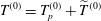 $T^{(0)}=T_{p}^{(0)}+\widetilde{T}^{(0)}$
, then multiplying out and swapping the order of summation and integration, this becomes
 $$\begin{eqnarray}\displaystyle I_{3} & = & \displaystyle ha_{0}^{(0)}\left[P^{(0)}\left(\frac{5}{24}h^{4}+\frac{1}{2}a_{0}^{(0)}h^{3}\right)+b_{0}^{(0)}\right]\int _{0}^{\unicode[STIX]{x1D6FF}}\unicode[STIX]{x1D702}(x)\,\text{d}x\nonumber\\ \displaystyle & & \displaystyle +\,\left[P^{(0)}\left(\frac{5}{24}h^{4}+\frac{1}{2}a_{0}^{(0)}h^{3}\right)+b_{0}^{(0)}\right]\mathop{\sum }_{n}ha_{n}^{(0)}\int _{0}^{\unicode[STIX]{x1D6FF}}\unicode[STIX]{x1D702}(x)\cos (k_{n}x)\,\text{d}x\nonumber\\ \displaystyle & & \displaystyle +\,ha_{0}^{(0)}\mathop{\sum }_{n\geqslant 1}\left(\frac{h^{2}}{2k_{n}}P^{(0)}a_{n}^{(0)}\tanh (k_{n}h)+b_{n}^{(0)}\right)\int _{0}^{\unicode[STIX]{x1D6FF}}\unicode[STIX]{x1D702}(x)\cos (k_{n}x)\,\text{d}x\nonumber\\ \displaystyle & & \displaystyle +\,\mathop{\sum }_{n\geqslant 1}\mathop{\sum }_{m\geqslant 1}ha_{m}^{(0)}\left(\frac{h^{2}}{2k_{n}}P^{(0)}a_{n}^{(0)}\tanh (k_{n}h)+b_{n}^{(0)}\right)\int _{0}^{\unicode[STIX]{x1D6FF}}\unicode[STIX]{x1D702}(x)\cos (k_{n}x)\cos (k_{m}x)\,\text{d}x.\nonumber\\ \displaystyle & & \displaystyle\end{eqnarray}$$
Each integral can be calculated using integration by parts. To solve for the unknown,
 $b_{0}^{(1)}$
, notice that it only appears in the last term of
 $I_{1}$
, and so
 $I_{1}+I_{2}+I_{3}=0$
is easily rearranged to give
 $$\begin{eqnarray}\displaystyle -Q^{(0)}b_{0}^{(1)} & = & \displaystyle P^{(1)}\left(\frac{13}{840}h^{7}+\frac{13}{120}a_{0}^{(0)}h^{6}+\frac{1}{6}(a_{0}^{(0)})^{2}h^{5}\right)+P^{(0)}a_{0}^{(1)}\left(\frac{13}{120}h^{6}+\frac{1}{3}a_{0}^{(0)}h^{5}\right)\nonumber\\ \displaystyle & & \displaystyle +\,\frac{2}{3}\unicode[STIX]{x1D6FF}^{3}ha_{0}^{(0)}\left[P^{(0)}\left(\frac{5}{24}h^{4}+\frac{1}{2}a_{0}^{(0)}h^{3}\right)+b_{0}^{(0)}\right]\nonumber\\ \displaystyle & & \displaystyle +\,\mathop{\sum }_{n\geqslant 1}\left\{\frac{h^{2}a_{n}^{(0)}}{16k_{n}^{3}}(2P^{(0)}a_{n}^{(1)}+P^{(1)}a_{n}^{(0)})\left[k_{n}h(2-\text{sech}^{2}(k_{n}h))-\tanh (k_{n}h)\right]\right.\nonumber\\ \displaystyle & & \displaystyle +\,\frac{1}{2}h(a_{n}^{(0)}b_{n}^{(1)}+a_{n}^{(1)}b_{n}^{(0)})\left(\frac{1}{2}h\,\text{sech}^{2}(k_{n}h)+\frac{1}{2k_{n}}\tanh (k_{n}h)\right)\nonumber\\ \displaystyle & & \displaystyle +\,\left\{ha_{n}^{(0)}\left[P^{(0)}\left(\frac{5}{24}h^{4}+\frac{1}{2}a_{0}^{(0)}h^{3}\right)+b_{0}^{(0)}\right]\right.\nonumber\\ \displaystyle & & \displaystyle +\,\left.\left.ha_{0}^{(0)}\left[\frac{h^{2}}{2k_{n}}P^{(0)}a_{n}^{(0)}\tanh (k_{n}h)+b_{n}^{(0)}\right]\right\}\left(-\frac{2\unicode[STIX]{x1D6FF}}{k_{n}^{2}}\cos (k_{n}\unicode[STIX]{x1D6FF})+\frac{2}{k_{n}^{3}}\sin (k_{n}\unicode[STIX]{x1D6FF})\right)\right\}\nonumber\\ \displaystyle & & \displaystyle +\,\mathop{\sum }_{m\geqslant 1}\mathop{\sum }_{n\geqslant 1}h\left(\frac{h^{2}}{2k_{n}}P^{(0)}a_{m}^{(0)}\tanh (k_{m}h)+b_{m}^{(0)}\right)\tilde{\unicode[STIX]{x1D613}}_{mn}a_{n}^{(0)}\nonumber\\ \displaystyle & & \displaystyle +\,Q_{1}^{(1)}b_{0}^{(0)}.\end{eqnarray}$$