





1. Introduction
Flows of thin films of viscous fluid spreading under the action of gravity are ubiquitous in the world around us, as seen in various industrial (Oron, Davis & Bankoff Reference Oron, Davis and Bankoff1997), environmental (Simpson Reference Simpson1982) and geophysical (Huppert Reference Huppert2006) applications. These range from the spread of oil on the sea (Hoult Reference Hoult1972) to the dynamics of lava flows (Griffiths Reference Griffiths2000), for example. Particularly striking is the range of possible behaviours when a thin film of viscous fluid spreads under gravity over a soft-bedded, or liquid-infused, substrate. Small-scale industrial applications of such lubricated flows include multi-layer thin-film coating processes, such as for electronics and medical devices (Ying et al. Reference Ying, Shi, Wu, Zhang and Wang2015), and three-dimensional printing or additive manufacturing applications (Mukherjee et al. Reference Mukherjee, Zuback, De and DebRoy2016; Sames et al. Reference Sames, List, Pannala, Dehoff and Babu2016), for example. In the latter context, molten material (liquid) is continually added to soft, solidifying substrates that are partially solid and partially liquid, and hence deformable (Khairallah et al. Reference Khairallah, Anderson, Rubenchik and King2016; Kowal, Davis & Voorhees Reference Kowal, Davis and Voorhees2018).
Other examples on the small scale include physiological applications, such as that of nasal drug and vaccine delivery, in which an intranasally delivered liquid drug solution or vaccine interacts with a viscous layer of mucus (Masiuk, Kadakia & Wang Reference Masiuk, Kadakia and Wang2016). A poor understanding of drug–mucus interactions currently hinders the development of effective nasally delivered vaccines, despite their potential to boost effectiveness by targeting respiratory viruses at the point of entry into the body (Madhavan et al. Reference Madhavan2022). A recent clinical trial prompted the need for research to help such vaccines remain in the nose and to reliably quantify the proportion of the drug or vaccine that is cleared away down the nasal passages towards the pharynx and gastrointestinal tract by mucociliary clearance (Masiuk et al. Reference Masiuk, Kadakia and Wang2016; Madhavan et al. Reference Madhavan2022).
On much larger scales, flows of lubricated viscous fluids are relevant to a range of geophysical applications such as the flow of ice sheets (Schoof & Hewitt Reference Schoof and Hewitt2013), which flow over a layer of unconsolidated, water-saturated subglacial sediment, or till. Till is known to act as a basal lubricant for the flow of the overlying ice. It has also been found to accelerate the flow of ice, noticeably flattening its upper surface (Kowal & Worster Reference Kowal and Worster2015). Viscous coupling between ice and till has also been postulated as a possible cause of the formation of fast-flowing ice streams, as observed experimentally (Kumar et al. Reference Kumar, Zuri, Kogan, Gottlieb and Sayag2021; Gyllenberg & Sayag Reference Gyllenberg and Sayag2022). This complements other ice-stream formation mechanisms, including positive feedback between sliding and basal melt production (Fowler & Johnson Reference Fowler and Johnson1995; Sayag & Tziperman Reference Sayag and Tziperman2008), a triple-valued sliding law (Sayag & Tziperman Reference Sayag and Tziperman2009; Kyrke-Smith, Katz & Fowler Reference Kyrke-Smith, Katz and Fowler2014), and thermo-viscous fingering (Payne & Dongelmans Reference Payne and Dongelmans1997; Hindmarsh Reference Hindmarsh2004, Reference Hindmarsh2006). Subglacial till has also been found to accumulate in the grounding zones of ice sheets as observed seismically (Alley et al. Reference Alley, Blankenship, Bentley and Rooney1987; Batchelor & Dowdeswell Reference Batchelor and Dowdeswell2015) and in fluid-mechanical experiments (Kowal & Worster Reference Kowal and Worster2020).
Other geophysical applications of such two-layer flows include magma or lava flows in which a layer of molten material propagates over a solidifying solid–liquid substrate of higher viscosity (Griffiths Reference Griffiths2000), two-layer flows resulting from the interaction of dissimilar magmas (Snyder & Tait Reference Snyder and Tait1995, Reference Snyder and Tait1998), ejecta flows of impact craters (Xiao & Komatsu Reference Xiao and Komatsu2013), and flows in which molten material solidifies by cooling from above (Balmforth & Craster Reference Balmforth and Craster2000). Layered flows in porous media are another example (Woods & Mason Reference Woods and Mason2000), though notably, viscous coupling between the layers – of relevance to the present paper – is absent in a porous medium.
Theoretical and experimental investigations of viscous gravity currents to date include single-layer (Smith Reference Smith1969; Huppert Reference Huppert1982a,Reference Huppertb) and two-layer (Kowal & Worster Reference Kowal and Worster2015; Dauck et al. Reference Dauck, Box, Gell, Neufeld and Lister2019; Shah, Pegler & Minchew Reference Shah, Pegler and Minchew2021) flows over horizontal and inclined substrates, intrusions at the interface between two dissimilar fluids (Lister & Kerr Reference Lister and Kerr1989), flows over curved surfaces (Takagi & Huppert Reference Takagi and Huppert2010) and topological features (Hinton & Hogg Reference Hinton and Hogg2022), and thin-film flows of non-Newtonian viscous fluids (Hewitt & Balmforth Reference Hewitt and Balmforth2013; Hinton Reference Hinton2022; Christy & Hinton Reference Christy and Hinton2023), to name a few. Such flows are often modelled by applying the principles of lubrication theory, which is valid when the fluid layers are long and thin, and similarity solutions often exist in these situations. For example, the frontal position of a viscous gravity current spreading over a horizontal substrate, fed at constant source flux, propagates as  $t^{4/5}$ and
 $t^{1/2}$ in two-dimensional and axisymmetric geometries, respectively (Huppert Reference Huppert1982b). These scalings are also respected for two-layer viscous gravity currents (Kowal & Worster Reference Kowal and Worster2015; Dauck et al. Reference Dauck, Box, Gell, Neufeld and Lister2019), including when modified by a power-law rheology (Leung & Kowal Reference Leung and Kowal2022a). Frequently, such similarity solutions serve as global attractors, which other solutions approach at late times, despite the variety of possible initial conditions (Ball & Huppert Reference Ball and Huppert2019). These similarity solutions have been proven to be stable to small perturbations for single-layer viscous gravity currents propagating over horizontal substrates and for gravity-driven flows in porous media (Mathunjwa & Hogg Reference Mathunjwa and Hogg2006a,Reference Mathunjwa and Hoggb), for example.
A perhaps unexpected feature of some similarity solutions is that in certain configurations, the associated flows may exhibit symmetry-breaking instabilities, similar to viscous fingering instabilities. In particular, we demonstrate in a companion paper (Yang & Kowal Reference Yang and Kowal2024), that viscous gravity currents intruding into another thin film of viscous fluid are susceptible to a novel frontal viscous fingering instability. The instability is similar to the Saffman–Taylor instability for viscous fluids intruding into one another in a Hele-Shaw cell or other porous medium, but this time without a Hele-Shaw cell or any porous medium present.
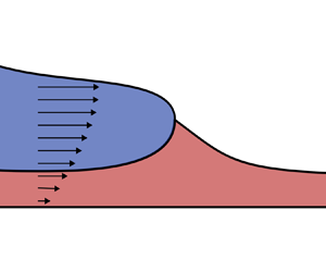
We examine the base flow susceptible to this instability in the present paper. In particular, we examine the flow of a viscous gravity current spreading under its own weight over a horizontal substrate that is pre-wetted by another thin film of viscous fluid of different density and viscosity, as depicted in figure 1. We assume that the flow of both layers is resisted dominantly by vertical viscous shear stresses, and that the effects of inertia and surface tension are negligible. In particular, we apply principles of lubrication theory to model the flow in terms of depth-integrated quantities, and examine similarity solutions describing the flow.
Schematic of a thin film of viscous fluid spreading under gravity over a rigid horizontal substrate pre-wetted by another viscous fluid in an axisymmetric geometry.

We extend the work of Dauck et al. (Reference Dauck, Box, Gell, Neufeld and Lister2019), in which a version of this problem was examined theoretically and experimentally, focusing on the limit in which the two layers are of equal density. This problem is also relevant to the work of Lister & Kerr (Reference Lister and Kerr1989) on the propagation of viscous gravity currents at the interface between two dissimilar fluids. Setting the properties of the uppermost fluid to match that of vapour recovers the present set-up under some additional assumptions made by Lister & Kerr (Reference Lister and Kerr1989), which we remove. These include setting up a quasi-steady equilibrium in which there is no net flux of lower fluid through any cross-section of the flow, and assuming that the intruding fluid is of uniform velocity, which is applicable when the viscosity of the intruding fluid is not much smaller than that of the ambient fluids. We find that a number of our results are recoverable under these assumptions. Other two-layer flows most relevant to our work include those of Kowal & Worster (Reference Kowal and Worster2015), in which the intruding fluid is supplied from below rather than from above, its generalisation to power-law fluids (Gyllenberg & Sayag Reference Gyllenberg and Sayag2022; Leung & Kowal Reference Leung and Kowal2022a), and related two-layer flows down an inclined plane (Shah et al. Reference Shah, Pegler and Minchew2021).
We begin with a theoretical development, deriving the governing equations and similarity solutions in two-dimensional and axisymmetric geometries in § 2. We also characterise a frontal singularity by performing an asymptotic analysis near the nose of the intruding layer in both geometries. We use our similarity solutions in the two geometries to map out the range of different flow behaviours in § 3, discussing changes in the flow regimes as parameters vary, and some asymptotic limits. Finally, we present concluding remarks in § 4.
2. Theoretical development
Consider the flow of two thin films of incompressible, Newtonian viscous fluids of viscosities  $\mu _u$ and
 $\mu _l$, and densities
 $\rho _u$ and
 $\rho _l$, in the configuration depicted in the schematic of figure 1. The subscripts
 $u$ and
 $l$ correspond to quantities involving the upper and lower layers, respectively. The plane
 $z=0$ denotes a rigid, horizontal substrate that has been initially pre-wetted with a uniform depth
 $h_\infty$ of lower-layer fluid. The thicknesses of the upper and lower layers are denoted by
 $H(\boldsymbol {x},t)$ and
 $h(\boldsymbol {x},t)$, respectively, where
 $\boldsymbol {x}$ is the spatial variable:
 $\boldsymbol {x} = (r,\theta,z)$ or
 $(x,y,z)$ in the axisymmetric and two-dimensional geometries, respectively.
Although the flow is depicted in an axisymmetric geometry in figure 1, we consider both axisymmetric and two-dimensional geometries in this work. In the axisymmetric geometry, the two fluids are supplied from a point source at the origin, while in the two-dimensional geometry, the fluids are instead supplied from a line source at  $x=0$. The upper viscous fluid occupies a region from the source up to the intrusion front, denoted by
 $r=r_N(t)$ in the axisymmetric geometry, and
 $x=x_N(t)$ in the two-dimensional geometry. The intrusion front is a moving boundary that splits the domain into two regions: a two-layer region, involving both viscous fluids (
 $0< r< r_N(t)$ and
 $0< x< x_N(t)$ in the axisymmetric and two-dimensional geometries, respectively), and a single-layer region (
 $r>r_N(t)$ and
 $x>x_N(t)$ in the axisymmetric and two-dimensional geometries, respectively) of the same material properties as the lower-layer fluid.
In developing a theoretical framework, we assume that the effects of inertia are negligible, giving rise to a balance of viscous and buoyancy forces, and assume that surface tension and the effects of mixing at the interface between the two fluids are negligible (Huppert Reference Huppert1982b). We also assume that the horizontal length scale associated with the two films of viscous fluid is much greater than the corresponding vertical length scale, and that vertical shear provides the dominant resistance to the flow. We therefore apply the approximations of lubrication theory, and obtain the momentum equations
 \begin{equation} \boldsymbol{0}={-}\boldsymbol{\nabla} p_i +\rho_i\boldsymbol{g} + \mu_i\, \frac{\partial^2\boldsymbol{u}_i}{\partial z^2},\end{equation}
where  $\boldsymbol {u}_i = \boldsymbol {u}_i(\boldsymbol {x},t)$ is the velocity, assumed to be horizontal, the subscript
 $i=u,l$ denotes the upper and lower layers, respectively,
 $\boldsymbol {g}=-g\boldsymbol {e}_z$ is the acceleration due to gravity, and
 $\boldsymbol {e}_z$ is the unit basis vector in the
 $z$-direction.
Our approach is in line with generalised frameworks for two-layer thin film flows (e.g. Gyllenberg & Sayag Reference Gyllenberg and Sayag2022; Christy & Hinton Reference Christy and Hinton2023) and the related work of Dauck et al. (Reference Dauck, Box, Gell, Neufeld and Lister2019). The latter presented generalised equations for a variation of the problem studied here, later focusing on the limit in which  $\rho _u=\rho _l$. Here, we explore flows for which
 $\rho _u\neq \rho _l$, and investigate additional buoyancy effects present in this scenario, which, in particular, change the behaviour of the flow near the intrusion front. We note that the equal density limit is a singular limit in which the order of the equations reduces by one, giving rise to shock-front solutions. These no longer appear when the densities are unequal.
In what follows, we obtain depth-integrated governing equations modelling the flow in axisymmetric and two-dimensional geometries simultaneously. The main difference between the two geometries is the orientation of vectors, such as the velocity vector  $\boldsymbol {u}_i$. These vectors are aligned with the radial and
 $x$-directions in the axisymmetric and two-dimensional geometries, respectively. We organise the main governing equations by the relevant regions: the two-layer region and the single-layer region.
2.1. The two-layer region
Given that vertical shear stresses provide the dominant resistance to the flow, the pressure in the two layers is hydrostatic, so that
 \begin{gather} p_u = \rho_u g (H + h - z), \end{gather}
 \begin{gather}p_l = \rho_u g H + \rho_l g (h-z) \end{gather}
(see e.g. Kowal & Worster Reference Kowal and Worster2015). We assume the upper layer is stress-free at its upper surface, so that
 \begin{equation} \mu_u\,{\frac{\partial{\boldsymbol{u}_u}}{\partial{z}}}=0\quad \mathrm{at}\ z = H+h.\end{equation}
We assume that the velocity and shear stress at the interface between the upper and lower fluids are continuous, so that
 \begin{gather} \boldsymbol{u}_l = \boldsymbol{u}_u \quad \mathrm{at}\ z = h, \end{gather}
 \begin{gather}\mu_l\,{\frac{\partial{\boldsymbol{u}_l}}{\partial{z}}} = \mu_u\,{\frac{\partial{\boldsymbol{u}_u}}{\partial{z}}} \quad \mathrm{at}\ z = h. \end{gather}
We also assume that the lower layer satisfies the no-slip condition at the substrate, so that
 \begin{equation} \boldsymbol{u}_l = 0 \quad \mathrm{at}\ z = 0.\end{equation}
Solving (2.1) for the velocity field subject to (2.4)–(2.7) gives
 \begin{gather} \boldsymbol{u}_u= \left(\frac{(h-z) (h+2 H-z)}{2 \mu _u}-\frac{h H}{\mu _l}\right) \boldsymbol{\nabla} p_u-\frac{h^2}{2 \mu _l}\,\boldsymbol{\nabla} p_l, \end{gather}
 \begin{gather}\boldsymbol{u}_l={-}\frac{H z }{\mu _l}\,\boldsymbol{\nabla} p_u+\frac{z (z-2 h)}{2 \mu _l}\,\boldsymbol{\nabla} p_l. \end{gather}
Integrating these velocities across the depth of each layer yields the depth-integrated flux of upper- and lower-layer fluids, per unit width, given by
 \begin{gather} \boldsymbol{q}_u ={-}\frac{\rho_ug}{3\mu_l}\left[\left(\mathcal{M}H^3+\frac{3}{2}\,H h^2+3H^2 h\right) (\boldsymbol{\nabla} H+\boldsymbol{\nabla} h)+\frac{3}{2}\,\mathcal{D} H h^2\,\boldsymbol{\nabla} h\right], \end{gather}
 \begin{gather}\boldsymbol{q}_l ={-}\frac{\rho_ug}{3\mu_l}\left[\left(\frac{3}{2}\,H h^2+h^3\right) (\boldsymbol{\nabla} H+\boldsymbol{\nabla}h)+\mathcal{D}h^3\,\boldsymbol{\nabla} h\right]. \end{gather}
These align with the relevant expressions presented in Kowal & Worster (Reference Kowal and Worster2015) and Dauck et al. (Reference Dauck, Box, Gell, Neufeld and Lister2019) in two-dimensional and axisymmetric configurations. Here, the dimensionless parameters
 \begin{gather} \mathcal{M} = \frac{\mu_l}{\mu_u}, \end{gather}
 \begin{gather}\mathcal{D} = \frac{\rho_l-\rho_u}{\rho_u}, \end{gather}
define the viscosity ratio and relative density difference, respectively.
The upper surface and the interface between the two fluids evolve in line with the mass conservation equations
 \begin{gather} \frac{\partial H}{\partial t} + \boldsymbol{\nabla}\boldsymbol{\cdot}\boldsymbol{q}_u = 0, \end{gather}
 \begin{gather}\frac{\partial h}{\partial t} + \boldsymbol{\nabla}\boldsymbol{\cdot}\boldsymbol{q}_l = 0, \end{gather}
for the upper and lower layers, respectively. These equations, along with (2.10)–(2.11) for the depth-integrated fluxes, fully specify the evolution of the two free surfaces, subject to appropriate boundary conditions, which we discuss in §§ 2.3 and 2.4.
2.2. The single-layer region
In the single-layer region, we retain the subscript  $l$ to reflect that the material properties are the same as that of the lower layer upstream of the intrusion front. Similarly to the two-layer region, the pressure is hydrostatic in the single-layer region, so that
 \begin{equation} p_l = \rho_l g (h-z) \end{equation}
(see Huppert Reference Huppert1982b). The upper surface satisfies the stress-free condition
 \begin{equation} \mu_l\,{\frac{\partial{\boldsymbol{u}_l}}{\partial{z}}}=0 \quad \mathrm{at}\ z = h,\end{equation}
and we assume the no-slip condition at the substrate,
 \begin{equation} \boldsymbol{u}_l = 0 \quad \mathrm{at}\ z = 0.\end{equation}
Solving (2.1) subject to (2.17) and (2.18) for the velocity profile, and integrating across the depth of the current, gives rise to the depth-integrated flux
 \begin{equation} \boldsymbol{q}_l ={-}\frac{\rho_ug }{3\mu_l}\,(\mathcal{D}+1)h^3\,\boldsymbol{\nabla} h,\end{equation}
in line with Huppert (Reference Huppert1982b). This is supplemented by the mass conservation equation
 \begin{equation} \frac{\partial h}{\partial t} + \boldsymbol{\nabla}\boldsymbol{\cdot}\boldsymbol{q}_l = 0,\end{equation}
which determines the evolution of the free surface. What remains to be done to close the problem is to specify the remaining boundary conditions and matching conditions to couple the two regions, which we organise by geometry.
2.3. Axisymmetric currents
In the axisymmetric geometry, the upper and lower layers flow radially outwards so that  $\boldsymbol {q}_u=q_{u} \boldsymbol {e}_r$ and
 $\boldsymbol {q}_l=q_{l} \boldsymbol {e}_r$, where
 $\boldsymbol {e}_r$ is the radial unit basis vector. We outline the corresponding boundary conditions and matching conditions across the intrusion front below.
Following Kowal & Worster (Reference Kowal and Worster2015), we assume that the upper and lower layers are supplied at a constant source flux  $\hat {\mathcal {Q}}_u$ and
 $\hat {\mathcal {Q}}_l$, respectively, at the origin, so that
 \begin{gather} \lim_{r\rightarrow 0} 2 {\rm \pi}r q_u = \hat{\mathcal{Q}}_u, \end{gather}
 \begin{gather}\lim_{r\rightarrow 0} 2 {\rm \pi}r q_l = \hat{\mathcal{Q}}_l. \end{gather}
The thickness and the flux of the lower layer are continuous across the intrusion front  $r = r_N(t)$, so that
 \begin{gather}{}[h]^+_-= 0\quad \mathrm{at}\ r=r_N, \end{gather}
 \begin{gather}{}[q_l]^+_-= 0\quad \mathrm{at}\ r=r_N. \end{gather}
In addition, the upper-layer flux vanishes at the front, so that
 \begin{equation} q_u = 0\quad \mathrm{at}\ r=r_N.\end{equation}
The front evolves kinematically, which gives rise to an evolution equation for the frontal position,
 \begin{equation} \frac{{\rm d} r_N}{{\rm d} t} =\lim_{r\rightarrow r_N^-}\frac{q_u}{H},\end{equation}
as in Kowal & Worster (Reference Kowal and Worster2015, Reference Kowal and Worster2019a,Reference Kowal and Worsterb) and Gyllenberg & Sayag (Reference Gyllenberg and Sayag2022), for example. In the far field, we approach a uniform thickness, so that
 \begin{equation} \lim_{r\rightarrow \infty}h =h_\infty.\end{equation}
This condition implies that the flux vanishes in the far field.
The boundary conditions and matching conditions specified in this section fully close the problem for the evolution of the two liquid layers. This includes the frontal position, which needs to be determined as part of the solution of the problem.
2.3.1. Self-similar axisymmetric flows
Although there is an externally imposed vertical length scale  $h_{\infty }$, the lack of a horizontal length scale is sufficient to allow for the existence of a similarity solution, which we can also deduce by performing a scaling analysis. In the axisymmetric geometry, such similarity solutions exist only when the source flux is constant, as assumed here. However, as discussed in § 2.4.1, similarity solutions do not exist if the source flux is constant in the two-dimensional geometry. Instead, it is necessary for the source flux to follow a specific power law, proportional to
 $t^a$ for some constant
 $a$, in order for similarity solutions to exist in two dimensions. For a related problem in which a viscous gravity current intrudes at the interface between two dissimilar fluids, it has been reported that in either geometry, the late-time behaviour of the injected fluid depends crucially on
 $a$ (Lister & Kerr Reference Lister and Kerr1989). Below a critical value, the injected fluid reduces in height with time, allowing us to approximate the lower fluid layer to be uniform in height. Above the critical value, the injected fluid height increases with time, allowing the effects of the lower fluid to be neglected, thus recovering the classical single-layer gravity current. At the critical value, the injected fluid height is constant in time, and exact similarity solutions exist (Lister & Kerr Reference Lister and Kerr1989).
Formally, solutions obtained from specific initial conditions approach a similarity solution at late times for diffusive problems of the type considered here (Ball & Huppert Reference Ball and Huppert2019). This is seen also in analogue laboratory experiments, in which flows become self-similar after an initial transient (Huppert Reference Huppert1982b).
To formulate the governing equations in terms of similarity variables, and to non-dimensionalise the problem, we introduce the changes of variables
 \begin{equation} (\xi,\xi_N) = \left(\frac{Qt}{2{\rm \pi} h_{\infty}}\right)^{{-}1/2}(r, r_N ) = (2{\rm \pi})^{3/8}\left(\frac{\rho_ugQ^3}{3\mu_l}\right)^{-{1}/{8}} t^{-{1}/{2}}(r,r_N) \end{equation}
for the spatial variable and the frontal position,
 \begin{equation} (F(\xi),f(\xi))=\frac{1}{h_{\infty}}\,(H(r,t),h(r,t)) =(2{\rm \pi})^{1/4}\left(\frac{\rho_ug}{3\mu_lQ}\right)^{{1}/{4}}(H(r,t),h(r,t)),\end{equation}
for the thicknesses, and
 \begin{equation} (\phi_u(\xi),\phi_l(\xi))=\sqrt{\frac{2 {\rm \pi}t}{h_{\infty} Q}}\,(q_u(r,t),q_l(r,t)) = \left(\frac{(2{\rm \pi})^5\rho_ugt^4}{3\mu_lQ^5}\right)^{{1}/{8}}(q_u(r,t),q_l(r,t)) \end{equation}
for the flux of both layers. Here, we define
 \begin{equation} Q =2{\rm \pi} h_{\infty}^4\,\frac{\rho_u g}{3\mu_l} \end{equation}
to be a dimensional measure of the flux associated with depth  $h_\infty$. Using this measure, we non-dimensionalise the source fluxes as
 \begin{equation} (\mathcal{Q}_u,\mathcal{Q}_l) = Q^{{-}1} (\hat{\mathcal{Q}}_u,\hat{\mathcal{Q}}_l). \end{equation}
Substituting into the governing equations (2.14)–(2.15) and (2.20), describing mass conservation, yields the ordinary differential equations
 \begin{gather} -\frac{1}{2}\,F'\xi + \frac{1}{\xi}\,(\xi \phi_u)'=0, \end{gather}
 \begin{gather}-\frac{1}{2}\,f'\xi + \frac{1}{\xi}\,(\xi \phi_l)'=0, \end{gather}
where the radial components of the fluxes of fluid within the two layers, in both regions of the domain, are given by
 \begin{equation} \phi_u = \begin{cases} -\left[\left(\mathcal{M}F^3+\tfrac{3}{2}F f^2+3F^2 f\right)(F'+ f')+ \tfrac{3}{2}\mathcal{D} F f^2 f'\right], & 0<\xi<\xi_N,\\ 0, & \xi\ge\xi_N, \end{cases} \end{equation}
and
 \begin{equation} \phi_l = \begin{cases} -\left[\left(\tfrac{3}{2}Ff^2+f^3\right)( F'+ f' )+\mathcal{D}f^3 f'\right], & 0< \xi<\xi_N,\\ -(\mathcal{D}+1)f^3 f', & \xi\ge\xi_N. \end{cases} \end{equation}
These are obtained from (2.10)–(2.11) and (2.19). Here, the prime  $'$ denotes differentiation with respect to
 $\xi$. These equations are supplemented by the boundary conditions
 \begin{gather} \xi \phi_u \rightarrow \mathcal{Q}_u,\quad \xi \phi_l \rightarrow \mathcal{Q}_l\quad \text{as}\ \xi \rightarrow 0^+, \end{gather}
 \begin{gather}{}[f]^+_-= 0,\quad [\phi_l]^+_-= 0,\quad \phi_u= 0\quad \text{at}\ \xi = \xi_N, \end{gather}
 \begin{gather}\frac{\phi_u}{F} \rightarrow\frac{1}{2}\,\xi_N\quad \text{as}\ \xi\rightarrow\xi_N^-, \end{gather}
 \begin{gather}f \rightarrow 1\quad \text{as}\ \xi\rightarrow \infty, \end{gather}
at the source, at the intrusion front, and in the far field, all derived from the dimensional boundary conditions (2.21)–(2.27). This system of differential equations and corresponding boundary conditions and matching conditions fully prescribes the evolution of the two layers in similarity coordinates. These equations were solved using a shooting method implemented using Mathematica's in-built solver NDSolve. The governing equations were integrated outwards from the front on a finite domain. Instead of subtracting the singularities at  $\xi =0$ and
 $\xi =\xi _N$ analytically, the domain was truncated to avoid the singular points, and auxiliary boundary conditions using the asymptotic solution of § 2.3.2 were implemented. Numerical results are discussed in subsequent subsections.
2.3.2. Asymptotic solutions near the nose of axisymmetric intrusions
Near the intrusion front  $\xi =\xi _N$, the normal component of the upper-layer flux
 $\phi _u$ and the upper-layer thickness
 $F$ tend to 0, while thickness gradients and stress diverge. A similar stress singularity features at the intrusion front of single-layer (Huppert Reference Huppert1982b) and two-layer (Kowal & Worster Reference Kowal and Worster2015, Reference Kowal and Worster2019b; Gyllenberg & Sayag Reference Gyllenberg and Sayag2022; Leung & Kowal Reference Leung and Kowal2022a,Reference Leung and Kowalb) viscous gravity currents under the approximations of lubrication theory.
We examine the singular point  $\xi =\xi _N$ asymptotically by performing a local analysis following the approach of Huppert (Reference Huppert1982b), Kowal & Worster (Reference Kowal and Worster2015) and Leung & Kowal (Reference Leung and Kowal2022a). As shown in Appendix A, we obtain asymptotic solutions that feature a square-root singularity of the form
 \begin{gather} F \sim A_1\delta^{{1}/{2}}+A_2\delta+\cdots, \end{gather}
 \begin{gather}f \sim a_0+a_1\delta^{{1}/{2}}+a_2\delta+\cdots, \end{gather}
valid for  $\delta = (1-{\xi }/{\xi _N})\ll 1$. Equations (A3) and (A10)–(A11) in Appendix A demonstrate that the coefficients
 $a_1$,
 $A_2$ and
 $a_2$ of the higher-order terms can be written in terms of
 $A_1$,
 $a_0$ and
 $\xi _N$. The latter set of coefficients can be determined by matching to the outer numerical solutions. This square-root singularity is also observed by Lister & Kerr (Reference Lister and Kerr1989) in a similar scenario involving a thin current moving over a nearly uniform lower layer, and by Dauck et al. (Reference Dauck, Box, Gell, Neufeld and Lister2019) in the equal-density limit. The asymptotic solution identified by Lister & Kerr (Reference Lister and Kerr1989) in this scenario is in agreement with (2.41)–(2.42) if we set
 $\mathcal {Q}_l=0$ to account for the lower layer remaining uniform.
The asymptotic approximations (2.41)–(2.42) elucidate the behaviour near the front, and inform an appropriate scheme for the numerical solution of the full system of governing differential equations. These asymptotic solutions are shown in figure 2(a) up to  $\textit {O}(\delta ^{1/2})$ and
 $\textit {O}(\delta )$, in comparison to the full numerical solutions, which are valid throughout the domain. As expected, the more terms we include in the asymptotic expansion, the better the agreement with the full numerical solution near the front, as can be seen by including terms up to
 $\textit {O}(\delta )$ versus terms up to
 $\textit {O}(\delta ^{1/2})$. Our asymptotic calculation also indicates that the upper-layer pressure gradient
 $F'+f'$ is singular at the front, while the lower-layer pressure gradient
 $F'+(1+\mathcal {D}) f'$ is non-singular.
The full numerical solution versus the asymptotic solutions (2.41)–(2.42) near the intrusion front in (a) axisymmetric and (b) two-dimensional geometries, for  $\mathcal {M}=0.1$,
 $\mathcal {D}=0.3$,
 $\mathcal {Q}_u = 1$ and
 $\mathcal {Q}_l=0.5$. Solid curves indicate the full numerical solution. Dotted curves indicate the asymptotic solution containing terms up to
 $O(\delta ^{1/2})$. Dashed curves indicate the asymptotic solution containing terms up to
 $O(\delta )$.

We note that the structure of the frontal singularity at  $\xi =\xi _N$ differs from that of single-layer viscous gravity currents propagating over a rigid horizontal substrate, for which the thickness is
 $\textit {O}(\delta ^{1/3})$ rather than
 $\textit {O}(\delta ^{1/2})$, as
 $\delta \to 0$ (Huppert Reference Huppert1982b). This also contrasts with the structure of the singularity at the front of a thin film of viscous fluid spreading beneath another viscous gravity current, for which the thickness of the intruding layer is also
 $\textit {O}(\delta ^{1/3})$ as
 $\delta \to 0$ (Kowal & Worster Reference Kowal and Worster2015, Reference Kowal and Worster2019a,Reference Kowal and Worsterb).
We include  $\textit {O}(\delta )$ terms in the asymptotic solution (2.41)–(2.42) during the initialisation of the numerical computation, as they play a role in determining the lower-layer flux at the nose. In particular, replacing quantities associated with the lower layer by their asymptotic approximations gives rise to the following leading-order asymptotic expression for the lower-layer flux:
 \begin{equation} \phi_l = \frac{3 a_0^2 A_1^2 \mathcal{D}}{4\xi _N (\mathcal{D}+1)}+ \frac{a_0^3 }{\xi _N}\,A_2+\frac{ a_0^3 (\mathcal{D}+1)}{\xi _N}\,a_2+ \textit{O}(\delta^{{1}/{2}}),\end{equation}
which simplifies to
 \begin{equation} \phi_l = \frac{a_0 \xi _N}{3}-\frac{a_0^2 A_1^2 \mathcal{D}}{4\xi _N (\mathcal{D}+1)}+ \textit{O}(\delta^{{1}/{2}}), \end{equation}
using (A10)–(A11). Importantly, (2.43) shows that the leading-order contribution to  $\phi _l$ includes correction terms involving the second-order coefficients
 $a_2$ and
 $A_2$. The appearance of these coefficients in the leading-order expression for the lower-layer flux emphasises the need to determine them, which is equivalent to determining the
 $\textit {O}(\delta )$ terms in the asymptotic solution (2.41)–(2.42).
2.4. Two-dimensional currents
In the two-dimensional configuration, the upper and lower layers flow in the  $x$-direction so that
 $\boldsymbol {q}_u=q_{u} \boldsymbol {e}_x$ and
 $\boldsymbol {q}_l=q_{l} \boldsymbol {e}_x$, where
 $\boldsymbol {e}_x$ is the unit basis vector in the
 $x$-direction. Below, we specify the associated boundary conditions and matching conditions to couple the two regions of the flow.
For reasons described in § 2.3.1, we assume that the upper and lower layers are supplied at specified line fluxes  ${\hat {\mathcal {Q}}_u}t^a$ and
 ${\hat {\mathcal {Q}}_l}t^a$, respectively, where
 $\hat {\mathcal {Q}}_u$,
 $\hat {\mathcal {Q}}_l$ and
 $a>-1$ are constants. Explicitly,
 \begin{equation} q_u = \hat{\mathcal{Q}}_ut^a,\quad q_l = \hat{\mathcal{Q}}_lt^a \quad \text{at}\quad x=0.\end{equation}
Equivalently, the volume of injected fluid is given by  $\hat {\mathcal {Q}}_ut^{a+1}/(a+1)$ and
 $\hat {\mathcal {Q}}_l t^{a+1}/(a+1)$ for the upper and lower layers, respectively. When
 $-1< a<0$, the two fluids are supplied at a rate that is decreasing with time from a point singularity at
 $t=0$, while the volume is increasing with time. Experimentally, such a flow can be achieved by releasing a finite volume of fluid at
 $t=0$, followed by a time-dependent supply of fluid at the source.
The thickness and the normal flux of the lower layer are assumed to be continuous across the intrusion front  $x = x_N(t)$, so that (2.23)–(2.24) hold but at
 $x=x_N$ rather than at
 $r=r_N$. In addition, the normal component of the upper-layer flux vanishes at the front, so that (2.25) holds but at
 $x=x_N$. The front evolves kinematically, which yields the evolution equation (2.26) for the frontal position, with
 $r_N$ replaced by
 $x_N$. In the far field, the thin film approaches a uniform thickness, so that (2.27) continues to hold. These boundary/matching conditions and the two-dimensional version of the system of differential equations (2.10)–(2.11), (2.14)–(2.15), (2.19)–(2.20) are sufficient to fully specify the evolution of the two-dimensional flow.
2.4.1. Self-similar two-dimensional flows
In contrast to axisymmetric flows, similarity solutions do not exist in the two-dimensional geometry when the flux is constant, as mentioned in § 2.3.1. Instead, a specific power law is required for a similarity solution to exist, consistently with prior work on related problems (Lister & Kerr Reference Lister and Kerr1989; Dauck et al. Reference Dauck, Box, Gell, Neufeld and Lister2019). In particular, the flow becomes self-similar when  $a = -\frac {1}{2}$, as can be seen through a scaling argument. Such similarity solutions serve as attractors, to which other two-dimensional solutions, associated with different initial conditions, converge at late times (Ball & Huppert Reference Ball and Huppert2019). To formulate the governing equations in similarity variables, we introduce the changes of variables
 \begin{equation} (\xi,\xi_N) = \frac{h_{\infty}}{Qt^{1/2}}(x, x_N)= \left(\frac{3\mu_l}{\rho_ugQ^3}\right)^{{1}/{5}} t^{-({1}/{2})}(x,x_N) \end{equation}
for the spatial coordinate and the frontal position,
 \begin{equation} (F(\xi),f(\xi))= \frac{1}{h_{\infty}}\,(H(x,t),h(x,t))= \left(\frac{\rho_ug}{3\mu_lQ^2}\right)^{{1}/{5}}(H(x,t),h(x,t)) \end{equation}
for the thicknesses, and
 \begin{equation} (\phi_u(\xi), \phi_l(\xi))= Q^{{-}1}t^{1/2}(q_u(x,t), q_l(x,t)) \end{equation}
for the fluxes of the two layers. Here, we define
 \begin{equation} Q =\left(\frac{\rho_ug}{3\mu_l}\right)^{{1}/{2}} h_\infty^{{5}/{2}} \end{equation}
to be a dimensional measure of the flux associated with the thickness  $h_\infty$. Using this measure, we express the two constants describing the source fluxes in dimensionless form as
 \begin{equation} (\mathcal{Q}_u,\mathcal{Q}_l) = Q^{{-}1} (\hat{\mathcal{Q}}_u,\hat{\mathcal{Q}}_l). \end{equation}
In similarity coordinates, the governing equations yield the system of ordinary differential equations
 \begin{gather} -\tfrac{1}{2}\,F'\xi + \phi_u'=0, \end{gather}
 \begin{gather}-\tfrac{1}{2}\,f'\xi + \phi_l'=0, \end{gather}
describing conservation of mass within the two layers, where the upper- and lower-layer fluxes in both regions of the domain, upstream and downstream of the intrusion front, are given by the same expressions (2.35)–(2.36) as in the axisymmetric geometry.
As we switch to the two-dimensional geometry, the only boundary conditions that change are the source flux conditions
 $$\begin{gather} \phi_u = \mathcal{Q}_u,\quad \phi_l = \mathcal{Q}_l \quad \text{at}\ \xi = 0. \end{gather}$$
The remaining boundary conditions and matching conditions remain the same. This includes continuity of thickness and flux across the intrusion front (2.37a,b), the kinematic condition for the evolution of the intrusion front (2.39), and the far-field condition (2.40). These governing equations and boundary conditions are sufficient to fully determine the two-dimensional similarity solutions.
2.4.2. Asymptotic solutions near the nose of two-dimensional intrusions
It can be verified that the local analysis of § 2.3.2, including the asymptotic solutions (2.41)–(2.42) and the relationships between  $a_1$,
 $A_2$ and
 $a_2$ and the quantities
 $A_1$,
 $a_0$ and
 $\xi _N$, apply to the two-dimensional geometry without modification. The expansions are identical in the two geometries as the analysis is local to the front, and the governing equations are identical in the two geometries apart from differences in the divergence in flux (factors of
 $\xi$ and
 $1/\xi$), which affects only the asymptotic solution at higher orders. Apart from differences in the divergence in flux, the equations are identical because the similarity scalings reflect a non-constant source flux (proportional to
 $t^{-1/2}$) in the two-dimensional case, and a constant source flux in the axisymmetric case. Had the source fluxes in both geometries been constant, there would have been additional differences in the governing equations, and hence in the asymptotic solutions, between the two geometries. An illustration of this difference includes prior work in which the intruding layer is supplied from below (see e.g. Kowal & Worster Reference Kowal and Worster2015).
A comparison between the asymptotic solutions up to  $\textit {O}(\delta ^{1/2})$ and up to
 $\textit {O}(\delta )$ against the full numerical solutions, valid throughout the whole domain, is shown in figure 2(b) in the two-dimensional geometry. As in the axisymmetric case, it is unsurprising that there is better agreement between the asymptotic solutions and the full numerical solutions near the front, the more terms are included in the asymptotic expansion. In particular, including terms up to
 $\textit {O}(\delta )$ improves the agreement over a wider neighbourhood of the front in comparison to terms up to
 $\textit {O}(\delta ^{1/2})$. The structure of the singularity remains the same as in the axisymmetric geometry; namely, the thickness is
 $\textit {O}(\delta ^{1/2})$ as
 $\delta \to 0$. This contrasts with the structure of the frontal singularity for single-layer viscous gravity currents propagating over a rigid horizontal substrate, and for thin films of viscous fluid intruding beneath another viscous gravity current (Huppert Reference Huppert1982b; Kowal & Worster Reference Kowal and Worster2015, Reference Kowal and Worster2019a,Reference Kowal and Worsterb).
3. Results and discussion
As found in § 2, the flow of thin films of viscous fluid over pre-lubricated substrates depends upon the four dimensionless parameters  $\mathcal {M}$,
 $\mathcal {D}$,
 $\mathcal {Q}_u$ and
 $\mathcal {Q}_l$, yielding a range of different flow regimes. Figure 3 depicts typical similarity solutions for the profile thicknesses of the two layers in axisymmetric and two-dimensional geometries as the viscosity ratio
 $\mathcal {M}$ and fluxes
 $\mathcal {Q}_u$ and
 $\mathcal {Q}_l$ vary, while the flux ratio
 $\mathcal {Q}_l/\mathcal {Q}_u$ remains fixed. The main difference in the profiles between the two geometries is the presence of a logarithmic singularity at the origin, in which the thickness of both layers diverges, for axisymmetric flows. This is a purely geometric effect, arising from the fact that axisymmetric flows are supplied at non-zero flux from a point source. This is also the case for single-layer axisymmetric flows supplied at non-zero flux (Huppert Reference Huppert1982b).
Numerical solutions for the self-similar flow of a thin film of viscous fluid spreading over another thin film of fluid in (a) axisymmetric and (b) two-dimensional geometries for various viscosity ratios  $\mathcal {M}$ and source fluxes
 $\mathcal {Q}_u$ and
 $\mathcal {Q}_l$, such that
 $\mathcal {Q}_u = 5\mathcal {Q}_l= \mathcal {Q}$. The density difference is fixed at
 $\mathcal {D}=1$.

A range of possible flow profiles across parameter space is displayed in figures 3(a,b) for the axisymmetric and two-dimensional geometries, respectively. Relative to the lower layer, the upper layer is thick and of small extent when the viscosity ratio is low and the upper-layer flux is high, as seen in the top-left panels of figures 3(a,b), and thin when the viscosity ratio is high, as seen in the top-right panels. Decreasing the upper-layer flux reduces the thickness and extent of the upper layer, as seen in the bottom-right panels of figures 3(a,b), while decreasing the viscosity ratio further increases the thickness of the upper layer, and reduces its extent, as seen in the bottom-left panels. In general, low-viscosity ratios correspond to thick upper layers, while high viscosity ratios correspond to thin upper layers, which coat the lower layer from above. Such low-viscosity, thin coating films exert negligible traction at the interface between the two fluids, and only negligibly affect the dynamics of the lower layer, save near the front.
There is a change in behaviour of the flow as we traverse from the origin to the nose, in that the contribution  $q_{lb}\equiv -(1+\mathcal {D})f^3f'$ to the lower-layer flux from gravitational spreading under its own weight (associated with lower-layer buoyancy forces) is positive near the source and negative near the front, as can be identified by examining the sign of
 $f'$. In particular, as displayed in the top-left panels of figures 3(a,b), for example, the interface slope
 $f'$ changes sign from negative near the source to positive near the front, hence the opposite sign change occurs for
 $q_{lb}$. This indicates that lower-layer buoyancy forces tend to decrease the outwards flow of the lower layer near the front. These buoyancy forces are relatively more important, over a larger proportion of the domain the more viscous the upper layer (the smaller
 $\mathcal {M}$ is). For very viscous upper layers, the flow is mainly uniform within the upper layer, and the curvature of the interface between the two layers is relatively small over most of the domain, save for a small region in which the slope of the interface between the two layers changes sign, as demonstrated in the top-left panels of figures 3(a,b) and in figure 4. That is, the change in sign of
 $q_{lb}$ is more pronounced, the more viscous the upper layer. This occurs in both axisymmetric and two-dimensional geometries, which precludes geometric effects, arising from the singularity at the origin in the axisymmetric geometry.
Radial velocity profiles in similarity coordinates (in the axisymmetric geometry), integrated over a disc of radius  $\xi$, for (a)
 $\mathcal {M}=0.1$, (b)
 $\mathcal {M}=1$, and (c)
 $\mathcal {M}=10$, where
 $\mathcal {D}=0.5$,
 $\mathcal {Q}_u=0.5$,
 $\mathcal {Q}_l=0.1$.

The flow at low viscosity ratios is equivalent to the upper layer being almost solid and lubricated from below by a much less viscous fluid. Rescaling variables with respect to the upper layer rather than the lower layer reveals an analogy to the plug flow of a thin film of viscous fluid over an inviscid layer. This regime is in some degree relevant to experiments involving the flow of ice shelves floating freely over the ocean, except that here we neglect the resistance of viscous extensional stress or any transverse shear stress, which would be more important than shear stress in nature. Examples include experiments of viscous gravity currents over an inviscid layer in unconfined geometries (Robison, Huppert & Worster Reference Robison, Huppert and Worster2010; Pegler & Worster Reference Pegler and Worster2012) and in a narrow channel (Pegler et al. Reference Pegler, Kowal, Hasenclever and Worster2013; Kowal, Worster & Pegler Reference Kowal, Worster and Pegler2016). Another example involves experiments of the formation of lava deltas in the limit in which the injected fluid is less dense than the ambient inviscid layer (Taylor-West, Balmforth & Hogg Reference Taylor-West, Balmforth and Hogg2024).
Radial velocity profiles of the two thin films are depicted in figure 4 in an axisymmetric geometry for various viscosity ratios. As shown in figure 4(a), the velocity profile is mainly uniform within the upper layer for small viscosity ratios, and most of the shear is confined to the lower layer alone. The flow of the lower layer transitions from a primarily Couette flow, upstream of the intrusion front, to a parabolic Poiseuille flow ahead of the intrusion front. As the viscosity ratio increases, the upper layer thins and its velocity increases, as do the velocity gradients within the upper layer, as shown in figures 4(b,c).
As seen in figure 5, for large enough density differences, the velocity of the lower layer near the intrusion front becomes negative (the flow reverses) near the lower boundary. This reflects the existence of a stagnation line (where the velocity is zero), which intersects the bottom boundary near the front. Similar flow reversals have been reported by Lister & Kerr (Reference Lister and Kerr1989), in the limiting scenario in which the lower layer is shallow, which requires  $\mathcal {Q}_u \ll 1$ and
 $\mathcal {Q}_l = 0$ in our notation. In fact, the velocity profiles of figure 5 approach that of Lister & Kerr (Reference Lister and Kerr1989) (shown in figure 5 as a dashed red curve, from their (2.27)) as
 $\mathcal {D}\to \infty$. Such flow reversals occur above a critical value of the density difference, above which the lower layer spreads mainly under its own weight. In particular, in contrast to single-layer flows, gradients of the lower-layer thickness are positive near the nose, giving rise to negative contributions to the velocity profile, akin to those of blade coating problems. This effect is more pronounced for low viscosity ratios, for which the upper layer is relatively more viscous in comparison to the lower layer and there are greater thickness gradients near the nose. An alternative explanation for this reverse flow near the front can be understood by considering mass conservation. The negative velocity near the substrate counteracts higher velocities near the interface, arising from viscous coupling between the two layers, so as to conserve mass. This is particularly relevant when the density of the lower layer greatly exceeds that of the upper layer (large
 $\mathcal {D}$), in which case the lower-layer thickness gradient and flux become small.
Scaled lower-layer radial velocity near the nose as a function of depth in similarity coordinates in the axisymmetric geometry (solid curves), evaluated at  $\xi =0.99\xi _N$ for varying
 $\mathcal {D}=0.5, 1, 3, 10, 500$ and
 $\mathcal {M}=10$,
 $\mathcal {Q}_u=0.1$,
 $\mathcal {Q}_l=0.001$. The velocity becomes negative near the lower boundary for large enough density differences. These velocity profiles are compared against the lower-layer velocity profile predicted by Lister & Kerr (Reference Lister and Kerr1989), which is valid for
 $\mathcal {Q}_u \ll 1$ and
 $\mathcal {Q}_l = 0$ (dashed red curve).

As seen in the numerical solutions displayed in figure 6, it is interesting to note that the slope of the interface between the two layers steepens as we decrease the density difference towards zero. The smaller the density difference, the steeper the interface near the intrusion front. As the density difference decreases, these solutions approach a shock front in which the thickness of the upper layer is non-zero at the front while the thickness of lower layer is discontinuous. These shock-front solutions arise in the equal-density limit under the approximations of lubrication theory, as described by Dauck et al. (Reference Dauck, Box, Gell, Neufeld and Lister2019), when the viscosity ratio is large enough.
Profile thicknesses (solid curves) in (a) axisymmetric and (b) two-dimensional geometries as the density difference varies, in comparison to the large- $\mathcal {D}$ asymptotic solution (dashed curve). Parameter values used:
 $\mathcal {M}=2$,
 $\mathcal {D}=0.05,0.2,0.5,1, 3,10,100$,
 $\mathcal {Q}_l=0.1$ and
 $\mathcal {Q}_u=0.5$.

On the other hand, as the density difference approaches infinity, the lower layer becomes significantly denser than the upper layer, and the interface between the two layers becomes flat to leading order, as demonstrated through an asymptotic analysis for  $\mathcal {D}\gg 1$, outlined in Appendix B. Asymptotic solutions valid for
 $\mathcal {D}\gg 1$ are overlain in figure 6, depicting a close match to full numerical solutions when
 $\mathcal {D}$ is large. The higher the density difference
 $\mathcal {D}$, the flatter the interface between the two fluids, as depicted in figure 6.
In contrast to changes in the thickness gradients near the nose, the position of the nose varies only minimally as the density difference varies over three orders of magnitude, as shown in figure 7. With the chosen scaling for the similarity variable  $\xi$ as defined in (2.28) for the axisymmetric geometry, and (2.46) for the two-dimensional geometry, this implies that the speed of the upper-layer fluid remains largely unchanged by the density of the lower-layer fluid.
The extent of the intruding layer of fluid as a function of the density difference. The large- $\mathcal {D}$ limit is shown as a dashed curve. Parameter values used:
 $\mathcal {M}=2$,
 $\mathcal {Q}_l=0.1$ and
 $\mathcal {Q}_u=0.5$. Blue indicates axisymmetric flows; black indicates two-dimensional flows.

There are two asymptotic limits corresponding to small and large viscosity ratios  $\mathcal {M}$, as depicted in figures 8 and 9, which display the frontal position
 $\xi _N$ and the average thickness of the upper layer as a function of the viscosity ratio and how these approach different power laws in both limits. We examine these limits by rescaling the dependent variables with respect to the lower (or upper) layer for small (or large) viscosity ratios. For large viscosity ratios (
 $\mu _u\ll \mu _l$), the upper layer is much more mobile, undergoing larger deformations than the lower layer. This gives rise to upper layers that are long and thin, as depicted in the right-hand panels of figures 3(a,b) and in 10. In this limit, the deformation of the lower layer is negligible compared to that of the upper layer, and the nose position can be determined solely by the upper layer. Therefore, we expect the nose position to scale with the horizontal length scale associated with the deformation of the upper layer. That is, it is appropriate to scale the similarity variable
 $\xi$ with respect to quantities describing the properties of the upper layer. This can be done by rescaling the spatial similarity coordinates (2.28) and (2.46) by factors
 $\mathcal {M}^{1/8}$ in the axisymmetric geometry and
 $\mathcal {M}^{1/5}$ in the two-dimensional geometry, and the thicknesses (2.29) and (2.47) by factors
 $\mathcal {M}^{-1/4}$ in the axisymmetric geometry and
 $\mathcal {M}^{-1/5}$ in the two-dimensional geometry. As shown in figure 8, the nose position indeed varies as
 $\mathcal {M}^{1/8}$ and
 $\mathcal {M}^{1/5}$ for
 $\mathcal {M}\gg 1$, in the axisymmetric and two-dimensional geometries, respectively. Similarly, the average thickness of the upper layer indeed scales as
 $\mathcal {M}^{-1/4}$ and
 $\mathcal {M}^{-1/5}$ for
 $\mathcal {M}\gg 1$, in the axisymmetric and two-dimensional geometries, respectively, as shown in figure 9.
The extent of the intruding layer of fluid as a function of the viscosity ratio. Parameter values used:  $\mathcal {D}=2$,
 $\mathcal {Q}_l=0.1$ and
 $\mathcal {Q}_u=0.5$. Blue indicates axisymmetric flows; black indicates two-dimensional flows.

The average thickness of the upper layer as a function of the viscosity ratio. Parameter values used:  $\mathcal {D}=2$,
 $\mathcal {Q}_l=0.1$ and
 $\mathcal {Q}_u=0.5$. Blue indicates axisymmetric flows; black indicates two-dimensional flows.

For small viscosity ratios ( $\mu _u\gg \mu _l$), the upper layer is much less mobile, undergoing much smaller deformations than the lower layer. The upper layer thickness is large relative to the lower layer, and its extent is small, as depicted in the left-hand panels of figures 3(a,b) and in 10 for a range of values of the viscosity ratio. In this limit, the lower layer undergoes significantly greater deformation compared to the upper layer, so the nose position is solely determined by lower-layer dynamics. As such, scaling with respect to quantities describing the properties of the lower layer is appropriate, as in our initial choice of similarity scalings (2.28)–(2.30) and (2.46)–(2.48). Under this choice of scaling, we expect the nose position to approach a constant as the viscosity ratio approaches zero (
 $\mathcal {M}\ll 1$), which is confirmed in figure 8. Similarly, the average upper-layer thickness approaches a constant as the viscosity ratio approaches zero (
 $\mathcal {M}\ll 1$), as depicted in figure 9.
Profile thicknesses in (a) axisymmetric and (b) two-dimensional geometries as the viscosity ratio varies. Parameter values used:  $\mathcal {D}=2$,
 $\mathcal {M}=0, 1, 10, 100$,
 $\mathcal {Q}_l=0.1$ and
 $\mathcal {Q}_u=0.5$.

As illustrated in figure 11 in both geometries, variations in the upper-layer flux  $\mathcal {Q}_u$ lead to two distinct parameter regimes, characterised by whether
 $\mathcal {Q}_u \ll \mathcal {Q}_l \sim \mathcal {Q}_\infty$ or
 $\mathcal {Q}_u \gg \mathcal {Q}_l \sim \mathcal {Q}_\infty$, given a fixed value of
 $\mathcal {Q}_l\sim \mathcal {Q}_\infty$. Here,
 $\mathcal {Q}_\infty$ is a dimensionless measure of flux associated with the depth of the lower layer in the far-field. Although we find it illuminating to refer to
 $\mathcal {Q}_\infty$ explicitly in this discussion, we note that owing to our choice of similarity scalings, we have
 $\mathcal {Q}_\infty =1$. Thickness profiles in both of these parameter regimes are depicted in figure 12 for a range of values of
 $\mathcal {Q}_u$. In the former limit (
 $\mathcal {Q}_u \ll \mathcal {Q}_l \sim \mathcal {Q}_\infty$), the nose position is determined by the dynamics of the lower layer, which is fed at a specified flux determined by
 $\mathcal {Q}_l$, so that
 $\xi _N$ tends towards a constant as
 $\mathcal {Q}_u\to 0$. We examine this limit in more detail in Appendix C, where we arrive at an asymptotic solution for the nose position when
 $\mathcal {Q}_u\ll 1$, which compares well against the full numerical solutions, as shown in figure 11. The upper layer thickness becomes small in this limit, and scales with
 $\mathcal {Q}_u\ll 1$. In the latter limit (
 $\mathcal {Q}_u \gg \mathcal {Q}_l \sim \mathcal {Q}_\infty$), the upper layer is much thicker than the lower layer, as shown in figure 12. The nose position in this limit is determined by the dynamics of the upper layer, for which the effects of the lower layer are negligible. In effect, the dynamics of the upper layer tend towards that of a single-layer viscous gravity current fed at a specified flux determined by
 $\mathcal {Q}_u$ as
 $\mathcal {Q}_u\to \infty$. Therefore, the nose position
 $\xi _N$ scales with the upper-layer flux as
 $\mathcal {Q}_u^{3/5}$ in the two-dimensional geometry, and
 $\mathcal {Q}_u^{3/8}$ in the axisymmetric geometry, as confirmed by the power laws depicted in figure 11. These can be obtained by rescaling the similarity variable
 $\xi$ in terms of the upper-layer source flux instead of
 ${Q}$.
The extent of the intruding layer of fluid as a function of the upper-layer flux. Asymptotic solutions for  $\mathcal {Q}_u\ll 1$, derived in Appendix C, are shown as dashed lines. Parameter values used:
 $\mathcal {M}=2$,
 $\mathcal {D}=1$ and
 $\mathcal {Q}_l=1$. Blue indicates axisymmetric flows; black indicates two-dimensional flows.

Profile thicknesses in (a) axisymmetric and (b) two-dimensional geometries as the upper-layer flux varies. Parameter values used:  $\mathcal {M}=2$,
 $\mathcal {D}=1$,
 $\mathcal {Q}_l=1$ and
 $\mathcal {Q}_u=0.05, 1, 5, 10, 20$.

Similarly, as illustrated in figure 13 for both geometries, variations in the lower-layer flux  $\mathcal {Q}_l$ lead to two slightly different parameter regimes,
 $\mathcal {Q}_l \ll \mathcal {Q}_u \sim \mathcal {Q}_\infty$ or
 $\mathcal {Q}_l \gg \mathcal {Q}_u \sim \mathcal {Q}_\infty$, given a fixed value of
 $\mathcal {Q}_u\sim \mathcal {Q}_\infty$. In the former limit,
 $\xi _N$ approaches a constant as
 $\mathcal {Q}_l \to 0$. In the latter limit, the upper layer forms a thin film that coats the underlying fluid from above, as depicted in figure 14. In this limit, the lower layer drags the upper layer along with it and behaves as a single-layer viscous gravity current fed at a specified flux determined by
 $\mathcal {Q}_l$, with a pre-wetting film of small thickness. As such, the nose position
 $\xi _N$ scales with the lower-layer flux as
 $\mathcal {Q}_l^{3/5}$ in the two-dimensional geometry and
 $\mathcal {Q}_l^{3/8}$ in the axisymmetric geometry, which is confirmed by the power laws depicted in figure 13. These can be obtained by rescaling the similarity variable
 $\xi$ in terms of the lower-layer source flux instead of
 ${Q}$.
The extent of the intruding layer of fluid as a function of the lower-layer flux. Parameter values used:  $\mathcal {M}=2$,
 $\mathcal {D}=1$ and
 $\mathcal {Q}_u=1$. Blue indicates axisymmetric flows; black indicates two-dimensional flows.

Profile thicknesses in (a) axisymmetric and (b) two-dimensional geometries as the lower-layer flux varies. Parameter values used:  $\mathcal {M}=2$,
 $\mathcal {D}=1$,
 $\mathcal {Q}_u=1$ and
 $\mathcal {Q}_l=20, 13, 8, 4, 0.01$.

In contrast to figures 11 and 13, figure 15 displays the frontal position  $\xi _N$ as the upper- and lower-layer fluxes vary whilst their ratio is kept constant. Specifically, we set
 $\mathcal {Q}_u\sim \mathcal {Q}_l\sim \mathcal {Q}$ and note that the nose position scales as
 $\mathcal {Q}^{3/5}$ in the two-dimensional geometry, and
 $\mathcal {Q}^{3/8}$ in the axisymmetric geometry, for both
 $\mathcal {Q}\ll 1$ and
 $\mathcal {Q}\gg 1$. When
 $\mathcal {Q}\ll 1$, both source fluxes are negligible, so
 $\xi _N \rightarrow 0$ as displayed in figure 15. This contrasts with the limits in which
 $\mathcal {Q}_u\ll \mathcal {Q}_l\sim \mathcal {Q}_\infty$ and
 $\mathcal {Q}_l\ll \mathcal {Q}_u\sim \mathcal {Q}_\infty$, discussed previously. The value of
 $\mathcal {Q}$ effectively determines the depth of the two layers in comparison to the far field depth. Small values of
 $\mathcal {Q}$ give rise to flows over a deep lower layer, which is effectively uniform, while large values of
 $\mathcal {Q}$ correspond to flows over a thin lower layer, where lower-layer fluid prominently accumulates ahead of the intrusion front, as shown in figure 16.
The extent of the intruding layer of fluid as a function of both of the upper- and lower-layer fluxes. Parameter values used:  $\mathcal {M}=2$,
 $\mathcal {D}=1$ and
 $\mathcal {Q}_u=\mathcal {Q}_l= \mathcal {Q}\in [0.1,10]$. Blue indicates axisymmetric flows; black indicates two-dimensional flows.

Profile thicknesses in (a) axisymmetric and (b) two-dimensional geometries as both the upper- and lower-layer fluxes vary. Parameter values used:  $\mathcal {M}=2$,
 $\mathcal {D}=1$ and
 $\mathcal {Q}_u=\mathcal {Q}_l=\mathcal {Q} = 0.01, 1, 4, 7, 10$.

4. Conclusions
In this work, we examined the flow of a viscous gravity current spreading over a thin film of viscous fluid of dissimilar density and viscosity. We considered similarity solutions in axisymmetric and two-dimensional configurations, and characterised the flow across parameter space spanned by four key dimensionless parameters: the viscosity ratio, the density difference, and the dimensionless source fluxes for the two layers. In particular, we characterised the thicknesses and velocities of the two layers as well as the extent of the upper layer as parameters vary. We have also conducted an asymptotic analysis of a stress singularity that forms at the intrusion front when the density difference is non-zero, obtaining asymptotic solutions valid near the front.
We found that a range of flow behaviours is possible, depending on the dimensionless parameters, and we discussed possible asymptotic limits. In terms of shape, the upper layer is thick and of small extent for small viscosity ratios and small upper-layer source fluxes, and it is thin and of large extent for large viscosity ratios and large upper-layer source fluxes. There are notable differences in the velocity profiles for different viscosity ratios. For small viscosity ratios, the velocity profile is mainly uniform within the upper layer, while most of the shear is confined to the lower layer alone, which is characterised by a primarily Couette (Poiseuille) flow upstream (downstream) of the intrusion front. This is no longer the case for large viscosity ratios, for which the velocity of the upper layer and its gradients become relatively large, and most of the shear is instead confined to the upper layer.
Our study also indicates that thickness gradients near the intrusion front steepen as the density difference between the two layers decreases, ultimately approaching a shock-front solution in the equal-density limit. Large density differences give rise to dynamics that would not be expected in the equal-density limit, including flow reversals near the intrusion front owing to the gravitational spreading of the lower layer under its own weight. While the frontal position changes only gradually with the density difference, the thicknesses of the two layers, and in particular the front steepness, undergo more pronounced changes as the density difference varies.
A limit of particular interest is one in which the viscosity ratio is large, which corresponds to thin films of viscous fluid spreading over a much more viscous lower layer. These flows mimic those of thin films spreading over a soft, deformable substrate. As demonstrated in a companion paper (Yang & Kowal Reference Yang and Kowal2024), these flows are susceptible to a novel viscous fingering instability, referred to as a non-porous viscous fingering instability. The instability is similar to, yet distinct from, the Saffman–Taylor viscous fingering instability in that it does not involve a Hele-Shaw cell or other porous medium.
Acknowledgements
For the purpose of open access, the authors have applied a Creative Commons Attribution (CC BY) licence to any Author Accepted Manuscript version arising from this submission.
Funding
H.Y. acknowledges the support of an EPSRC studentship. K.N.K. acknowledges the support of EPSRC grant EP/Y021959/1.
Declaration of interests
The authors report no conflict of interest.
Data availability statement
The data that support the findings of this study are directly available within this publication.
Appendix A. Asymptotic expansions near the intrusion front
We examine the behaviour of the flow near the intrusion front by deriving an asymptotic solution in the axisymmetric geometry, and note that the derivation in the two-dimensional geometry is similar, leading to an identical solution. In particular, we expand the thicknesses of the two layers as
 \begin{gather} F \sim A_1\delta^{{1}/{2}}+A_2\delta+A_3\delta^{{3}/{2}}+\cdots, \end{gather}
 \begin{gather}f \sim a_0+a_1\delta^{{1}/{2}}+a_2\delta+a_3\delta^{{3}/{2}}+\cdots, \end{gather}
in the coordinate  $\delta = (1-{\xi }/{\xi _N})\ll 1$. Although we aim to derive asymptotic solutions valid up to
 $\textit {O}(\delta )$, we include the
 $\textit {O}(\delta ^{3/2})$ contributions as they feature in the derivations before ultimately dropping out in a final solvability condition.
At leading order, specifically  $\textit {O}(\delta ^{-{3}/{2}})$, the governing equation (2.34) for the lower layer yields the relationship
 \begin{equation} (\mathcal{D}+1)a_1+A_1=0, \end{equation}
between the coefficients  $A_1$ and
 $a_1$. Physically, this condition indicates that the lower-layer pressure gradient
 $F'+(1+\mathcal {D}) f'$ is non-singular at the nose.
The leading-order contribution to the governing equation (2.33) for the upper layer is of  $\textit {O}(\delta ^{-{1}/{2}})$ and gives rise to the relationship
 \begin{equation} (\mathcal{D}+1)a_2+A_2+\frac{A_1^2 \mathcal{D}}{a_0 (\mathcal{D}+1)}-\frac{\xi _N^2}{3 a_0^2}=0.\end{equation}
At next order, we notice that the governing equations for the two layers yield relationships that depend on  $a_3$ and
 $A_3$ through the combination
 $(\mathcal {D}+1)a_3+A_3$. Specifically, the
 $\textit {O}(\delta ^{-{1}/{2}})$ contribution to (2.34) and the
 $\textit {O}(1)$ contribution to (2.33) yield
 \begin{gather} (\mathcal{D}+1)a_3+A_3+\gamma_1=0, \end{gather}
 \begin{gather}(\mathcal{D}+1)a_3+A_3+\gamma_2=0, \end{gather}
respectively, where  $\gamma _1$ and
 $\gamma _2$ are algebraic expressions in terms of
 $a_0, a_2, A_1, A_2$ and
 $\xi _N$. Explicitly,
 \begin{equation} \gamma_1={-}\frac{A_1^3 \mathcal{D}}{a_0^2 (\mathcal{D}+1)^2}- \frac{A_2 A_1 (2-3 \mathcal{D})}{2 a_0 (\mathcal{D}+1)}+ \frac{A_1 \xi _N^2}{3 a_0^3 (\mathcal{D}+1)}-\frac{a_2 A_1}{a_0} \end{equation}
and
 \begin{equation} \gamma_2=\frac{2 A_1^3 \mathcal{D} (\mathcal{D} \mathcal{M}+\mathcal{M}-3)}{9 a_0^2 (\mathcal{D}+1)^2}+\frac{8 A_2 A_1 \mathcal{D}}{3 a_0( \mathcal{D}+1)}+ \frac{2 a_2 A_2 (\mathcal{D}+1)}{3 A_1}-\frac{2 A_2 \xi _N^2}{9 a_0^2 A_1}+\frac{2 A_2^2}{3 A_1}. \end{equation}
The combination  $(\mathcal {D}+1)a_3+A_3$ can be eliminated by subtracting (A5) from (A6), which gives
 \begin{equation} \gamma_1=\gamma_2.\end{equation}
Solving (A4) and (A9) for  $a_2$ and
 $A_2$ yields
 \begin{gather} a_2=\frac{\xi _N^2}{3 a_0^2 (\mathcal{D}+1)}+\frac{A_1^2 (4 \mathcal{M}-9)}{9 a_0 (\mathcal{D}+1)}-\frac{A_1^2}{3 a_0 (\mathcal{D}+1)^2}, \end{gather}
 \begin{gather}A_2=\frac{4 A_1^2}{3 a_0}\left(\frac{1}{\mathcal{D} +1}-\frac{\mathcal{M}}{3}\right). \end{gather}
This fully determines the asymptotic solution up to  $\textit {O}(\delta )$ in terms of
 $a_0$,
 $A_1$ and
 $\xi _N$. The values of these parameters are determined by matching to the outer solution and applying the two source flux boundary conditions and the far field condition.
We note that this calculation could also be performed in a more general travelling-wave framework, resulting in a similar asymptotic calculation.
Appendix B. Large  $\mathcal {D}$ asymptotics

We examine the  $\mathcal {D}\gg 1$ limit by expanding
 \begin{gather} F = F_0 + \mathcal{D}^{{-}1} F_1 + \textit{O}(\mathcal{D}^{{-}2}),\quad f = f_0 + \mathcal{D}^{{-}1} f_1 + \textit{O}(\mathcal{D}^{{-}2}), \end{gather}
 \begin{gather}\phi_u = \phi_{u0} + \mathcal{D}^{{-}1} \phi_{u1} + \textit{O}(\mathcal{D}^{{-}2}),\quad \phi_l = \phi_{l0} + \mathcal{D}^{{-}1} \phi_{l1} + \textit{O}(\mathcal{D}^{{-}2}). \end{gather}
At  $\textit {O}(\mathcal {D})$, the upper- and lower-layer fluxes vanish, so that
 \begin{equation} 0 ={-}\tfrac{3}{2}\,f_0^2 F_0 f_0'\quad \text{and} \quad 0 ={-} f_0^3 f_0', \end{equation}
from which we deduce that  $f_0'$ vanishes. Matching to the single-layer region ahead of the intrusion front, and applying the far-field boundary condition, determines the constant of integration, which gives
 $f_0=1$.
At  $\textit {O}(\mathcal {D}^0)$, we find that the leading-order fluxes reduce to
 \begin{equation} \phi_{{u0}}={-}\tfrac{3}{2} F_0 f_1'-\tfrac{1}{2} (2 F_0^2 \mathcal{M}+6 F_0+3)F_0 F_0', \quad \phi _{{l0}}={-}f_1'-\tfrac{3}{2} F_0 F_0'-F_0', \end{equation}
and the mass conservation equations reduce to
 \begin{equation} \frac{1}{2}\,\xi F_0'=\frac{1}{\xi^n}\,(\xi^n \phi_{u0})',\quad 0=\frac{1}{\xi^n}\,(\xi^n \phi_{l0})', \end{equation}
where  $n=0$ in the two-dimensional geometry, and
 $n=1$ in the axisymmetric geometry. Integrating the second of these equations directly, and applying the source flux boundary condition, we obtain the lower-layer flux explicitly as
 $\phi _{l0}=\mathcal {Q}_l/\xi ^n$. Eliminating
 $f_1'$, we find that the upper-layer flux can be written in terms of
 $F_0$ and its derivative alone. Explicitly,
 \begin{equation} \phi _{{u0}}={-}\tfrac{1}{4} ((4 \mathcal{M}F_0+3) F_0F_0'- 6 \mathcal{Q}_l\xi^{{-}n})F_0. \end{equation}
While (B5a) and (B6) have no closed-form analytic solution, they form a complete set of equations, which can be integrated numerically. These asymptotic solutions, valid for  $\mathcal {D}\gg 1$, are shown in figure 6 in comparison to full numerical solutions for a range of values of
 $\mathcal {D}$.
Appendix C. Small $\mathcal {Q}_u$ asymptotics

We examine the  $\mathcal {Q}_u\ll 1$ limit by expanding
 \begin{gather} F = \mathcal{Q}_u F_1 + \textit{O}(\mathcal{Q}_u^2),\quad f = f_0 + \mathcal{Q}_u f_1 + \textit{O}(\mathcal{Q}_u^2), \end{gather}
 \begin{gather}\phi_u = \mathcal{Q}_u \phi_{u1} + \textit{O}(\mathcal{Q}_u^2),\quad \phi_l = \phi_{l0} + \mathcal{Q}_u \phi_{l1} + \textit{O}(\mathcal{Q}_u^2). \end{gather}
We find that the lower layer is independent of the flow of the upper layer at leading order. Specifically, at  $\textit {O}(\mathcal {Q}_u^0)$, we find that the governing equations for the lower layer reduce to
 \begin{equation} \phi _{{l0}}={-}(\mathcal{D}+1) f_0^3 f_0'\quad \text{and}\quad \frac{1}{2}\,\xi f_0'=\frac{1}{\xi^n}\,(\xi^n \phi_{l0})', \end{equation}
where  $n=0$ in the two-dimensional geometry, and
 $n=1$ in the axisymmetric geometry. These form a complete set of equations, which are independent of the upper layer and are identical to the equations describing the flow ahead of the intrusion front. These are supplemented by the source flux boundary condition and the far field boundary condition.
At  $\textit {O}(\mathcal {Q}_u)$, we find that the governing equations for the upper layer reduce to
 \begin{equation} \phi _{{u1}}={-}\frac{3}{2}\,(\mathcal{D}+1) f_0^2 F_1 f_0'\quad \text{and} \quad \frac{1}{2}\,\xi F_1'=\frac{1}{\xi^n} \left( \xi^n \phi_{u1} \right)'. \end{equation}
These simplify to a single equation
 \begin{equation} \frac{F_1'}{F_1}={-}\frac{3 (\mathcal{D}+1) f_0 (f_0 (\xi^n f_0')'+2 \xi^n (f_0')^2)}{\xi^n (3 (\mathcal{D}+1) f_0^2 f_0'+\xi)}, \end{equation}
which involves a singular point at the intrusion front. The position of the intrusion front can therefore be determined by finding the value of  $\xi$ for which the denominator vanishes. Specifically,
 $\xi =\xi _N$ is the solution to
 $3(\mathcal {D}+1) f_0^2 f_0'+\xi =0$, or equivalently,
 $\xi ={3 \phi _{{l0}}}/{f_0}$. The position of the intrusion front is shown to converge to this asymptotic limit as
 $Q_u\to 0$ in figure 11.


 Open access

