1 Introduction
Oscillations of rotating fluids have long been a focus of fluid mechanics. They are usually referred to as inertial oscillations but other names may be used when more specific cases are considered (Kelvin waves, Rossby waves, etc.). The first results in this field are due to the work of Kelvin (Reference Kelvin1880) who gave the spectrum of the eigen oscillations of a fluid rotating in an infinitely long cylinder. This work was soon followed by those of Poincaré (Reference Poincaré1885) and Bryan (Reference Bryan1889) who were motivated by the stability of self-gravitating rotating ellipsoids for their applications to planets and stars.
Presently, the motivations for studying oscillations of rotating fluids are still vivid because of their implications in the understanding of natural objects such as stars, planets, oceans or the atmosphere of the Earth, etc. Indeed, the observations of these oscillations in stars or planets may readily give strong constraints on the global or differential rotation of these bodies (Rieutord, Georgeot & Valdettaro Reference Rieutord, Georgeot and Valdettaro2000; Baruteau & Rieutord Reference Baruteau and Rieutord2013). Moreover, as these oscillations are in the low-frequency range of the spectrum, they are prone to tidal excitation and may play a crucial part in the dynamical evolution of binary stars or close-in planets (Ogilvie & Lin Reference Ogilvie and Lin2004; Ogilvie Reference Ogilvie2009; Rieutord & Valdettaro Reference Rieutord and Valdettaro2010). Similarly, the dynamics of a precessing planet including internal fluid layers is also influenced by these oscillations (Hollerbach & Kerswell Reference Hollerbach and Kerswell1995; Noir et al. Reference Noir, Brito, Aldridge and Cardin2001).
Closer to us, the dynamics of the oceans has also motivated many studies of these modes but in a Cartesian geometry rather than a spherical geometry (e.g. Manders & Maas Reference Manders and Maas2003). Here, and this is also true in some stars, inertial waves are part of the set of low-frequency waves where we also find internal gravity waves. These latter waves share many similarities with inertial waves and often combine with them to form gravito-inertial waves (Friedlander & Siegmann Reference Friedlander and Siegmann1982). As in stars or planets, oceanic internal waves (which are also found in the atmosphere), are sources of dissipation, mixing and momentum fluxes (Gerkema et al. Reference Gerkema, Zimmerman, Maas and van Haren2008).
Beyond the many applications that have been briefly mentioned, studying waves propagating over rotating fluids is also motivated by the mathematical problem that controls the dynamics of these flows. Indeed, the linear equations that govern the small-amplitude oscillations lead to a mathematically ill-posed problem. If we consider the simplest case of an inviscid, incompressible rotating fluid, small-amplitude oscillations of the pressure
 $p$
obey the Poincaré equation, namely
 $$\begin{eqnarray}\unicode[STIX]{x0394}p-{\displaystyle \frac{4\unicode[STIX]{x1D6FA}^{2}}{\unicode[STIX]{x1D714}^{2}}}{\displaystyle \frac{\unicode[STIX]{x2202}^{2}p}{\unicode[STIX]{x2202}z^{2}}}=0,\end{eqnarray}$$
where
 $\unicode[STIX]{x0394}$
denotes the Laplacian operator,
 $\unicode[STIX]{x1D734}=\unicode[STIX]{x1D6FA}\boldsymbol{e}_{z}$
is the angular velocity of the fluid and
 $\unicode[STIX]{x1D714}$
the angular frequency of the oscillation. As we pointed out, the oscillations are low frequency and one may easily show that
 $\unicode[STIX]{x1D714}\leqslant 2\unicode[STIX]{x1D6FA}$
(e.g. Greenspan Reference Greenspan1968). Hence, the Poincaré operator is of hyperbolic type leading to an ill-posed problem when associated with boundary conditions. In such a case singularities are expected. The pathological nature of these oscillations was soon suspected (Stewartson & Rickard Reference Stewartson and Rickard1969) but clear evidence of the singularities had to await precise numerical solutions to be demonstrated (Rieutord & Valdettaro Reference Rieutord and Valdettaro1997). Surprisingly, in some containers such as the infinitely long cylinder (Kelvin Reference Kelvin1880) or the ellipsoid (Bryan Reference Bryan1889), analytical solutions exist.
Recently, the completeness of the set of inertial modes as basis vector functions for flows in some containers has been demonstrated. After the pioneering work of Cui, Zhang & Liao (Reference Cui, Zhang and Liao2014) on the rotating annulus, Ivers, Jackson & Winch (Reference Ivers, Jackson and Winch2015) have shown that the set of Poincaré modes is even complete in the sphere, a result that is part of a more general one by Backus & Rieutord (Reference Backus and Rieutord2017), who also show that Poincaré modes indeed form a complete basis in the ellipsoid. These results actually help in understanding the result of Zhang et al. (Reference Zhang, Earnshaw, Liao and Busse2001) showing the orthogonality of the inertial modes and their associated viscous force.
The pathological nature of inertial modes is shared by internal gravity modes (Maas & Lam Reference Maas and Lam1995) as they are also governed, in the inviscid limit in the Boussinesq approximation, by the Poincaré equation. Not unexpectedly, singularities also appear in the gravito-inertial modes (Dintrans, Rieutord & Valdettaro Reference Dintrans, Rieutord and Valdettaro1999). In this latter case, the mathematical nature of the underlying inviscid equations is a mixed-type operator (Friedlander Reference Friedlander1982), a property that is also found if the fluid is just differentially rotating (without any stratification – e.g. Baruteau & Rieutord Reference Baruteau and Rieutord2013).
In many cases singularities appear because characteristics associated with the hyperbolic problem become focused towards an attractor that can be either a periodic orbit in a meridional plane or a wedge made by boundaries or critical surfaces. When viscosity is included, singularities are regularized. Those associated with periodic orbits are transformed into detached shear layers. Such shear layers have been observed experimentally by Maas et al. (Reference Maas, Benielli, Sommeria and Lam1997) with pure gravity modes and by Manders & Maas (Reference Manders and Maas2003) for pure inertial modes.
Hollerbach & Kerswell (Reference Hollerbach and Kerswell1995), Rieutord & Valdettaro (Reference Rieutord and Valdettaro1997) and Rieutord, Georgeot & Valdettaro (Reference Rieutord, Georgeot and Valdettaro2001) have shown that in the limit of small viscosities, these shear layers seem to follow some asymptotic scaling laws as far as their thickness is concerned. We are not affirmative since no general demonstration exist. Rieutord, Valdettaro & Georgeot (Reference Rieutord, Valdettaro and Georgeot2002) have shown that in two dimensions, namely in the meridional plane of a container but far from the rotation axis so that curvature terms can be dismissed, shear layers scale like
 $\unicode[STIX]{x1D708}^{1/4}$
, where
 $\unicode[STIX]{x1D708}$
is the kinematic viscosity of the fluid. But this result is specific to the restricted two-dimensional problem.
In the present work, we reconsider the set-up of a slightly viscous rotating fluid inside a spherical shell as in Rieutord et al. (Reference Rieutord, Georgeot and Valdettaro2001) and investigate the asymptotic properties of singular inertial modes. We only focus on axisymmetric modes since non-axisymmetric inertial modes share the same singularities, but probably in a milder way. Indeed, the trend of non-axisymmetric modes of being closer to the outer boundary makes them less sensitive to the presence of the core, which is the source of the singularities. Axisymmetric modes are in our opinion the best candidates for deciphering the role of singularities in the mode dynamics.
In this study, we wish to understand the way eigenfrequencies are determined and quantized around a given attractor of characteristics and thus wish to generalize the work of Rieutord et al. (Reference Rieutord, Valdettaro and Georgeot2002) to the associated three-dimensional system. We shall see that the move to three dimensions of space strongly affects the scaling laws and makes the problem of much greater difficulty.
While re-investigating the properties of inertial modes in a spherical shell at small viscosities, we can identify some robust scaling laws and length scales in the shear layers, but the general solution or even the quantization condition of a particular set of modes still escapes our understanding. Our results nevertheless delineate some interesting properties of the modes that may help future work to finally circumvent the difficulty of this problem and give the equation controlling the structure of the shear layers and the associated quantization of the eigenvalues.
The paper is organized as follows. In the next section we formulate the mathematical problem and present the numerical method that is used. Then, we present a set of numerical results that show clearly three distinct sets of eigenmodes. In § 4, we propose a first analysis of the dynamics of shear layers associated with periodic attractors of characteristics and show that we can recover the shape of the eigenmodes but without any condition of quantization. A discussion and some conclusions end the paper.
2 Formulation of the problem
2.1 Equations of motion and boundary conditions
We consider an incompressible viscous fluid inside a rotating spherical shell of outer radius
 $R$
and inner radius
 $\unicode[STIX]{x1D702}R$
with
 $\unicode[STIX]{x1D702}<1$
. Over this solid body rotation at angular velocity
 $\unicode[STIX]{x1D6FA}$
, some small amplitude perturbations propagate. If we use
 $(2\unicode[STIX]{x1D6FA})^{-1}$
as the time scale and
 $R$
as the length scale, small-amplitude disturbances obey the following non-dimensional linear equations:
 $$\begin{eqnarray}\left.\begin{array}{@{}c@{}}{\displaystyle \frac{\unicode[STIX]{x2202}\boldsymbol{u}}{\unicode[STIX]{x2202}t}}+\boldsymbol{e}_{z}\times \boldsymbol{u}=-\unicode[STIX]{x1D735}P+\mathit{E}\unicode[STIX]{x0394}\boldsymbol{u},\\ \unicode[STIX]{x1D735}\boldsymbol{\cdot }\hspace{2.22198pt}\boldsymbol{ u}=0,\end{array}\right\}\end{eqnarray}$$
where
 $$\begin{eqnarray}\mathit{E}={\displaystyle \frac{\unicode[STIX]{x1D708}}{2\unicode[STIX]{x1D6FA}R^{2}}}\end{eqnarray}$$
is the Ekman number. We also introduced the unit vector along the rotation axis
 $\boldsymbol{e}_{z}$
, and the pressure perturbation
 $P$
. As we shall focus on the eigenmodes of this system we impose perturbations proportional to
 $\exp (\unicode[STIX]{x1D706}t)$
where
 $\unicode[STIX]{x1D706}$
is the complex eigenvalue. System (2.1) needs to be completed by boundary conditions. We impose impenetrable conditions (
 $\boldsymbol{e}_{r}\boldsymbol{\cdot }\boldsymbol{u}$
) in the radial direction. In tangential directions we choose to impose stress-free conditions, namely,
 $$\begin{eqnarray}\boldsymbol{e}_{r}\times ([\unicode[STIX]{x1D748}]\boldsymbol{e}_{r})=\mathbf{0},\end{eqnarray}$$
where
 $[\unicode[STIX]{x1D748}]$
is the non-dimensional viscous stress tensor and
 $\boldsymbol{e}_{r}$
the unit radial vector (for an expression of this tensor see Rieutord Reference Rieutord2015, for instance). The choice of these boundary conditions is not crucial (e.g. Fotheringham & Hollerbach Reference Fotheringham and Hollerbach1998), but stress-free conditions are less demanding on numerical resolution than the no-slip ones.
2.2 Numerical method
As in Rieutord et al. (Reference Rieutord, Georgeot and Valdettaro2001), we discretize the partial differential equations using a spectral decomposition. Namely, we expand the functions on the spherical harmonics
 $$\begin{eqnarray}\boldsymbol{u}=\mathop{\sum }_{l=0}^{+\infty }\mathop{\sum }_{m=-l}^{+l}u_{m}^{\ell }(r)\boldsymbol{R}_{\ell }^{m}+v_{m}^{\ell }(r)\boldsymbol{S}_{\ell }^{m}+w_{m}^{\ell }(r)\boldsymbol{T}_{\ell }^{m},\end{eqnarray}$$
with
 $$\begin{eqnarray}\boldsymbol{R}_{\ell }^{m}=Y_{\ell }^{m}(\unicode[STIX]{x1D703},\unicode[STIX]{x1D711})\boldsymbol{e}_{r},\quad \boldsymbol{S}_{\ell }^{m}=\unicode[STIX]{x1D735}Y_{\ell }^{m},\quad \boldsymbol{T}_{\ell }^{m}=\unicode[STIX]{x1D735}\times \boldsymbol{R}_{\ell }^{m},\end{eqnarray}$$
where gradients are taken on the unit sphere. We then project the curl of the momentum equation on the same basis and following Rieutord (Reference Rieutord1987), we find
 $$\begin{eqnarray}\left.\begin{array}{@{}c@{}}E\unicode[STIX]{x0394}_{\ell }w^{\ell }-\unicode[STIX]{x1D706}w^{\ell }=-A_{\ell }r^{\ell -1}{\displaystyle \frac{\unicode[STIX]{x2202}}{\unicode[STIX]{x2202}r}}\left({\displaystyle \frac{u^{\ell -1}}{r^{\ell -2}}}\right)-A_{\ell +1}r^{-\ell -2}{\displaystyle \frac{\unicode[STIX]{x2202}}{\unicode[STIX]{x2202}r}}(r^{\ell +3}u^{\ell +1}),\\ E\unicode[STIX]{x0394}_{\ell }\unicode[STIX]{x0394}_{\ell }(ru^{\ell })-\unicode[STIX]{x1D706}\unicode[STIX]{x0394}_{\ell }(ru^{\ell })=B_{\ell }r^{\ell -1}{\displaystyle \frac{\unicode[STIX]{x2202}}{\unicode[STIX]{x2202}r}}\left({\displaystyle \frac{w^{\ell -1}}{r^{\ell -1}}}\right)+B_{\ell +1}r^{-\ell -2}{\displaystyle \frac{\unicode[STIX]{x2202}}{\unicode[STIX]{x2202}r}}(r^{\ell +2}w^{\ell +1}),\end{array}\right\}\end{eqnarray}$$
where axisymmetry has been assumed. We also introduced
 $$\begin{eqnarray}A_{\ell }={\displaystyle \frac{1}{\ell \sqrt{4\ell ^{2}-1}}},\quad B_{\ell }=\ell ^{2}(\ell ^{2}-1)A_{\ell },\quad \unicode[STIX]{x0394}_{\ell }={\displaystyle \frac{1}{r}}{\displaystyle \frac{\text{d}^{2}}{\text{d}r^{2}}}r-{\displaystyle \frac{\ell (\ell +1)}{r^{2}}},\end{eqnarray}$$
where
 $\unicode[STIX]{x0394}_{\ell }$
is the radial part of the scalar Laplacian (e.g. Rieutord Reference Rieutord1987). Stress-free boundary conditions impose that
 $$\begin{eqnarray}u^{\ell }={\displaystyle \frac{\unicode[STIX]{x2202}^{2}ru^{\ell }}{\unicode[STIX]{x2202}r^{2}}}={\displaystyle \frac{\unicode[STIX]{x2202}}{\unicode[STIX]{x2202}r}}\left({\displaystyle \frac{w^{\ell }}{r}}\right)=0\end{eqnarray}$$
at
 $r=\unicode[STIX]{x1D702}$
or
 $r=1$
for the radial functions.
System (2.6) is then discretized on the collocation points of the Gauss–Lobatto grid. Including boundary conditions, the system can be written as a generalized eigenvalue problem like
 $$\begin{eqnarray}[\unicode[STIX]{x1D63C}]\boldsymbol{X}=\unicode[STIX]{x1D706}[\unicode[STIX]{x1D63D}]\boldsymbol{X},\end{eqnarray}$$
where
 $[\unicode[STIX]{x1D63C}]$
and
 $[\unicode[STIX]{x1D63D}]$
are matrices whose dimension depends on the numerical resolution. We are mostly interested in the least stable eigenmodes, which are associated with the generalized eigenvalues
 $\unicode[STIX]{x1D706}$
with the greatest real part. We solve this problem using the incomplete Arnoldi–Chebyshev method (Chatelin Reference Chatelin2012; Valdettaro et al.
Reference Valdettaro, Rieutord, Braconnier and Fraysse2007). Let
 $\unicode[STIX]{x1D707}$
be the solutions of the modified problem
 $$\begin{eqnarray}([\unicode[STIX]{x1D63C}]-\unicode[STIX]{x1D70E}[\unicode[STIX]{x1D63D}])^{-1}[\unicode[STIX]{x1D63D}]X=\unicode[STIX]{x1D707}X.\end{eqnarray}$$
Then
 $\unicode[STIX]{x1D706}=\unicode[STIX]{x1D70E}+1/\unicode[STIX]{x1D707}$
. Thanks to this transformation, the eigenvalues near the shift (the guess)
 $\unicode[STIX]{x1D70E}$
are the extreme eigenvalues of this modified problem and are thus delivered by the Arnoldi procedure. Nowadays machines allow us to find eigenvalues with matrices of order up to
 $5\times 10^{6}$
corresponding to the use of 3000 spherical harmonics and 1500 radial grid points using double precision arithmetic. All numerical solutions presented below have in general a relative truncation error for the eigenfunctions less than
 $10^{-3}$
, which is achieved by the resolution indicated by the
 $L_{max}$
and
 $N_{r}$
values.
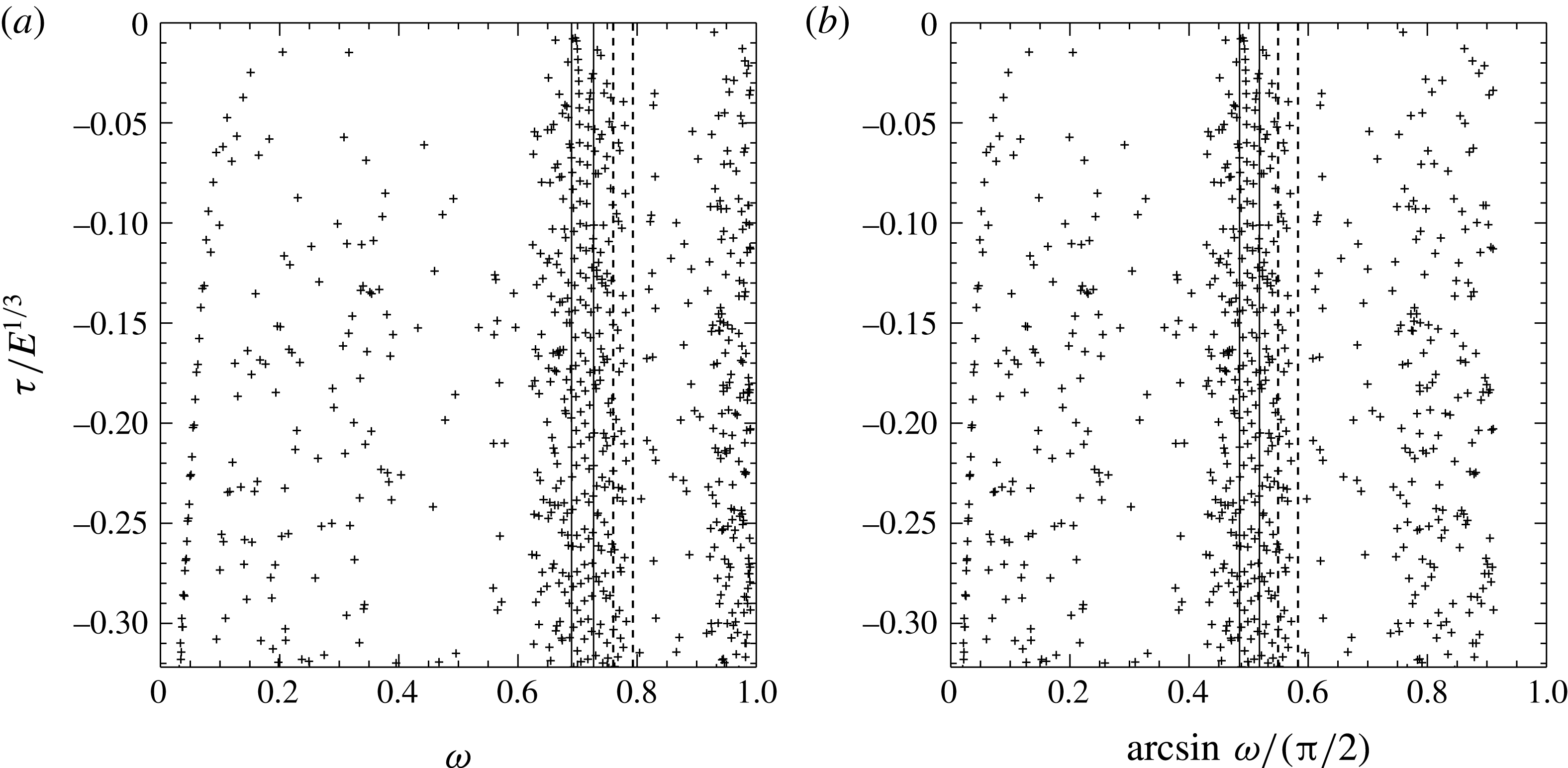
(a) Distribution of eigenvalues of inertial modes in the complex plane. (b) Same as (a) but the frequency has been converted into an angle (the critical latitude) scaled by
 $\unicode[STIX]{x03C0}/2$
. The dashed vertical lines delineate the part of the complex plane that is magnified in figure 3 while the solid vertical lines outline the part of the complex plane shown in figure 8(a). The Ekman number is set to
 $10^{-8}$
,
 $\unicode[STIX]{x1D702}=0.35$
and the numerical resolution is
 $L_{max}=800$
and
 $N_{r}=300$
. In both panels the real part has been rescaled by
 $E^{1/3}$
.

3 Numerical results
The numerical investigation of the foregoing eigenvalue problem that we shall now further present has revealed several types of eigenmodes.
We shall restrict ourselves in the following to modes that are symmetric with respect to the equator. The classification is based on the path of characteristics associated with the Poincaré equation. We recall that system (2.1) can be reduced to a single equation for the pressure perturbation, namely (1.1) when viscosity is set to zero. In the dimensionless expression of the equation, the frequency of the oscillation
 $\unicode[STIX]{x1D714}$
is necessarily less than unity. Associated characteristic surfaces are cones (or parts of cones) characterized by their opening angle
 $\unicode[STIX]{x1D703}^{c}=\arcsin \unicode[STIX]{x1D714}$
and an apex on the rotation axis.
 $\unicode[STIX]{x1D703}^{c}$
is also the critical latitude. This is the latitude where the characteristic surfaces are tangent to the spheres. Even for non-axisymmetric modes, characteristic surfaces are axisymmetric cones (Rieutord et al.
Reference Rieutord, Georgeot and Valdettaro2001). This is why we shall always visualize the characteristic cones by their trace in a meridian plane where they appear as straight lines. As Rieutord et al. (Reference Rieutord, Georgeot and Valdettaro2001) have shown, the path of the characteristic lines in a meridian plane generally converges towards a closed periodic orbit that is called an attractor. Exceptions are a finite number of frequencies that read
 $\sin (p\unicode[STIX]{x03C0}/q)$
where
 $p$
and
 $q$
are integers. For these frequencies any trajectory is periodic and there is no attractor. The number of such frequencies depends on the aspect ratio of the shell. For
 $\unicode[STIX]{x1D702}=0.35$
, periodic orbits with
 $p=1$
exist only for
 $q=3,4,6,8$
(Rieutord et al.
Reference Rieutord, Georgeot and Valdettaro2001).
To set the stage, we show in figure 1 a general view of the distribution of eigenvalues associated with viscous inertial modes in the complex plane. These eigenvalues have been computed through a systematic scan of the least-damped part of the complex plane with the Arnoldi–Chebyshev algorithm. It extends figure 17 of Rieutord et al. (Reference Rieutord, Georgeot and Valdettaro2001). When the imaginary part of the eigenvalues (the frequency) is converted into an angle (actually the critical latitude), the approximate symmetry with respect to latitude
 $\unicode[STIX]{x03C0}/4$
is emphasized. This symmetry is verified by characteristics trajectories, but not by the eigenfunctions since the rotation axis is of course not the same as the equator. The distribution of eigenvalues reflects this symmetry near
 $\unicode[STIX]{x03C0}/4$
, but this symmetry weakens when the critical latitude of the modes moves away from
 $\unicode[STIX]{x03C0}/4$
.
This general view of the complex plane clearly shows that the distribution is not uniform and no simple quantization, or quantum numbers, controls it. However, some regularities appear: a crowded region near
 $\unicode[STIX]{x03C0}/4$
(quasi-regular modes), deserted regions around
 $\unicode[STIX]{x03C0}/6$
and
 $\unicode[STIX]{x03C0}/3$
and some deep frequency bands where modes are strongly damped.
As shown by Rieutord et al. (Reference Rieutord, Georgeot and Valdettaro2001), this distribution of eigenvalues is profoundly marked by the orbits of characteristics and the attractors they may form. We have found three categories of modes, which we termed as attractor modes, critical latitude modes and quasi-regular modes.
3.1 Attractor modes
Attractor modes are modes associated with a specific attractor represented by a periodic orbit of characteristics. These modes were first studied in Rieutord & Valdettaro (Reference Rieutord and Valdettaro1997), and their analytic expression has been given by Rieutord et al. (Reference Rieutord, Valdettaro and Georgeot2002) in the two-dimensional case. We recall that the two-dimensional case refers to the same case as the one described by equation (2.1) but where curvature terms (like
 $(1/r)(\unicode[STIX]{x2202}/\unicode[STIX]{x2202}r)$
) of the spherical geometry are dismissed. This case is also referred to as the case of the slender torus, which is a torus with a large aspect ratio. Rieutord et al. (Reference Rieutord, Valdettaro and Georgeot2002) have shown that it can describe inertial modes that are trapped in the equatorial region of a thin spherical shell.
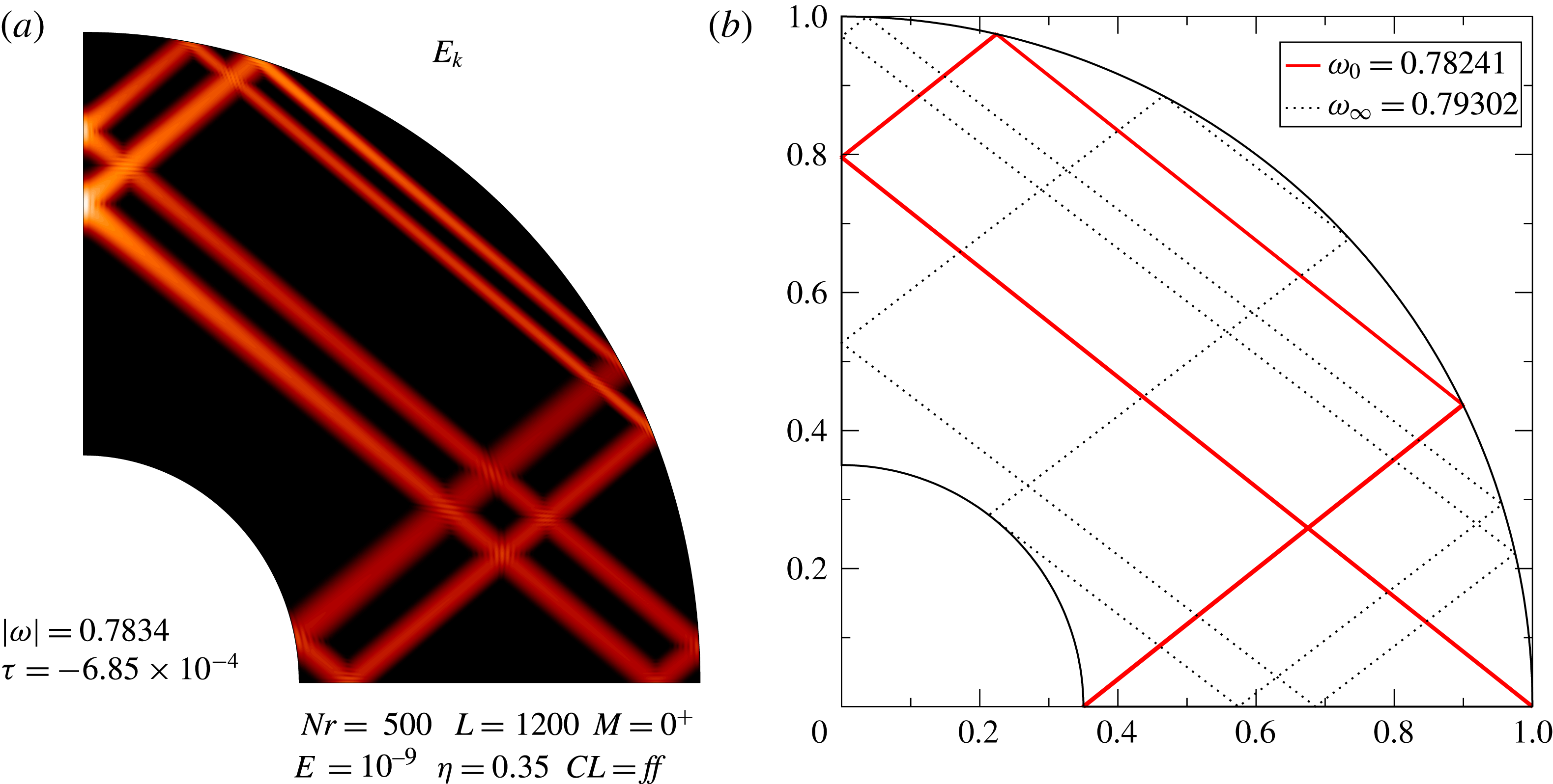
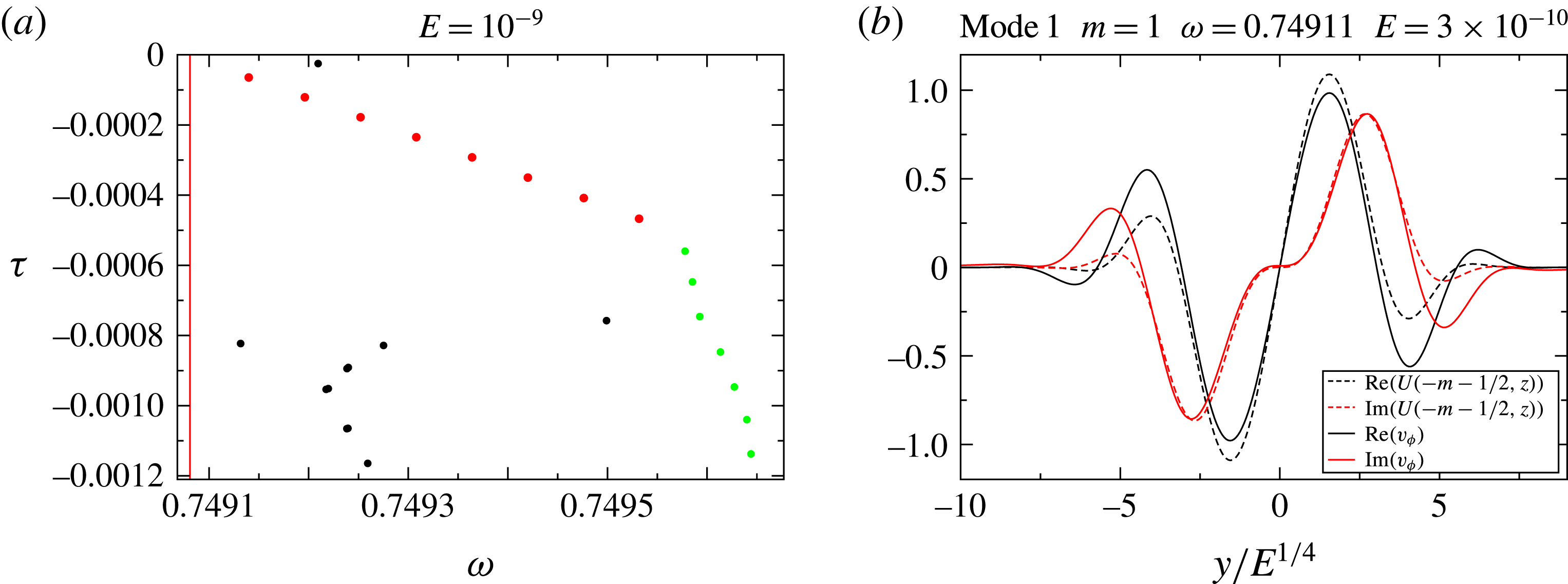
(a) The least-damped eigenmode associated with the attractor at
 $\unicode[STIX]{x1D714}=0.7834$
and
 $E=10^{-9}$
. The numerical resolution is
 $L_{\text{max}}=1200$
,
 $N_{r}=500$
. (b) Red line: the asymptotic attractor
 $\unicode[STIX]{x1D714}_{0}\simeq 0.782413$
associated with the mode in (a). Black-dotted line: the same attractor at the upper frequency limit
 $\unicode[STIX]{x1D714}=\unicode[STIX]{x1D714}_{\infty }\simeq 0.793$
.

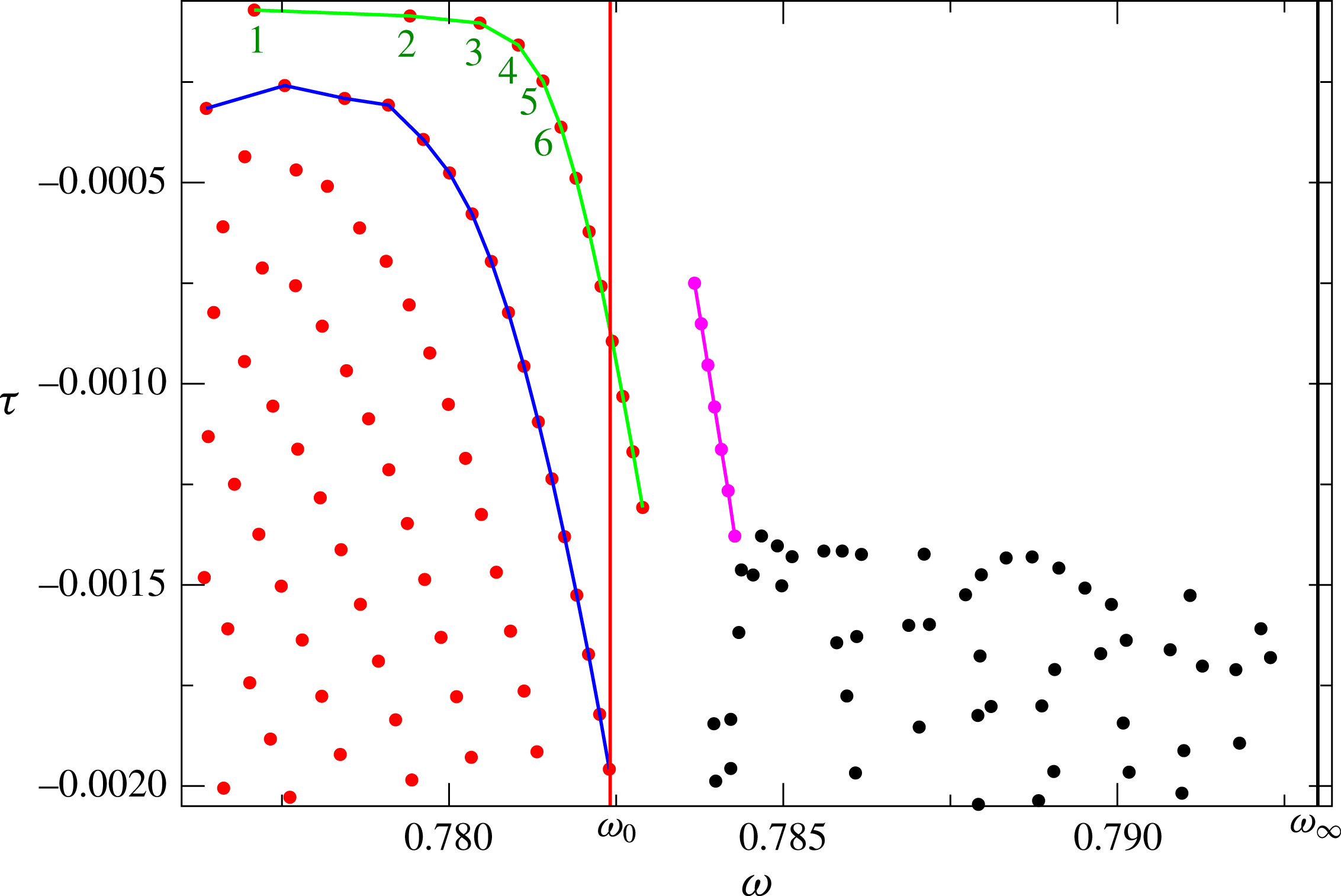
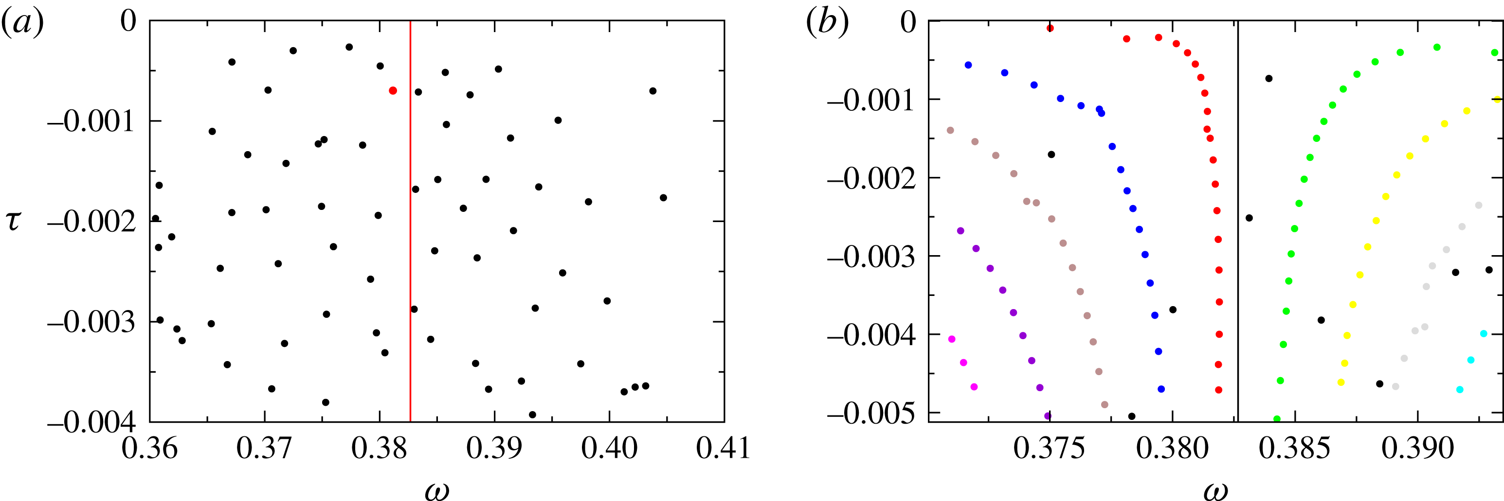
Distribution of eigenvalues in the complex plane around the frequency 0.785 for
 $\unicode[STIX]{x1D702}=0.35$
and
 $E=3\times 10^{-9}$
. The corresponding attractor is shown in figure 2.
 $\unicode[STIX]{x1D714}_{0}$
and
 $\unicode[STIX]{x1D714}_{\infty }$
are the frequency bounds of the attractor. Red dots show eigenvalues associated with critical latitude modes while black dots show eigenvalues associated with attractor modes. The purple eigenvalues have been computed with extended precision.

In figure 2(a) we show one such attractor mode. Eigenmodes featured in this attractor have eigenfrequencies in the interval
 $[\unicode[STIX]{x1D714}_{0},\unicode[STIX]{x1D714}_{\infty }]$
where
 $\unicode[STIX]{x1D714}_{0}\simeq 0.782413$
and
 $\unicode[STIX]{x1D714}_{\infty }\simeq 0.793$
for
 $\unicode[STIX]{x1D702}=0.35$
. In figure 2(b), we show the limiting shapes of this attractor when
 $\unicode[STIX]{x1D714}=\unicode[STIX]{x1D714}_{0}$
or
 $\unicode[STIX]{x1D714}=\unicode[STIX]{x1D714}_{\infty }$
. We recall that the strength of an attractor may be characterized by a (negative) Lyapunov exponent that measures the rate at which characteristics converge towards the attractor.
 $\unicode[STIX]{x1D714}_{0}$
and
 $\unicode[STIX]{x1D714}_{\infty }$
refer to the values where the Lyapunov exponent is respectively zero or
 $-\infty$
. In the former case, characteristics are still converging towards the attractor but algebraically, while in the latter case they touch the critical latitude making the mapping (featured by the characteristics) infinitely contracting (see Rieutord et al.
Reference Rieutord, Georgeot and Valdettaro2001, for a more detailed discussion). Note that the asymptotic frequency
 $\unicode[STIX]{x1D714}_{0}$
of the figure 2 attractor is easily expressed as a function of the aspect ratio
 $\unicode[STIX]{x1D702}$
and reads
 $$\begin{eqnarray}\unicode[STIX]{x1D714}_{0}=\sqrt{{\displaystyle \frac{3+\sqrt{5-4\unicode[STIX]{x1D702}}}{8}}}.\end{eqnarray}$$
In figure 3, we now show the part of the complex plane where the eigenvalues of this attractor show up. The vertical lines delineate the limiting frequencies
 $\unicode[STIX]{x1D714}_{0}$
and
 $\unicode[STIX]{x1D714}_{\infty }$
. We immediately note that eigenvalues are distributed in several subsets. In the interval
 $[\unicode[STIX]{x1D714}_{0},\unicode[STIX]{x1D714}_{\infty }]$
, the purple dots show the eigenvalues associated with the attractor modes, while the black dots are affected by numerical noise (see below). At frequencies lower than
 $\unicode[STIX]{x1D714}_{0}$
, we note a neat organization of the eigenvalues (red dots), which is associated with the set of ‘critical latitude modes’. We discuss these latter modes in the next section.
Remarkably, the eigenvalues of the attractor modes (the purple dots in figure 3) seem to be governed by the following law:
 $$\begin{eqnarray}\unicode[STIX]{x1D706}_{n}=\text{i}\unicode[STIX]{x1D714}_{0}-2\hat{\unicode[STIX]{x1D70F}}_{1}\text{e}^{\text{i}\unicode[STIX]{x1D719}_{1}}\mathit{E}^{1/3}-\left(n+{\textstyle \frac{1}{2}}\right)\text{e}^{\text{i}\unicode[STIX]{x1D719}_{2}}\sqrt{2}\hat{\unicode[STIX]{x1D70F}}_{2}\mathit{E}^{1/2}+\cdots \,.\end{eqnarray}$$
In this expression,
 $\unicode[STIX]{x1D714}_{0}$
is the asymptotic frequency of the attractor (as given by (3.1)), while
 $\hat{\unicode[STIX]{x1D70F}}_{1}$
and
 $\hat{\unicode[STIX]{x1D70F}}_{2}$
are positive real numbers of order unity that depend on the shape of the attractor.
 $n$
is the quantum number that characterizes the mode. We use the term ‘quantization’ in this context to signify that eigenvalues are arranged along specific lines in the complex plane and are distributed with some regularity along such lines. We note that the
 $n+1/2$
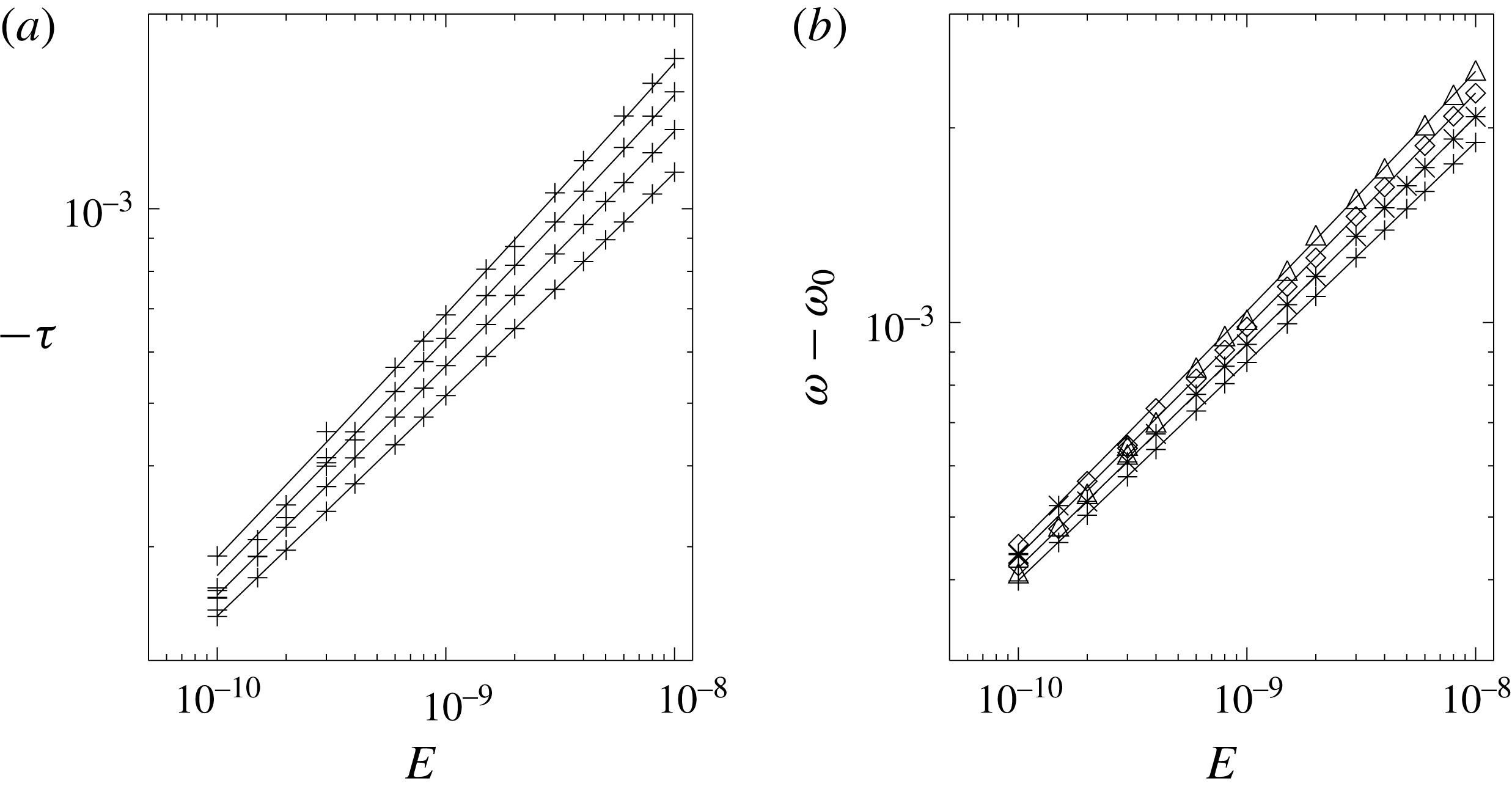
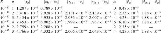
factor is reminiscent of the energy levels of a quantum particle in a parabolic well, and of the eigenvalues of the two-dimensional problem of Rieutord et al. (Reference Rieutord, Valdettaro and Georgeot2002). In figure 4, we illustrate the good matching of the real and imaginary parts of the eigenvalues with the law (3.2).
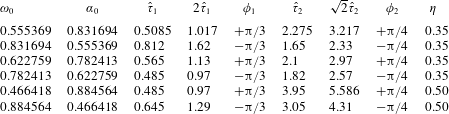
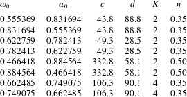
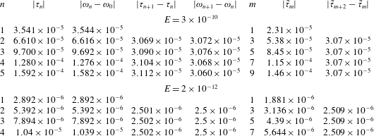
We have found such sets of eigenvalues in association with various attractors. Table 1 gives the parameters for six sets of such modes. In this table, we gathered the families of modes by pairs of families where we associated the attractor at
 $\unicode[STIX]{x1D714}_{0}$
with the symmetric one at
 $\unicode[STIX]{x1D6FC}_{0}=\sqrt{1-\unicode[STIX]{x1D714}_{0}^{2}}$
. The symmetry is with respect to latitude
 $\unicode[STIX]{x03C0}/4$
. We note that the phases
 $\unicode[STIX]{x1D719}_{1}$
or
 $\unicode[STIX]{x1D719}_{2}$
in (3.2) are opposite for pairs of attractors. This betrays the fact that
 $\unicode[STIX]{x1D714}_{\infty }<\unicode[STIX]{x1D714}<\unicode[STIX]{x1D714}_{0}$
when the frequency is less than
 $1/\sqrt{2}$
while
 $\unicode[STIX]{x1D714}_{\infty }>\unicode[STIX]{x1D714}>\unicode[STIX]{x1D714}_{0}$
when
 $\unicode[STIX]{x1D714}>1/\sqrt{2}$
. Now, we observe that the symmetry of attractors, with respect to latitude
 $\unicode[STIX]{x03C0}/4$
, is not verified by the modes since the
 $\hat{\unicode[STIX]{x1D70F}}_{1}$
and
 $\hat{\unicode[STIX]{x1D70F}}_{2}$
coefficients are not the same for a family and its symmetric. The
 $\hat{\unicode[STIX]{x1D70F}}_{1}$
and
 $\hat{\unicode[STIX]{x1D70F}}_{2}$
coefficients are therefore sensitive to the reflection on the rotation axis. We remark that there are attractors with
 $\unicode[STIX]{x1D714}_{0}<\unicode[STIX]{x1D714}<\unicode[STIX]{x1D714}_{\infty }$
for frequencies less than
 $1/\sqrt{2}$
(like the ones with
 $\unicode[STIX]{x1D714}_{0}=0.35866$
and
 $\unicode[STIX]{x1D714}_{\infty }=0.36134$
) and correspondingly
 $\unicode[STIX]{x1D714}_{0}>\unicode[STIX]{x1D714}>\unicode[STIX]{x1D714}_{\infty }$
when
 $\unicode[STIX]{x1D714}>1/\sqrt{2}$
. However, we did not find any set of eigenvalues associated with those attractors. To be complete, we note that there exist attractor modes whose eigenvalues cannot be represented by (3.2). Since no clear law seems to govern their properties, we shall not discuss them any further in the present work.
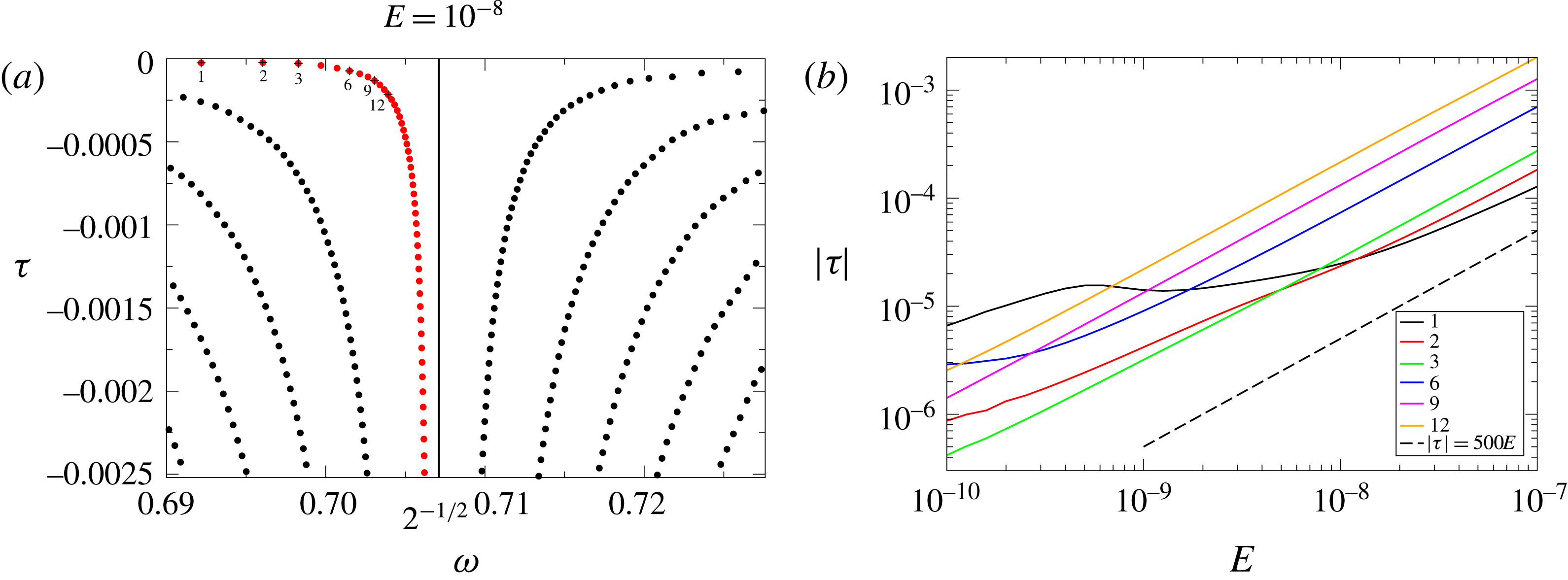
(a) Damping rate for the four least-damped eigenvalues of the 0.782-attractor modes as a function of the Ekman number. Pluses indicate the numerical values and the solid lines show the law (3.2). (b) Same as (a) but for the deviation of the frequency from the frequency of the asymptotic attractor.

Asymptotic parameters of six modes following (3.2).

Eigenvalue spectrum of attractor modes in the complex plane.
 $\unicode[STIX]{x1D70F}$
is the real part and
 $\unicode[STIX]{x1D714}$
is the imaginary part. (a) A double precision calculation, (b) with extended precision. In both panels the resolution is
 $L_{max}=440$
and
 $N_{r}=160$
. The attractor exists at frequencies below
 $\unicode[STIX]{x1D714}_{0}=0.583$
which is visualized by a red line. The aspect ratio is
 $\unicode[STIX]{x1D702}=0.50$
. This attractor is the one corresponding to 0.555 when
 $\unicode[STIX]{x1D702}=0.35$
(e.g. Rieutord et al.
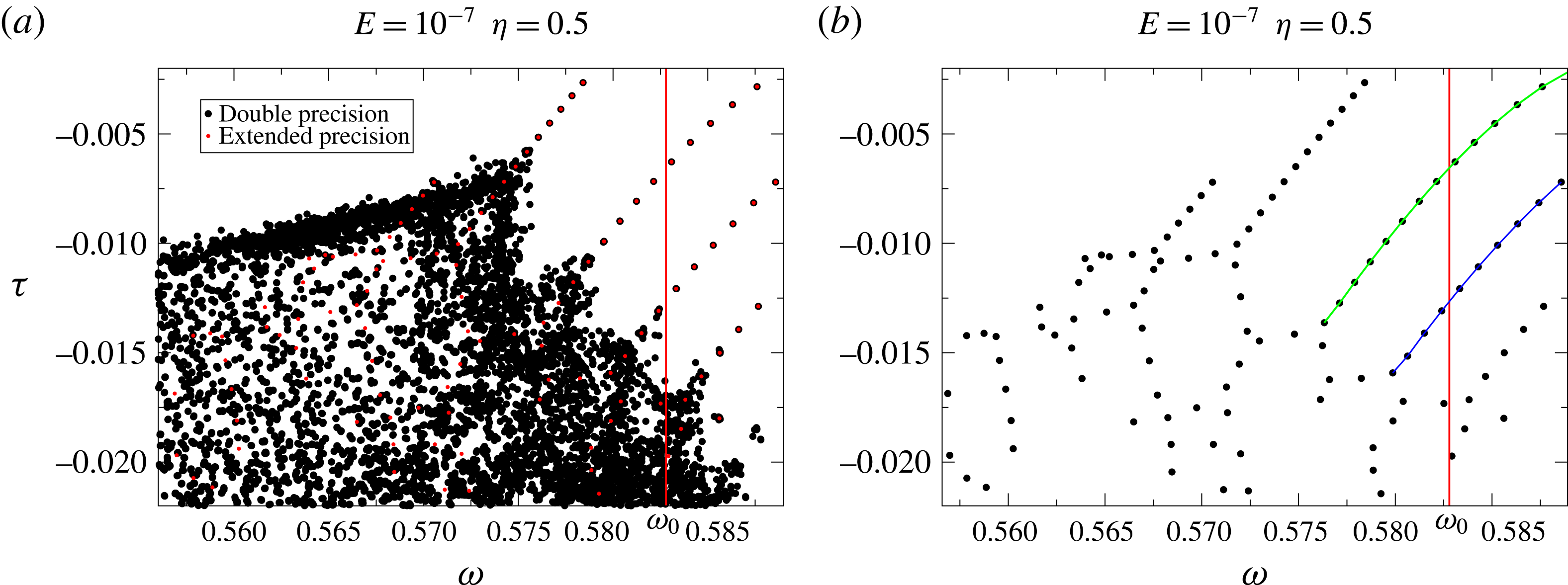
Reference Rieutord, Georgeot and Valdettaro2000). The green and blue lines emphasize two families of critical latitude modes (see § 3.2).

Round-off errors are actually a major plague of eigenvalue/eigenmode computation of attractor modes. We see in figure 3 that the black dots associated with attractor modes are randomly distributed unlike the least-damped modes (purple dots) which obey the dispersion relation (3.2). In fact, eigenvalues of the more-damped modes are strongly perturbed by round-off errors.
(a) and (c) The viscous dissipation for the first and second eigenmodes of the ‘green family’ shown in figure 3. The Ekman number is
 $3\times 10^{-9}$
, for which we used
 $L_{max}=1200$
,
 $N_{r}=500$
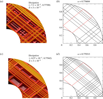
. Most intense values are in yellow. We also added an artificial depth (yellow curves are on top) to better distinguish the shapes. Panels (b) and (d) show the corresponding web of characteristics. The red rectangle shows the periodic orbit drawn by the characteristic emitted towards the North from the critical latitude.

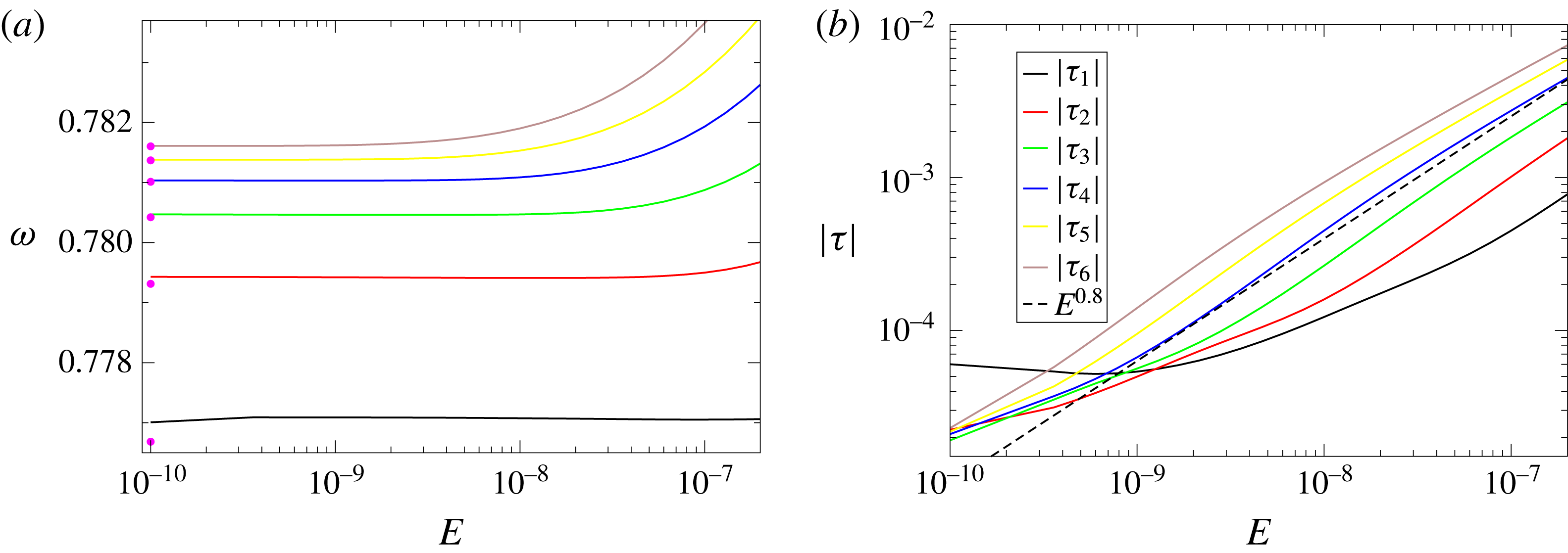
(a) Dependence of the frequency of the ‘green family’ modes of figure 3 on the Ekman number. The pink dots mark the frequencies of the webs of rays that connect the North and South critical latitudes of the internal sphere. (b) Same as in (a) but for the damping rates. The numbers refer to the numbering of the mode in figure 3.

In figure 5, we further illustrate this phenomenon. Figure 5(a) (respectively figure 5
b) shows the double (respectively extended) precision calculation of the distribution of eigenvalues associated with attractor modes (for this attractor
 $\unicode[STIX]{x1D714}_{\infty }<\unicode[STIX]{x1D714}_{0}$
). The plotted eigenvalues are actually superpositions of several independent calculations. In each calculation we have only changed the shift parameter of equation (2.10). As was shown in Valdettaro et al. (Reference Valdettaro, Rieutord, Braconnier and Fraysse2007), a noisy distribution of eigenvalues is related to the sensitivity of matrices
 $[\unicode[STIX]{x1D63C}]$
and
 $[\unicode[STIX]{x1D63D}]$
to small perturbations, so ultimately to round-off errors. In (a), we see that families governed by a dispersion relation disappear in a bath of randomly distributed eigenvalues at large damping rates. When the same distribution is computed with extended precision (quadruple precision, b), the noisy distribution leaves the place to an ordered distribution of eigenvalues. In this same figure we also note that some branches cross the line marking the asymptotic frequency
 $\unicode[STIX]{x1D714}_{0}$
of the attractor. Examination of the modes along this branch reveals that they are still featured by the asymptotic attractor, despite the fact that the propagation of characteristics does not show the attractor. The eigenfunctions whose eigenfrequency is neatly above
 $\unicode[STIX]{x1D714}_{0}$
actually show that the modes of such a branch are featured by the shear layer emitted towards North by the critical latitude singularity. The associated characteristics trajectory shows that the shear layer has to wind around the former attractor before leaving it. However, because of viscosity, the winding stops at some stage still leaving the trace of the attractor. Hence the branches can continuously cross the
 $\unicode[STIX]{x1D714}_{0}$
line. We surmise that for asymptotically small values of the Ekman number such crossing is not possible because trajectories of characteristics may bifurcate towards another attractor. In the next subsection we shall investigate such branches of modes.
3.2 Modes associated with the critical latitude of the inner sphere
Beside the modes that are associated with a periodic attractor, the spectra (figures 3 and 5) display other obvious families of modes. In figure 6(a,c), we show the two modes numbered 1 and 2 of the green family of figure 3, with their associated path of characteristics (figure 6 b,d). With these meridional cuts, we clearly see that the characteristic emitted by the northern critical latitude of the inner shell in the southern direction finally reaches the equator of the outer shell. This means, by symmetry, that it joins the southern critical latitude on the inner shell. The shear layer issued from the northern critical latitude towards the North loops back to the same critical latitude as shown by the red path in figure 6.
From the plots of figure 6, we note that the quantization of these modes seems to come from the length of the path connecting the North and South critical latitudes on the inner sphere. The path is not unique and a slight change in the frequency increases the number of rays in the bulk by two units. In figure 7(a), we show that the discrete frequencies of the green family can almost be retrieved by the simple geometrical rule of finding a path of characteristics that connects the North and South critical latitudes. The same is true for the blue family, which is characterized by more dissipative shear layers (the transverse wavenumber is higher). The evolution of the damping rate of these modes with the Ekman number is not standard, as may be seen in figure 7(b). Indeed, for the first mode (tagged 1 in figure 3), below
 $E=10^{-9}$
, the damping rate increases while the Ekman number decreases. We explain this behaviour as a consequence of the activation of the northern branch of the shear layer that loops back to the critical latitude (red segments in figure 6), which is a place of high dissipation. If the Ekman number is low enough, this loop has a larger amplitude and has a larger contribution to the damping rate of the mode. Most likely, ‘critical latitude modes’ are not asymptotic and may only exist in a finite range of Ekman numbers.
(a) Spectrum near the frequency
 $\sin (\unicode[STIX]{x03C0}/4)$
. (b) Damping rate as a function of
 $E$
for the modes numbered
 $1,2,3,6,9,12$
in (a). The dashed line is
 $|\unicode[STIX]{x1D70F}|=500E$
.




3.3 The quasi-regular modes
In the distribution of eigenvalues shown in figure 1, we noticed a set of eigenvalues with very low damping rates gathered around the frequency
 $\sin (\unicode[STIX]{x03C0}/4)$
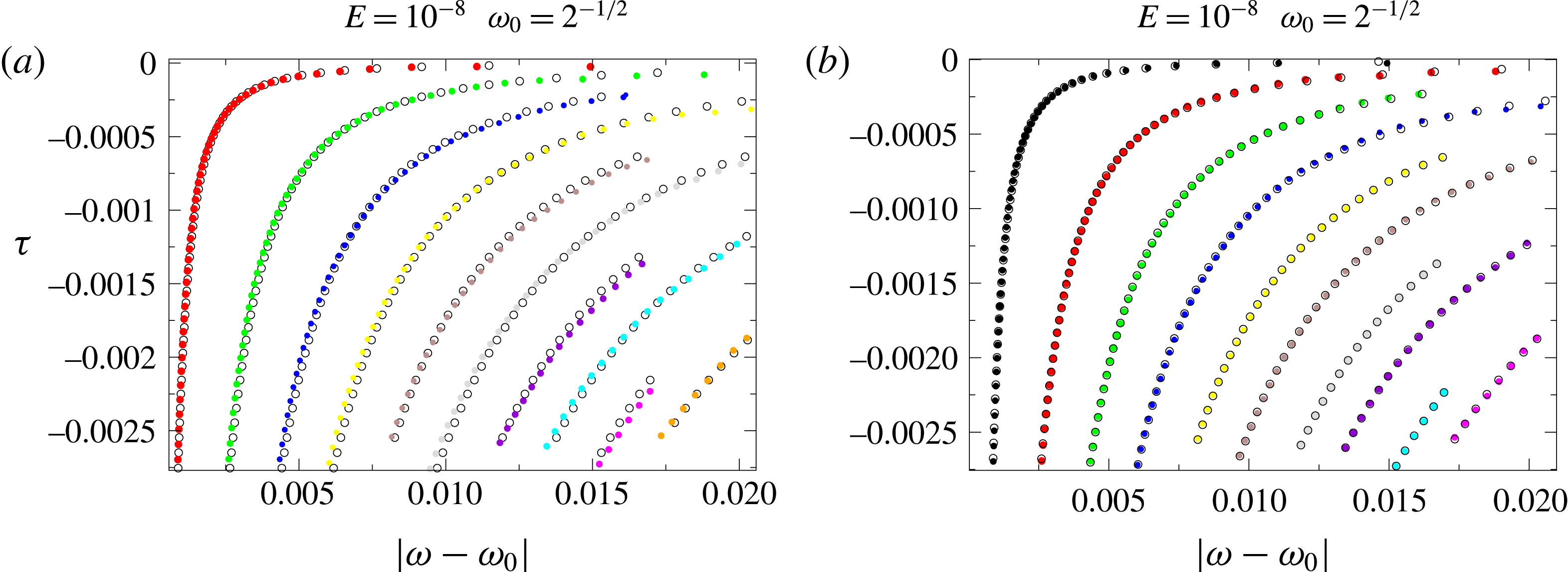
. A close-up view of this region of the complex plane, displayed in figure 8(a), shows that this set of eigenvalues has peculiar properties that deserve some attention. First, we note that the eigenvalues seem to obey simple quantization rules as their distribution clearly follows specific lines in the complex plane. In addition, their damping rate is almost proportional to the Ekman number in some range of this parameter (e.g. figure 8
b). These features give evidence of a quasi-regular nature of this kind of mode. We recall that regular eigenmodes have a structure that is weakly dependent on viscosity and which converges to a smooth eigenfunction in the inviscid limit. We thus call these modes quasi-regular since they are similar to truly regular modes in some Ekman number range, but they lose this character below some Ekman number specific to the mode (see below).
The specific distribution of eigenvalues in this region of the complex plane can be explained with some simple arguments based on the properties of the web of characteristics.
First, we may observe that the non-symmetric distribution of eigenvalues with respect to the line
 $\unicode[STIX]{x1D714}=\sin (\unicode[STIX]{x03C0}/4)$
actually reflects an alternate distribution of the branches on each side of the
 $\unicode[STIX]{x1D714}=\sin (\unicode[STIX]{x03C0}/4)$
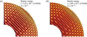
line, as shown by figure 9. Second, we observe that the actual eigenmodes are featured by the web of characteristics. The modes show periodic structures (e.g. figures 10 and 11) even if characteristics do not follow periodic orbits (this is possible only when
 $\unicode[STIX]{x1D714}=\sin (\unicode[STIX]{x03C0}/4)$
).
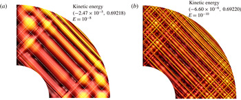
(a) Meridional distribution of the kinetic energy of the eigenmode associated with eigenvalue tagged ‘1’ in figure 8 at
 $E=10^{-8}$
. (b) Same as in (a) but for
 $E=10^{-10}$
. In (a) we have superposed the path of the characteristic started northward at the equator taking the same frequency as the mode.


The propagation of characteristics associated with a mode frequency is nevertheless interesting. Characteristics are indeed showing the path of energy but also the location of equiphase lines (recall that the group and phase velocities are orthogonal for inertial waves). Hence, the distance between two parallel characteristics (e.g. figures 10
a or 11
a) may be interpreted as the typical wavelength of the mode. Let us consider a mode whose frequency is slightly different from
 $\sin (\unicode[STIX]{x03C0}/4)$
. Let us say that
 $$\begin{eqnarray}\unicode[STIX]{x1D714}=\sin \left({\displaystyle \frac{\unicode[STIX]{x03C0}}{4}}\pm \unicode[STIX]{x1D700}\right),\quad \text{with }\unicode[STIX]{x1D700}\ll 1.\end{eqnarray}$$
The distance between the two characteristics of negative slope with one issued from the equator of the outer sphere is
 $$\begin{eqnarray}\unicode[STIX]{x1D6EC}={\displaystyle \frac{\sin (2\unicode[STIX]{x1D700})}{\sin (\unicode[STIX]{x03C0}/4)}}\end{eqnarray}$$
but from (3.3) we have
 $$\begin{eqnarray}\unicode[STIX]{x1D714}-\sin (\unicode[STIX]{x03C0}/4)=\pm \unicode[STIX]{x1D700}\cos (\unicode[STIX]{x03C0}/4)\end{eqnarray}$$
at first order. Hence, the typical wavelength of the mode is
 $$\begin{eqnarray}\unicode[STIX]{x1D6EC}\simeq 4|\unicode[STIX]{x1D714}-\sin (\unicode[STIX]{x03C0}/4)|,\end{eqnarray}$$
where we assumed
 $\unicode[STIX]{x1D6EC}>0$
. Thus the damping rate of the mode should scale like
 $$\begin{eqnarray}\unicode[STIX]{x1D70F}\sim -4\unicode[STIX]{x03C0}^{2}E/\unicode[STIX]{x1D6EC}^{2}={\displaystyle \frac{E\unicode[STIX]{x03C0}^{2}}{4(\unicode[STIX]{x1D714}-\sin (\unicode[STIX]{x03C0}/4))^{2}}}.\end{eqnarray}$$
Thus for a given set of modes (a branch) we expect that
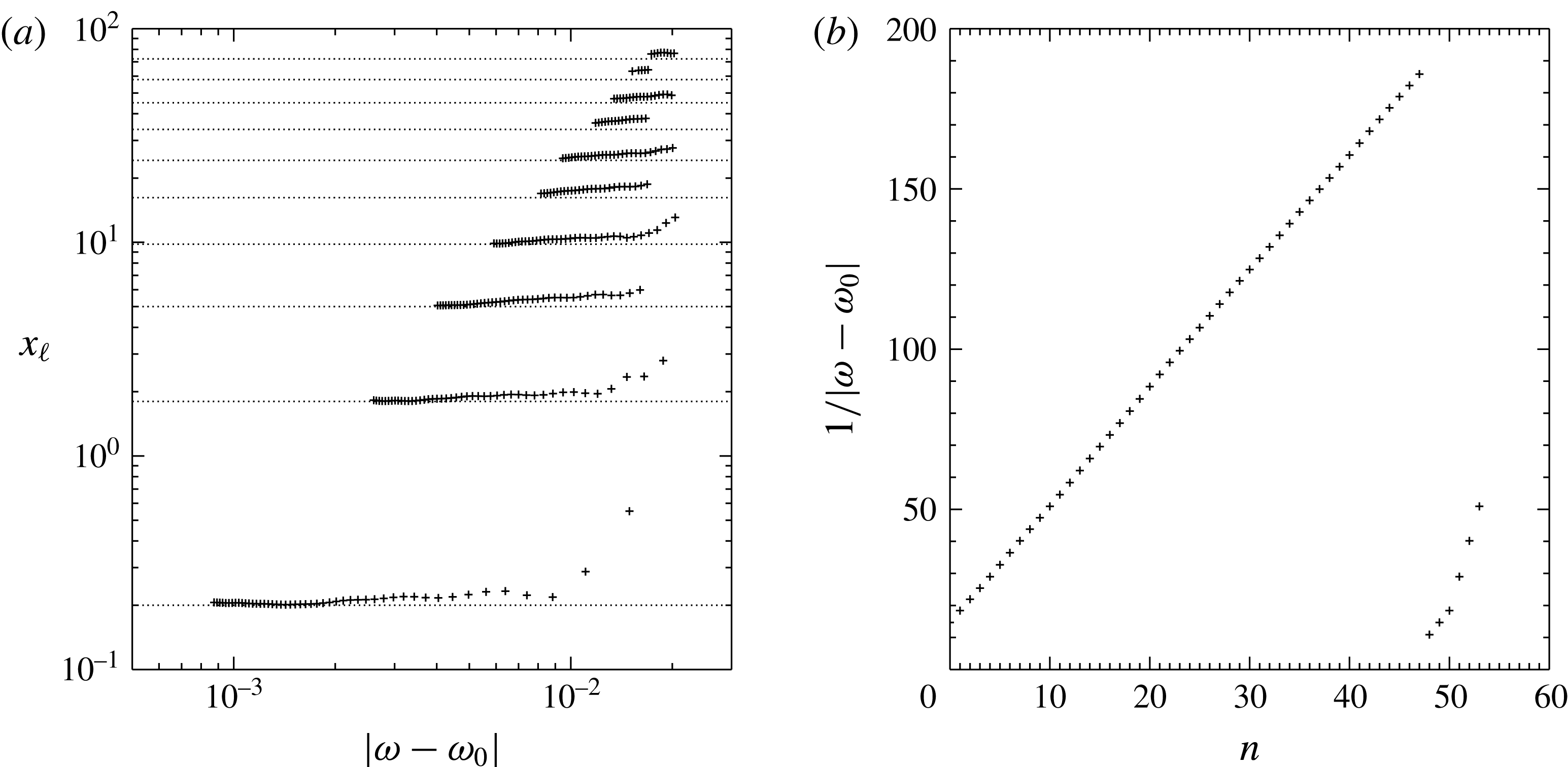
 $$\begin{eqnarray}\unicode[STIX]{x1D70F}(\unicode[STIX]{x1D714}-\sin (\unicode[STIX]{x03C0}/4))^{2}=-Ex_{\ell },\end{eqnarray}$$
where
 $x_{\ell }$
is a constant specific to the branch. As shown in figure 12(a),
 $x_{\ell }$
is indeed a constant. Actually, the constant
 $x_{\ell }$
is quantized in a simple way:
 $$\begin{eqnarray}x_{\ell }\simeq {\textstyle \frac{4}{5}}(\ell +1/2)^{2},\quad \text{with }\ell =0,1,\ldots .\end{eqnarray}$$
This expression is derived from a numerical fit. It betrays again the quantization of the harmonic oscillator, showing that each branch corresponds to a different state of this oscillator. Unfortunately, we could not recover this formula from a simple theoretical argument.
(a) Quantization of the branches: for all the eigenvalues shown in figure 8 the quantity
 $(\unicode[STIX]{x1D714}-\sin (\unicode[STIX]{x03C0}/4))^{2}\unicode[STIX]{x1D70F}/E$
is plotted versus
 $|\unicode[STIX]{x1D714}-\sin (\unicode[STIX]{x03C0}/4)|$
(pluses). The dotted lines show the expected formula
 $x_{\ell }=(4/5)\left(\ell +1/2\right)^{2}$
. (b) Quantization along the first branch:
 $1/|\unicode[STIX]{x1D714}-\sin (\unicode[STIX]{x03C0}/4)|$
versus the order of the eigenvalue.

We may however proceed a little further if we look for the quantization along a given branch. Comparison of two modes of a branch (e.g. figures 10 and 11) shows that they differ by their typical wavelength along the radius. (For modes in the second branch (green dots in figure 9 a) with a similar frequency as the modes of the first branch (red dots), the same shape as in figure 10 is observed but the dominant wavenumber is increased by some factor.) Thus, we also should expect from (3.6) that
 $$\begin{eqnarray}|\unicode[STIX]{x1D714}-\sin (\unicode[STIX]{x03C0}/4)|\propto {\displaystyle \frac{1-\unicode[STIX]{x1D702}}{n}}.\end{eqnarray}$$
Figure 12(b) shows the linear behaviour of
 $1/|\unicode[STIX]{x1D714}-\sin (\unicode[STIX]{x03C0}/4)|$
with the rank of the eigenvalues of a branch. Hence, eigenvalues on a given branch seem to verify
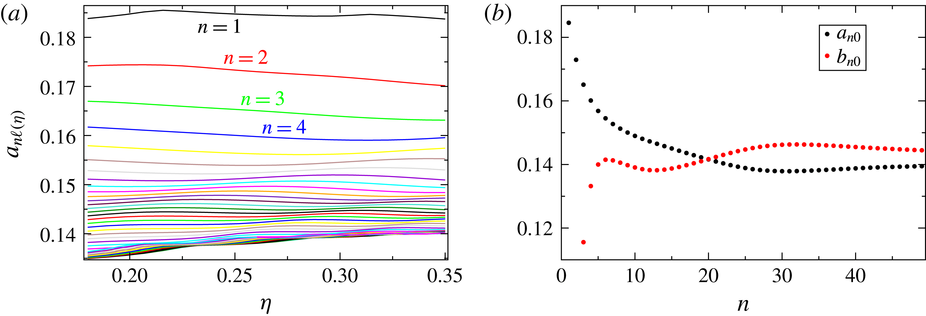
 $$\begin{eqnarray}|\unicode[STIX]{x1D714}_{n\ell }-\sin (\unicode[STIX]{x03C0}/4)|={\displaystyle \frac{a_{n\ell }(\unicode[STIX]{x1D702})(1-\unicode[STIX]{x1D702})(\ell +1/2)}{n}},\quad \unicode[STIX]{x1D70F}_{n\ell }=-{\displaystyle \frac{En^{2}}{\left[b_{n\ell }(\unicode[STIX]{x1D702})(1-\unicode[STIX]{x1D702})\right]^{2}}},\end{eqnarray}$$
with
 $a_{n\ell }(\unicode[STIX]{x1D702})$
and
 $b_{n\ell }(\unicode[STIX]{x1D702})$
real values that have a very mild dependence on
 $\unicode[STIX]{x1D702}$
. Their independence on
 $\unicode[STIX]{x1D702}$
is checked in figure 13(a): the curves are almost flat horizontal lines. From this figure we also see that the curves for larger
 $n$
(that are the lower ones) cluster very near the same value: this means that
 $a_{n\ell }$
and
 $b_{n\ell }$
do not vary much with
 $n$
(for large enough
 $n$
). We also checked that they do not depend much on
 $\ell$
. This is shown in figure 9(a) where we plot the eigenvalues given by the above formula using constant values for
 $a$
and
 $b$
, precisely those computed by best fit of formula (3.11) with the actual eigenvalues shown in figure 8. The best fit gives
 $a=0.141$
and
 $b=0.152$
, and we see from figure 9(a) that the actual and predicted eigenvalues match quite well, at least for
 $n$
large enough.
Actually an even better fitting formula for the spectrum in this region is found to be
 $$\begin{eqnarray}\unicode[STIX]{x1D70F}_{n\ell }=-E(9.89n-0.70\ell +0.26)^{2},\quad |\unicode[STIX]{x1D714}_{n\ell }-\sin (\unicode[STIX]{x03C0}/4)|={\displaystyle \frac{\ell +1/2}{11.35n-2.33\ell -15.02}}.\end{eqnarray}$$
It reproduces fairly well a large fraction of the eigenvalues as shown in figure 9(b).
In figure 13(b) we show the best fit of
 $a_{n0}$
(black points) and
 $b_{n0}$
(red points) obtained using the computed eigenvalues for
 $\unicode[STIX]{x1D702}$
in the range
 $0.18\leqslant \unicode[STIX]{x1D702}\leqslant 0.35$
. For a given value of
 $n$
the fit is done by computing the values
 $a_{n0}$
and
 $b_{n0}$
that minimize the error on
 $a_{n0}-a_{n0}(\unicode[STIX]{x1D702})$
and
 $b_{n0}-b_{n0}(\unicode[STIX]{x1D702})$
. We confirm that, apart from the first values of
 $n$
for which we have remarked previously that the smooth behaviour at
 $E=10^{-8}$
is already lost (see figure 8
b), these values depend very little on
 $n$
, and moreover that they tend to very similar values for large
 $n$
: for example
 $a_{49,0}=0.139$
and
 $b_{49,0}=0.145$
.
(a) Variation with
 $\unicode[STIX]{x1D702}$
of the eigenvalues belonging to the red branch of figure 8. The curves plotted are
 $a_{n\ell }(\unicode[STIX]{x1D702})=n[\unicode[STIX]{x1D714}_{n\ell }-\sin (\unicode[STIX]{x03C0}/4)]/(1-\unicode[STIX]{x1D702})(\ell +1/2)$
for
 $n<50$
and
 $\ell =0$
. The top curves correspond to the lowest values of
 $n$
, thus to the least-damped eigenvalues. (b) Black: for each
 $n$
we plot the best fit of coefficient
 $a_{n0}(\unicode[STIX]{x1D702})$
of (3.11) as obtained from the data plotted in (a). Similarly we plot in red the best fit of coefficient
 $b_{n0}(\unicode[STIX]{x1D702})$
appearing in (3.11).

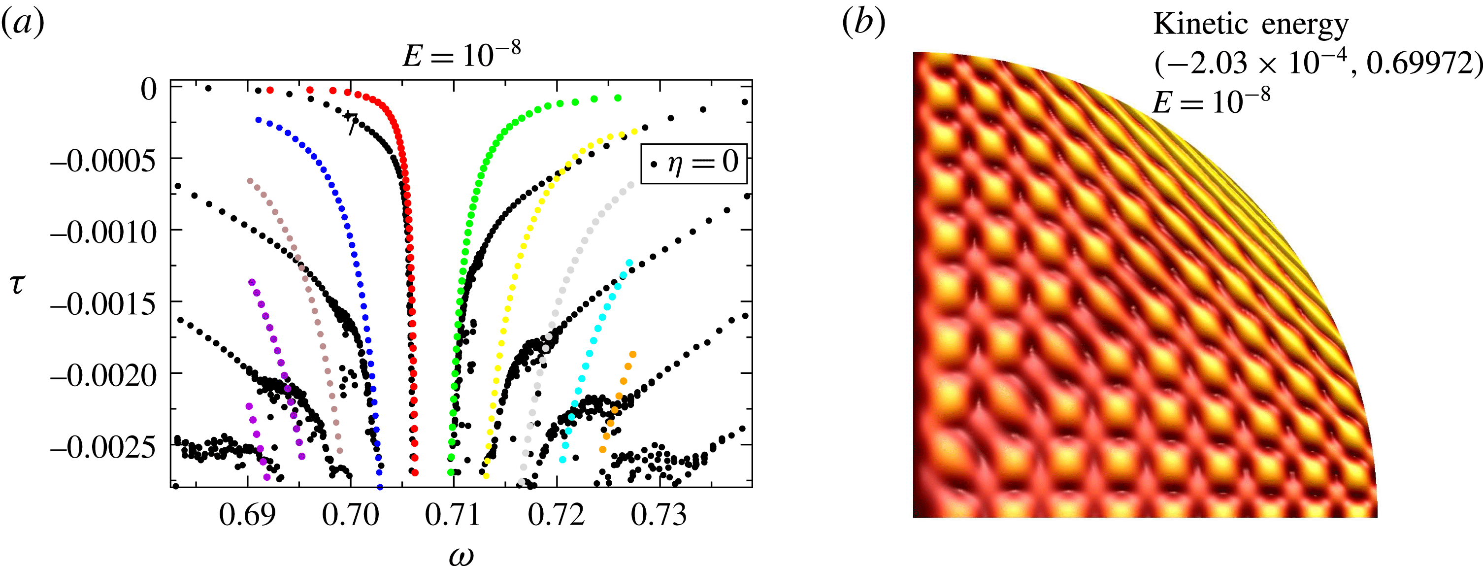
(a) Spectrum near the frequency
 $\sin (\unicode[STIX]{x03C0}/4)$
at Ekman number
 $E=10^{-8}$
. Black dots correspond to the full sphere
 $\unicode[STIX]{x1D702}=0$
. Coloured dots are for the spherical shell with aspect ratio
 $\unicode[STIX]{x1D702}=0.35$
. They are the same as in figure 8. (b) Kinetic energy for mode 7 of first branch at
 $\unicode[STIX]{x1D702}=0$
, the eigenvalue marked with a plus sign in panel (a). Note the similarity with the shape of eigenvalue 6 of the red family, shown in figure 11(a).

The foregoing results suggest that the eigenvalue spectrum has some universal features around
 $\sin (\unicode[STIX]{x03C0}/4)$
independent of the aspect ratio of the shell. Thus, we examined the eigenvalue spectrum of the full sphere (
 $\unicode[STIX]{x1D702}=0$
), for which eigenmodes exist even at zero Ekman number. The result is shown in figure 14(a) where we superpose the spectra of the spherical shell at
 $\unicode[STIX]{x1D702}=0.35$
and of the full sphere (
 $\unicode[STIX]{x1D702}=0$
). The noise in the very-damped modes of the full sphere is due to round-off errors. Nevertheless, we clearly recognize that the eigenvalues of the full sphere are also distributed in branches like those of the spherical shell. Corresponding branches of the full sphere and the spherical shell tend to merge in the strongly damped part of the spectrum. Figure 14(b) shows that the shape of a strongly damped regular mode of the full sphere is very similar to that of a quasi-regular mode of the shell (e.g. figure 11).
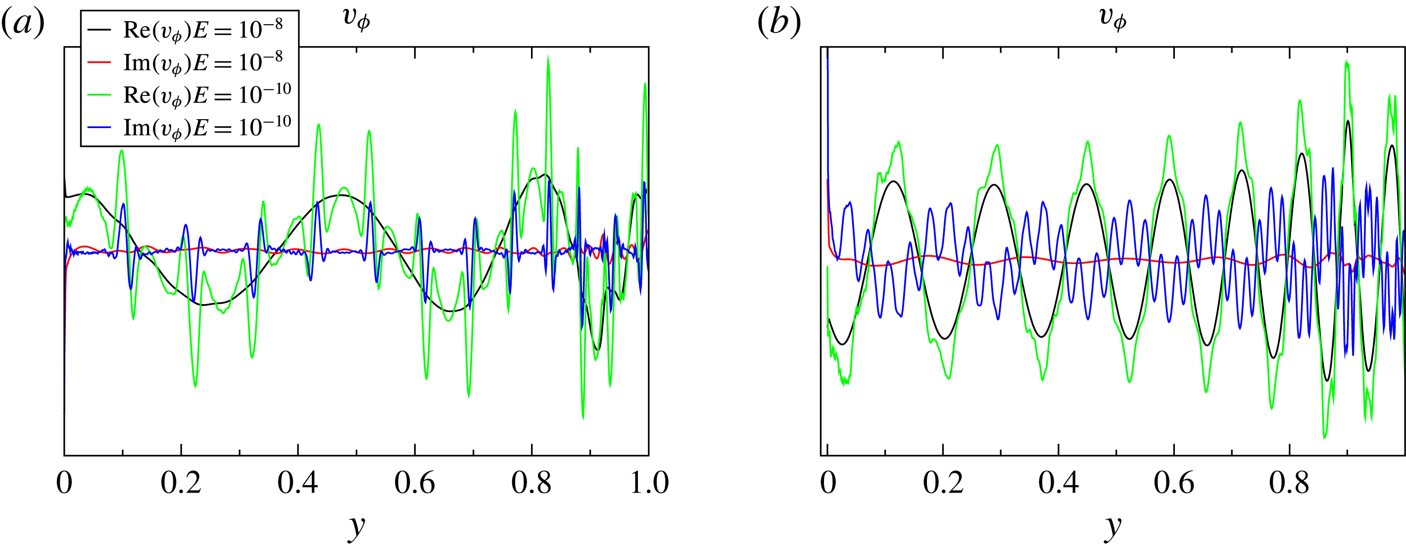
Profile of
 $v_{\unicode[STIX]{x1D719}}$
for mode tagged ‘1’ in figure 8(a) and mode 6 (b). The profile is shown along the radial direction starting from inner critical latitude. Note the smoothness of the black lines (
 $E=10^{-8}$
) and the emergence of small scales in the green lines (
 $E=10^{-10}$
).

Eigenvalue spectrum in the complex plane around
 $\unicode[STIX]{x1D714}=\sin (\unicode[STIX]{x03C0}/8)$
when
 $\unicode[STIX]{x1D702}=0.35$
(a), and when
 $\unicode[STIX]{x1D702}=0.2$
(b).

The foregoing results explain the ‘anti-resonance’ observed by Rieutord & Valdettaro (Reference Rieutord and Valdettaro2010) for tidally forced inertial modes when the forcing frequency equals
 $\sin (\unicode[STIX]{x03C0}/4)$
. As the forcing frequency tends to
 $\sin (\unicode[STIX]{x03C0}/4)$
the wavenumber of the excited modes tends to infinity, freezing any response of the fluid to a periodic forcing at
 $\unicode[STIX]{x1D714}=\sin (\unicode[STIX]{x03C0}/4)$
.
Let us now comment on the disappearance of the regular nature of the modes when viscosity is reduced. Figures 10(b), 11(b) and 15 show that the structure of the modes changes below some
 $E$
specific to the mode: Small-scale features appear if the Ekman number is small enough. We interpret this behaviour as follows: the wave energy propagates along trajectories shown by characteristics. The lower the Ekman number the longer the wave can propagate without damping. Close to
 $\sin (\unicode[STIX]{x03C0}/4)$
, characteristics trajectories may be very long before they hit the inner boundary because the closer
 $\unicode[STIX]{x1D714}$
to
 $\sin (\unicode[STIX]{x03C0}/4)$
the longer the trajectory (see figures 10
a and 11
a). As long as the wave does not touch the inner shell, the mapping governed by the characteristics does not change the scale of the wave (Rieutord et al.
Reference Rieutord, Georgeot and Valdettaro2001). Hence, for a given value of
 $|\unicode[STIX]{x1D714}-\sin (\unicode[STIX]{x03C0}/4)|$
, if the Ekman number is large enough, the wave amplitude has enough time to decrease when it hits the inner shell, so that the small scales generated by the reflections do not show up in the mode, which then shows a quasi-regular pattern (black lines in figure 15). On the contrary, if
 $E$
is small enough, propagation along characteristics is almost without attenuation and the wave hits the inner sphere with nearly its initial amplitude, making small-scale features generated by the reflections clearly visible and influential (green curves in figure 15). When we select the least-damped modes, we select the modes where small scales have the least amplitude. Hence, for a given
 $E$
, quasi-regular modes only exist in some neighbourhood of
 $\sin (\unicode[STIX]{x03C0}/4)$
, where characteristic paths not hitting the inner shell are long enough. We thus deduce that in the limit
 $\unicode[STIX]{x1D714}\rightarrow \sin (\unicode[STIX]{x03C0}/4)$
the quasi-regular nature of the modes can be conserved asymptotically for
 $E\rightarrow 0$
but at the price of considering modes with higher and higher wavenumbers as imposed by the web of characteristics (compare figures 10
a and 11
a).
We may now wonder whether the previous results obtained for modes with a frequency around
 $\sin (\unicode[STIX]{x03C0}/4)$
extend to other frequencies associated with periodic orbits.
 $\sin (\unicode[STIX]{x03C0}/4)$
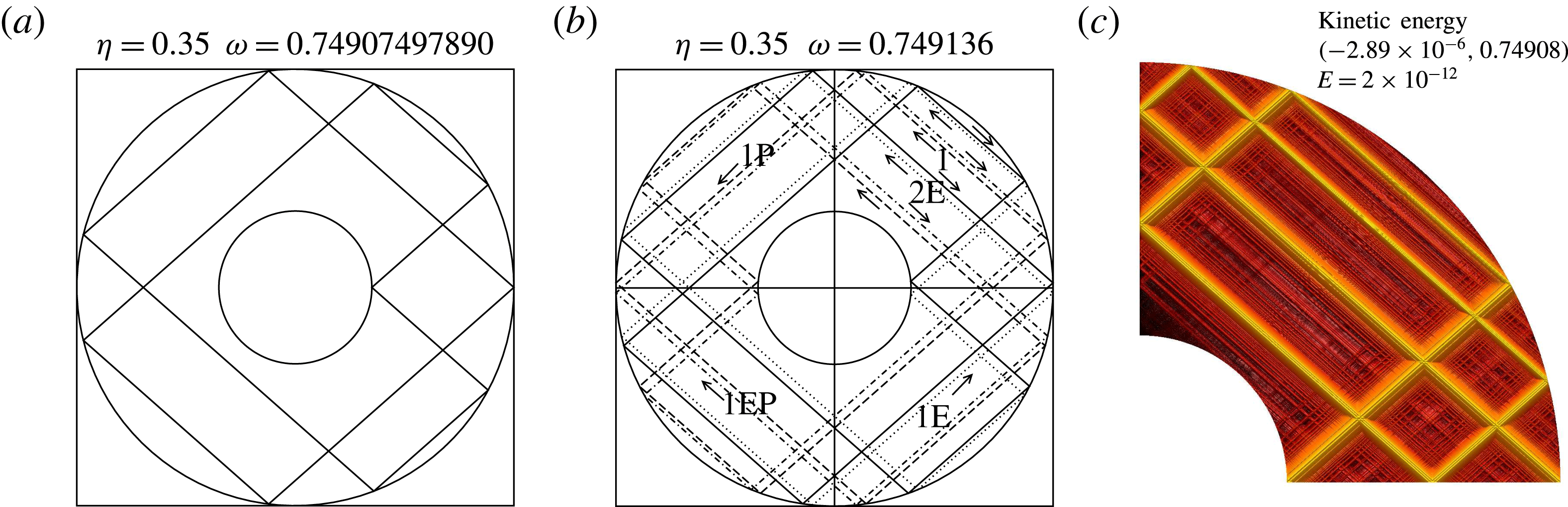
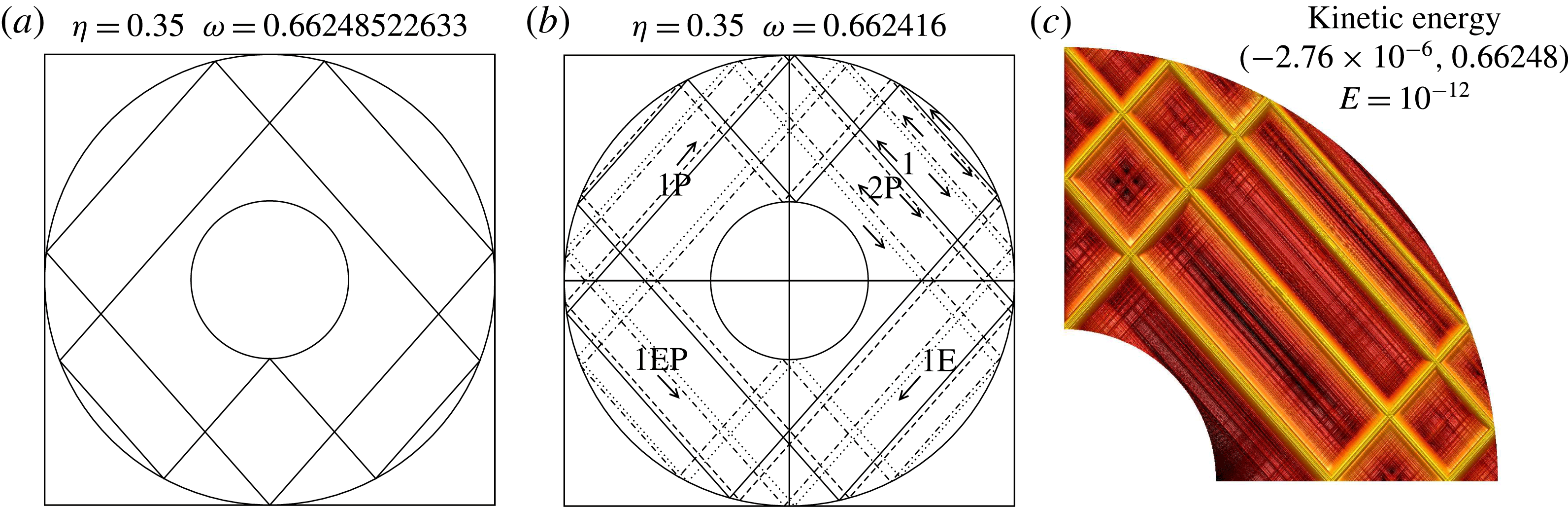
indeed gives a periodic orbit whatever the radius of the inner shell. As shown in Rieutord et al. (Reference Rieutord, Georgeot and Valdettaro2001), other periodic orbits are possible if the radius of the inner core is small enough. In figure 16 we show the neat transformation of the spectrum around
 $\unicode[STIX]{x1D714}=\sin (\unicode[STIX]{x03C0}/8)$
when the radius of the inner core is decreased from 0.35 to 0.20. When
 $\unicode[STIX]{x1D702}=0.35$
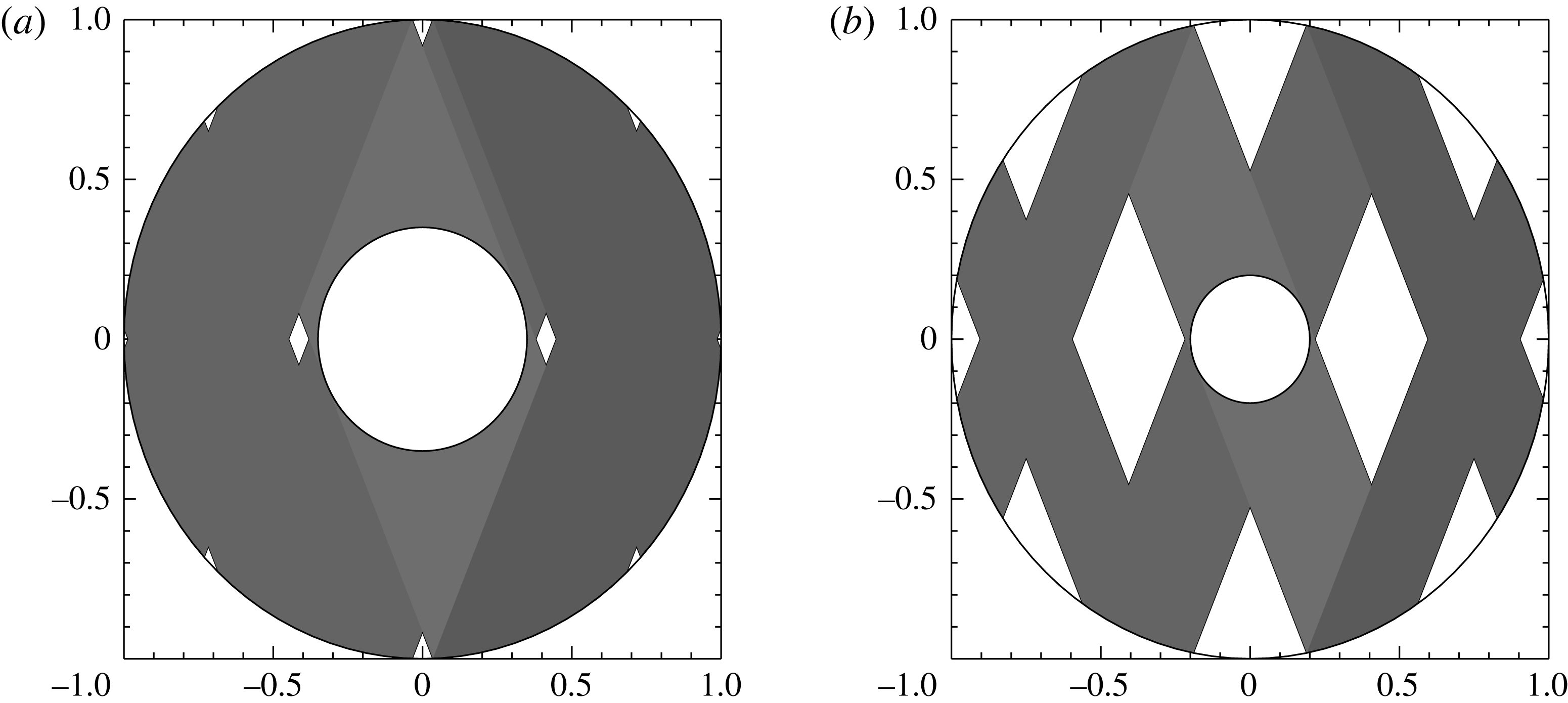
periodic orbits are possible, but mainly in the shadow path of the core (see figure 17). When the core is smaller, periodic orbits similar to those of the full sphere (i.e. that never hit the inner boundary) have a larger phase space that allows modes with larger scales to exist, and we recover a spectrum structure that is similar to that of the full sphere (compare figures 16(b) and 14). When
 $\unicode[STIX]{x1D702}=0.35$
, it is likely that a similar structure exists, but at scales that are not reachable numerically.
The quasi-regular nature of the modes around frequencies
 $\sin (p\unicode[STIX]{x03C0}/q)$
that are allowed by the size of the core is however not systematic. While investigating the case of
 $\unicode[STIX]{x1D714}=\sin (\unicode[STIX]{x03C0}/6)$
, which is associated with periodic orbits when
 $\unicode[STIX]{x1D702}\leqslant 0.5$
, we found that no regular quantization occurs if
 $\unicode[STIX]{x1D702}=0.35$
but also if
 $\unicode[STIX]{x1D702}=0.20$
. Inspection of the eigenmodes shows that the critical latitude singularity on the inner sphere is excited, hence inserting new scales in the eigenfunctions and precluding any regular behaviour as well as simple quantization rules. The reason why this occurs for this periodic orbit and not the others is not clear.
Shadow of the core when
 $\unicode[STIX]{x1D714}=\sin (\unicode[STIX]{x03C0}/8)$
for
 $\unicode[STIX]{x1D702}=0.35$
(a) and
 $\unicode[STIX]{x1D702}=0.2$
(b).

4 Analysis of attractor modes
We now analyse the dynamics of the flows that structures the shear layers looping around the attractors.
4.1 Summary of numerical results
The first hint given by the numerical solutions is the law (3.2) governing the eigenvalues associated with attractor modes. From this law we note that the frequency shift of the modes with respect to the asymptotic frequency
 $\unicode[STIX]{x1D714}_{0}$
is
 $\text{Im}(\unicode[STIX]{x1D706}-\text{i}\unicode[STIX]{x1D714}_{0})=O(E^{1/3})$
. Since the distance between the actual attractor and the asymptotic one varies like
 $\sqrt{|\unicode[STIX]{x1D714}-\unicode[STIX]{x1D714}_{0}|}$
(Rieutord et al.
Reference Rieutord, Georgeot and Valdettaro2001), we deduce that this distance scales like
 $E^{1/6}$
. Besides, as already shown by Kerswell (Reference Kerswell1995), the scale
 $E^{1/3}$
turns out to be the smallest scale of detached shear layers. However, Rieutord & Valdettaro (Reference Rieutord and Valdettaro1997) also noticed that some shear layers display a thickness scaling with
 $E^{1/4}$
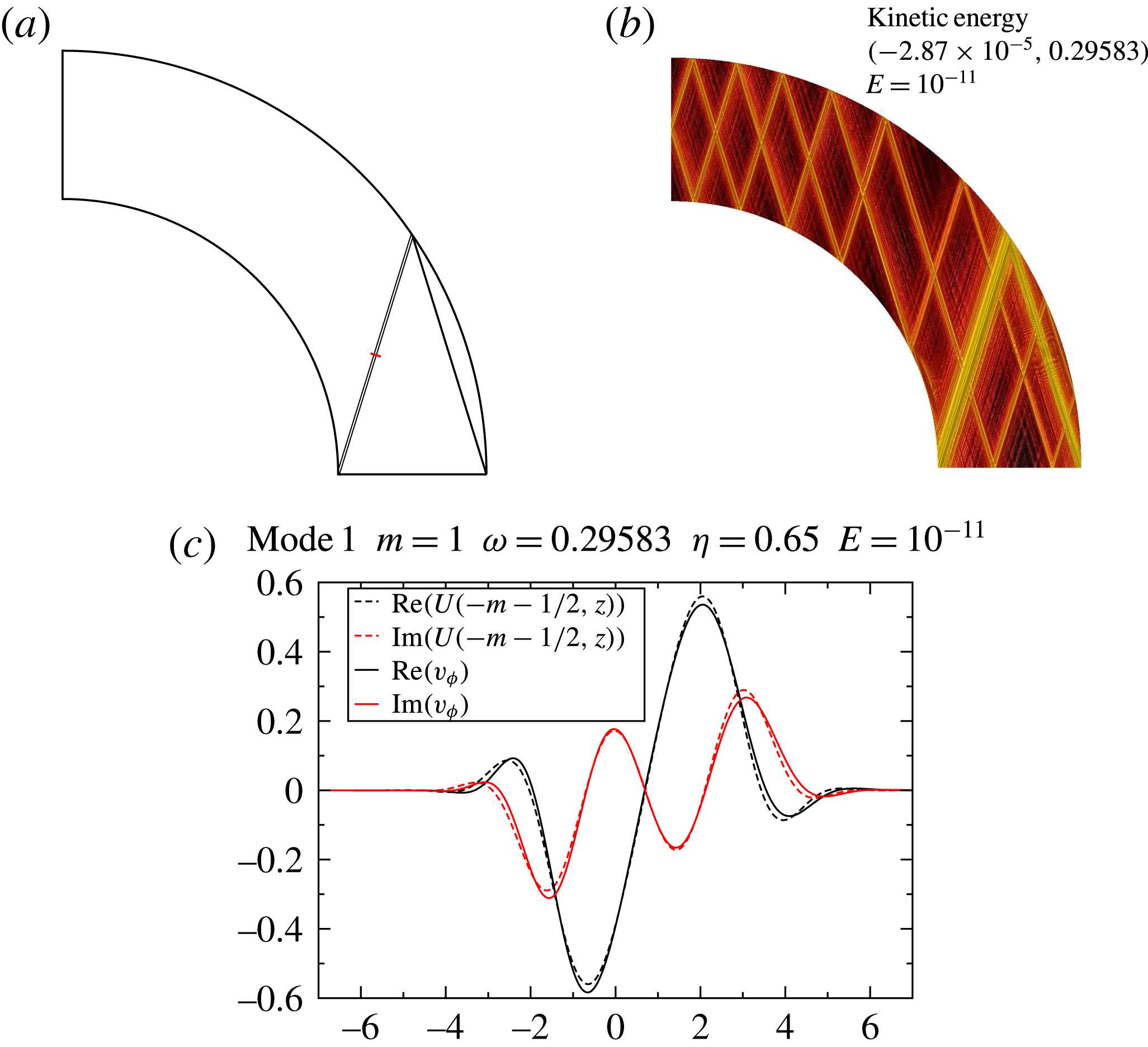
. We can illustrate the presence of these three scales using modes associated with the asymptotic attractor whose frequency is
 $\unicode[STIX]{x1D714}_{0}=0.782$
(when
 $\unicode[STIX]{x1D702}=0.35$
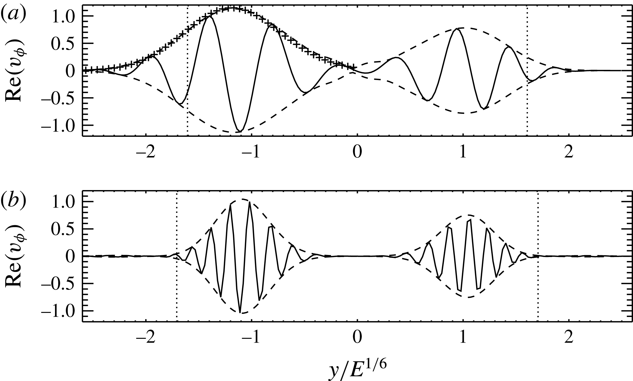
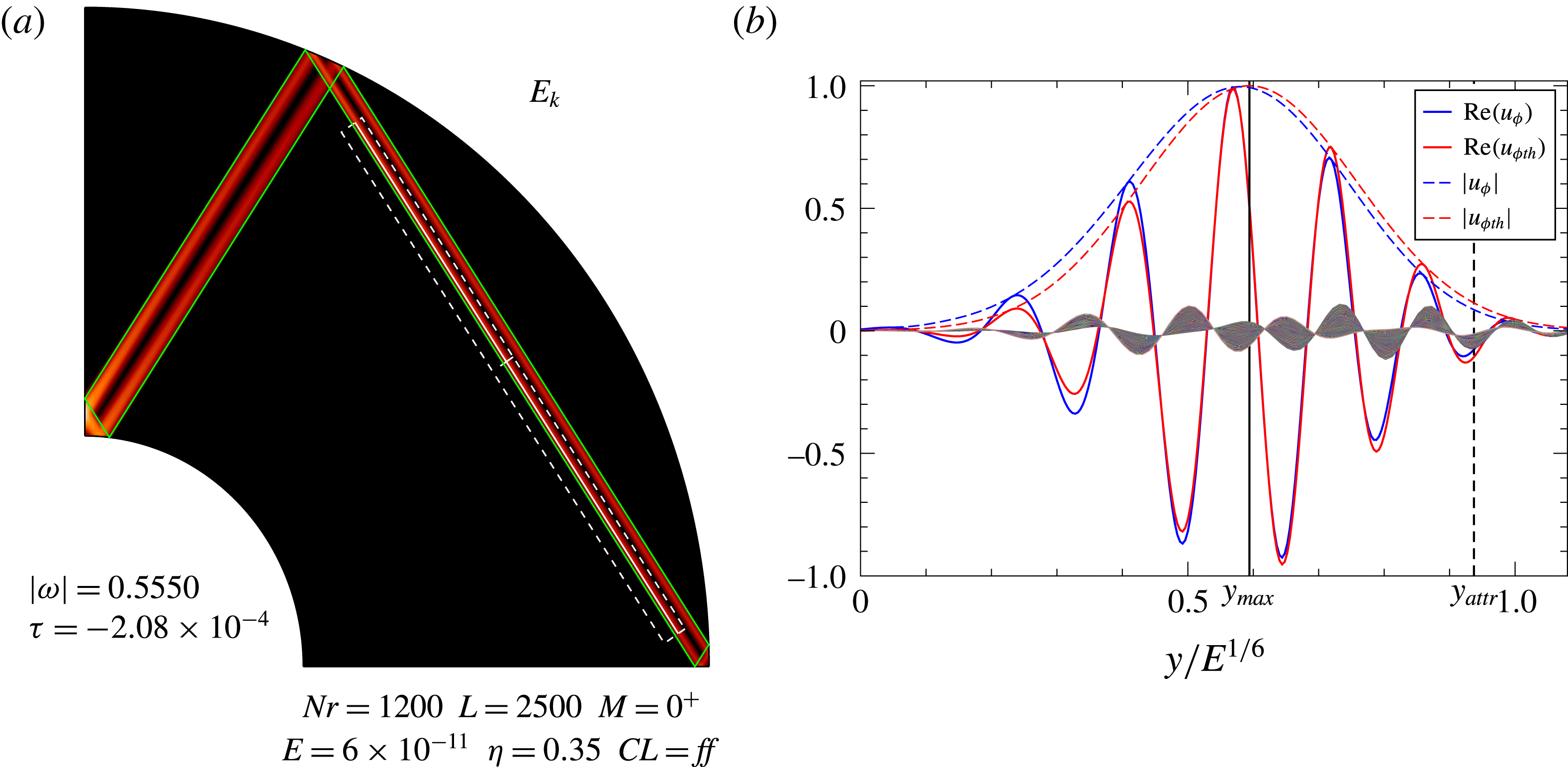
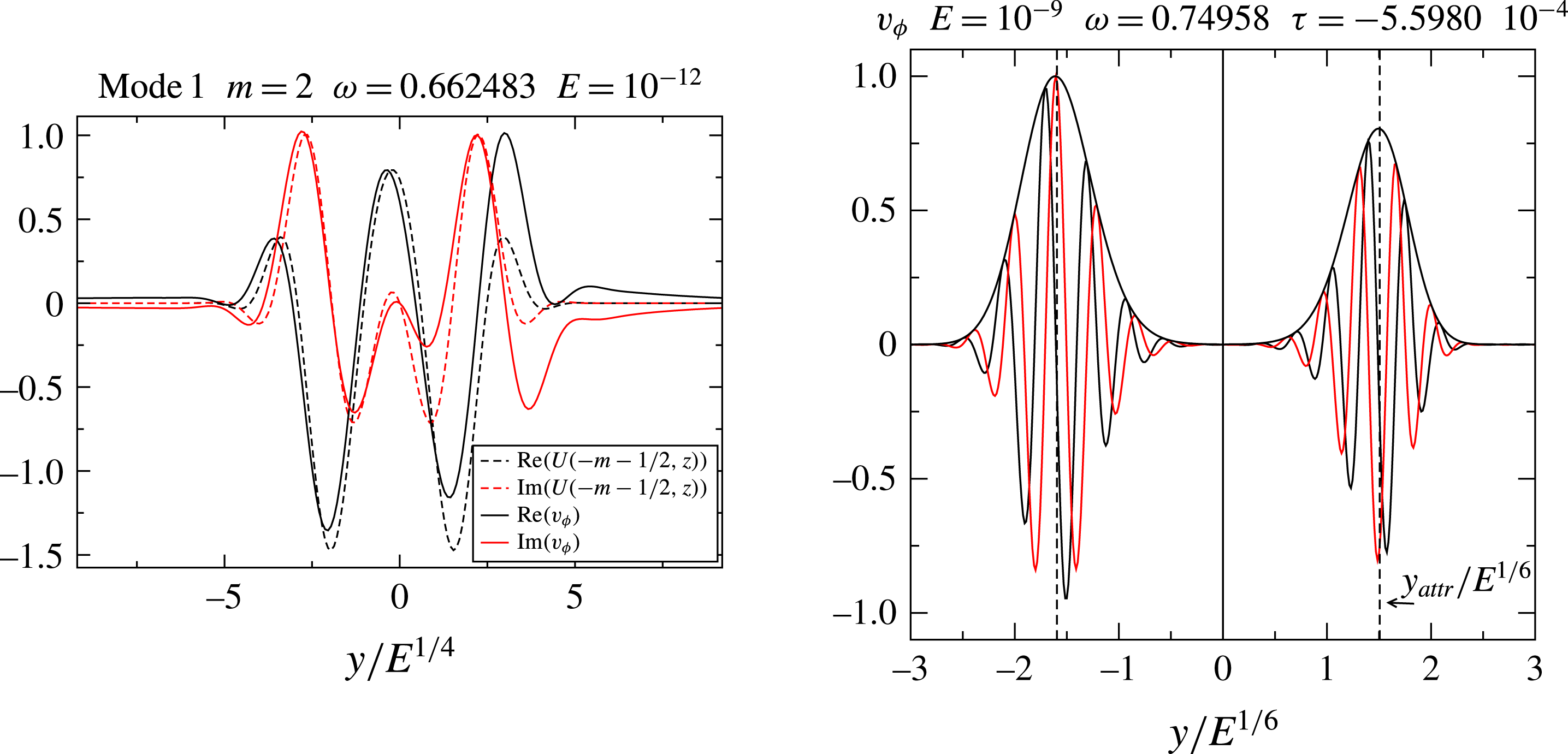
). Figure 2(a) displays the shape of the least-damped mode associated with this attractor. In figure 18 we show the variations of the amplitude of the velocity component
 $u_{\unicode[STIX]{x1D711}}$
in the transverse direction of the shear layer. The three scales are clearly showing up. Indeed, taking the origin of the coordinate at the asymptotic attractor, and rescaling the coordinate with
 $E^{1/6}$
, we see that the position of the maximum does not change when the Ekman number drops from
 $10^{-8}$
to
 $10^{-11}$
. In (a), we note that the rescaled envelope of the
 $E=10^{-11}$
-solution perfectly matches the
 $E=10^{-8}$
-envelope, hence giving evidence that the
 $E^{1/4}$
scale indeed determines the width of the wave packet. Finally, the ratio of the wavelength, rescaled by
 $E^{1/6}$
, is
 $\simeq 3.12$
, not far from the expected
 $\sqrt{10}\simeq 3.16$
if the wavelength scales as
 $E^{1/3}$
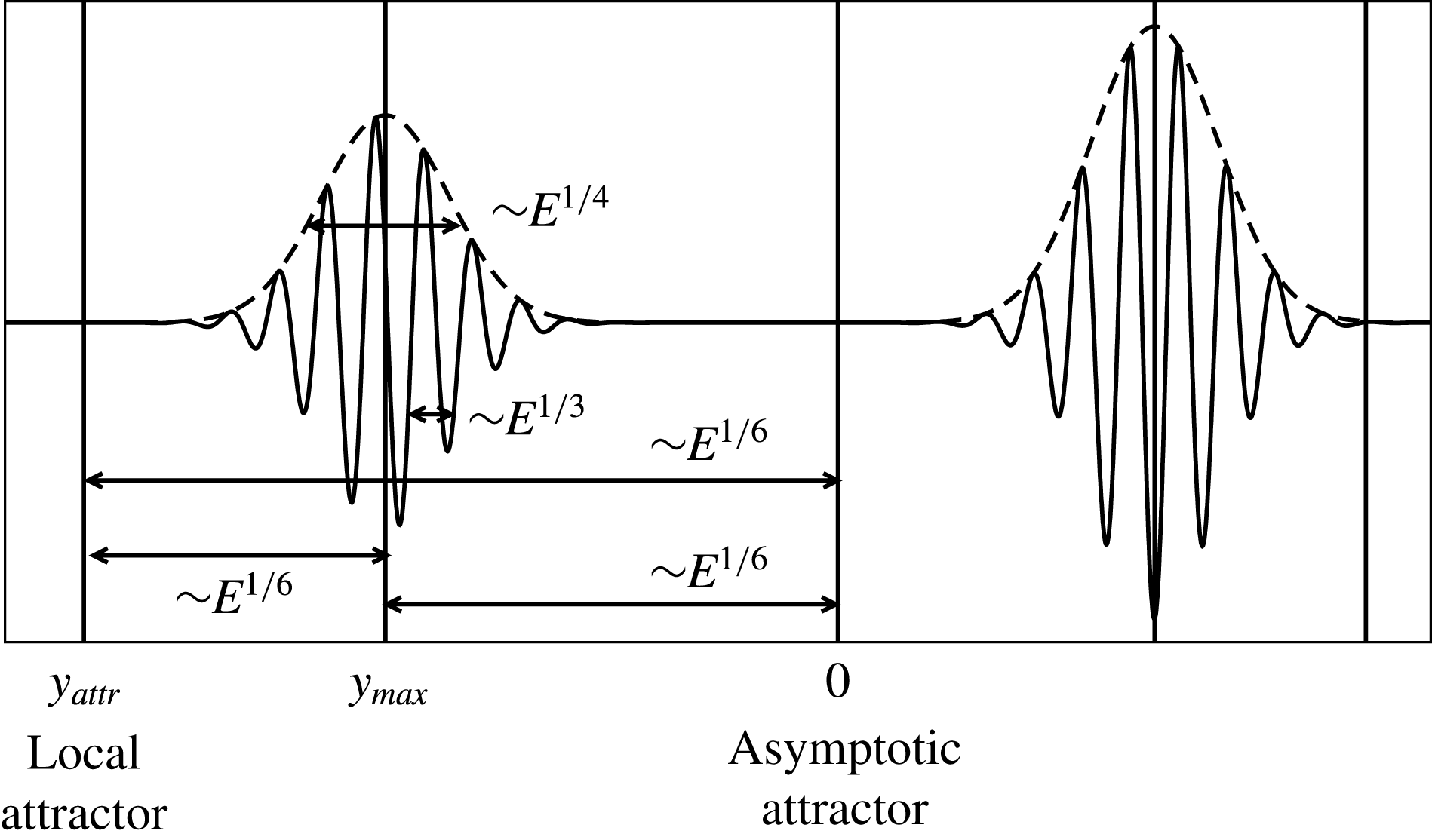
. Since the three scales also appear as such in other attractor modes, we shall assume that they are the scales controlling the dynamics of the shear layers associated with (at least some) attractor modes. Figure 19 schematically depicts the situation.
Cut through the shear layers of the least-damped mode associated with the attractor displayed in figure 2. (a)
 $E=10^{-8}$
. (b)
 $E=10^{-11}$
. The origin of the
 $y$
-coordinate is the position of the asymptotic attractor while the dotted vertical lines show the position of the actual attractor. The dashed curves show the envelope of the wave packet. In (a) the pluses show the rescaled envelope of the
 $E=10^{-11}$
-solution assuming an
 $E^{1/4}$
-scaling law for the width of the envelope.

Schematic view of the cut through shear layers looping around the attractors, showing the three scales involved:
 $E^{1/6}$
is the scale governing the distance among local attractor, asymptotic attractor and the shear layer.
 $E^{1/4}$
gives the extension of the shear layer.
 $E^{1/3}$
is the wavelength of the oscillations inside the shear layer. Note that both the local attractor and the asymptotic attractor are positioned (asymptotically as
 $E\rightarrow 0$
) outside the shear layer.

4.2 The reduced problem
To begin with we recall that system (2.1) can be cast into a single equation for the pressure perturbation, namely
 $$\begin{eqnarray}(\unicode[STIX]{x1D706}-E\unicode[STIX]{x0394})^{2}\unicode[STIX]{x0394}P+\frac{\unicode[STIX]{x2202}^{2}P}{\unicode[STIX]{x2202}z^{2}}=0,\end{eqnarray}$$
where we assumed solutions of the form
 $$\begin{eqnarray}P(\boldsymbol{r},t)=P(\boldsymbol{r})\text{e}^{\unicode[STIX]{x1D706}t}\end{eqnarray}$$
and where
 $\unicode[STIX]{x1D706}=\unicode[STIX]{x1D70F}+\text{i}\unicode[STIX]{x1D714}$
is the complex frequency.
 $\unicode[STIX]{x1D70F}$
is the damping rate and
 $\unicode[STIX]{x1D714}$
the real frequency of the mode. Equation (4.1) reduces to the Poincaré equation when the Ekman number
 $E$
is set to zero.
As observed by Rieutord & Valdettaro (Reference Rieutord and Valdettaro1997), shear layers built on attractors have an (inviscid) singularity on the rotation axis generating a divergence in
 $s^{-1/2}$
, where
 $s$
is the radial cylindrical coordinate. We remove this divergence by setting
 $P=ps^{-1/2}$
. Thus doing, we rewrite (4.1) as
 $$\begin{eqnarray}(\unicode[STIX]{x1D706}-E\unicode[STIX]{x0394}^{\prime })^{2}\unicode[STIX]{x0394}^{\prime }p+\frac{\unicode[STIX]{x2202}^{2}p}{\unicode[STIX]{x2202}z^{2}}=0,\end{eqnarray}$$
with
 $$\begin{eqnarray}\unicode[STIX]{x0394}^{\prime }={\displaystyle \frac{\unicode[STIX]{x2202}^{2}}{\unicode[STIX]{x2202}s^{2}}}+{\displaystyle \frac{\unicode[STIX]{x2202}^{2}}{\unicode[STIX]{x2202}z^{2}}}+{\displaystyle \frac{1}{4s^{2}}}.\end{eqnarray}$$
We also use coordinates parallel
 $x$
and perpendicular
 $y$
to the shear layer/attractor branch such that
 $$\begin{eqnarray}x=\unicode[STIX]{x1D6FC}z+\unicode[STIX]{x1D714}s,\quad y=\unicode[STIX]{x1D714}z-\unicode[STIX]{x1D6FC}s,\end{eqnarray}$$
with
 $\unicode[STIX]{x1D6FC}=\sqrt{1-\unicode[STIX]{x1D714}^{2}}$
. This implies that
 $$\begin{eqnarray}{\displaystyle \frac{\unicode[STIX]{x2202}}{\unicode[STIX]{x2202}s}}=\unicode[STIX]{x1D714}{\displaystyle \frac{\unicode[STIX]{x2202}}{\unicode[STIX]{x2202}x}}-\unicode[STIX]{x1D6FC}{\displaystyle \frac{\unicode[STIX]{x2202}}{\unicode[STIX]{x2202}y}},\quad {\displaystyle \frac{\unicode[STIX]{x2202}}{\unicode[STIX]{x2202}z}}=\unicode[STIX]{x1D6FC}{\displaystyle \frac{\unicode[STIX]{x2202}}{\unicode[STIX]{x2202}x}}+\unicode[STIX]{x1D714}{\displaystyle \frac{\unicode[STIX]{x2202}}{\unicode[STIX]{x2202}y}},\quad {\displaystyle \frac{\unicode[STIX]{x2202}^{2}}{\unicode[STIX]{x2202}z^{2}}}=\unicode[STIX]{x1D6FC}^{2}{\displaystyle \frac{\unicode[STIX]{x2202}^{2}}{\unicode[STIX]{x2202}x^{2}}}+\unicode[STIX]{x1D714}^{2}{\displaystyle \frac{\unicode[STIX]{x2202}^{2}}{\unicode[STIX]{x2202}y^{2}}}+2\unicode[STIX]{x1D6FC}\unicode[STIX]{x1D714}{\displaystyle \frac{\unicode[STIX]{x2202}^{2}}{\unicode[STIX]{x2202}x\unicode[STIX]{x2202}y}}.\end{eqnarray}$$
From the numerical solutions we find that (see (3.2))
 $$\begin{eqnarray}\unicode[STIX]{x1D706}=\text{i}\unicode[STIX]{x1D714}_{0}+\unicode[STIX]{x1D706}_{1}E^{1/3}+\unicode[STIX]{x1D706}_{2}E^{1/2}+\cdots \,.\end{eqnarray}$$
The numerical solutions have also shown the importance of three non-dimensional scales:
 $E^{1/3}$
,
 $E^{1/4}$
and
 $E^{1/6}$
. If we select the smallest scale
 $E^{1/3}$
and consider the dominating terms, the full equation (4.3) can be reduced to a simpler equation, which reads:
 $$\begin{eqnarray}\unicode[STIX]{x1D6FC}_{0}{\displaystyle \frac{\unicode[STIX]{x2202}p}{\unicode[STIX]{x2202}x}}=\text{i}E{\displaystyle \frac{\unicode[STIX]{x2202}^{3}p}{\unicode[STIX]{x2202}y^{3}}}-\text{i}\unicode[STIX]{x1D70F}{\displaystyle \frac{\unicode[STIX]{x2202}p}{\unicode[STIX]{x2202}y}}\end{eqnarray}$$
and which we shall call the reduced problem. Its derivation is given in appendix A. We now analyse this new and simpler but still very rich equation. We remark that this equation is the same as the one we obtained for the slender torus considered in Rieutord et al. (Reference Rieutord, Valdettaro and Georgeot2002). The geometry in the meridional section is also the same. The only difference between the two cases is that in the spherical geometry the reflection on the rotation axis produces a variation in the solution: We show in appendix B that if viscosity is neglected each reflection produces a factor
 $-\text{i}$
in the eigenfunction. This effect is not present in the toroidal configuration, as there is no axial singularity there. Viscosity may actually alter the phase shift due to axis reflection, but we leave this possible effect to future investigations. Finally, we may note that attractors bouncing
 $K$
times impose a factor
 $(-\text{i})^{K}$
in the solution, but this factor reduces to unity if
 $K=4n$
. As we shall see below, the analytical two-dimensional solutions obtained for the slender torus can offer a very good approximation to the eigenmodes made of shear layers bouncing
 $4n$
times on the rotation axis, even in a thick shell.
4.3 Local dynamics of shear layers
Let us first assume that the shear layers are formed by the product of a fast oscillating wave of wavenumber scaling as
 $O(E^{-1/3})$
and a wide
 $O(E^{1/4})$
envelope. It is convenient to set
 $p=\text{e}^{\unicode[STIX]{x1D713}}$
and to work with
 $\unicode[STIX]{x1D713}$
. The equation for
 $\unicode[STIX]{x1D713}$
is:
 $$\begin{eqnarray}\unicode[STIX]{x1D6FC}_{0}{\displaystyle \frac{\unicode[STIX]{x2202}\unicode[STIX]{x1D713}}{\unicode[STIX]{x2202}x}}=\text{i}E\left[\frac{\unicode[STIX]{x2202}^{3}\unicode[STIX]{x1D713}}{\unicode[STIX]{x2202}y^{3}}+3\frac{\unicode[STIX]{x2202}^{2}\unicode[STIX]{x1D713}}{\unicode[STIX]{x2202}y^{2}}\frac{\unicode[STIX]{x2202}\unicode[STIX]{x1D713}}{\unicode[STIX]{x2202}y}+\left(\frac{\unicode[STIX]{x2202}\unicode[STIX]{x1D713}}{\unicode[STIX]{x2202}y}\right)^{3}\right]+\text{i}E^{1/3}|\hat{\unicode[STIX]{x1D70F}}|\frac{\unicode[STIX]{x2202}\unicode[STIX]{x1D713}}{\unicode[STIX]{x2202}y},\end{eqnarray}$$
where we have set
 $|\hat{\unicode[STIX]{x1D70F}}|=-\unicode[STIX]{x1D70F}E^{-1/3}$
, hence
 $|\hat{\unicode[STIX]{x1D70F}}|\sim O(E^{0})$
. We remark that an exact solution to this equation is the linear function:
 $$\begin{eqnarray}\unicode[STIX]{x1D713}(x,y)={\displaystyle \frac{q^{3}-|\hat{\unicode[STIX]{x1D70F}}|q}{\unicode[STIX]{x1D6FC}_{0}}}x+E^{-1/3}\text{i}qy,\end{eqnarray}$$
where
 $q$
is any complex constant. We shall make the assumption that
 $q$
is real, so that (4.10) describes a wave with spatial frequency
 $qE^{-1/3}/2\unicode[STIX]{x03C0}$
in the
 $y$
direction and exponential variation in the
 $x$
direction. This function accounts for the
 $E^{1/3}$
oscillations of the shear layers observed numerically. The foregoing solution is not localized and we therefore need to seek for the envelope of the wave that keeps it close to the attractor. Recalling that
 $p=\text{e}^{\unicode[STIX]{x1D713}}$
, we now set
 $$\begin{eqnarray}\unicode[STIX]{x1D713}={\displaystyle \frac{q^{3}-|\hat{\unicode[STIX]{x1D70F}}|q}{\unicode[STIX]{x1D6FC}_{0}}}x+E^{-1/3}\text{i}qy+h(x,y)\end{eqnarray}$$
and we shall assume that
 $h\sim O(E^{0})$
,
 $(\unicode[STIX]{x2202}^{n}h/\unicode[STIX]{x2202}y^{n})\sim E^{-n/4}$
,
 $(\unicode[STIX]{x2202}h/\unicode[STIX]{x2202}x)\sim E^{1/12}$
. We insert this expression into (4.9). To leading order, that is
 $O(E^{1/12})$
, we get the following equation for
 $h$
:
 $$\begin{eqnarray}\unicode[STIX]{x1D6FC}_{0}{\displaystyle \frac{\unicode[STIX]{x2202}h}{\unicode[STIX]{x2202}x}}=\text{i}E^{1/3}(|\hat{\unicode[STIX]{x1D70F}}|-3q^{2}){\displaystyle \frac{\unicode[STIX]{x2202}h}{\unicode[STIX]{x2202}y}}.\end{eqnarray}$$
This first-order linear partial differential equation has the following general solution:
 $$\begin{eqnarray}h(x,y)=f(Z),\quad \text{with }Z={\displaystyle \frac{\text{i}(|\hat{\unicode[STIX]{x1D70F}}|-3q^{2})}{\unicode[STIX]{x1D6FC}_{0}}}E^{1/12}x+E^{-1/4}y,\end{eqnarray}$$
where
 $f(Z)$
is an arbitrary function. Numerical solutions suggest that the envelope is a Gaussian, which would be the case if
 $f(Z)=-aZ^{2}$
for some complex coefficient
 $a$
with a positive real part. We shall prove in the following that
 $f(Z)$
has indeed this shape and we shall provide the expression of
 $a$
as a function of the eigenvalue and of the geometrical parameters of the attractor (see (4.36)).
4.3.1 Viscous evolution along a characteristic path
We now wish to obtain the variation of the solution after travelling one complete loop along the attractor. After reflection on a boundary,
 $p$
is rescaled as
 $$\begin{eqnarray}p_{n}(x_{n},y)=K_{n}p\left(x_{1},{\displaystyle \frac{y}{K_{n}}}\right),\end{eqnarray}$$
where
 $K_{n}$
are products of contraction/dilation coefficients arising from the reflections at the boundaries. They are the same as those of Rieutord et al. (Reference Rieutord, Valdettaro and Georgeot2002). (Note that there is a misprint on page 354 of Rieutord et al. (Reference Rieutord, Valdettaro and Georgeot2002): the third formula of that page should read like (4.14) instead of having
 $K_{n}$
at the denominator twice). Therefore the spatial frequency
 $q$
is multiplied at each reflection by the factor
 $1/K_{n}$
. Taking the first branch as the reference, we set
 $K_{1}=1$
. The variation of the
 $E^{1/3}$
part of the solution (4.10) after travelling over the length
 $\unicode[STIX]{x1D6FF}x=\ell _{n}$
on the branch
 $n$
is exactly:
 $$\begin{eqnarray}\unicode[STIX]{x1D6FF}\unicode[STIX]{x1D713}_{n}={\displaystyle \frac{(q/K_{n})^{3}-|\hat{\unicode[STIX]{x1D70F}}|q/K_{n}}{\unicode[STIX]{x1D6FC}_{0}}}\ell _{n}.\end{eqnarray}$$
Since
 $h$
varies by a small
 $O(E^{1/12})$
amount over each branch, we can use the same procedure as in §3.2 of Rieutord et al. (Reference Rieutord, Valdettaro and Georgeot2002) to determine its variation after one loop. On branch
 $n$
we have:
 $$\begin{eqnarray}\displaystyle \unicode[STIX]{x1D6FF}h_{n} & = & \displaystyle h_{n}(x_{n}+\ell _{n},y)-h_{n}(x_{n},y)\simeq \frac{\unicode[STIX]{x2202}h}{\unicode[STIX]{x2202}x}\bigg|_{x_{n},y}\ell _{n}\nonumber\\ \displaystyle & = & \displaystyle {\displaystyle \frac{\text{i}E^{1/3}}{\unicode[STIX]{x1D6FC}_{0}}}\left(|\hat{\unicode[STIX]{x1D70F}}|-{\displaystyle \frac{3q^{2}}{K_{n}^{2}}}\right)\frac{\unicode[STIX]{x2202}h(x_{1},y/K_{n})}{\unicode[STIX]{x2202}y}\ell _{n}.\end{eqnarray}$$
Since the functions
 $h_{n}$
are the same on every branch up to a scale factor
 $K_{n}$
, we can write (4.16) as
 $$\begin{eqnarray}\displaystyle \unicode[STIX]{x1D6FF}h_{n} & = & \displaystyle {\displaystyle \frac{\text{i}E^{1/3}}{\unicode[STIX]{x1D6FC}_{0}}}\left({\displaystyle \frac{|\hat{\unicode[STIX]{x1D70F}}|}{K_{n}}}-{\displaystyle \frac{3q^{2}}{K_{n}^{3}}}\right)\frac{\unicode[STIX]{x2202}h(x_{1},y/K_{n})}{\unicode[STIX]{x2202}(y/K_{n})}\ell _{n}\nonumber\\ \displaystyle & = & \displaystyle {\displaystyle \frac{\text{i}E^{1/3}}{\unicode[STIX]{x1D6FC}_{0}}}\left({\displaystyle \frac{|\hat{\unicode[STIX]{x1D70F}}|}{K_{n}}}-{\displaystyle \frac{3q^{2}}{K_{n}^{3}}}\right)\frac{\unicode[STIX]{x2202}h(x_{1},y)}{\unicode[STIX]{x2202}y}\ell _{n},\end{eqnarray}$$
where all the derivatives are taken on the first branch.
Finally we have to take into account the variations due to the reflections on the rotation axis: as we show in appendix B, each reflection introduces a factor
 $-\text{i}$
in the eigenfunction; therefore
 $\unicode[STIX]{x1D713}$
is shifted by
 $-\text{i}\unicode[STIX]{x03C0}/2$
at each reflection.
Summing up all the contributions of the perturbations arising from all the branches of the attractor we get:
 $$\begin{eqnarray}\unicode[STIX]{x1D6FF}\unicode[STIX]{x1D713}^{propag.}=\underbrace{-{\displaystyle \frac{\text{i}K\unicode[STIX]{x03C0}}{2}}+{\displaystyle \frac{Aq^{3}-B|\hat{\unicode[STIX]{x1D70F}}|q}{\unicode[STIX]{x1D6FC}_{0}}}}_{O(E^{0})}+\underbrace{{\displaystyle \frac{\text{i}E^{1/3}}{\unicode[STIX]{x1D6FC}_{0}}}\left(B|\hat{\unicode[STIX]{x1D70F}}|-3Aq^{2}\right){\displaystyle \frac{\unicode[STIX]{x2202}h}{\unicode[STIX]{x2202}y}}}_{O(E^{1/12})},\end{eqnarray}$$
where
 $K$
is the total number of reflections on the axis, and
 $$\begin{eqnarray}A=\mathop{\sum }_{n}{\displaystyle \frac{\ell _{n}}{K_{n}^{3}}},\quad B=\mathop{\sum }_{n}{\displaystyle \frac{\ell _{n}}{K_{n}}}.\end{eqnarray}$$
We remark that the values of
 $A$
and
 $B$
depend on the branch of the attractor that is chosen as the first branch. The quantity
 $d=B^{3}/A$
however does not change. Expression (4.18) gives, terms up to order
 $E^{1/12}$
, the variation of the perturbation due to viscosity when the wave has the
 $E^{1/3}$
and
 $E^{1/4}$
scales. Except for the reflections on the boundaries, which rescale the width of the layer by some factor of order unity, the foregoing expression is just an approximate solution of (4.8). We now need to take into account the fact that the perturbation is not strictly on the attractor and therefore that after one loop the place where we measure the variation
 $\unicode[STIX]{x1D6FF}\unicode[STIX]{x1D713}$
is not the same as the initial one: it has been shifted by a small amount controlled by the mapping. Indeed, the only point that comes back to the same place is the one on the attractor.
4.4 The part played by the mapping
To take into account the shift induced by the mapping, we use the same procedure as the one devised in Rieutord et al. (Reference Rieutord, Valdettaro and Georgeot2002). Indeed, the mapping drawn by characteristics in the meridional plane of the spherical shell is the same as the one of the slender torus used in Rieutord et al. (Reference Rieutord, Valdettaro and Georgeot2002).
Here too, we shall work with the associated critical latitude
 $\unicode[STIX]{x1D703}^{c}=\arcsin \unicode[STIX]{x1D714}$
, rather than with the frequency
 $\unicode[STIX]{x1D714}$
. Thus,
 $\unicode[STIX]{x1D703}_{0}^{c}$
designates the critical latitude associated with the frequency
 $\unicode[STIX]{x1D714}_{0}$
of the asymptotic attractor.
We introduce the mapping as the function
 $f(\unicode[STIX]{x1D719},\unicode[STIX]{x1D703}^{c})$
that associates the latitude
 $\unicode[STIX]{x1D719}$
, where the characteristic bounces on the inner or outer boundary, with the latitude of its image after one loop along the attractor. The
 $y$
-coordinate introduced in (4.8) is related to the latitude
 $\unicode[STIX]{x1D719}$
by
 $$\begin{eqnarray}y=p(\unicode[STIX]{x1D719}-\unicode[STIX]{x1D719}_{0})\quad \text{with }p=r\sin (\unicode[STIX]{x1D719}_{0}\pm \unicode[STIX]{x1D703}_{0}^{c}),\end{eqnarray}$$
where
 $\unicode[STIX]{x1D719}_{0}$
is the latitude of the reflection point of the asymptotic attractor and
 $r$
is the radius of the reflecting sphere (either
 $\unicode[STIX]{x1D702}$
or
 $1$
). The
 $\pm$
sign denotes the sign of the slope of the chosen characteristic. Finally, we note that
 $\unicode[STIX]{x1D719}_{0}$
is also the fixed point of the mapping when
 $\unicode[STIX]{x1D703}^{c}=\unicode[STIX]{x1D703}_{0}^{c}$
.
Since the mapping just displaces the points, its action on the velocity field complies with
 $$\begin{eqnarray}u(f(y,\unicode[STIX]{x1D703}^{c}),\unicode[STIX]{x1D703}^{c})\,\text{d}f=u^{propag.}(y,\unicode[STIX]{x1D703}^{c})\,\text{d}y,\end{eqnarray}$$
where
 $u^{propag.}(y,\unicode[STIX]{x1D703}^{c})$
is the flow field obtained after propagation along the map with starting point
 $(x_{1},y)$
. Here and in the following
 $x_{1}$
will be omitted.
 $u$
can be understood as the toroidal component of velocity multiplied by the square root of the distance to the rotation axis
 $s^{1/2}$
. It admits the same evolution equation (4.8) as the reduced pressure and thus has the same solution.
In order to find the displacement due to the mapping we make a Taylor expansion of the mapping around the fixed point of the asymptotic attractor, namely around
 $\unicode[STIX]{x1D719}=\unicode[STIX]{x1D719}_{0}$
(that is
 $y=0$
) and
 $\unicode[STIX]{x1D703}^{c}=\unicode[STIX]{x1D703}_{0}^{c}$
. Following the appendix of Rieutord et al. (Reference Rieutord, Georgeot and Valdettaro2001), we get:
 $$\begin{eqnarray}f(\unicode[STIX]{x1D719},\unicode[STIX]{x1D703}^{c})=\unicode[STIX]{x1D719}+f_{01}\unicode[STIX]{x1D6FF}\unicode[STIX]{x1D703}+{\textstyle \frac{1}{2}}f_{20}(\unicode[STIX]{x1D719}-\unicode[STIX]{x1D719}_{0})^{2}+{\textstyle \frac{1}{2}}f_{02}\unicode[STIX]{x1D6FF}\unicode[STIX]{x1D703}^{2}+f_{11}\unicode[STIX]{x1D6FF}\unicode[STIX]{x1D703}(\unicode[STIX]{x1D719}-\unicode[STIX]{x1D719}_{0})+\cdots \,,\end{eqnarray}$$
where
 $\unicode[STIX]{x1D6FF}\unicode[STIX]{x1D703}=\unicode[STIX]{x1D703}^{c}-\unicode[STIX]{x1D703}_{0}^{c}$
. We defined
 $$\begin{eqnarray}f_{ij}\equiv \left.{\displaystyle \frac{\unicode[STIX]{x2202}^{i+j}f}{\unicode[STIX]{x2202}\unicode[STIX]{x1D719}^{i}\unicode[STIX]{x2202}\unicode[STIX]{x1D703}^{j}}}\right|_{\unicode[STIX]{x1D719}_{0},\unicode[STIX]{x1D703}_{0}}.\end{eqnarray}$$
We recall that numerical solutions say that
 $\unicode[STIX]{x1D6FF}\unicode[STIX]{x1D703}=O(E^{1/3})$
and
 $\unicode[STIX]{x1D719}-\unicode[STIX]{x1D719}_{0}=O(E^{1/6})$
. The foregoing expression of
 $f$
leads to
 $$\begin{eqnarray}f(y,\unicode[STIX]{x1D703})=p(f-\unicode[STIX]{x1D719}_{0})=y+pf_{01}\unicode[STIX]{x1D6FF}\unicode[STIX]{x1D703}+{\displaystyle \frac{f_{20}}{2p}}y^{2}+\cdots \,.\end{eqnarray}$$
It is convenient to shift the
 $y$
coordinate and develop around
 $\bar{y}=y-y_{max}$
, where
 $y_{max}$
is the position where the wave packet amplitude is maximum (see figure 19). We shall assume
 $\bar{y}\sim O(E^{1/4})$
and we shall drop all contributions smaller than
 $O(E^{5/12})$
. We thus have:
 $$\begin{eqnarray}f(y,\unicode[STIX]{x1D706}^{c})=\underbrace{y_{max}}_{E^{2/12}}+\underbrace{\bar{y}}_{E^{3/12}}+\underbrace{pf_{01}\unicode[STIX]{x1D6FF}\unicode[STIX]{x1D703}+{\displaystyle \frac{f_{20}}{2p}}y_{max}^{2}}_{E^{4/12}}+\underbrace{{\displaystyle \frac{f_{20}}{p}}y_{max}\bar{y}}_{E^{5/12}}+\cdots \,.\end{eqnarray}$$
We rewrite (4.21) in terms of the exponent
 $\unicode[STIX]{x1D713}$
:
 $$\begin{eqnarray}\text{e}^{\unicode[STIX]{x1D713}(f(y,\unicode[STIX]{x1D703}^{c}),\unicode[STIX]{x1D703}^{c})}\,\text{d}f=\text{e}^{\unicode[STIX]{x1D713}^{propag.}(y,\unicode[STIX]{x1D703}^{c})}\,\text{d}y.\end{eqnarray}$$
We remark that
 $$\begin{eqnarray}\left.{\displaystyle \frac{\text{d}f}{\text{d}y}}\right|_{\bar{y}=0}=1+{\displaystyle \frac{f_{20}}{p}}y_{max}+\cdots =\text{e}^{(f_{20}/p)y_{max}+\cdots },\end{eqnarray}$$
where
 $f_{20}y_{max}/p$
is of order
 $E^{1/6}$
. Therefore (4.26) is turned simply into:
 $$\begin{eqnarray}\unicode[STIX]{x1D713}(f(y,\unicode[STIX]{x1D703}^{c}),\unicode[STIX]{x1D703}^{c})=\unicode[STIX]{x1D713}^{propag.}(y,\unicode[STIX]{x1D703}^{c})-{\displaystyle \frac{f_{20}}{p}}y_{max}+\cdots \,.\end{eqnarray}$$
We evaluate separately the left-hand side and the right-hand side of (4.28). For the left-hand side we replace
 $\unicode[STIX]{x1D713}$
with (4.11):
 $$\begin{eqnarray}\displaystyle \unicode[STIX]{x1D713}(f(y,\unicode[STIX]{x1D703}^{c}),\unicode[STIX]{x1D703}^{c})= & & \displaystyle {\displaystyle \frac{q^{3}-|\hat{\unicode[STIX]{x1D70F}}|q}{\unicode[STIX]{x1D6FC}_{0}}}x_{1}+E^{-1/3}\text{i}q\left(y+pf_{01}\unicode[STIX]{x1D6FF}\unicode[STIX]{x1D703}+{\displaystyle \frac{f_{20}}{2p}}y_{max}^{2}+{\displaystyle \frac{f_{20}}{p}}y_{max}\bar{y}\right)\nonumber\\ \displaystyle & & \displaystyle +\,h(x_{1},y)+\left.\frac{\unicode[STIX]{x2202}h}{\unicode[STIX]{x2202}y}\right|_{y}\left(pf_{01}\unicode[STIX]{x1D6FF}\unicode[STIX]{x1D703}+{\displaystyle \frac{f_{20}}{2p}}y_{max}^{2}+{\displaystyle \frac{f_{20}}{p}}y_{max}\bar{y}\right)+\cdots \,.\end{eqnarray}$$
For the evaluation of the right-hand side we use (4.18):
 $$\begin{eqnarray}\displaystyle \hspace{-12.0pt} & & \displaystyle \unicode[STIX]{x1D713}^{propag.}(y,\unicode[STIX]{x1D703}^{c})=\unicode[STIX]{x1D713}(y,\unicode[STIX]{x1D703}^{c})+\unicode[STIX]{x1D6FF}\unicode[STIX]{x1D713}^{propag.}(y,\unicode[STIX]{x1D703}^{c})={\displaystyle \frac{q^{3}-|\hat{\unicode[STIX]{x1D70F}}|q}{\unicode[STIX]{x1D6FC}_{0}}}x_{1}\nonumber\\ \displaystyle \hspace{-12.0pt} & & \displaystyle \quad +\,E^{-1/3}\text{i}q(y_{max}+\bar{y})+h(x_{1},y)-{\displaystyle \frac{\text{i}K\unicode[STIX]{x03C0}}{2}}+{\displaystyle \frac{Aq^{3}-B|\hat{\unicode[STIX]{x1D70F}}|q}{\unicode[STIX]{x1D6FC}_{0}}}+{\displaystyle \frac{\text{i}E^{1/3}}{\unicode[STIX]{x1D6FC}_{0}}}(B|\hat{\unicode[STIX]{x1D70F}}|-3Aq^{2})\left.\frac{\unicode[STIX]{x2202}h}{\unicode[STIX]{x2202}y}\right|_{y}.\nonumber\\ \displaystyle & & \displaystyle\end{eqnarray}$$
We are ready to insert these expressions into (4.28); dropping all contributions smaller than
 $E^{1/12}$
we get:
 $$\begin{eqnarray}\displaystyle & & \displaystyle \underbrace{E^{-1/3}\text{i}q(pf_{01}\unicode[STIX]{x1D6FF}\unicode[STIX]{x1D703}+{\displaystyle \frac{f_{20}}{2p}}y_{max}^{2})}_{E^{0}}+\underbrace{E^{-1/3}\text{i}q{\displaystyle \frac{f_{20}}{p}}y_{max}\bar{y}+\left.\frac{\unicode[STIX]{x2202}h}{\unicode[STIX]{x2202}y}\right|_{y}\left(pf_{01}\unicode[STIX]{x1D6FF}\unicode[STIX]{x1D703}+{\displaystyle \frac{f_{20}}{2p}}y_{max}^{2}\right)}_{E^{1/12}}\nonumber\\ \displaystyle & & \displaystyle \quad =-\underbrace{{\displaystyle \frac{\text{i}K\unicode[STIX]{x03C0}}{2}}+{\displaystyle \frac{Aq^{3}-B|\hat{\unicode[STIX]{x1D70F}}|q}{\unicode[STIX]{x1D6FC}_{0}}}}_{E^{0}}+\underbrace{{\displaystyle \frac{\text{i}E^{1/3}}{\unicode[STIX]{x1D6FC}_{0}}}(B|\hat{\unicode[STIX]{x1D70F}}|-3Aq^{2})\left.\frac{\unicode[STIX]{x2202}h}{\unicode[STIX]{x2202}y}\right|_{y}.}_{E^{1/12}}\end{eqnarray}$$
We remark that the term
 $f_{20}/py_{max}$
arising in (4.28), due to the contraction of the mapping, is negligible since it is of order
 $O(E^{2/12})$
. This equality must be satisfied independently for the
 $E^{0}$
and
 $E^{1/12}$
terms. At the lowest order,
 $E^{0}$
, we thus obtain:
 $$\begin{eqnarray}-{\displaystyle \frac{\text{i}K\unicode[STIX]{x03C0}}{2}}+{\displaystyle \frac{Aq^{3}-B|\hat{\unicode[STIX]{x1D70F}}|q}{\unicode[STIX]{x1D6FC}_{0}}}-E^{-1/3}\text{i}q\left(pf_{01}\unicode[STIX]{x1D6FF}\unicode[STIX]{x1D703}+{\displaystyle \frac{f_{20}}{2p}}y_{max}^{2}\right)=0\end{eqnarray}$$
and to the next order,
 $E^{1/12}$
:
 $$\begin{eqnarray}E^{-1/3}\text{i}q{\displaystyle \frac{f_{20}}{p}}y_{max}\bar{y}+\left.\frac{\unicode[STIX]{x2202}h}{\unicode[STIX]{x2202}y}\right|_{y}\left[pf_{01}\unicode[STIX]{x1D6FF}\unicode[STIX]{x1D703}+{\displaystyle \frac{f_{20}}{2p}}y_{max}^{2}-{\displaystyle \frac{\text{i}E^{1/3}}{\unicode[STIX]{x1D6FC}_{0}}}(B|\hat{\unicode[STIX]{x1D70F}}|-3Aq^{2})\right]=0.\end{eqnarray}$$
Taking the real part of the first relation we find
 $$\begin{eqnarray}|\hat{\unicode[STIX]{x1D70F}}|=q^{2}{\displaystyle \frac{A}{B}},\end{eqnarray}$$
which shows, as expected, that the damping rate is controlled by the wavelength of the mode. The imaginary part of the first relation fixes the position of
 $y_{max}$
in terms of the eigenfrequency and of the geometry of the attractor:
 $$\begin{eqnarray}y_{max}^{2}=\,-\left({\displaystyle \frac{K\unicode[STIX]{x03C0}}{2q}}E^{1/3}+pf_{01}\unicode[STIX]{x1D6FF}\unicode[STIX]{x1D703}\right){\displaystyle \frac{2p}{f_{20}}}.\end{eqnarray}$$
The second relation (4.33) provides the form of
 $h(y)$
which simply reads
 $$\begin{eqnarray}h(y)={\textstyle \frac{1}{2}}aE^{-1/2}(y-y_{max})^{2}+b\end{eqnarray}$$
with
 $$\begin{eqnarray}a=-{\displaystyle \frac{q^{2}y_{max}E^{-1/6}f_{20}/p}{\text{i}K\unicode[STIX]{x03C0}/2+2Aq^{3}/\unicode[STIX]{x1D6FC}_{0}}}.\end{eqnarray}$$
The shape of
 $h$
confirms that the wave packet is localized and with a Gaussian shape, as suggested by the numerical solutions. The Gaussian shape is governed by the real part of
 $a$
. Using (4.10) and (4.13) we finally write the shear layer profile:
 $$\begin{eqnarray}u(x,y)=u_{0}\exp \left\{{\displaystyle \frac{(q^{3}-|\hat{\unicode[STIX]{x1D70F}}|q)x}{\unicode[STIX]{x1D6FC}_{0}}}+\text{i}qE^{-1/3}y+{\displaystyle \frac{a}{2}}\left({\displaystyle \frac{\text{i}(|\hat{\unicode[STIX]{x1D70F}}|-3q^{2})}{\unicode[STIX]{x1D6FC}_{0}}}E^{1/12}x+E^{-1/4}(y-y_{max})\!\right)^{2}\!\right\}\!,\end{eqnarray}$$
where
 $u_{0}$
is an arbitrary constant.
Let us now characterize the position of the local attractor
 $y_{attr}$
(see figure 19). Since on the local attractor we must have
 $f(y_{attr},\unicode[STIX]{x1D703}^{c})=y_{attr}$
, from (4.24) we get
 $$\begin{eqnarray}pf_{01}\unicode[STIX]{x1D6FF}\unicode[STIX]{x1D703}+{\displaystyle \frac{f_{20}}{2p}}y_{attr}^{2}=0,\end{eqnarray}$$
and thus
 $$\begin{eqnarray}y_{attr}^{2}=-{\displaystyle \frac{2p^{2}f_{01}\unicode[STIX]{x1D6FF}\unicode[STIX]{x1D703}}{f_{20}}}.\end{eqnarray}$$
The above quantities
 $y_{attr}$
,
 $y_{max}$
,
 $q$
and
 $a$
change if the starting branch along the attractor is changed, because reflections on the boundaries induce contractions/dilations that are branch dependent. Hence, the geometric parameters of the attractor
 $A$
,
 $B$
,
 $p$
,
 $f_{01}$
and
 $f_{20}$
are starting-branch dependent. However, the two parameters
 $$\begin{eqnarray}c=\left|{\displaystyle \frac{f_{20}B}{p}}\right|,\quad d={\displaystyle \frac{B^{3}}{A}}\end{eqnarray}$$
are starting-branch independent. Using
 $|pf_{01}|=B$
(see Rieutord et al.
Reference Rieutord, Georgeot and Valdettaro2001) and defining
 $\hat{\unicode[STIX]{x1D714}}_{1}\equiv (\unicode[STIX]{x1D714}-\unicode[STIX]{x1D714}_{0})E^{-1/3}=\unicode[STIX]{x1D6FC}_{0}\unicode[STIX]{x1D6FF}\unicode[STIX]{x1D703}E^{-1/3}$
, we can rewrite the above formulas as follows:
 $$\begin{eqnarray}\displaystyle & \displaystyle {\displaystyle \frac{y_{attr}}{E^{1/6}B}}=\sqrt{{\displaystyle \frac{2|\hat{\unicode[STIX]{x1D714}}_{1}|}{\unicode[STIX]{x1D6FC}_{0}c}}}, & \displaystyle\end{eqnarray}$$
 $$\begin{eqnarray}\displaystyle & \displaystyle \left({\displaystyle \frac{y_{max}}{E^{1/6}B}}\right)^{2}={\displaystyle \frac{1}{c}}\left({\displaystyle \frac{2|\hat{\unicode[STIX]{x1D714}}_{1}|}{\unicode[STIX]{x1D6FC}_{0}}}-{\displaystyle \frac{K\unicode[STIX]{x03C0}}{|\hat{\unicode[STIX]{x1D70F}}|^{1/2}d^{1/2}}}\right)=\left({\displaystyle \frac{y_{attr}}{E^{1/6}B}}\right)^{2}-{\displaystyle \frac{K\unicode[STIX]{x03C0}}{c|\hat{\unicode[STIX]{x1D70F}}|^{1/2}d^{1/2}}}, & \displaystyle\end{eqnarray}$$
 $$\begin{eqnarray}\displaystyle & \displaystyle {\displaystyle \frac{y_{max}}{y_{attr}}}=\sqrt{1-{\displaystyle \frac{K\unicode[STIX]{x03C0}\unicode[STIX]{x1D6FC}_{0}}{2d^{1/2}|\hat{\unicode[STIX]{x1D714}}_{1}||\hat{\unicode[STIX]{x1D70F}}|^{1/2}}}}, & \displaystyle\end{eqnarray}$$
 $$\begin{eqnarray}\displaystyle & \displaystyle B^{2}a=-{\displaystyle \frac{2|\hat{\unicode[STIX]{x1D70F}}|\unicode[STIX]{x1D6FC}_{0}cd|y_{max}|/(E^{1/6}B)}{\text{i}K\unicode[STIX]{x03C0}\unicode[STIX]{x1D6FC}_{0}+4|\hat{\unicode[STIX]{x1D70F}}|^{3/2}d^{1/2}}}, & \displaystyle\end{eqnarray}$$
 $$\begin{eqnarray}\displaystyle & \displaystyle B^{2}\text{Re}(a)=-{\displaystyle \frac{8|\hat{\unicode[STIX]{x1D70F}}|^{5/2}\unicode[STIX]{x1D6FC}_{0}cd^{3/2}|y_{max}|/(E^{1/6}B)}{K^{2}\unicode[STIX]{x03C0}^{2}\unicode[STIX]{x1D6FC}_{0}^{2}+16|\hat{\unicode[STIX]{x1D70F}}|^{3}d}}, & \displaystyle\end{eqnarray}$$
 $$\begin{eqnarray}\displaystyle & \displaystyle q^{2}B^{2}=|\hat{\unicode[STIX]{x1D70F}}|d. & \displaystyle\end{eqnarray}$$
 $B$
is the only geometric parameter that changes when we change the starting branch and all the quantities on the right-hand side of these formulas are starting-branch independent. We remark in particular that the ratio
 $y_{max}/y_{attr}$
is independent of the starting branch. Table 2 gives the starting-branch-independent parameters of the attractors listed in table 1. Finally, note that parameters
 $|\hat{\unicode[STIX]{x1D70F}}|$
and
 $|\hat{\unicode[STIX]{x1D714}}_{1}|$
have to be given by the numerical solution.
Geometric parameters for some attractors.
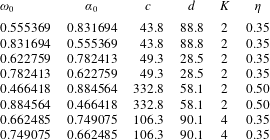
5 Comparison between analytic and numerical solutions
5.1 General attractor modes
In figures 20 and 21 we display the actual eigenfunction for the least-damped eigenmode of attractor
 $\unicode[STIX]{x1D714}_{0}=0.555369$
at
 $E=6\times 10^{-11}$
and the profile of the
 $u_{\unicode[STIX]{x1D711}}$
component across (figure 20
b) and along (figure 21
a) the shear layer as given by (4.38) and the numerical solution. We note the good agreement between the curves: indeed, we expect the relative difference to be of the order of
 $E^{1/12}$
, which is 0.14 at
 $E=6\times 10^{-11}$
. This value is consistent with the magnitude of the difference between the model and the numerical solution as shown in figures 20(b) and 21. A similar result has also been obtained with modes of higher order, and with modes of the attractors listed in table 1.
(a) Meridional distribution of the kinetic energy of the least-damped mode associated with the attractor at
 $\unicode[STIX]{x1D714}_{0}=0.555369$
when
 $E=6\times 10^{-11}$
. The green lines show the actual position of the attractor, while the short and long white lines show the position of transverse and longitudinal profiles displayed in (b) and in figure 21(a). The dashed rectangle delineates the region where the difference between the theoretical and the computed solution has been evaluated. (b) Profile of
 $\text{Re}(u_{\unicode[STIX]{x1D719}})$
and
 $|u_{\unicode[STIX]{x1D719}}|$
for the same mode as in (a) together with the profile of the theoretical prediction (4.38) and the difference between them for 345 segments taken inside the rectangle of panel (a). The solid vertical line visualizes
 $y_{max}$
and the vertical dashed line shows the position of the attractor associated with the mode frequency. The position of the profile is given by the short white line in (a).

(a) Real and imaginary parts of
 $u_{\unicode[STIX]{x1D719}}$
from the numerical and analytical solutions (red and blue lines). The multicolour lines in the middle show the difference between the theoretical prediction (4.38) and the numerical solution at various
 $y$
-positions. (b)
 $u_{\unicode[STIX]{x1D719}}\sqrt{s}/K_{n}$
for the mode shown in figure 20(a) along the associated attractor (green line in figure 20
a);
 $s$
is the distance to axis and
 $K_{n}$
is the amplification factor at the
 $n$
th bounce on the boundary. In black is shown the real part, in red the imaginary part and in green the modulus. The dashed lines in the last interval (long white segment in figure 20
a) show the prediction of (4.38).

(a) Shape of the asymptotic attractor at
 $\unicode[STIX]{x1D714}_{0}=0.7491$
and (b) its symmetrized view. Dashed, dotted and dash-dotted lines are symmetric to the continuous lines of respectively the rotation axis, equator and origin. Arrows indicate the direction chosen along the attractor. (c) The corresponding numerical solution showing a meridional cut of the kinetic energy density (here
 $\unicode[STIX]{x1D702}=0.35$
and
 $E=2\times 10^{-12}$
).

In figure 20(b), we also note that the actual attractor and the asymptotic attractor both stand outside the shear layer. This is because they are at distance
 $O(E^{1/6})$
from
 $y_{max}$
, whereas the shear layer width scales like
 $O(E^{1/4})$
. As a consequence, two shear layers adjacent to the asymptotic attractor do not ‘see each other’ and seem to remain independent, unlike what happens in the analogous two-dimensional problem analysed in Rieutord et al. (Reference Rieutord, Valdettaro and Georgeot2002).
Hence, for a given eigenvalue the foregoing analysis gives a good analytical approximation of the eigenfunction. Our procedure however does not provide the quantization rule of eigenvalues observed numerically.
5.2 Modes with
 $4n$
-reflections on the rotation axis

As we mentioned in the previous section, a special case occurs when the number
 $K$
of reflections on the axis is 0 or a multiple of 4. In these situations, after a full loop along the attractor the factor
 $(-\text{i})^{K}$
due to the reflections on the axis amounts to unity. Therefore the reflections on the axis have overall no effect. Since the governing reduced equation (4.8) is the same as the one we obtained in the two-dimensional toroidal configuration of Rieutord et al. (Reference Rieutord, Valdettaro and Georgeot2002), the same analysis should be valid here as well. We thus expect to find eigenvalues given by the formula obtained in that paper:
 $$\begin{eqnarray}\tilde{\unicode[STIX]{x1D70F}}_{m}=\pm (\tilde{\unicode[STIX]{x1D714}}_{m}-\unicode[STIX]{x1D714}_{0})=-\left(m+{\displaystyle \frac{1}{2}}\right)\sqrt{{\displaystyle \frac{\unicode[STIX]{x1D6FC}_{0}cE}{d}}},\quad m=0,1,2,\ldots ,\end{eqnarray}$$
with eigenfunctions
 $$\begin{eqnarray}p_{m}=U(-m-1/2,z)=\text{e}^{-z^{2}/2}H_{m}(z),\quad z=\text{e}^{-\text{i}\unicode[STIX]{x03C0}/8}(2\unicode[STIX]{x1D6FC}_{0}cd)^{1/4}{\displaystyle \frac{E^{-1/4}y}{B}},\end{eqnarray}$$
where
 $U$
is the parabolic cylinder function and
 $H_{m}=(-1)^{m}\text{e}^{z^{2}}\text{d}^{m}\text{e}^{-z^{2}}/\text{d}z^{m}$
are the Hermite polynomials.
We indeed found such modes. An example is the set of modes associated with the attractor at
 $\unicode[STIX]{x1D714}_{0}=0.74907$
for
 $\unicode[STIX]{x1D702}=0.35$
, shown in figure 22. We report in table 3 the eigenvalues obtained numerically together with the theoretical values given by (5.1). There is a very good agreement between the difference of consecutive eigenvalues and the spacing
 $|\tilde{\unicode[STIX]{x1D70F}}_{2m+2}-\tilde{\unicode[STIX]{x1D70F}}_{2m}|$
given by (5.1). However, the ratio
 $\unicode[STIX]{x1D70F}_{1}/\tilde{\unicode[STIX]{x1D70F}}_{1}$
, between the observed and theoretical damping rates of the fundamental mode is different from 1 and remains close to the value
 ${\sim}1.5$
independently of the Ekman number and of the attractor (see table 3 for the 0.749 attractor). The reason for this discrepancy is very likely due to the fact that we did not consider the corrections induced by the Ekman number to the reflection condition on the axis. Indeed, for the
 $4n$
-attractors that do not cross the polar axis (i.e. with
 $n=0$
), the predicted eigenvalues and eigenfunctions are perfectly verified (see figure 24 and table 4).
(a) Spectrum of attractor
 $0.749$
for
 $E=10^{-10}$
. The red dots are the eigenvalues following the parabolic cylinder solution (5.2). The green eigenvalues follow the multi-scale behaviour (4.38). (b) Profile of the eigenfunction corresponding to the least damped of the red eigenvalues of figure 23(a) at
 $E=3\times 10^{-10}$
.

First eigenvalues for the attractor
 $\unicode[STIX]{x1D714}_{0}=0.7491$
,
 $\unicode[STIX]{x1D702}=0.35$
at two Ekman numbers. The ratio
 $\unicode[STIX]{x1D70F}_{1}/\tilde{\unicode[STIX]{x1D70F}}_{1}\simeq 1.54$
seems to be independent of
 $E$
.
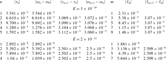
(a) Shape of the attractor at
 $\unicode[STIX]{x1D714}_{0}=0.2958$
,
 $\unicode[STIX]{x1D702}=0.65$
at Ekman number
 $E=10^{-11}$
. (b) The corresponding numerical solution showing a meridional cut of the kinetic energy density divided by the square root of the distance to the polar axis. (c) Profile of the coresponding eigenfunction along the red line of panel (a).

First eigenvalues for the attractor
 $\unicode[STIX]{x1D714}_{0}=0.2958$
,
 $\unicode[STIX]{x1D702}=0.65$
at Ekman number
 $E=10^{-11}$
. Note that
 $\unicode[STIX]{x1D70F}_{1}$
and
 $\tilde{\unicode[STIX]{x1D70F}}_{1}$
are almost equal.

We also remark that even values of
 $m$
do not appear in the numerical solution, but this can be explained by symmetry reasons as follows. The numerical solutions are axisymmetric (see § 2), but they are also symmetric with respect to the equator (see beginning of § 3). On the other hand the asymptotic attractor is symmetric with respect to the equator (see figure 22) but the actual attractor (at
 $\unicode[STIX]{x1D714}\neq \unicode[STIX]{x1D714}_{0}$
) does not have any symmetry. The analytical solution (5.2) for the shear layer along the attractor must therefore be symmetrized in order to fulfil the symmetries imposed to the numerical solution. This is done by adding replicas of the solution along the asymptotic attractor suitably symmetrized with respect to the original one: starting from the attractor denoted with continuous lines in figure 22, we construct three additional attractors: the first is obtained through the axial symmetry (the dashed lines), the second through the equatorial symmetry (the dotted lines) and the third through the combined axial and equatorial symmetry (the dash-dotted lines). The set of these four attractors makes the figure symmetric with respect to both the rotation axis and the equator, as numerically required. For clarity in each panel we label with 1, 1E, 1A and 1EA a given branch of each attractor. The numerical solution is expected to be the same along each of these branches.
The two neighbouring branches marked by 1 and 2E in figure 22 form the shear layer whose profile is shown in figure 23(a). The large-amplitude negative values of
 $y$
belong to the branch 2E while the positive values of
 $y$
correspond to the branch 1. It is readily seen that
 $v_{\unicode[STIX]{x1D719}}(y)$
must be the opposite of
 $v_{\unicode[STIX]{x1D719}}(-y)$
because the reflection on the outer sphere connecting branch 1E to branch 2E produces a change of sign in
 $v_{\unicode[STIX]{x1D719}}$
. The analytical solutions (5.2) with even values of
 $m$
however are even functions of
 $y$
:
 $v_{\unicode[STIX]{x1D719}}(-y)=v_{\unicode[STIX]{x1D719}}(y)$
and are thus forbidden. Those with
 $m$
odd on the other hand are odd functions of
 $y$
and are thus allowed, as we observe numerically. The shape of the least-damped mode (
 $n=1$
) is indeed similar to the predicted one for
 $m=1$
, as we can see in figure 23(a). Here we have considered the 0.749 attractor but the reasoning and the conclusions are valid for all the asymptotic attractors that are equatorially symmetric and have
 $4n$
reflections on axis. We finally remark that if we had solved numerically the equatorially antisymmetric problem, we would have obtained to good precision the two-dimensional eigenmodes corresponding to even
 $m$
values.
(a) Shape of the asymptotic attractor at
 $\unicode[STIX]{x1D714}_{0}=0.6625$
and (b) its symmetrized view. Dashed, dotted and dash-dotted lines correspond are symmetric to the continuous lines with respectively rotation axis, equator and origin. Arrows indicate the direction chosen along the attractor. (c) The corresponding numerical solution showing a meridional cut of the kinetic energy density (here
 $\unicode[STIX]{x1D702}=0.35$
and
 $E=10^{-12}$
).

First eigenvalues for attractor
 $\unicode[STIX]{x1D714}_{0}=0.66249$
,
 $\unicode[STIX]{x1D702}=0.35$
.
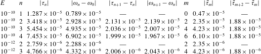
Let us now turn to the case where the asymptotic attractor has
 $4n$
reflections on the axis but no equatorial symmetry, like the attractor plotted in figure 25. One such attractor is obtained by rotating clockwise the attractor of figure 22(a) by
 $\unicode[STIX]{x03C0}/2$
; its frequency is
 $\unicode[STIX]{x1D714}_{0}=0.66249=\sqrt{1-0.74907^{2}}$
. We observed that the eigenvalues associated with this attractor are loosely related to those given by (5.1). The matching between analytics and numerics is much worse than for the previous attractor. The difference also shows up in the eigenfunction: figure 26(a) shows the numerical velocity profile together with the analytic prediction (5.2) for mode
 $n=2$
at
 $E=10^{-12}$
. Despite a very low value of the Ekman number, the two functions still show noticeable differences. This mismatch is due to symmetry requirements of the numerical solution that cannot be satisfied by the analytical solution (5.2). To show this, we first symmetrize the attractor in order to respect the symmetries imposed on the numerical solution (solutions must be axisymmetric and equatorially symmetric). The layout of the attractors after symmetrization is shown in figure 25(b). In this figure the two neighbouring branches marked ‘1’ and ‘2P’ form the shear layer whose profile is shown in figure 26(a). Branch 2P is the continuation of branch 1P, and branch 1P is the mirror symmetric of branch 1. Branch 2P is reached from branch 1P after reflection on the outer boundary and rotation axis. Reflection at the outer boundary produces a change of sign, and crossing of rotation axis produces a
 $-\text{i}$
-factor. We get thus the condition
 $v_{\unicode[STIX]{x1D719}}(-y)=\text{i}v_{\unicode[STIX]{x1D719}}(y)$
. This relation is however not satisfied by any of the functions (5.2). So there cannot be solutions of the type (5.2) as
 $E\rightarrow 0$
. This impossibility likely explains why the
 $n=1$
-mode of the
 $\unicode[STIX]{x1D714}_{0}=0.66249$
-attractor has a frequency that goes out of the range of existence of the attractor when
 $E\leqslant 2\times 10^{-12}$
. The same considerations hold for all the asymptotic attractors that are symmetric with respect to the polar axis with reflections on the axis that are multiples of 4: solutions (5.2) are not expected to exist asymptotically for these modes.
(a) Profile of the eigenfunction corresponding to the least damped of the eigenvalues of the attractor
 $0.66249$
at
 $E=10^{-12}$
. (b) Profile of the eigenfunction corresponding to the least damped of the green eigenvalues of spectrum in figure 23.

We finally note that the shear layer analysis of § 4 is still valid and so we expect to obtain modes described by formula (4.38). Indeed, eigenvalues marked in green in figure 23 correspond to such a case. We show in figure 26(b) the profile of the least damped of these modes and remark that the position of
 $y_{max}$
and
 $y_{attr}$
coincide, which is consistent with (4.42c
) with
 $K=0$
.
6 Conclusions
In this work we continued our investigations of the properties of inertial modes in a spherical shell started in Rieutord & Valdettaro (Reference Rieutord and Valdettaro1997), Rieutord et al. (Reference Rieutord, Georgeot and Valdettaro2001) and Rieutord et al. (Reference Rieutord, Valdettaro and Georgeot2002). The possibility of using more computing power or enhanced precision, allowed us to establish a simple mathematical law (3.2) for the eigenvalues of the modes that are associated with some attractors made of a periodic orbit of characteristics. For these modes, we identified three scales that determine the structure of the shear layers constituting the eigenmodes. These scales are controlled by fractional powers of the Ekman number, namely
 $E^{1/6}$
,
 $E^{1/4}$
and
 $E^{1/3}$
. They singularize the small parameter
 $E^{1/12}$
. This very low power of the Ekman number shows that the true asymptotic regime, such that
 $E^{1/12}\ll 1$
, is not reachable by numerical solutions. It may not even be relevant to the extremely low Ekman numbers met in astrophysics that can hardly go below
 $10^{-18}$
. However, it remains interesting to understand the structure of the solutions when the Ekman number is very small, yet finite.
The present limits of numerical solutions are no longer the available memory, which controls the reachable spatial resolution, but the round-off errors boosted by the ill-conditioned operator. This ill conditioning is related to the singular nature of the inviscid limit of the eigenfunctions. It may be circumvented by using enhanced precision. We therefore place our effort on converting our code to use extended precision (quadruple precision). This choice rapidly reached however the limits of present technology, since computers are all built with double precision arithmetics. Extended arithmetics is therefore obtained through software programming and is thus very slow. This limited our calculations to Ekman numbers above
 $10^{-9}$
. Nevertheless, high-order modes, which are very sensitive to round-off errors, could be properly computed (see also Valdettaro et al.
Reference Valdettaro, Rieutord, Braconnier and Fraysse2007).
The foregoing numerical results obtained on the ‘attractor modes’ guided our analysis of their structure and thanks to the reduced problem (4.8) simplifying the original equation we could determine an analytic formula for the shape of the shear layers. It turns out that an attractor mode is a wave trapped around a characteristic attractor whose typical wavelength is
 $O(E^{1/3})$
but whose envelope has a width
 $O(E^{1/4})$
. This wave packet remains at a distance
 $O(E^{1/6})$
from the asymptotic attractor that has a vanishing Lyapunov exponent. Our analysis does not provide a selection rule for the eigenvalues. It is most likely that the simplifications we made to retrieve the structure of the shear layer are too strong to allow for the determination of the quantization rule of the modes. Our analysis indeed was restricted to the
 $E^{1/3}$
and
 $E^{1/4}$
scales and did not include the
 $E^{1/6}$
one: the condition leading to the quantization of the solution might be more deeply nested in the multiscale dependence of the solutions. The special case where attractors have
 $4n$
reflections on the rotation axis has interestingly extended the applicability of the two-dimensional model solved by Rieutord et al. (Reference Rieutord, Valdettaro and Georgeot2002). However, the predicting power of the two-dimensional model is limited to the frequency spacing of some modes verifying some given symmetries. Here too, some piece seems to be missing for the model to make accurate predictions of eigenvalues and eigenmodes.
Beside attractor modes, we also obtained evidence of the existence of critical latitude modes. These modes are made of detached shear layers emitted by the critical latitude singularity on the inner boundary. They connect the northern and southern critical latitude singularities. Since the path of characteristics from one singularity to that of the other hemisphere is not unique, this set of modes is determined by the set of paths and the transverse wavenumber of the shear layer. The inspection of their damping rates, in the range
 $10^{-9}\lesssim E\lesssim 10^{-7}$
, shows a dependence with the Ekman number close to
 $E^{0.8}$
, meaning a weak dependence of the width of the layers on this number. However, this behaviour does not seem to be asymptotic, since it disappears when
 $E\lesssim 10^{-9}$
for the least-damped mode. More work is needed to fully understand the behaviour of these modes at lower viscosities.
The last category of modes that we identified are a series of modes whose frequency is close to
 $\sin (\unicode[STIX]{x03C0}/4)$
. We recall that when
 $\unicode[STIX]{x1D714}=\sin (\unicode[STIX]{x03C0}/4)$
characteristics follow strictly periodic orbits and thus no small scale is forced by the mapping (Rieutord et al.
Reference Rieutord, Georgeot and Valdettaro2001). The modes of this kind seem to be essentially inertial waves trapped between the two shells. We qualified them as quasi-regular modes because in some range of Ekman numbers they behave as regular modes: their eigenfunction is almost independent of
 $E$
. However, this does not mean that they exist in the inviscid limit. We find that the modes follow quite simple quantization rules, which show that when
 $\unicode[STIX]{x1D714}\rightarrow \sin (\unicode[STIX]{x03C0}/4)$
, the typical wavenumber of the mode tends to infinity and so does the damping rate. This result explains the no-response flow of a fluid in a rotating shell when it is forced periodically at
 $\unicode[STIX]{x1D714}=\sin (\unicode[STIX]{x03C0}/4)$
, as has been observed by Rieutord & Valdettaro (Reference Rieutord and Valdettaro2010). We expect that such a phenomenon occurs for all frequencies leading to neutral periodic orbits of characteristics. With our set-up (aspect ratio
 $\unicode[STIX]{x1D702}=0.35$
), this should also occur when
 $\unicode[STIX]{x1D714}=\sin (\unicode[STIX]{x03C0}/6)$
and
 $\unicode[STIX]{x1D714}=\sin (\unicode[STIX]{x03C0}/3)$
, but inspection of the modes around these frequencies does not show a neat quasi-regular behaviour. Perturbations from the critical latitude singularity appear to be important. For the aspect ratio
 $\unicode[STIX]{x1D702}=0.35$
it seems that only
 $\sin (\unicode[STIX]{x03C0}/4)$
can produce quasi-regular modes, but it turns out that
 $\unicode[STIX]{x1D714}=\sin (\unicode[STIX]{x03C0}/8)$
, for a smaller core (
 $\unicode[STIX]{x1D702}=0.20$
), actually also has quasi-regular modes. Hence, beside the neutral character of periodic orbits, some other character (to be uncovered) is needed to allow quasi-regular modes. Finally, the regularity of the modes, which we characterize by the proportionality of the damping rate to the Ekman number, is lost when the Ekman number is below some value specific to the mode. Thin shear layers appear and introduce a stronger dissipation.
The foregoing solutions, although derived in a highly idealized set-up, show the extreme richness and complexity of the dynamics of rotating fluids. The oscillation spectrum of an incompressible slightly viscous fluid inside a rotating spherical shell appears much more complex than our first studies (Rieutord & Valdettaro Reference Rieutord and Valdettaro1997) let us think. We now clearly see that the eigenvalues cannot be represented by a single formula. Because of the very small powers of the Ekman number (
 $E^{1/12}$
) that seem to control the eigenmodes around attractors, even the astrophysical regime is not in the asymptotic state of vanishingly small quantities. We face here the same difficulty as Sauret & Le Dizès (Reference Sauret and Le Dizès2013) when they studied the libration-induced flows in a spherical shell.
Hence, the asymptotic spectrum at vanishing (but non-zero) Ekman number is most probably a composition of different sets of eigenvalues, which follow their own asymptotic laws. More work is still needed to exhibit the analytical solutions that describe this asymptotic limit like the one obtained by Rieutord et al. (Reference Rieutord, Valdettaro and Georgeot2002) for the two-dimensional problem.
Back to astrophysics and geophysics, which motivate these investigations (since the work of Poincaré Reference Poincaré1885), the various sets of modes and their different asymptotic behaviours will impact the response of the fluid to a global forcing, such as a tidal one. Stars and planets are more complicated systems than our simple spherical shell, but this system has pointed out mechanisms that may persist when stratification or differential rotation (or both) are taken into account (e.g. Dintrans et al. Reference Dintrans, Rieutord and Valdettaro1999; Mirouh et al. Reference Mirouh, Baruteau, Rieutord and Ballot2016).
Acknowledgements
This work was performed using HPC resources from CALMIP (grant 2016-07). We are especially grateful to P. Barbaresco and N. Renon for their assistance in running the very RAM-demanding jobs needed to explore the very low Ekman number space. M.R. acknowledges the support of ISSI (programme on the ‘Seismology of Fast Rotating Stars’, PI J. Ballot) for allowing fruitful discussions on the results of the present work.
Appendix A. Derivation of the reduced equation
We start from the viscous Poincaré equation (4.3) which we rewrite using the
 $(x,y)$
coordinates in the meridian plane instead of
 $(r,z)$
. We note that
 $$\begin{eqnarray}\unicode[STIX]{x0394}^{\prime }={\displaystyle \frac{\unicode[STIX]{x2202}^{2}}{\unicode[STIX]{x2202}x^{2}}}+{\displaystyle \frac{\unicode[STIX]{x2202}^{2}}{\unicode[STIX]{x2202}y^{2}}}+{\displaystyle \frac{1}{4s^{2}}}\end{eqnarray}$$
so that this operator may be reduced to
 $\unicode[STIX]{x2202}^{2}/\unicode[STIX]{x2202}y^{2}$
since we are considering the solution associated with thin shear layers. Thus doing we reduce (4.3) to
 $$\begin{eqnarray}\left(\unicode[STIX]{x1D706}-E{\displaystyle \frac{\unicode[STIX]{x2202}^{2}}{\unicode[STIX]{x2202}y^{2}}}\right)^{2}{\displaystyle \frac{\unicode[STIX]{x2202}^{2}p}{\unicode[STIX]{x2202}y^{2}}}+\unicode[STIX]{x1D714}^{2}{\displaystyle \frac{\unicode[STIX]{x2202}^{2}p}{\unicode[STIX]{x2202}y^{2}}}+2\unicode[STIX]{x1D6FC}\unicode[STIX]{x1D714}{\displaystyle \frac{\unicode[STIX]{x2202}^{2}p}{\unicode[STIX]{x2202}x\unicode[STIX]{x2202}y}}=0.\end{eqnarray}$$
Now focusing on the solutions with the smallest
 $y$
-scales
 $E^{1/3}$
, the term with the largest derivative
 $-E\unicode[STIX]{x2202}^{6}/\unicode[STIX]{x2202}y^{6}$
is negligible. Integrating over
 $y$
and noting that
 $\unicode[STIX]{x1D706}=\unicode[STIX]{x1D70F}+\text{i}\unicode[STIX]{x1D714}$
we get:
 $$\begin{eqnarray}\unicode[STIX]{x1D6FC}{\displaystyle \frac{\unicode[STIX]{x2202}p}{\unicode[STIX]{x2202}x}}={\displaystyle \frac{\unicode[STIX]{x1D706}E}{\unicode[STIX]{x1D714}}}{\displaystyle \frac{\unicode[STIX]{x2202}^{3}p}{\unicode[STIX]{x2202}y^{3}}}+\text{i}\unicode[STIX]{x1D70F}{\displaystyle \frac{\unicode[STIX]{x2202}p}{\unicode[STIX]{x2202}y}}.\end{eqnarray}$$
We can safely replace
 $\unicode[STIX]{x1D6FC}$
with the asymptotic value
 $\unicode[STIX]{x1D6FC}_{0}$
since their difference is
 $O(E^{1/3})$
thus negligible. In this equation the smallest scale,
 $E^{1/3}$
, makes all the terms of the same order (
 $\unicode[STIX]{x1D70F}$
is of order
 $E^{1/3}$
). However, the equation remains valid if, as seen numerically, larger scales and/or contributions to
 $\unicode[STIX]{x1D70F}$
of order
 $E^{1/2}$
are retained.
Appendix B. Reflection on the rotation axis
We show that, for the inviscid case, the reflection on the axis produces a
 $-\text{i}$
factor in the solution. Consider the inviscid axisymmetric solution propagating in the direction of increasing
 $z$
, namely
 $$\begin{eqnarray}p(s,z,t)=p(s)\text{e}^{\text{i}(kz-\unicode[STIX]{x1D714}t)}.\end{eqnarray}$$
The Poincaré equation yields
 $$\begin{eqnarray}\frac{\unicode[STIX]{x2202}^{2}p}{\unicode[STIX]{x2202}s^{2}}+{\displaystyle \frac{1}{s}}\frac{\unicode[STIX]{x2202}p}{\unicode[STIX]{x2202}s}+{\displaystyle \frac{\unicode[STIX]{x1D6FC}^{2}k^{2}}{\unicode[STIX]{x1D714}^{2}}}p=0,\end{eqnarray}$$
which is solved by
 $$\begin{eqnarray}p(s)=A\text{J}_{0}(k_{s}s),\end{eqnarray}$$
where
 $k_{s}=\unicode[STIX]{x1D6FC}k/\unicode[STIX]{x1D714}$
and
 $\text{J}_{0}$
is the zeroth-order Bessel function. Asymptotically, when
 $k_{s}s\gg 1$
, namely far from the rotation axis
 $$\begin{eqnarray}\text{J}_{0}(k_{s}s)\simeq \sqrt{{\displaystyle \frac{2}{\unicode[STIX]{x03C0}k_{s}s}}}\cos \left(k_{s}s-{\displaystyle \frac{\unicode[STIX]{x03C0}}{4}}\right)=\sqrt{{\displaystyle \frac{2}{\unicode[STIX]{x03C0}k_{s}s}}}(\text{e}^{\text{i}k_{s}s-\text{i}\unicode[STIX]{x03C0}/4}+\text{e}^{-\text{i}k_{s}s+\text{i}\unicode[STIX]{x03C0}/4}),\end{eqnarray}$$
which shows that the outward wave
 $$\begin{eqnarray}\text{e}^{\text{i}k_{s}s-\text{i}\unicode[STIX]{x1D714}t-\text{i}\unicode[STIX]{x03C0}/4}\end{eqnarray}$$
is shifted by
 $-\text{i}\unicode[STIX]{x03C0}/2$
compared to the inward wave
 $$\begin{eqnarray}\text{e}^{-\text{i}k_{s}s-\text{i}\unicode[STIX]{x1D714}t+\text{i}\unicode[STIX]{x03C0}/4}\end{eqnarray}$$
if we consider the propagation in a
 $z=\text{Cst}$
plane. We thus conclude that the bounce of the wave on the axis, ingoing and then outgoing, imprints a factor
 $-\text{i}$
on the solution. This behaviour also emerges in the analysis of shear layers produced by a librating disc, which reflect on the axis (e.g. Le Dizès Reference Le Dizès2015).