1. INTRODUCTION
Nowadays, system identification methods are applied in many areas to predict the behaviors of unknown complex systems (Flood & Worley, Reference Flood and Worley1995). Artificial neural networks, genetic algorithms (GAs), fuzzy logic models, particle swarm techniques, and so forth have been recognized to have strong ability in identification, control, and solving unknown systems (Ezziane, Reference Ezziani2002). The more traditional networks necessitate several thousand iterations before they come to the final network. They can be difficult to follow, need profound knowledge of the final network structure, and require a great amount of time to train (Gilbar, Reference Gilbar and Pandya2002).
Most of the programs available for artificial neural networks do not develop the network by assigning weights. Rather, they train the networks to give the output they seek for a particular input and then record the weights (Bishop, Reference Bishop1995). Several methods exist that modify the basic neural network structures. They were designed to be very general and hence do not capture the trend very well. An example of such a method could be Multilayer Perceptron (Jia, Reference Jia1998; Tourenq et al., Reference Tourenq, Brosse, Guegan and Lek1999; Kim & Adalı 2000; Cai et al., 2002). These methods have a tendency to avoid overfitting, and thus they do not produce exact results. Further, some algorithms produce very large networks to bring about accurate results that are proved ineffective and difficult to carry out using hardware as a result of their complexity.
The algorithm of group method of data handling (GMDH) method has been applied strongly in identification and solving complex nonlinear systems. The GMDH method is a heuristic self-organization modeling method that was first introduced by Ivakhnenko (Reference Ivakhnenko1995) as a rival to the method of stochastic approximation. In other ways, the GMDH technique is defined as a method to construct a higher polynomial model that is extended to constructing a higher and optimal logical model. This method produces a structure of partial descriptions, which is described by quadratic regression polynomials (i.e., can allow more than one input), and then its output is evaluated for fitness using the criterion error. The number of created neurons in each layer and also the number of layers during the process is self-organized in GMDH models. In this self-organizing algorithm, a model is generated from data in the form of networks of active neurons in a repetitive generation of competing models of growing complexity and corresponding validation (Buryan et al., Reference Buryan, Onwubolu and Lemke2008). Readers who wish to gain a more insightful understanding of fundamental concepts of GMDH are recommended to read the following books, which are among the best in the field: Farlow (Reference Farlow1984), Madala and Ivakhnenko (Reference Madala and Ivakhnenko1998), and Müller and Lemke (Reference Müller and Lemke1999).
Although GMDH offers a systematic procedure of system modeling and prediction, it also suffers from a number of shortcomings. One hurdle could be the fact that the network created using this algorithm will have neurons calculated using a quadratic polynomial. This helps to find out the exact relationship between neurons in the preceding layer; even for the most complicated networks, this will be easily understandable. In addition, the algorithm should create a balance between complexity and accuracy. With the advent of GMDH, there have been variants developed from different angles to evaluate coefficients to lessen the problems resulting from the standard GMDH algorithm (Iba et al., Reference Iba, Garis, Sato and Kinnear1994; Robinson, Reference Robinson1998; Hiassat et al., Reference Hiassat, Abbod, Mort and Hamparsum2003; Park et al., Reference Park, Park, Kim and Oh2004; Oh et al., Reference Oh, Park, Pedrycz, Ahn, Sunderam, van Albada, Sloot and Dongarra2005).
Among the approximation methodologies to improve the accuracy of estimation in GMDH algorithms, a statistical-based method, called the least squares method, has been employed in calculating the coefficients. In many cases, simulation models encounter issues with a common problem known as an inverse problem in a mathematical model. There are some algorithms to solve this kind of difficult problem.
Levenberg–Marquardt (LM) algorithms have recently turned out to be a valuable means for ensuring fast convergence to a solution of the nonlinear system and singularity problem. Gradient-based techniques such as the LM have a high dependence on the initial guess, which is generally not known to the user. Thus, the user has to undertake many trials with various initial guesses to arrive at the global optimum. However, the initial guess is crucial to the success of the heuristic search for an optimal model. The benefits of the LM may lessen if the initial guess is not adequately close to the actual value.
To avoid being trapped in a local minimum, a detailed investigation on this front has led to the innovation of a new idea in order to ensure the global convergence of the LM method. We minimize the target function by generating the initial guess using a singular value decomposition (SVD) method, and then we select only those values of the fitting parameters that give the lowest value of the target function. The most popular technique for the SVD method of computing was introduced by Golub and Reincsh in 1970. The SVD method is a very useful method in solving most linear least squares problems, such as matrix inversion, overdetermined, and underdetermined systems of linear equations where some singularities may exist in the normal equations (Press et al., Reference Press, Flannery, Teukolsky and Vetterling1986; Onwubolu, Reference Onwubolu2008).
The modified LM algorithm is adjusted for decreasing the computational time in the classic LM algorithm. In addition, because the LM algorithm requires a large number of function evaluations to converge to the global optimum, it may be advisable to terminate it when the improvement in the target function is small and the design space has been explored significantly. Implementations of the modified LM algorithm have a good convergence rate and need less iteration to convergence compared to the classical LM algorithm. Moreover, this technique yields improved computational efficiency when the LM method is used as the optimization technique for GMDH.
2. REVIEWED LITERATURE
Over the past 40 years, the GMDH-type algorithm has been a subject that attracted scientists' attention (Ivakhnenko, Reference Ivakhnenko1968, Reference Ivakhnenko1995; Shankar, Reference Shankar1972; Farlow, Reference Farlow1984; Lemke, Reference Lemke1995; Muller et al., Reference Muller, Barton and Benignus1984; Müller, Reference Muller, Barton and Benignus1996; Nikolaev & Iba, Reference Nikolaev and Iba2003; Thakkar, Reference Thakkar2011). In order to improve the accuracy of the prediction, the LM method is adopted in this paper. Still, there is a lot of literature on improving the initial guess factor of the LM method (Xiang et al., Reference Xiang, Cheng, Schlindwein and Jones2003; Walker et al., Reference Walker, Varadan and Fushman2004; Sedighi et al., Reference Sedighi, Khandaei and Shokrollahi2010; Parente et al., Reference Parente, Makarewicz and Bishop2011). Xiang et al. developed a direct inversion algorithm for the “optimal estimation”; the new algorithm differs from the existing one in that there is no need for an initial guess for initialization and the estimated parameters are direct solutions of a set of equations (Xiang et al., Reference Xiang, Cheng, Schlindwein and Jones2003).
Walker and colleagues presented a “novel computer program” named ROTDIF in 2004 with the aim of “computational efficiency and accuracy.” They instrumented a “six-dimensional optimization search” using an efficient LM algorithm combined with “Monte Carlo generation” of initial guesses. The improvement of this method is its high sensitivity, robustness, and significant time saving nature compared to all previous approaches in this area of study (Walker et al., Reference Walker, Varadan and Fushman2004). In addition, Sedighi et al. (Reference Sedighi, Khandaei and Shokrollahi2010) worked on an “inverse problem of optimization” approach based on LM to identify the parameters of two different material constitutive models. They showed that the parameters have relatively very low dependency on the initial guess in numerical algorithm. Finally, Parente et al. (Reference Parente, Makarewicz and Bishop2011) developed a new Gaussian modeling based on “automatic initial parameter estimation” and examined its performance with the existing technique in modeling of the absorption band. In their study, the “nonlinear curve fitting techniques” were examined by the LM algorithm and the total inversion algorithm in terms of “accuracy” and “sensitivity analysis of the fitting results to small variations of the initial parameter estimates.”
3. GMDH-TYPE NEURAL NETWORK USING MODIFIED LM
3.1. The basic GMDH algorithm
The GMDH algorithm can be represented as a set of neurons in each layer, connected through a quadratic polynomial that generates new neurons in the next layer. Ivakhnenko (Reference Ivakhnenko1995) employed the Kolmorovo–Gaborov sentence, which proves that every function y(n) = f(x) can be represented by an infinite Volterra–Kolmogorov–Gabor polynomial of the form
 $$y_n=a_0+\sum\limits_{i=1}^M {a_i } x_i+\sum\limits_{i=1}^M {\sum\limits_{\,j=1}^M {a_{ij} } } x_i x_j+\sum\limits_{i=1}^M {\sum\limits_{\,j=1}^M {\sum\limits_{k=1}^M {a_{ijk} } } } x_i x_j x_k \cdots \comma \;$$
where X(x 1, x 2, … , x M) is the vector of input variables, A(a 1, a 2, … , a M) is the vector of coefficients or weights, and M is the number of input variables.
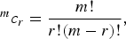
With the increase of M, this equation can lead to very difficult calculations due to the high order of the resulting polynomial. The Volterra–Kolmogorov–Gabor series is estimated by second-order polynomials using only two new variables of neurons (Müller et al., Reference Müller, Lemk and Ivakhnenko1994; Madala et al., Reference Madala and Ivakhnenko1998; Godfrey et al., Reference Godfrey, Petr and Frank2007). The number of combinations generated before learning each layer is
 $$^m c_r=\displaystyle{{m!} \over {r!\lpar m - r\rpar !}}\comma \; $$
where m is the number of input variables and r is the number of points for each node. Furthermore, all combinations of two independent variables are generated in this form:
 $$G\lpar x_i\comma \; x_j \rpar =a_0+a_1 x_i+a_2 x_j+a_3 x_i x_j+a_4 x_i^2+a_5 x_j^2. $$
In Equation (3), G(x i, x j), x i, and x j indicate the outputs of multilayered composition and inputs variables, respectively. The combinations of two independent variables are illustrated in the schematic diagram in Figure 1.
(Color online) Schematic diagram of the combinations of two variables.

Consequently, in this problem, there will be six unknown coefficients for each neuron. The following equations can be obtained:
 $$Xa=Y\comma \; $$
and
 $$a=\lsqb a_0\comma \; a_1\comma \; a_2\comma \; a_3\comma \; a_4\comma \; a_5 \rsqb \comma \; $$
where a is the vector of unknown coefficients of the quadric polynomial in Equation (3).
Accurate coefficients improve the performance of self-organizing GMDH-type algorithms. The nonlinear least square method is an important statistical-based method to calculate the coefficients for any neuron design procedure in the training data. Other approaches applied include the gradient descent and Gauss–Newton methods (Ivakhnenko, Reference Ivakhnenko1995; Hiassat et al., Reference Hiassat, Abbod, Mort and Hamparsum2003; Nariman et al., Reference Nariman-Zadeh, Darvizeh, Jamali and Moeini2009). However, singularity is the most important mathematical problem for solving the inverse of matrix in mathematical models. To alleviate the inverse problem in the least square method, many researchers consider developing new algorithms. Papers (Jiang et al., Reference Jiang, Xia and Shou2006; Naveen et al., Reference Naveen, Jayaraman, Ramanath and Chaudhuri2010) have proposed a new algorithm that is referred to as a modified LM algorithm. Their results show some improvements in the LM algorithm, although they do not achieve any significant advantage when the initial guess is nt sufficiently close to the actual value. We present a procedure to produce an appropriate initial guess by using the SVD technique. Then, the best set of these newly generated neurons are selected and used for the next layer according to a selection criterion.
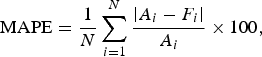
The mean absolute percentage error (MAPE) expresses the forecasting errors from different measurement units into percentage errors on actual observations. Therefore, the MAPE is probably the most widely used method of forecasting accuracy measurement of this kind (Goodwin & Lawton, Reference Goodwin and Lawton1999). It is used to select the polynomials for proceeding to the next layer, and it expresses the accuracy as a percentage that is defined by the following formula:
 $${\rm MAPE}=\displaystyle{1 \over N}\sum\limits_{i=1}^N {{\displaystyle{\left\vert {A_i - F_i } \right\vert \over A_i }} \times 100}\comma \; $$
where N is the total of number of data, A i is the measurement value, and F i is the prediction value corresponding to the system output. The model of the data can be computed by tracing back the path of the polynomials that corresponds to the lowest MAPE in each layer (Müller et al., Reference Müller, Lemk and Ivakhnenko1994). This procedure is repeated for each neuron of the next hidden layer until only one neuron remained in the last layer. It may be noted that there are other criteria as well for selecting neurons in each layer as input variables for the next layer (Kondo & Pandya, Reference Kondo, Pandya and Negoita2004).
3.2. The LM algorithm
The LM algorithm is a well-known mathematical method for solving data matching problems in nonlinear systems. The LM algorithm is a hybrid algorithm, which is self-adaptive (Dan et al., Reference Dan, Yamashita and Fukushima2002; Kanzow et al., Reference Kanzow, Yamashita and Fukushima2004), and one of the least square curve fitting methods.
In fitting a function  $\hat y\, \lpar x\semicolon \; p\rpar $ of an independent variable x and a vector of n parameters p to a set of data points (x i, y i), it is convenient to minimize the sum of the weighted squares of the errors. This scalar-valued measure is called the chi-squared error criterion. The weights included in the GMDH are defined as the vector w, and the objective function is given by
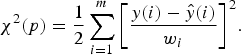 $${\rm {\chi}} ^2 \lpar {p}\rpar =\displaystyle{1 \over 2}\sum\limits_{i=1}^m {\left[{\displaystyle{{y\lpar i\rpar - \hat y\lpar i\rpar } \over {w_i }}} \right]} ^2.$$
The main objective of the data matching is to minimize the objective function. The perfect value is zero, where x = (x 1, x 2, … , x n) and F(x):R n → R m is a nonlinear continuously differentiable function. The solution set of Equation (7) is nonempty and is denoted by
 $$x:=\left\{{x \in \left. {R^n } \right\vert F\lpar x\rpar =0} \right\}\comma \; $$
The LM method updates the relationship by the following equation:
 $$[{J\lpar x_k \rpar ^T J\lpar x_k \rpar +{\rm \mu} I} ]\lpar \Delta x\rpar ^k=- J\lpar x_k \rpar ^T f\lpar x\rpar \comma \; $$
where µ is the damping parameter used to overcome singularity difficulties of J(x k), J is the Jacobian matrix, and J(x k) = F ′(x k). The parameter µ will be set to a large value in the beginning of iterations, and in each iteration, if F(x k + Δx k) < F(x k−1 + Δx k−1), decrease µ by a specific amount to speed up the convergence. Moreover, LM benefits may also be reduced if the initial guess is not adequately close to the actual value. In this case, it will have slow convergence or a local converge, which gives an undesirable match (Dan et al., Reference Dan, Yamashita and Fukushima2002; Fliege et al., Reference Fliege, Drummond and Svaiter2009).
Optimal parameters have recently been chosen by some researchers (Yamashita & Fukushima, Reference Yamashita and Fukushima2000; Fan & Yuan, Reference Fan and Yuan2001). Their results show some improvements in the LM algorithm, although they do not achieve any significant advantage when solutions are not sufficiently close to the actual value. In this research work, we use the outcome of the SVD method as an initial guess for the input of the LM method. This technique yields improved computational efficiency when the LM method is used as the optimization technique for GMDH.
3.3. Framework of the design procedure of the GA-based enhanced GMDH
Overall, the framework of the design procedure of the proposed GA-based GMDH comes as a sequence of the following steps:
Step 1. Determine the initial information for constructing the GMDH structure. The structure can be determined in the following manner:
a. the maximum number of layers and the number of nodes per layer;
b. the maximum number of input variables arriving at each node and the polynomial types used; and
c. the GA parameters: these parameters are population size, crossover rate, mutation rate, and the stopping criterion. In this study, the maximum number of generations is used as the stopping criterion.
Step 2. Form a training and validation data: the input data set is divided into two parts: that is, a training data set and a testing data set. The size of the training data set is two times more than the size of the testing data set.
Step 3. Generate an initial population: the polynomial type of each node, the number of inputs of each node, and the input variables chosen to each node are encoded into a chromosome, and these chromosomes are all randomly initialized.
Step 4. Estimate the coefficient parameters of each node: the vector of coefficient parameters is derived by minimizing the locally weighted mean squared error as is given in the previous section. This procedure is implemented repeatedly for all nodes.
Step 5. Check the stopping criterion: the modeling can be terminated when the stopping criterion is reached. If the stopping criterion is not satisfied, the model has to be expanded. Steps 3 and 4 can be repeated until the stopping criterion is satisfied.
Step 6. After the evolution process, the chromosome, which has the best performance in the last generation, is selected as the final structure of the network. The output of the selected network is the predicted value of the current query point. Then, Steps 2 to 6 can be repeated until the future values of different query points are all acquired.
In order to illustrate the benefits of our algorithm, a comparison between the basic GMDH algorithm and the GMDH-LM algorithm is made. It has been applied in an inventory control system in a Malaysian manufacturing company.
4. EXPERIMENTAL RESULTS AND DISCUSSION
The use of modeling and simulation technologies is very popular in modeling complex inventory systems. One of the most important conditions that must be met in just-in-time systems is inventory control, and a Kanban system is a decentralized system in inventory control that harmoniously controls the production of the necessary products in the essential quantities in the required time.
One of the most important conditions that must be met in Kanban systems is the aid of accurate prediction in the average time in system of products on the final assembly line. The imbalance of time in inventory control influences the process activities and the amount of order from subcontractors. In this study, we have proposed a GMDH architecture for predicting the average time in Kanban systems, which is presented for the first time in this research.
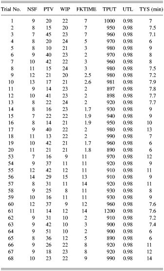
In this step, the proposed network generates a structure of the model by the selected data. All 68 trials were collected from the industry to do preliminary validation of the proposed method. The outputs and measures that were obtained for the 68 trial inputs are shown in Table 1. The input parameters are the number of stages on the feeder line, level of processing time variability, average time in system of the products being assembled at the workstation on the final assembly line, average work in process on the feeder line, average waiting times of the production ordering and withdrawal Kanbans on the feeder line, throughput at the workstation on the final assembly line during a shift, and average utilization of all the stages on the feeder line. This data set constituted six inputs and one output. The targets for average time in Kanban system are given in the last columns of Table 1.
(Color online) The performance index on training and testing data for two layers.
Values for operational factors associated with the Kanban
Note: NSF, number of stages on the feeder line; PTV, processing time variability; WIP, average work in process on the feeder line; FKTIME, average waiting times of the production ordering and withdrawal Kanbans on the feeder line; TPUT, throughput at the workstation on the final assembly line during a shift; UTL, average utilization of all of the stages on the feeder line; TYS, average time in the system of the products being assembled at the workstation on the final assembly line.
The data have been divided into two sets: training and testing sets. The training set consists of 43 out of the 68 input–output data pairs, and the testing set consists of 43 input–output data samples. We use SVD method to produce an appropriate initial guess in the LM method and generate the intermediate variables. The outputs of these values are selected for entry to the next layer, and only elements whose performance is acceptable survive to form the next layer. This process is continued as long as each layer subsequently produced a better result than the previous layer. When the error of the test data prediction is not better than the last layer, the process is stopped and the iterative computation is terminated.
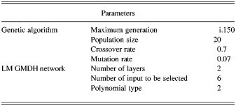
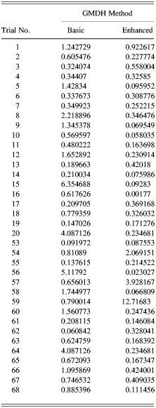
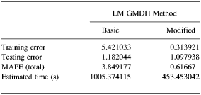
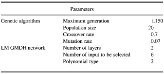
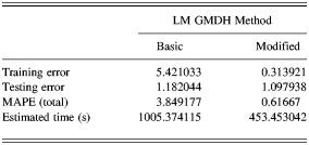
Table 2 shows the GA's parameters and the initial information of the LM GMDH network, which will be optimized to get the best structure of the network for the current query point. Table 3 shows the comparison of predicted error values for average time on the final assembly line. It can be seen that the errors reduce from the basic GMDH to the LM GMDH model, and Table 4 shows the comparison of errors, MAPE, and estimated time in different LM GMDH neural networks methods. These results show that our proposed method outperforms the basic LM GMDH method. The behavior of the basic GMDH and the LM GMDH neural network models are depicted in Figure 2. It shows that the accuracy of results modeled by this enhanced GMDH is considerably high with reasonable reduction in processing time. There is an important fact in optimal design between objective functions; it is required that all conflicting objectives, training error, testing error, and number of hidden layers (representing the complexity of the models) be minimized simultaneously.
Design parameters of the proposed method
Note: LM, Levenberg–Marquardt; GMDH, group method of data handling.
A comparison of the MAPE at two layers for basic and enhanced GMDH methods
Note: MAPE, mean absolute percentage error; GMDH, group method of data handling.
A comparison of MAPE and estimated time
Note: MAPE, mean absolute percentage error; LM, Levenberg–Marquardt; GMDH, group method of data handling.
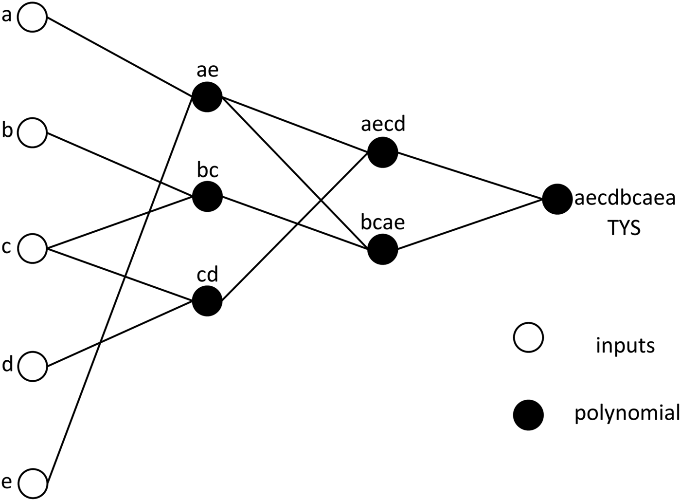
The excellent behavior of such GMDH-type networks in modeling and prediction in conjunction with improved the LM approach is also depicted in Figure 3. As could be observed, the predicted values closely follow the experimental results, except for trial numbers 49, 57, and 59, where there are some noticeable deviations. Figure 4 shows the LM GMDH prediction and absolute difference error. Figure 5 shows the graphical representation of the network connections for LM GMDH; this figure is very useful for understanding how the winning nodes are connected from layer to layer until the network realizes a final solution at the output layer. The structure of such evolved two-hidden layer GMDH-type neural networks is also shown in Figure 5, and the following best model was generated:
(Color online) The actual and predicted plots by the Levenberg–Marquardt group method of data handling. TYS, average time in the system of the products being assembled at the workstation on the final assembly line.
(Color online) The Levenberg–Marquardt group method of data handling prediction and absolute difference errors.
Graphical representation of Levenberg–Marquardt group method of data handling network connections structure for Kanban system.
$$\eqalignno{ z_1 & =- 32.9652+0.153768\quad a+0.076551\quad e - 0.12999 \cr& \quad \;\,a^2 - 4.6E - 05\quad e^2+0.002662\quad a e \cr z_2 &=12.43097+0.120575\quad b - 0.123869\quad c - 0.0191\cr & \quad \;\,b^2 +- 0.06303\quad c^2+0.054208\quad cb \cr z_3 & =- 0.36839+0.511909\quad c - 0.835033\cr & \quad \;\,d -0.00839\quad c^2 +- 0.0292\quad d^2+0.000613\quad cd \cr f_1& =409.0847 - 43.2289\quad z_1 - 36.9531\quad z_3+1.268331\cr & \quad \;\,z_1 ^2 +0.908063\quad z_3 ^2+1.789357\quad z_1 z_3 \cr f_2&=58.70075+1.254165\quad z_1 - 11.8796\quad z_2 - 0.13131\cr & \quad \;\,z_1 ^2+0.518262\quad z_2 ^2+0.166494\quad z_1 z_2 \cr {\rm TYS} & =67.4449 - 3.23016\quad f_1 - 8.29554\quad f_2+0.063436\cr & \quad \;\,f_1 ^2 +0.248207\quad f_2 ^2+0.220129\quad f_1 f_2 }$$where TYS is the average time in system of the products being assembled at the workstation on the final assembly line.
5. CONCLUSION
We introduced an enhanced GMDH algorithm that enables us to predict the nonlinear phenomenon. We presented a procedure to produce a model, and then we improved the predictive model by the modified LM method. This technique yielded improved computational efficiency. This approach is more flexible and generalized than the other enhanced GMDH models. Note that some disadvantages of basic GMDH algorithms can be solved by effective improvement efforts. In order to demonstrate the prediction ability in the proposed GMDH neural networks, an optimized methodology was presented for finding the optimal solutions for the experimental data in Kanban systems. Moreover, the testing results showed that the lag-adjusted model was very accurate and in some cases almost as exact as the measured time values in the Kanban system.
Maryam Pournasir is currently a PhD student in computer science at the University of Multimedia Malaysia and graduated from the University of Guilan, Rasht, Iran.
Md. Jahangir Alam is a Research Assistant in the Faculty of Science and Engineering at Deakin University, Australia. He was formerly an Assistant Professor in the Department of Computer Engineering at Jahangirnagar University and a Lecturer in the Faculty of Computing and Informatics at Multimedia University. Dr. Alam received his BS and MS from the Department of Physics at Jahangirnagar University in 1989 and 1991, respectively, and his PhD from the Department of Physical Electronics & Informatics at Osaka City University in 2004. His research interests include computer vision, pattern recognition, image processing, human–computer interaction, telemedicine, and data modeling.
Govindan Marthandan is an Associate Professor and the Deputy Dean of the Graduate School of Management at Multimedia University Malaysia. He received his BEng, MEng, and PhD from the University of Madras India and an MBA in operations management from IGNOU, India. His areas of interest include information system development, information system evaluation, ICT applications, Web data mining, E-commerce, and supply chain management. Dr. Marthandan is currently supervising many PhD, DBA, and MBA postgraduates. He has vast experience working with information technology in industry and government and academic institutions.