1 Introduction
Thin elastic membranes enclosing liquids, which have come to be called capsules, are central to many applications. They are manufactured for purposes such as inkjet printing (Leelajariyakul, Noguchi & Kiatkamjornwong Reference Leelajariyakul, Noguchi and Kiatkamjornwong2008), use in cosmetics (Miyazawa et al.
Reference Miyazawa, Yajima, Kaneda and Yanaki2000; Martins et al.
Reference Martins, Barreiro, Coelho and Rodrigues2014), releasing aromas and flavours (Gibbs et al.
Reference Gibbs, Kermasha, Alli and Mulligan1999; Pop Reference Pop2011) and absorbing
 $\text{CO}_{2}$
in gas plumes (Vericella et al.
Reference Vericella, Baker, Stolaroff, Duoss, Hardin, Lewicki, Glogowski, Floyd, Valdez, Smith, Satcher, Bourcier, Spadaccini, Lewis and Aines2015). Similarly, they are attractive for biomedical applications, including drug delivery (Lim Reference Lim1984; Dey, Majumdar & Rao Reference Dey, Majumdar and Rao2008; Paret et al.
Reference Paret, Trachsel, Berthier and Herrmann2015), contrast-enhanced ultrasound imaging (Furlow Reference Furlow2009) and the development of artificial blood and organs (Kuhtreiber, Lanza & Chick Reference Kuhtreiber, Lanza and Chick1998; Chang Reference Chang2010). The collective flow of such suspensions depends upon the dynamics of the capsules, which has motivated extensive studies (Barthès-Biesel Reference Barthès-Biesel2016). The stability of the capsule motion when subject to shear flow is expected to be important for their behaviour, either in isolation or in dense suspensions. If the capsule motion is steady or periodic for particular flow conditions, we anticipate less overall flow resistance than if it is fundamentally unstable. Unsteady capsule motion can also be expected to cause additional stress on the capsule membranes themselves, which are often fragile (Goosen et al.
Reference Goosen, O’Shea, Gharapetian, Chou and Sun1985; Gåserød, Sannes & Skjåk-Bræk Reference Gåserød, Sannes and Skjåk-Bræk1999). Studies of capsule stability have been based on observations, especially in simulation models. We develop a complementary direct stability analysis of the coupled capsule–shear-flow system. Similarly to the primarily empirical studies that guide us, our analysis is based on numerical methods. However, these methods are used here to construct a linearized system for analysis, which is advantageous in that it predicts the linear behaviour of the complete basis of membrane perturbations included in the numerical discretization, not necessarily just those directly observed in flow simulations.
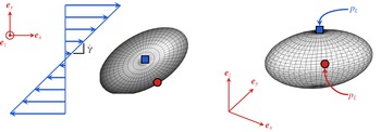
The capsule–homogeneous-shear-flow configuration;
 $p_{\unicode[STIX]{x1D709}}$
and
 $p_{\unicode[STIX]{x1D701}}$
are points used to define deformation and motion in § 2.

We consider both spherical and ellipsoidal capsules in homogeneous shear flow, as shown schematically in figure 1. This configuration can produce rich and varied capsule kinematics, depending upon the capsule shape and flow strength (Dupont, Salsac & Barthès-Biesel Reference Dupont, Salsac and Barthès-Biesel2013). Simulation-based studies have both considered the viscous Stokes-flow limit (Dupont et al.
Reference Dupont, Salsac and Barthès-Biesel2013, Reference Dupont, Delahaye, Barthès-Biesel and Salsac2016) and included finite inertia (Cordasco & Bagchi Reference Cordasco and Bagchi2013; Wang et al.
Reference Wang, Sui, Spelt and Wang2013); here, we only consider the viscous limit. For prolate capsules, weak flow and long times, capsules have been observed to reach an apparently steady rolling or tank-treading motion, for which the membrane rotates in the shear plane about a deformed capsule shape (Dupont et al.
Reference Dupont, Salsac and Barthès-Biesel2013). Such a configuration is visualized in figure 1, with
 $\boldsymbol{e}_{x}$
–
 $\boldsymbol{e}_{y}$
spanning the nominal shear plane. For stronger shear, in addition to rotation, the capsule also precesses around the base-flow vorticity axis (
 $\boldsymbol{e}_{z}$
), and for still stronger shear, a so-called swinging motion is observed, where a time-periodic deformation cycle appears in addition to the tank-treading motion (Dupont et al.
Reference Dupont, Salsac and Barthès-Biesel2013; Wang et al.
Reference Wang, Sui, Spelt and Wang2013). Oblate capsules have been observed to undergo similar motion at long times (Cordasco & Bagchi Reference Cordasco and Bagchi2013; Wang et al.
Reference Wang, Sui, Spelt and Wang2013; Dupont et al.
Reference Dupont, Delahaye, Barthès-Biesel and Salsac2016). For weak flows, oblate capsules take on a swinging motion, and can wobble with increasing shear rate. In this case, the capsule orientation oscillates about an axis not aligned with the shear-flow vorticity. For sufficiently strong shear rates, the capsule rolls, its deformed membrane rotating about the
 $\boldsymbol{e}_{z}$
axis (Dupont et al.
Reference Dupont, Delahaye, Barthès-Biesel and Salsac2016).
Simulations suggest that the long-time capsule orientation and cyclic motion are independent of the initial capsule orientation, as quantified by the angle of the longest principal axes of a fitted ellipsoid with respect to the shear plane (Dupont et al. Reference Dupont, Salsac and Barthès-Biesel2013, Reference Dupont, Delahaye, Barthès-Biesel and Salsac2016). However, there is some ambiguity in reported results (Cordasco & Bagchi Reference Cordasco and Bagchi2013), which has been hypothesized to result from insufficient observation times (Dupont et al. Reference Dupont, Delahaye, Barthès-Biesel and Salsac2016). It is a challenge with finite-time simulations to determine unambiguously that longer times do not yield qualitatively different conclusions. Such observations also do not directly classify the stability, and risk missing kinematic behaviour that might be sensitive to initial perturbations. Particular deformations are known to be unstable in other flows, such as a slender capsule subjected to strong extensional flow (Zhao & Shaqfeh Reference Zhao and Shaqfeh2013) and capsule trains flowing within channels (Bryngelson & Freund Reference Bryngelson and Freund2016) and tubes (Bryngelson & Freund Reference Bryngelson and Freund2018). Our goal is to classify the stability of capsules in shear flow based on analysis of the corresponding linear system. We develop a linear stability analysis that includes a complete basis (for the selected spatial resolution) of capsule membrane perturbations, as represented with spherical harmonic functions. This is used to determine the rate at which perturbations grow or decay.
We consider perturbations to the fixed-point configurations deduced in previous simulation studies (Dupont et al. Reference Dupont, Delahaye, Barthès-Biesel and Salsac2016) and analyse the stability of the periodic rotation with Floquet methods. Similar methods have been used to classify the stability of flow in periodically forced lid-driven cavities (Cazemier, Verstappen & Veldman Reference Cazemier, Verstappen and Veldman1998; Blackburn & Lopez Reference Blackburn and Lopez2003), periodic vortex streets shed by rings (Sheard, Thompson & Hourigan Reference Sheard, Thompson and Hourigan2003, Reference Sheard, Thompson and Hourigan2004) and square and circular cylinders (Barkley & Henderson Reference Barkley and Henderson1996; Gioria et al. Reference Gioria, Jabardo, Carmo and Meneghini2009; Sheard, Fitzgerald & Ryan Reference Sheard, Fitzgerald and Ryan2009), pulsatile channel (Von Kerczek Reference Von Kerczek1982; Pier & Schmid Reference Pier and Schmid2017) and pipe flows (Blennerhassett & Bassom Reference Blennerhassett and Bassom2007; Thomas, Bassom & Blennerhassett Reference Thomas, Bassom and Blennerhassett2012), and Stokes layers adjacent to oscillating boundaries (Blennerhassett & Bassom Reference Blennerhassett and Bassom2002; Davies et al. Reference Davies, Thomas, Bassom and Blennerhassett2015; Thomas et al. Reference Thomas, Blennerhassett, Bassom and Davies2015). These studies generally rely to some degree upon numerical methods, as does ours. Few Floquet studies include fluid–structure interaction; the present analysis is perhaps most closely related to the Floquet analysis of axisymmetric rigid particles in shear flow with weak inertia (Einarsson, Angilella & Mehlig Reference Einarsson, Angilella and Mehlig2014), although in that case the rigid-particle dynamics allows for a tractable analytic linearization of the governing equations about the periodic particle motion. The deformable membrane introduced here presents additional complexity that seems to preclude direct extension of that formulation.
The details of the specific configurations we consider are introduced in § 2. The numerical methods used for constructing the periodic base flow, the stability analysis and the corresponding direct numerical simulations (DNS) are summarized in § 3. We verify that our simulations reproduce particular results of previous studies in § 4; these also provide the time-periodic base flows for our subsequent Floquet analysis. The stability analysis is developed in § 5, with results presented in § 6 for a range of flow strengths.
2 Capsule–flow system
The initial capsule shape
 $\boldsymbol{x}=\{x,y,z\}$
in figure 1 is a spheroid with
 $$\begin{eqnarray}\frac{x^{2}+y^{2}}{b^{2}}+\frac{z^{2}}{a^{2}}=1,\end{eqnarray}$$
where
 $a/b$
is the aspect ratio and
 $r_{o}=(b^{2}a)^{1/3}$
is the radius of a sphere of the same volume. The capsule perturbs a homogeneous shear flow,
 $$\begin{eqnarray}\boldsymbol{u}^{\infty }(\boldsymbol{x})=\dot{\unicode[STIX]{x1D6FE}}y\boldsymbol{e}_{x},\end{eqnarray}$$
where
 $\dot{\unicode[STIX]{x1D6FE}}$
is the shear rate. Following Dupont et al. (Reference Dupont, Delahaye, Barthès-Biesel and Salsac2016), we define
 $\unicode[STIX]{x1D701}(t)$
as the instantaneous angle between the
 $\boldsymbol{e}_{z}$
axis and the shortest capsule principal axis. Similarly,
 $\unicode[STIX]{x1D709}(t)$
is the angle between the
 $\boldsymbol{e}_{z}$
axis and a segment extending from the capsule centre to the point that was initially on the shortest principal axis at time
 $t=0$
. The corresponding points on the capsule are
 $p_{\unicode[STIX]{x1D701}}$
and
 $p_{\unicode[STIX]{x1D709}}$
, as labelled in figure 1. Both the interior and the exterior fluid are Newtonian and incompressible with the same viscosity
 $\unicode[STIX]{x1D707}$
.
The capsule membrane elastic resistance is described using the Skalak constitutive model (Skalak et al. Reference Skalak, Tozeren, Zarda and Chien1973) with strain energy
 $$\begin{eqnarray}W=\frac{E_{s}}{8}(I_{1}^{2}+2I_{1}-2I_{2})+\frac{E_{d}}{8}I_{2}^{2},\end{eqnarray}$$
where
 $E_{s}$
is the shear modulus,
 $E_{d}=CE_{s}$
is the dilatation modulus (where
 $C$
sets its relative strength) and
 $I_{1,2}$
are the usual strain invariants. Bending is resisted through a linear isotropic model (Zhao et al.
Reference Zhao, Isfahani, Olson and Freund2010) with bending moment
 $$\begin{eqnarray}\unicode[STIX]{x1D648}=-E_{b}(\unicode[STIX]{x1D73F}-\unicode[STIX]{x1D73F}^{R}),\end{eqnarray}$$
where
 $E_{b}$
is the bending modulus,
 $\unicode[STIX]{x1D73F}$
is the second fundamental form of the surface (the covariant component of the Riemann curvature tensor) and
 $\unicode[STIX]{x1D73F}^{R}$
is the corresponding second fundamental form of the reference shape (2.1). We take
 $E_{b}=5\times 10^{-3}E_{s}r_{o}^{2}$
, which reflects values of typical capsules (Walter, Rehage & Leonhard Reference Walter, Rehage and Leonhard2001; Guckenberger & Gekle Reference Guckenberger and Gekle2017), except for select cases in § 4, for which
 $E_{b}=0$
is used to facilitate comparison with other studies. An elastic capillary number
 $Ca\equiv 2\dot{\unicode[STIX]{x1D6FE}}\unicode[STIX]{x1D707}r_{o}/E_{s}$
serves as a measure of flow strength, with the factor of 2 included to match previous definitions (Lac et al.
Reference Lac, Barthès-Biesel, Pelekasis and Tsamopoulos2004; Dupont et al.
Reference Dupont, Delahaye, Barthès-Biesel and Salsac2016).
3 Numerical methods
The capsule membrane shape is represented by a sum of spherical harmonics as
 $$\begin{eqnarray}\boldsymbol{x}(\unicode[STIX]{x1D703},\unicode[STIX]{x1D719})=\mathop{\sum }_{n=0}^{N-1}\mathop{\sum }_{m=0}^{n}\widetilde{P}_{n}^{m}(\sin \unicode[STIX]{x1D703})(\boldsymbol{a}_{nm}\cos m\unicode[STIX]{x1D719}+\boldsymbol{b}_{nm}\sin m\unicode[STIX]{x1D719}),\end{eqnarray}$$
where
 $\boldsymbol{x}$
defines the capsule surface,
 $\widetilde{P}_{n}^{m}$
are normalized Legendre polynomials, and
 $\boldsymbol{a}_{nm}$
and
 $\boldsymbol{b}_{nm}$
are coefficients The relatively small number of modes required to accurately describe the capsule shape and the mutual orthogonality of the spherical harmonic basis functions are important for our stability formulation and analysis.
Here, we use
 $N=8$
, although three times this amount is carried for dealiasing nonlinear evaluations in the simulations we present (Zhao et al.
Reference Zhao, Isfahani, Olson and Freund2010); we verify that the instability amplification rates of § 6 vary by less than
 $2\,\%$
for
 $N=10$
. The coefficients are represented compactly as
 $\boldsymbol{s}=\{a_{nm}^{(i)},b_{nm}^{(i)}\}$
, where
 $i=1,2,3$
is the coordinate direction index,
 $n\geqslant m$
per (3.1), and irrelevant
 $b_{n0}$
are omitted from
 $\boldsymbol{s}$
for all
 $n$
; together, these give
 $\boldsymbol{s}$
a total of
 $3N^{2}$
components. The membrane collocation points
 $\boldsymbol{x}=\{x^{(i)}(\unicode[STIX]{x1D703}_{k},\unicode[STIX]{x1D719}_{l})\}$
for coordinate direction
 $i=1,2,3$
are computed by (3.1) with
 $\unicode[STIX]{x1D703}_{k}\in (0,\unicode[STIX]{x03C0})$
for
 $k=1,\ldots ,N$
colatitudinal Gauss points and
 $\unicode[STIX]{x1D719}_{l}\in [0,2\unicode[STIX]{x03C0})$
for
 $l=1,\ldots ,2N$
uniformly spaced longitudinal points (Adams & Swarztrauber Reference Adams and Swarztrauber1997). The forward and reverse discrete spherical harmonic transforms are compactly expressible as
 $$\begin{eqnarray}\boldsymbol{x}=\unicode[STIX]{x1D63D}\boldsymbol{s}\quad \text{and}\quad \boldsymbol{s}=\widetilde{\unicode[STIX]{x1D63D}}\boldsymbol{x}.\end{eqnarray}$$
The Reynolds numbers of capsule flows are often much less than unity, so inertia is neglected and the velocity of the capsule surface,
 $\boldsymbol{u}(\boldsymbol{x})$
, is represented with standard boundary integrals (Rallison & Acrivos Reference Rallison and Acrivos1978; Kim & Karrila Reference Kim and Karrila1991; Pozrikidis Reference Pozrikidis1992), which are discretized and evaluated using a quadrature scheme for the collocation points
 $\boldsymbol{x}$
(Freund & Zhao Reference Freund and Zhao2010). The free-space Green’s function of the Stokes equation is evaluated directly for all interactions. With the velocity computed from the boundary integral evaluation, the capsule surface moves simply as
 $$\begin{eqnarray}\frac{\text{d}\boldsymbol{x}}{\text{d}t}=\boldsymbol{u}(\boldsymbol{x}),\end{eqnarray}$$
which in our simulations is integrated in time with the forward Euler method
 $\boldsymbol{x}^{j+1}=\boldsymbol{x}^{j}+\unicode[STIX]{x0394}t\,\boldsymbol{u}(\boldsymbol{x}^{j})$
, where
 $\unicode[STIX]{x0394}t=10^{-3}T$
is the time step and
 $T$
is the period of the capsule motion.
4 Cycles of capsule motion
We construct periodic base states of the capsule motion for cases with capillary number
 $Ca$
, dilatational resistance factor
 $C$
and aspect ratio
 $a/b$
selected to match commonly studied configurations, which also serves to facilitate verification of our numerical method and stability formulation. First, we take a spherical capsule (
 $a/b=1$
) and compare with Lac et al. (Reference Lac, Barthès-Biesel, Pelekasis and Tsamopoulos2004). The capsule motion and deformation are quantified by the Taylor parameter,
 $$\begin{eqnarray}D_{ij}(t)\equiv \frac{|L_{i}(t)-L_{j}(t)|}{L_{i}(t)+L_{j}(t)},\end{eqnarray}$$
where the
 $L_{i}$
are the principal axes of the linear least-squares fitted ellipsoid of the capsule (with eigenvalues decreasing from
 $i=1$
to
 $i=3$
), the inclination angle
 $\unicode[STIX]{x1D6F7}$
of
 $L_{1}$
with respect to the flow direction
 $\boldsymbol{e}_{x}$
, and the period of the capsule rotation
 $T$
. The period is calculated such that
 $\Vert \boldsymbol{s}[t]-\boldsymbol{s}[t+T]\Vert <10^{-4}$
, where
 $\Vert \cdot \Vert$
indicates an
 $L^{2}$
norm. Long-time values are denoted by
 $D_{ij}^{\infty }$
and
 $\unicode[STIX]{x1D6F7}^{\infty }$
, and these preparatory simulations are run until
 $D_{12}^{\infty }$
and
 $\unicode[STIX]{x1D6F7}$
vary by less than
 $0.1\,\%$
over a
 $T$
period.
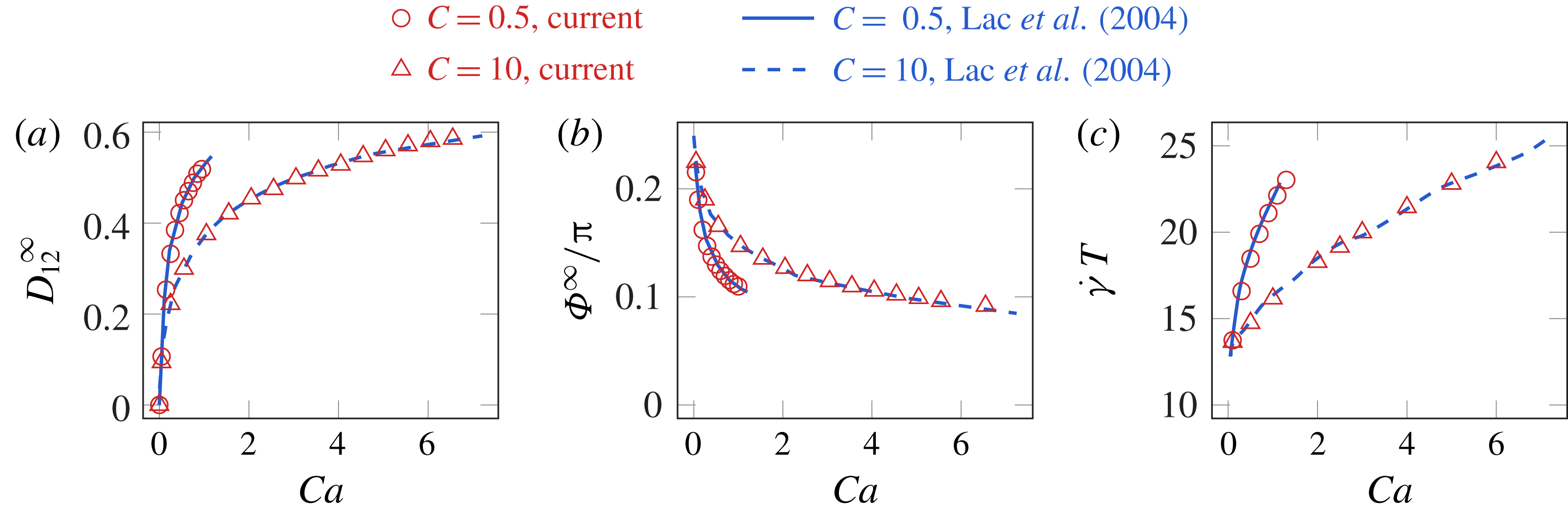
Comparison with Lac et al. (Reference Lac, Barthès-Biesel, Pelekasis and Tsamopoulos2004) for
 $a/b=1$
and
 $Ca$
and
 $C$
as indicated: (a) Taylor parameter, (b) inclination angle and (c) rotation period (see text).

Figure 2 shows that
 $D_{12}^{\infty }$
,
 $\unicode[STIX]{x1D6F7}^{\infty }$
and
 $T$
match closely with those of Lac et al. (Reference Lac, Barthès-Biesel, Pelekasis and Tsamopoulos2004). For this comparison, we do not include membrane bending resistance (
 $E_{b}=0$
), consistent with their simulations. As a result, the capsule membrane buckles (Walter et al.
Reference Walter, Rehage and Leonhard2001; Lac et al.
Reference Lac, Barthès-Biesel, Pelekasis and Tsamopoulos2004; Barthès-Biesel Reference Barthès-Biesel2009; Foessel et al.
Reference Foessel, Walter, Salsac and Barthès-Biesel2011) and forms features at the scale of the numerical discretization. As such, it is potentially sensitive to the mesh (Barthès-Biesel Reference Barthès-Biesel2009; Dupont et al.
Reference Dupont, Delahaye, Barthès-Biesel and Salsac2016). However, such sensitivity is not seen in figure 2 for a spherical capsule, where the results of our dealiased spectral method match those of the finite-element description (Lac et al.
Reference Lac, Barthès-Biesel, Pelekasis and Tsamopoulos2004).
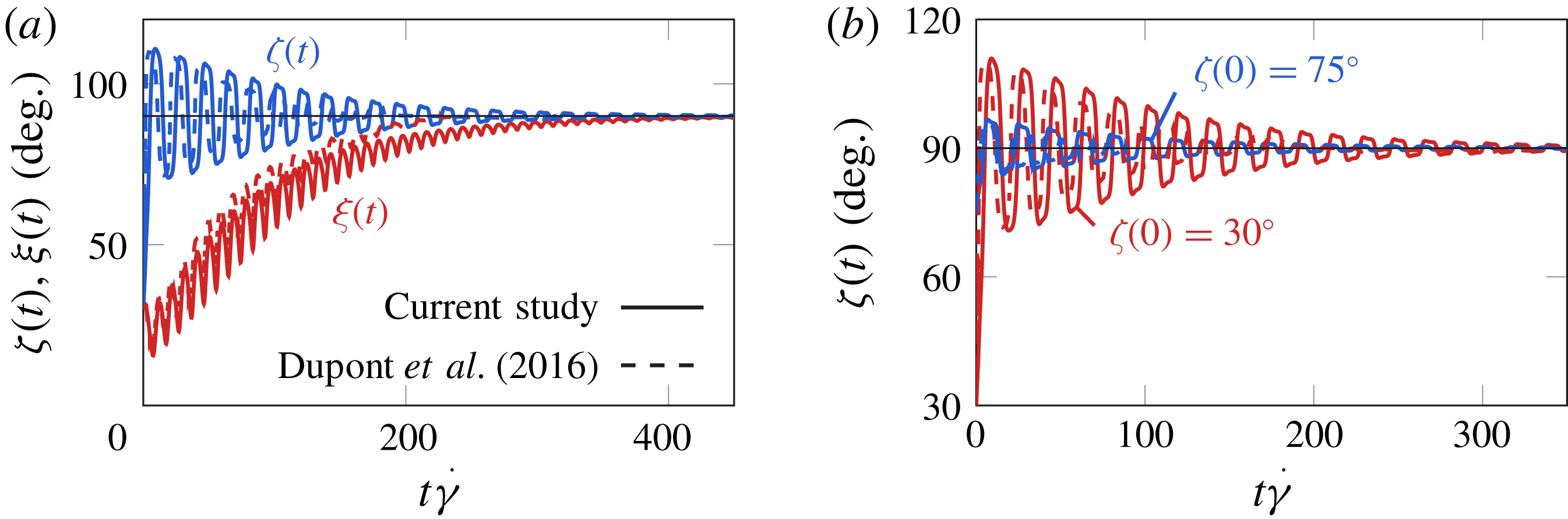
Cases with
 $a/b=0.5$
,
 $C=1$
,
 $E_{b}=0$
and
 $Ca=0.3$
: (a)
 $\unicode[STIX]{x1D709}(0)=\unicode[STIX]{x1D701}(0)=30^{\circ }$
and (b)
 $\unicode[STIX]{x1D701}(0)=30^{\circ }$
and
 $75^{\circ }$
.

Oblate capsules with
 $a/b=0.5$
will also be considered as reference configurations for the subsequent stability analysis, and they are compared with the results of Dupont et al. (Reference Dupont, Delahaye, Barthès-Biesel and Salsac2016) in figure 3. The evolving principal axis angles
 $\unicode[STIX]{x1D709}(t)$
and
 $\unicode[STIX]{x1D701}(t)$
are qualitatively similar to their reported results. However, for
 $t\dot{\unicode[STIX]{x1D6FE}}\gtrsim 400$
, our results approach the same
 $\unicode[STIX]{x1D701}=\unicode[STIX]{x1D709}=90^{\circ }$
values. We hypothesize that the small differences for
 $t\dot{\unicode[STIX]{x1D6FE}}\lesssim 300$
are due to differences in the numerical methods, as the capsules do not resist bending and buckle with features with wavelengths comparable to the spatial discretization. As such, the numerical smoothing (or artificial membrane stiffness) at the length scales of the discretization, characteristic of finite-element methods, could explain the differences. The spherical harmonic basis functions and dealiasing procedure used here minimize numerical smoothing, although our method still truncates the spherical harmonic series at degree
 $N$
. We confirm that the presented
 $\unicode[STIX]{x1D701}(t)$
and
 $\unicode[STIX]{x1D709}(t)$
for
 $t\dot{\unicode[STIX]{x1D6FE}}\lesssim 300$
vary by less than
 $3\,\%$
on increasing to
 $N=10$
, and note that only the long-time behaviour is important for the primary objectives of our analysis. We also include finite
 $E_{b}$
in all subsequent calculations.
With agreement established with previous simulations, we focus on cases with
 $a/b=0.5$
,
 $C=1$
, and
 $Ca$
ranging from 0.01 to 5, commensurate with previous empirical studies of capsule stability (Dupont et al.
Reference Dupont, Delahaye, Barthès-Biesel and Salsac2016). Our small
 $E_{b}=5\times 10^{-3}E_{s}r_{o}^{2}$
is both realistic and suppresses short-wavelength buckling, consistent with the absence of buckling reported in experimental observations (Barthès-Biesel Reference Barthès-Biesel2009). It also provides a physical regularization that removes mesh dependence from the linear stability analysis (§ 5). We analyse capsules initiated with both
 $\unicode[STIX]{x1D701}(0)=\unicode[STIX]{x1D709}(0)=0^{\circ }$
and
 $\unicode[STIX]{x1D701}(0)=\unicode[STIX]{x1D709}(0)=90^{\circ }$
, which are anticipated fixed points of the capsule motion (Barthès-Biesel Reference Barthès-Biesel2016).
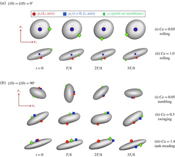
Visualizations of capsules over one half-period
 $T/2$
for
 $Ca$
as labelled and (a)
 $\unicode[STIX]{x1D701}(0)=\unicode[STIX]{x1D709}(0)=0^{\circ }$
and (b)
 $\unicode[STIX]{x1D701}(0)=\unicode[STIX]{x1D709}(0)=90^{\circ }$
. The
 $p_{\boldsymbol{x}}$
point is fixed on the membrane surface at
 $z=0$
.

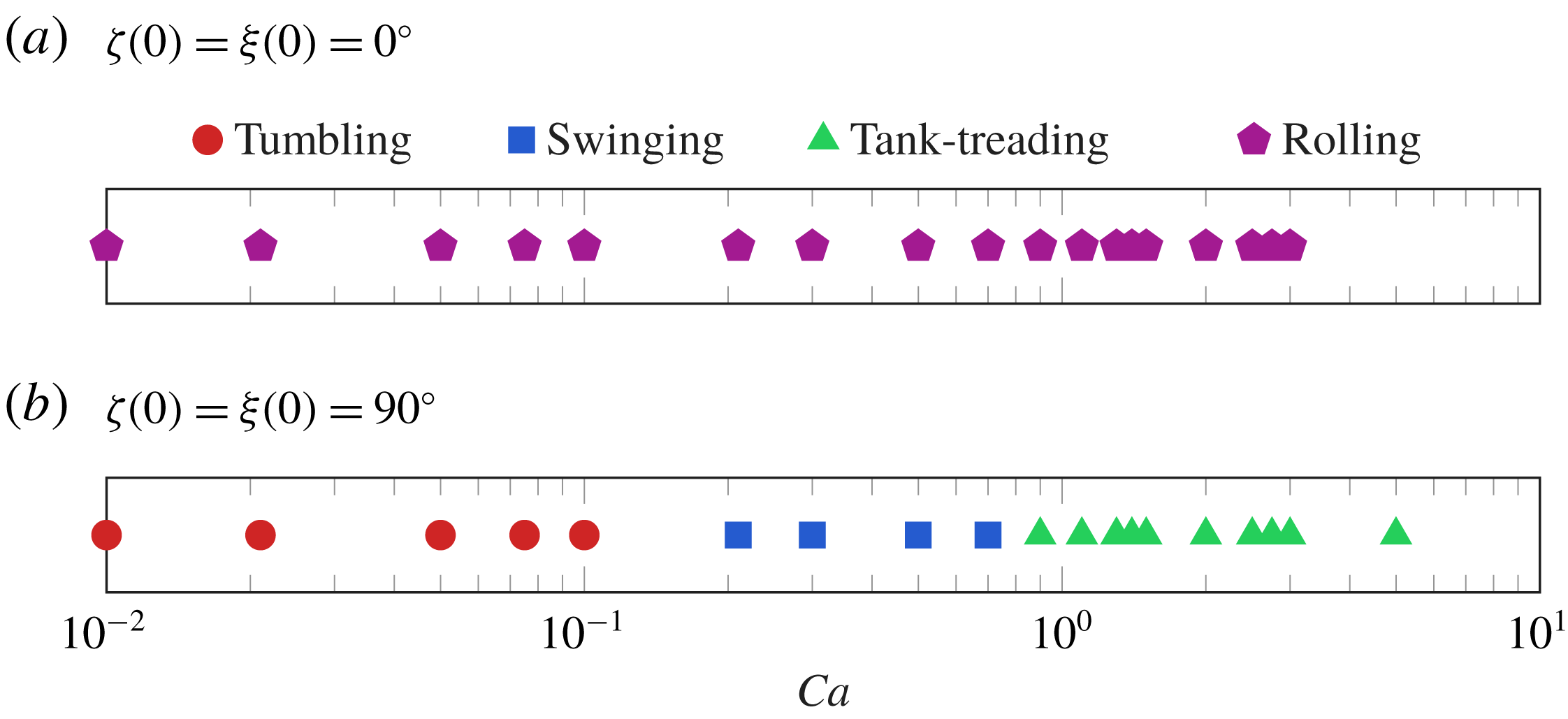
The base capsule motion is visualized for select cases in figure 4 and classified for the range of
 $Ca$
we consider in figure 5. The capsules tumble, swing, tank-tread or roll, as defined by Dupont et al. (Reference Dupont, Delahaye, Barthès-Biesel and Salsac2016). Capsules initiated with
 $\unicode[STIX]{x1D701}(0)=\unicode[STIX]{x1D709}(0)=0^{\circ }$
roll for all values of
 $Ca$
considered. In contrast, cases with
 $\unicode[STIX]{x1D701}(0)=\unicode[STIX]{x1D709}(0)=90^{\circ }$
have qualitatively different motion depending upon
 $Ca$
: for
 $Ca\lesssim 0.2$
, the capsule tumbles; for
 $0.2\lesssim Ca\lesssim 0.9$
, it swings; for
 $Ca\gtrsim 0.9$
, it tank-treads. For sufficiently large
 $Ca$
, the tank-treading behaviour is visually indistinguishable from a rolling motion, although it can be uniquely identified by tracking
 $p_{\unicode[STIX]{x1D709}}$
. These base flows are all time periodic per our specification, and as such are analysed with Floquet methods.
Base-flow capsule behaviour (see text) for
 $a/b=0.5$
,
 $C=1$
and initial orientations as labelled.

5 Floquet analysis formulation
The formulation is based upon that developed to analyse steadily flowing red blood cell trains (Bryngelson & Freund Reference Bryngelson and Freund2016, Reference Bryngelson and Freund2018), although here it is extended to include the time-periodic rotation of the capsule. In overview, the linearization proceeds by introducing
 $\unicode[STIX]{x1D739}[t]$
as a small perturbation to
 $\boldsymbol{s}[t]$
. Expansion of (3.3) and linearization yields
 $$\begin{eqnarray}\unicode[STIX]{x1D63C}[t]\unicode[STIX]{x1D739}[t]=\widetilde{\unicode[STIX]{x1D63D}}\{\boldsymbol{u}(\unicode[STIX]{x1D63D}\{\boldsymbol{s}[t]+\unicode[STIX]{x1D739}[t]\})-\boldsymbol{u}(\unicode[STIX]{x1D63D}\boldsymbol{s}[t])\}.\end{eqnarray}$$
A full-rank orthogonal set of perturbations
 $\unicode[STIX]{x1D739}_{i}$
are used sequentially to calculate each column
 $i$
of matrix
 $\unicode[STIX]{x1D63C}[t]$
at time
 $t$
. For the results presented, we take
 $\Vert \unicode[STIX]{x1D739}[t]\Vert =\unicode[STIX]{x1D6FF}=10^{-3}$
, and
 $\unicode[STIX]{x1D63C}[t]$
is evaluated at
 $j=1,\ldots ,N_{t}$
uniformly spaced times
 $t_{j}=(j-1)T/(N_{t}-1)$
with
 $N_{t}=10^{4}$
. Results are insensitive to these specific choices of numerical parameters. With
 $\unicode[STIX]{x1D63C}$
so determined, the evolution of any small perturbation to the spherical harmonic coefficients
 $\unicode[STIX]{x1D73A}[t]$
is then governed by
 $$\begin{eqnarray}\frac{\text{d}\unicode[STIX]{x1D73A}[t]}{\text{d}t}=\unicode[STIX]{x1D63C}[t]\unicode[STIX]{x1D73A}[t].\end{eqnarray}$$
Since
 $\unicode[STIX]{x1D63C}[t]$
is periodic, (5.2) is a canonical Floquet system with solution of the form
 $$\begin{eqnarray}\unicode[STIX]{x1D73A}[t]=\unicode[STIX]{x1D653}[t]\unicode[STIX]{x1D73A}_{o},\end{eqnarray}$$
where
 $\unicode[STIX]{x1D653}[t]$
is the fundamental solution matrix. Following usual procedures (e.g. Verhulst Reference Verhulst2006), we assume that
 $\unicode[STIX]{x1D73A}[t]$
has the form
 $$\begin{eqnarray}\unicode[STIX]{x1D73A}[t]=\mathop{\sum }_{i=1}^{3N^{2}}c_{i}\boldsymbol{p}_{i}[t]\exp \unicode[STIX]{x1D707}_{i}t,\end{eqnarray}$$
where
 $c_{i}$
are constants,
 $\unicode[STIX]{x1D707}_{i}$
are exponential growth rates and
 $\boldsymbol{p}_{i}[t]$
are unknown periodic functions. Periodicity requires
 $$\begin{eqnarray}\unicode[STIX]{x1D653}[t+T]=\unicode[STIX]{x1D653}[t]\unicode[STIX]{x1D653}^{-1}[0]\unicode[STIX]{x1D653}[T]=\unicode[STIX]{x1D653}[t]\unicode[STIX]{x1D63E},\end{eqnarray}$$
where
 $\unicode[STIX]{x1D63E}=\unicode[STIX]{x1D653}^{-1}[0]\unicode[STIX]{x1D653}[T]$
is the monodromy matrix (Liu Reference Liu2003; Verhulst Reference Verhulst2006). Substitution of (5.3) into (5.2) yields a system to be solved for
 $\unicode[STIX]{x1D653}[t]$
,
 $$\begin{eqnarray}\frac{\text{d}\unicode[STIX]{x1D653}[t]}{\text{d}t}=\unicode[STIX]{x1D63C}[t]\unicode[STIX]{x1D653}[t].\end{eqnarray}$$
A key to Floquet analysis is that the stability properties can be determined independently of the initial condition
 $\unicode[STIX]{x1D653}[0]$
(Liu Reference Liu2003; Verhulst Reference Verhulst2006); we follow the usual practice of selecting identity
 $\unicode[STIX]{x1D653}[t_{1}=0]=\unicode[STIX]{x1D644}$
, so
 $\unicode[STIX]{x1D63E}=\unicode[STIX]{x1D653}[T]$
is the principal fundamental matrix. In our calculations,
 $\unicode[STIX]{x1D653}[t_{N_{t}}=T]$
, and thus
 $\unicode[STIX]{x1D63E}$
, is found by integrating (5.6). For this, we use the trapezoidal rule
 $(2\unicode[STIX]{x1D644}-\unicode[STIX]{x0394}t\unicode[STIX]{x1D63C}[t_{j+1}])\unicode[STIX]{x1D653}[t_{j+1}]=(2\unicode[STIX]{x1D644}+\unicode[STIX]{x0394}t\unicode[STIX]{x1D63C}[t_{j}])\unicode[STIX]{x1D653}[t_{j}]$
, which preserves time reversibility and thus does not introduce numerical dissipation. The eigenvalues
 $\unicode[STIX]{x1D70C}_{i}=\exp \unicode[STIX]{x1D707}_{i}T$
of
 $\unicode[STIX]{x1D63E}$
are the Floquet multipliers, the factors by which
 $\Vert \unicode[STIX]{x1D73A}[t]\Vert$
for component
 $i$
of (5.4) grows or decays over a period. Components with
 $|\unicode[STIX]{x1D70C}_{i}|>1$
are unstable.
6 Results
We first consider the
 $a/b=0.5$
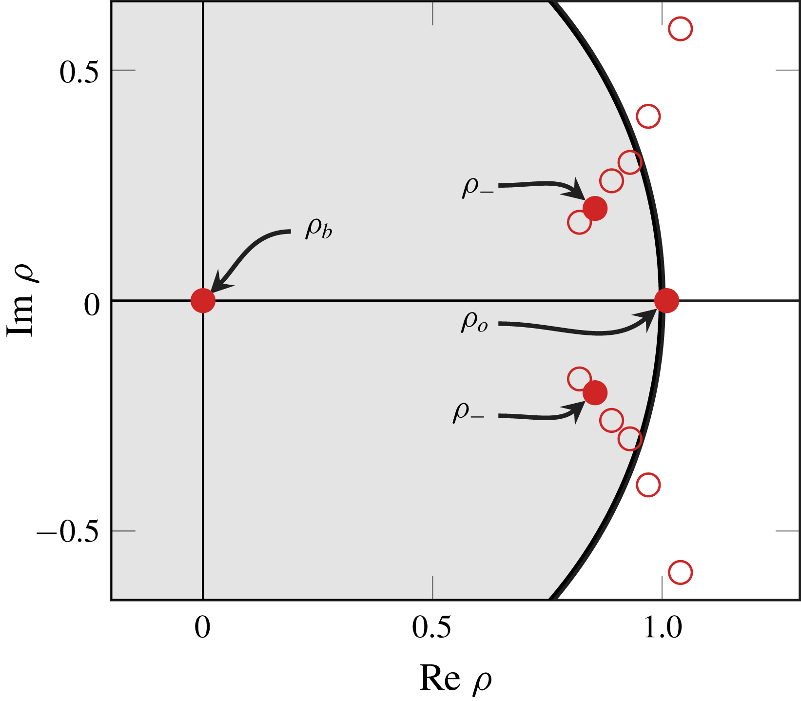
capsules of § 4, example Floquet multipliers for which are shown in figure 6. There is a complex conjugate pair of modestly stable multipliers
 $|\unicode[STIX]{x1D70C}_{-}|=0.84$
, which decay over many periods of the rotating capsule motion, and a neutrally stable multiplier
 $\unicode[STIX]{x1D70C}_{o}=1$
; these have associated eigenvectors
 $\boldsymbol{v}_{-}$
and
 $\boldsymbol{v}_{o}$
respectively. Neutrally stable multipliers are only determined within the accuracy of our calculations, which for this case is within
 $\unicode[STIX]{x1D70C}_{o}=1\pm 10^{-2}$
. This is a result of the approximations introduced by the finite
 $\unicode[STIX]{x1D6FF}$
used when constructing
 $\unicode[STIX]{x1D63C}$
, the discretization of
 $\unicode[STIX]{x1D63C}[t]$
in time, and the convergence of the periodic base-flow motion; the coupling between these errors makes quantification of their relative importance challenging, although the details of the coupling are not directly relevant to the conclusions of this paper. For example, if the nominally neutral modes were in fact mildly unstable within this constraint, they would require
 $t>700T$
– over 700 periods of rotation – to amplify by a linear mechanism from an initial perturbation amplitude
 $\hat{\unicode[STIX]{x1D700}}=10^{-3}$
to unity. Thus, this accuracy is taken to be sufficient to support our conclusions. All other Floquet multipliers of figure 6 are very stable and have
 $|\unicode[STIX]{x1D70C}|\approx 0$
, with their associated perturbations vanishing (within the accuracy of our methods) well before a single period
 $T$
.
The spectrum of
 $\unicode[STIX]{x1D63E}$
for
 $a/b=0.5$
,
 $C=1$
,
 $Ca=1.4$
and
 $\unicode[STIX]{x1D709}(0)=0^{\circ }$
. The
 $\unicode[STIX]{x1D70C}$
are categorized as neutrally (
 $\unicode[STIX]{x1D70C}_{o}$
), modestly (
 $\unicode[STIX]{x1D70C}_{-}$
) or very (
 $\unicode[STIX]{x1D70C}_{b}$
) stable (see text). Open symbols are
 $\unicode[STIX]{x1D70C}_{-}$
for
 $Ca$
between 0.5 and 2.

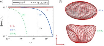
(a) Linear prediction and DNS for an initial condition (i.c.) associated with the eigenvectors of example Floquet multipliers as labelled for several
 $T$
periods for
 $a/b=0.5$
,
 $C=1$
,
 $Ca=1.4$
and
 $\unicode[STIX]{x1D709}(0)=0^{\circ }$
. The
 $t=T$
point is indicated by a dotted line. (b) The corresponding eigenvectors (ii)
 $\boldsymbol{v}_{-}$
and (iii)
 $\boldsymbol{v}_{b}$
, magnified as
 $\boldsymbol{s}[0]+5\boldsymbol{v}$
for visualization.

Figure 7(a) confirms agreement between the linear theory and DNS for the
 $\boldsymbol{v}_{o}$
and
 $\boldsymbol{v}_{-}$
modes, which serves as a verification of our procedures. We also include one of the
 $|\unicode[STIX]{x1D70C}|\approx 0$
modes, labelling it
 $\boldsymbol{v}_{b}$
, and confirm that it decays so fast that the finite precision of the calculations make it impossible to confirm its specific behaviour at the end of a
 $T$
period. The
 $\unicode[STIX]{x1D70C}_{b}$
are thus unimportant for multiperiod behaviour.
The eigenvector
 $\boldsymbol{v}_{-}$
, visualized in figure 7(bii), is a tilt of the capsule about the
 $\boldsymbol{e}_{y}$
axis, and, in contrast, the
 $\boldsymbol{v}_{b}$
is a shorter-wavelength deformation of the capsule. We anticipate the rapid decay of
 $\boldsymbol{v}_{b}$
to be due to viscously damped elastic recovery. The decay rate of elastic perturbations can be estimated in the absence of shear flow to decay by more than a factor of 100 over time
 $T$
(Rochal, Lorman & Mennessier Reference Rochal, Lorman and Mennessier2005; Zhao et al.
Reference Zhao, Isfahani, Olson and Freund2010), matching our observations. The eigenvector
 $\boldsymbol{v}_{o}$
is simply an advancement of the capsule surface in the rolling direction, and thus its neutral stability is expected. As such, we focus upon
 $\boldsymbol{v}_{-}$
.
Floquet multiplier
 $|\unicode[STIX]{x1D70C}_{-}|$
for the full range of
 $Ca$
,
 $a/b=0.5$
and 0.6, and (a)
 $\unicode[STIX]{x1D709}(0)=0^{\circ }$
and (b)
 $\unicode[STIX]{x1D709}(0)=90^{\circ }$
. The vertical lines indicate ——
 $Ca_{c}^{(1)}$
and – – –
 $Ca_{c}^{(2)}$
(see text).

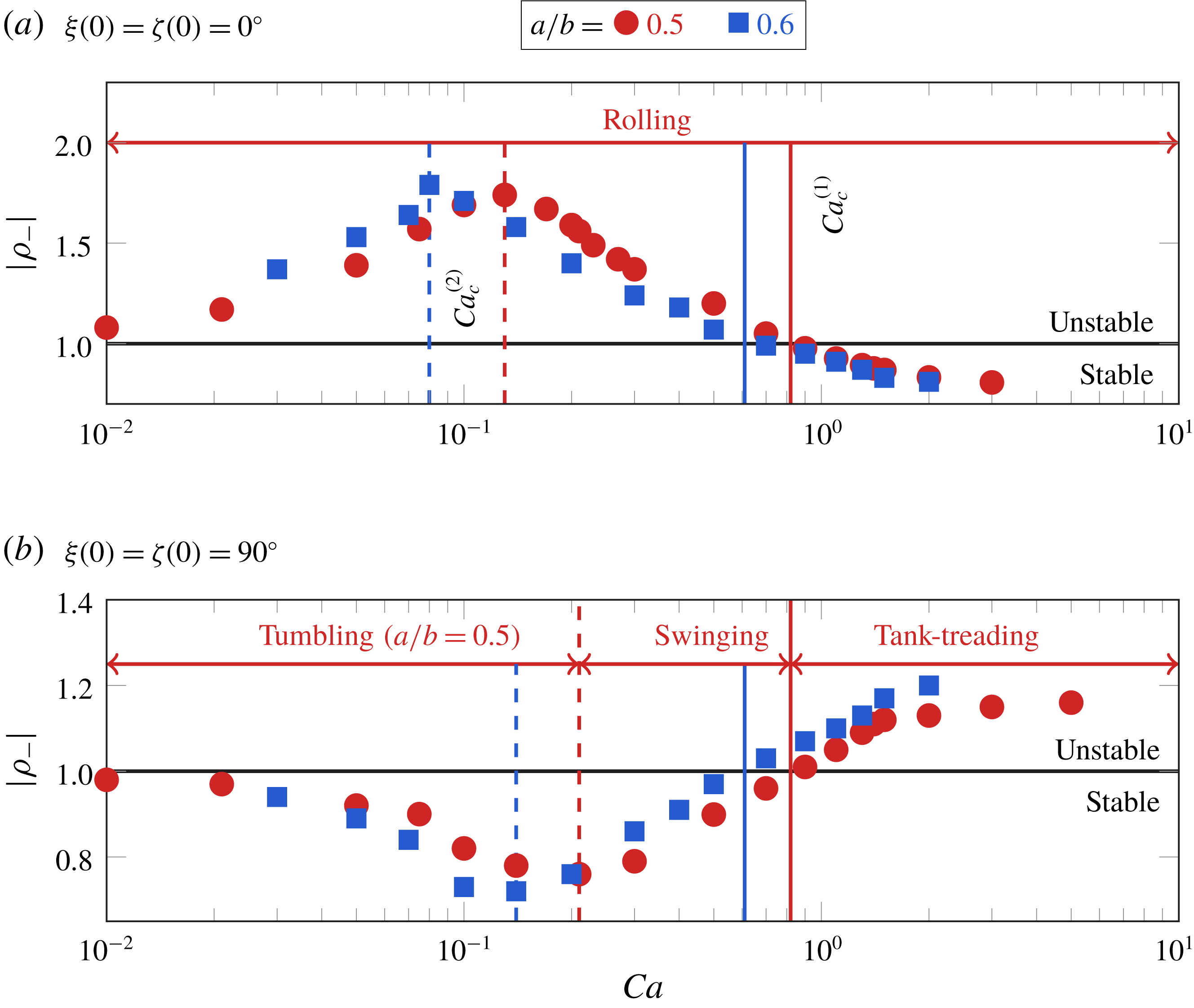
For the full range of
 $Ca$
, for both orientations and aspect ratios, each case has one and only one
 $\unicode[STIX]{x1D70C}_{-}$
-like complex conjugate pair of Floquet multipliers; these
 $|\unicode[STIX]{x1D70C}_{-}|$
are shown in figure 8. A least-squares quadratic fit of the five values closest to
 $|\unicode[STIX]{x1D70C}_{-}|=1$
gives a critical value of
 $Ca_{c}^{(1)}=0.82$
for the stable–unstable transition for
 $a/b=0.5$
, and correspondingly
 $Ca_{c}^{(1)}=0.61$
for
 $a/b=0.6$
. This is consistent with the trend noted by Dupont et al. (Reference Dupont, Delahaye, Barthès-Biesel and Salsac2016), who observed stable swinging at larger
 $Ca$
for smaller
 $a/b$
. The
 $\unicode[STIX]{x1D70C}_{-}$
are complex at
 $|\unicode[STIX]{x1D70C}_{-}|=1$
, as shown in figure 6; this is indicative of a subcritical Neimark–Sacker bifurcation, for which a spiral fixed point changes stability and produces a limit cycle (Sacker Reference Sacker1964). We note that while the bifurcation is clear, the
 $\boldsymbol{v}_{-}$
shape and the perturbed velocity field do not qualitatively change near
 $Ca_{c}^{(1)}$
.
For
 $\unicode[STIX]{x1D709}(0)=0^{\circ }$
, the rolling motion is unstable for
 $Ca<Ca_{c}^{(1)}$
, with
 $|\unicode[STIX]{x1D70C}_{-}|$
increasing with
 $Ca$
for
 $Ca<Ca_{c}^{(2)}$
, where
 $Ca_{c}^{(2)}=0.13$
for
 $a/b=0.5$
and
 $Ca_{c}^{(2)}=0.08$
for
 $a/b=0.6$
. It otherwise decreases with
 $Ca$
. For
 $Ca>Ca_{c}^{(1)}$
,
 $|\unicode[STIX]{x1D70C}_{-}|<1$
indicates stable rolling. This behaviour reverses for
 $\unicode[STIX]{x1D709}(0)=90^{\circ }$
in figure 8(b), where we see that the tumbling and swinging motions of
 $Ca<Ca_{c}^{(1)}$
are stable, with
 $|\unicode[STIX]{x1D70C}_{-}|$
decreasing with
 $Ca$
in the tumbling regime (
 $Ca<Ca_{c}^{(2)}$
, where in this case
 $Ca_{c}^{(2)}=0.21$
for
 $a/b=0.5$
and
 $Ca_{c}^{(2)}=0.14$
for
 $a/b=0.6$
). For
 $Ca>Ca_{c}^{(1)}$
, we have
 $|\unicode[STIX]{x1D70C}_{-}|>1$
, so tank treading is unstable. For very small
 $Ca<0.01$
,
 $|\unicode[STIX]{x1D70C}_{-}|\rightarrow 1$
for both the tumbling and rolling motions, even as the period
 $T$
becomes larger, suggesting that in the
 $Ca\rightarrow 0$
limit, both are neutrally stable. The stability of the tumbling and swinging motions, as well as the large-
 $Ca$
rolling motion, matches the observed long-time behaviour (Wang et al.
Reference Wang, Sui, Spelt and Wang2013; Dupont et al.
Reference Dupont, Delahaye, Barthès-Biesel and Salsac2016), which confirms that nothing was missed by these more empirically grounded studies.
7 Discussion and conclusions
The Floquet analysis was designed to quantify (and clarify) the long-time behaviour of capsules in viscous shear flow, motivated in part by the challenges of performing and interpreting corresponding long-time simulations. This has not before been undertaken for this flow. For all cases, most Floquet multipliers are nondescript membrane deformations that rapidly decay with
 $|\unicode[STIX]{x1D70C}|\ll 1$
, and thus dissipate within one period of the base capsule motion. This is also consistent with observations of actual capsules, which can rapidly achieve a cyclic behaviour (Walter et al.
Reference Walter, Rehage and Leonhard2001). An expected neutrally stable mode corresponding to a simple rotation of the capsule surface in the flow direction was likewise found. The most interesting mode was the
 $\unicode[STIX]{x1D70C}_{-}$
complex conjugate pair, which decays or grows over several periods. A single such pair was identified for every set of parameters in the ranges evaluated, although there has not yet been a formal or extensive search for other possible behaviour for other configurations. In all cases, stability was quantified as it depends upon
 $Ca$
, aspect ratio
 $a/b$
and the initial capsule orientation
 $\unicode[STIX]{x1D709}(0)$
, with the stable cases matching the long-time behaviour previously observed.
Our stability formulation is perturbation based and includes coupling between a full-rank set of perturbations and the base flow, so its construction is relatively expensive even for simple flows. Data-driven methods, such as those utilizing dynamic mode decompositions (Schmid Reference Schmid2010; Bagheri Reference Bagheri2013; Pumhössel, Hehenberger & Zeman Reference Pumhössel, Hehenberger and Zeman2014) or Koopman operator techniques (Rowley et al. Reference Rowley, Mezic, Bagheri, Schlatter and Henningson2009; Bagheri Reference Bagheri2013), have proved useful if a base flow is unavailable or full construction of the linear stability analysis is prohibitively expensive. These methods determine the most unstable growth rate through a series of temporal realizations of the evolution to disordered flow. Often, only a relatively small number of such realizations is required, making such analysis computationally efficient. Further, direct computation of perturbations to the flow, or construction of an accurate base flow, is not required. However, such analyses cannot quantify the decay rate for a full-rank set of perturbations to the system, since the dynamics is dominated by the most unstable flow behaviour. Although the information they supply is thus limited, we expect that such methods might be particularly useful for large systems, such as many-capsule flows. Of course, advancement in computational capabilities will also facilitate larger-scale direct analyses and perhaps facilitate the discovery of still richer behaviour.
While the formulation presented here was limited to time-periodic base flows, methods for relaxing this restriction to time-general flows exist, although they are challenging since they do not admit the simplifications of Floquet’s theorem. They typically either require analysis of the fundamental matrix operator directly over long times through a singular-value decomposition (Schmid & Kytomaa Reference Schmid and Kytomaa1994; Schmid & Henningson Reference Schmid and Henningson2012) or utilize adjoint operators through an inverse process known as adjoint looping (Juniper Reference Juniper2011). Such analyses are generally more computationally expensive than those for the analogous time-stationary or time-periodic flows, although they are potentially tractable with the methods presented here. Extension of our formulation in this respect would then be appropriate for any non-time-periodic capsule flow, such as that of biconcave capsules in sufficiently strong steady (Skotheim & Secomb Reference Skotheim and Secomb2007) or oscillatory shear flow (Dupire, Abkarian & Viallat Reference Dupire, Abkarian and Viallat2010), or single vesicles flowing in narrow confines (Aouane et al. Reference Aouane, Thiébaud, Benyoussef, Wagner and Misbah2014).
Acknowledgement
This work was supported in part by the National Science Foundation under grant no. CBET 13-36972.