1 Introduction and background
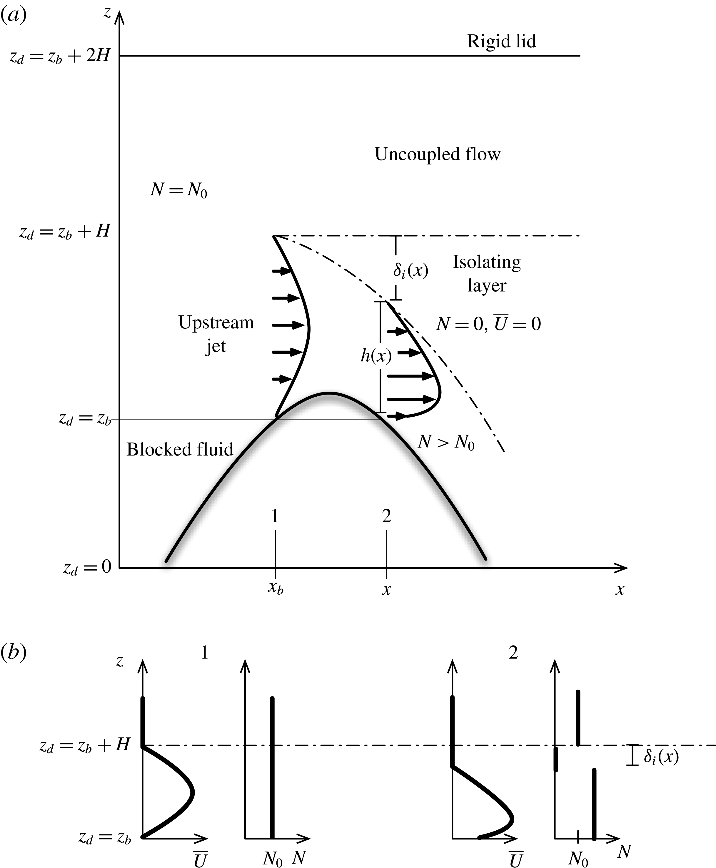
Features reminiscent of shear induced instability are often seen in the lee of topographically controlled stratified flows in the atmosphere and ocean. Despite a wealth of literature on the subject (e.g. Scinocca & Peltier Reference Scinocca and Peltier1989; Smith Reference Smith1991; Farmer & Armi Reference Farmer and Armi1999; Armi & Mayr Reference Armi and Mayr2007 and references contained therein), the origin of these instabilities and their growth rate remain uncertain. Our aim here is to better reconcile field observations with results from numerical simulations exhibiting these features and linear stability theory. Figure 1 shows the idealized spatial structure of the flows under consideration; see also Winters & Armi (Reference Winters and Armi2014). A jet-like upstream profile with constant stratification
 $N_{0}$
develops into a strong thinning downslope flow beneath a layer of nearly stagnant mixed fluid also known as the isolating layer. This downstream evolution is associated with intensifying shear at the interface between the flowing and stagnant layers. A feature to note is the upstream influence, characterized, in part, by stagnant ‘blocked’ fluid below the vertical level
 $z_{d}=z_{b}$
. The subscript
 $d$
indicates that this is a dimensional quantity and is used to avoid confusion with non-dimensional coordinates which are introduced later. For a topography with crest height
 $h_{0}$
, blocking is achieved by the upstream propagation of internal waves with vertical scale of approximately
 $h_{0}$
. Given a far upstream velocity
 $U_{\infty }$
, mountain height
 $h_{0}$
and uniform upstream stratification
 $N_{0}$
, our primary focus is in the flow regime
 $$\begin{eqnarray}U_{\infty }/N_{0}h_{0}\ll 1,\end{eqnarray}$$
where upstream influence and blocking are important.
(a) The downslope jet setting where the flow configurations described occur. Here,
 $z_{d}=z_{b}$
is the dimensional vertical level below which the fluid is blocked;
 $N$
is the background stratification and
 $\bar{U}$
is the background fluid velocity;
 $\unicode[STIX]{x1D6FF}_{i}(x)$
denotes the thickness of the motionless and homogeneous isolating layer as a function of downstream distance. (b) The typical velocity and stratification profiles at the blocking point and an arbitrary point downstream of the crest, labelled 1 and 2 respectively.

Observations of the 1972 Boulder storm by Lilly (Reference Lilly1978) revealed quasiperiodic oscillations in the lee of the topography which were conjectured to be signatures of unstable Kelvin–Helmholtz (K–H) waves. While Clark & Farley (Reference Clark and Farley1984) held these to be the result of a three-dimensional (3D) shear-aligned convective instability, Scinocca & Peltier (Reference Scinocca and Peltier1989) contested this view and instead advanced the idea that the dynamic instability of downslope windstorms is an intrinsically two-dimensional (2D) phenomenon. In support of this assertion, they were able to replicate the quasiperiodic 5–15 min pulses revealed in the data using a 2D nonlinear non-hydrostatic anelastic numerical model. To investigate the effect of the upstream conditions on this phenomenon, they also simulated a downslope windstorm with an initially uniform upstream profile and found that the time evolution of the solution clearly exhibited upstream influence, characterized principally by blocking, as well as the pulsating features alluded to above. This led them to conclude that the occurrence of the pulsations does not depend sensitively on 3D effects or on upstream conditions that precipitate the downslope windstorm. More recently, detailed measurements by Beluši’c, Pasarić & Orlić (Reference Beluši’c, Pasarić and Orlić2004) confirmed the presence of 3–13 min pulsations in the dynamically similar downslope Bora flow as well.
To test the hypothesis that these pulsations are the result of a dynamic instability of the mean flow, Peltier & Scinocca (Reference Peltier and Scinocca1990) performed a spatial and temporal stability analysis of the downstream flow solutions of Scinocca & Peltier (Reference Scinocca and Peltier1989) but found that the growth rates obtained were almost two orders of magnitude smaller than expected. They conjectured that the mean state extracted from the numerical simulation had already been modified by nonlinear interactions with the instability modes. This motivated them to reperform the stability analysis after introducing plausible but rather ad hoc changes to the base state. Only then were they able to obtain growth rates that matched their 2D simulations. Here, we will examine the stability of profiles whose essential character is similar to the modified profiles of Peltier & Scinocca (Reference Peltier and Scinocca1990), but determined by recently obtained solutions for steady density-stratified topographically controlled flows by Winters & Armi (Reference Winters and Armi2014).
A similar (to our) approach was adopted by Smith (Reference Smith1985). However, he assumed a uniform upstream profile and invoked Long’s (Reference Long1955) equation, streamline bifurcation and local hydraulic theory to produce a downslope flow underlying a stagnant uniform-density layer aloft. Focusing only on the flowing layer, he noted that if the Miles–Howard condition (Howard Reference Howard1961; Miles Reference Miles1961) of Richardson number,
 $Ri<1/4$
is considered to be a sufficient criterion for onset of instability, then the local hydraulic theory prediction is validated by the Scinocca & Peltier (Reference Scinocca and Peltier1989) numerical simulation of idealized severe downslope windstorms. To test whether this agrees with results from linear stability theory, Smith (Reference Smith1991) solved the Taylor–Goldstein equation at a number of downstream locations for the base flow configurations of Smith (Reference Smith1985). We note, however, that in his analysis, the background states were truncated at the upper edge of the flowing layer so as to exclude the stagnant uniform-density isolating layer aloft. The stability analysis for these profiles, while yielding values for the wavelength that were consistent with Scinocca & Peltier (Reference Scinocca and Peltier1989), severely underpredicted the onset and growth rate of the unstable K–H mode. Further, his choice of a uniform upstream profile excludes blocking and is not applicable in flow regimes where blocking and upstream influence are dynamically important. Thus, linear stability analysis for flow profiles both produced by local hydraulic theory and extracted from numerical simulations yielded very small growth rates that were insensitive to upstream influence.
Recently, Winters & Armi (Reference Winters and Armi2014) accounted for the upstream influence of the topography in constructing optimally controlled jet-like solutions that thin and accelerate over the crest. These solutions are valid in the asymptotic limit of (1.1) and are characterized by a blocked region underlying the jet, a stagnant isolating layer of uniform density and a bifurcating streamline that separates the accelerating flow below from the dynamically uncoupled flow aloft (cf. figure 1). They then showed that, downstream of the blocking location, there emerges a region of subquarter Richardson number along the upper edge of the active layer, increasing in thickness downstream, and surmised that this suggests an environment conducive to the generation of shear instability.
One of our objectives here is to investigate the stability of the profiles produced in the optimally controlled flow of Winters & Armi (Reference Winters and Armi2014) at different downstream locations. These profiles have the character that the fluid velocity is zero in the overlying isolating layer, the thickness of which increases downstream of the crest. Formally, we will examine flow profiles characteristic of low-Froude-number settings.
2 Ambient profiles characteristic of controlled downslope flows
The family of profiles we study are those that arise naturally in the lee of the topography when the problem is formulated within a hydraulic framework as in Winters & Armi (Reference Winters and Armi2014). Figure 1 introduces our notation and illustrates the setting in which these flow configurations are encountered. At any downstream location
 $x>x_{b}$
, the essential features of such flows are the following.
-
(i) The profile is jet-like, with an overlying stagnant region whose thickness,
 $\unicode[STIX]{x1D6FF}_{i}$
, depends on the downstream position
$x$
.
-
(ii) Moving downstream, the velocity maximum descends from its initial vertical level.
-
(iii) The volumetric flow rate
$Q$
is conserved and is equal to the value associated with the upstream jet. -
(iv) As the flowing layer thins, the density difference remains the same. This implies a proportionately stronger stratification, which we take to be uniform for simplicity. This is a good approximation to the exact solution shown in figure 10 of Winters & Armi (Reference Winters and Armi2014).


The upstream profile is a parabolic jet with an overlying dynamically uncoupled layer, each of height
 $H$
for simplicity. The upstream buoyancy frequency is constant and equal to
 $N_{0}$
. As the flow develops, at each downstream location, it remains quasi-jet-like, but with a reduced thickness
 $h=H-\unicode[STIX]{x1D6FF}_{i}$
, a stronger stratification and an isolating layer of height
 $\unicode[STIX]{x1D6FF}_{i}$
. The volumetric flow rate,
 $Q=(2/3)U_{0}H$
, upstream remains conserved. To include the possibility of an accelerating bottom streamline, we represent the flow mathematically as a superposition of a parabolic jet with maximum
 $U_{\unicode[STIX]{x1D6FF}_{i}}$
and a linear component that vanishes at
 $z_{b}+h$
. We define
 $$\begin{eqnarray}u_{b}=\unicode[STIX]{x1D6FD}U_{\unicode[STIX]{x1D6FF}_{i}},\end{eqnarray}$$
where
 $u_{b}$
is the velocity of the bottom streamline. The velocity and density profiles are then given by
 $$\begin{eqnarray}\displaystyle & \displaystyle \bar{U}_{d}(z_{d})=\left\{\begin{array}{@{}ll@{}}0,\quad & z_{b}+h\leqslant z_{d}\leqslant z_{b}+2H,\\ \displaystyle 4U_{\unicode[STIX]{x1D6FF}_{i}}\left[\frac{z_{d}}{h}-\left(\frac{z_{d}}{h}\right)^{2}\right]+\frac{\unicode[STIX]{x1D6FD}U_{\unicode[STIX]{x1D6FF}_{i}}}{h}(h-z_{d}),\quad & z_{b}\leqslant z_{d}\leqslant z_{b}+h,\end{array}\right.\quad (\text{m}~\text{s}^{-1}) & \displaystyle \nonumber\\ \displaystyle & & \displaystyle\end{eqnarray}$$
 $$\begin{eqnarray}\displaystyle & \displaystyle \bar{\unicode[STIX]{x1D70C}}_{d}(z_{d})=\left\{\begin{array}{@{}ll@{}}\displaystyle \unicode[STIX]{x1D70C}_{0}+\unicode[STIX]{x0394}\unicode[STIX]{x1D70C}-\frac{\unicode[STIX]{x0394}\unicode[STIX]{x1D70C}}{2h}z_{d},\quad & z_{b}\leqslant z_{d}\leqslant z_{b}+h,\\ \displaystyle \unicode[STIX]{x1D70C}_{0}+\frac{\unicode[STIX]{x0394}\unicode[STIX]{x1D70C}}{2},\quad & z_{b}+h\leqslant z_{d}\leqslant z_{b}+H,\\ \displaystyle \unicode[STIX]{x1D70C}_{0}+\frac{\unicode[STIX]{x0394}\unicode[STIX]{x1D70C}}{2}-\frac{\unicode[STIX]{x0394}\unicode[STIX]{x1D70C}}{2H}(z_{d}-H),\quad & z_{b}+H\leqslant z_{d}\leqslant z_{b}+2H,\end{array}\right.\quad (\text{kg}~\text{m}^{-3}) & \displaystyle \nonumber\\ \displaystyle & & \displaystyle\end{eqnarray}$$
where the overbar is used to denote the background flow field and the subscript ‘
 $d$
’ indicates dimensional quantities. It should be noted that
 $Q$
conservation and the bottom velocity parameter
 $\unicode[STIX]{x1D6FD}$
jointly determine the parabolic maximum
 $U_{\unicode[STIX]{x1D6FF}_{i}}$
at any given downstream position as
 $$\begin{eqnarray}\frac{2}{3}U_{0}H=U_{\unicode[STIX]{x1D6FF}_{i}}h\left(\frac{2}{3}+\frac{\unicode[STIX]{x1D6FD}}{2}\right).\end{eqnarray}$$
Incorporation of a perfectly homogeneous isolating layer introduces a discontinuity in the derivatives of the velocity and density at
 $h(x)$
. To smooth this, we take these profiles as initial conditions for a one-dimensional (1D) heat equation and allow diffusion for just enough time that the edge discontinuity is ‘sufficiently’ ironed out for numerical discretization purposes. We have checked that our results are only weakly sensitive to small changes in the amount of smoothing. For example, the growth rate differed by only
 ${\approx}1\,\%$
when the discontinuities were smoothed over a distance
 $h/50$
versus
 $h/200$
. Similarly, the difference in growth rate was less than 2 % when the ratio of the density and velocity diffusivity parameters was varied between 1 and 10.
For this problem, it is convenient to introduce another parameter,
 $$\begin{eqnarray}\unicode[STIX]{x1D6FC}=\frac{h}{H}=\frac{H-\unicode[STIX]{x1D6FF}_{i}}{H},\end{eqnarray}$$
which gives the height of the flowing layer as a fraction of the upstream thickness. The generalized stability analysis is then carried out in a two-parameter space of
 $\unicode[STIX]{x1D6FC}$
and the bottom boundary parameter
 $\unicode[STIX]{x1D6FD}$
, defined in (2.1). For the optimal flow solutions of Winters & Armi (Reference Winters and Armi2014), this reduces to a one-parameter space since there is a unique
 $\unicode[STIX]{x1D6FD}$
that produces the best fit to the actual velocity profile for each
 $\unicode[STIX]{x1D6FC}$
. We will examine this particular problem in more detail in § 6.2.
3 Mathematical formulation of the streamwise-local stability problems
The stability problem is developed using the primitive variable formulation and the normal mode decomposition. We begin with the inviscid Boussinesq equations of motion in non-dimensional form,
 $$\begin{eqnarray}\displaystyle & \displaystyle \frac{\text{D}\boldsymbol{u}}{\text{D}t}+J\unicode[STIX]{x1D70C}\hat{\boldsymbol{k}}=-\unicode[STIX]{x1D735}p, & \displaystyle\end{eqnarray}$$
 $$\begin{eqnarray}\displaystyle & \displaystyle \frac{\text{D}\unicode[STIX]{x1D70C}}{\text{D}t}=0, & \displaystyle\end{eqnarray}$$
 $$\begin{eqnarray}\displaystyle & \displaystyle \unicode[STIX]{x1D735}\boldsymbol{\cdot }\boldsymbol{u}=0, & \displaystyle\end{eqnarray}$$
 $\boldsymbol{u}$
denotes the velocity vector,
 $p$
and
 $\unicode[STIX]{x1D70C}$
the pressure and density field respectively and
 $\hat{\boldsymbol{k}}$
is a unit vector oriented along the positive
 $z$
axis.
 $$\begin{eqnarray}J=g\frac{\unicode[STIX]{x0394}\unicode[STIX]{x1D70C}}{\unicode[STIX]{x1D70C}_{0}}\frac{h}{U_{max}^{2}}\end{eqnarray}$$
is a bulk Richardson number,
 $g$
is the acceleration due to gravity, and in anticipation of jet-like profiles that terminate at the sill, the non-dimensional vertical coordinate
 $z$
goes from
 $0$
to
 $2H/h$
, the reference values for the non-dimensionalization being
 $h$
,
 $\unicode[STIX]{x0394}\unicode[STIX]{x1D70C}$
and
 $U_{max}$
– the height, density difference across the active flowing layer and its maximum velocity, given by
 $$\begin{eqnarray}U_{max}=\max (\bar{U}_{d}(z_{d})).\end{eqnarray}$$
It should be noted that
 $h=H$
and
 $U_{max}=U_{0}$
at the blocking point. Moving downstream, the flowing layer thins,
 $h$
decreases and
 $U_{max}$
increases. Henceforth, all variables are non-dimensional unless otherwise stated.
We investigate the stability of a steady parallel stratified shear flow of the form
 $\boldsymbol{u}=\bar{U}(z)\hat{\boldsymbol{i}}$
;
 $\unicode[STIX]{x1D70C}=\bar{\unicode[STIX]{x1D70C}}(z)$
, with the pressure given by
 $$\begin{eqnarray}\frac{\unicode[STIX]{x2202}\bar{p}}{\unicode[STIX]{x2202}z}=-J\bar{\unicode[STIX]{x1D70C}}(z),\end{eqnarray}$$
to 2D normal mode perturbations of the form
 $$\begin{eqnarray}(u^{\prime },w^{\prime },\unicode[STIX]{x1D70C}^{\prime },p^{\prime })=(\hat{u} (z),{\hat{w}}(z),\hat{\unicode[STIX]{x1D70C}}(z),\hat{p}(z))\text{e}^{\text{i}k(x-ct)}.\end{eqnarray}$$
Substituting (3.4) and (3.5) in (3.1), linearizing and rearranging terms, we arrive at the following set of equations:
 $$\begin{eqnarray}\displaystyle & \displaystyle \text{i}k\bar{U}\hat{u} (z)+{\hat{w}}(z)\frac{\unicode[STIX]{x2202}\bar{U}}{\unicode[STIX]{x2202}z}+\text{i}k\hat{p}(z)=\text{i}kc\hat{u} (z), & \displaystyle\end{eqnarray}$$
 $$\begin{eqnarray}\displaystyle & \displaystyle \text{i}k\bar{U}{\hat{w}}(z)+J\hat{\unicode[STIX]{x1D70C}}(z)+\frac{\unicode[STIX]{x2202}\hat{p}}{\unicode[STIX]{x2202}z}=\text{i}kc{\hat{w}}(z), & \displaystyle\end{eqnarray}$$
 $$\begin{eqnarray}\displaystyle & \displaystyle \text{i}k\bar{U}\hat{\unicode[STIX]{x1D70C}}(z)+{\hat{w}}(z)\frac{\unicode[STIX]{x2202}\bar{\unicode[STIX]{x1D70C}}}{\unicode[STIX]{x2202}z}=\text{i}kc\hat{\unicode[STIX]{x1D70C}}(z), & \displaystyle\end{eqnarray}$$
 $$\begin{eqnarray}\displaystyle & \displaystyle \text{i}k\hat{u} (z)+w_{z}=0. & \displaystyle\end{eqnarray}$$
On an
 $N_{z}$
grid, (3.6) can readily be recast as a generalized eigenvalue problem,
 $$\begin{eqnarray}\unicode[STIX]{x1D63C}v=c\unicode[STIX]{x1D63D}\boldsymbol{v},\end{eqnarray}$$
where
 $\unicode[STIX]{x1D63C}$
is a block diagonal matrix comprising 16
 $N_{z}\times N_{z}$
blocks,
 $\unicode[STIX]{x1D63D}$
is a diagonal matrix and
 $\boldsymbol{v}$
is a column vector of the eigenfunctions. These are defined as follows:
 $$\begin{eqnarray}\displaystyle & \displaystyle \!\unicode[STIX]{x1D63C}=\left(\begin{array}{@{}cccc@{}}\left[\begin{smallmatrix}\text{i}k\bar{U}_{1} & & \mathsf{0}\\ & \ddots & \\ \mathsf{0} & & \text{i}k\bar{U}_{N_{z}}\end{smallmatrix}\right] & \left[\begin{smallmatrix}\text{i}k\left(\frac{\text{d}\bar{U}}{\text{d}z}\right)_{1} & & \mathsf{0}\\ & \ddots & \\ \mathsf{0} & & \text{i}k\left(\frac{\text{d}\bar{U}}{\text{d}z}\right)_{N_{z}}\end{smallmatrix}\right] & [\mathsf{0}] & \left[\begin{smallmatrix}\text{i}k & & \mathsf{0}\\ & \ddots & \\ \mathsf{0 } & & \text{i}k\end{smallmatrix}\right]\\ \text{}[\mathsf{0}] & \left[\begin{smallmatrix}\text{i}k\bar{U}_{1} & & \mathsf{0}\\ & \ddots & \\ \mathsf{0} & & \text{i}k\bar{U}_{N_{z}}\end{smallmatrix}\right] & \left[\begin{smallmatrix}J & & \mathsf{0}\\ & \ddots & \\ \mathsf{0 } & & J\end{smallmatrix}\right] & [\unicode[STIX]{x1D63F}\unicode[STIX]{x1D66F}]\\ \text{}[\mathsf{0}] & \left[\begin{smallmatrix}\text{i}k\left(\frac{\text{d}\bar{\unicode[STIX]{x1D70C}}}{\text{d}z}\right)_{1} & & \mathsf{0}\\ & \ddots & \\ \mathsf{0} & & \text{i}k\left(\frac{\text{d}\bar{\unicode[STIX]{x1D70C}}}{\text{d}z}\right)_{N_{z}}\end{smallmatrix}\right] & \left[\begin{smallmatrix}\text{i}k\bar{U}_{1} & & \mathsf{0}\\ & \ddots & \\ \mathsf{0} & & \text{i}k\bar{U}_{N_{z}}\end{smallmatrix}\right] & [\mathsf{0}]\\ \left[\begin{smallmatrix}\text{i}k & & \mathsf{0}\\ & \ddots & \\ \mathsf{0 } & & \text{i}k\end{smallmatrix}\right] & [\unicode[STIX]{x1D63F}\unicode[STIX]{x1D66F}] & [\mathsf{0}] & [\mathsf{0}]\end{array}\right)_{\!\!\!4N_{z}\times 4N_{z}}, & \displaystyle \nonumber\\ \displaystyle & & \displaystyle\end{eqnarray}$$
 $$\begin{eqnarray}\displaystyle & \displaystyle \unicode[STIX]{x1D63D}=\left(\begin{array}{@{}cccc@{}}\left[\begin{smallmatrix}\text{i}k & & \mathsf{0}\\ & \ddots & \\ \mathsf{0 } & & \text{i}k\end{smallmatrix}\right] & [\mathsf{0}] & [\mathsf{0}] & [\mathsf{0}]\\ \text{}[\mathsf{0}] & \left[\begin{smallmatrix}\text{i}k & & \mathsf{0}\\ & \ddots & \\ \mathsf{0 } & & \text{i}k\end{smallmatrix}\right] & [\mathsf{0}] & [\mathsf{0}]\\ \text{}[\mathsf{0}] & [\mathsf{0}] & \left[\begin{smallmatrix}\text{i}k & & \mathsf{0}\\ & \ddots & \\ \mathsf{0 } & & \text{i}k\end{smallmatrix}\right] & [\mathsf{0}]\\ \text{}[\mathsf{0}] & [\mathsf{0}] & [\mathsf{0}] & [\mathsf{0}]\end{array}\right)_{4N_{z}\times 4N_{z}}, & \displaystyle\end{eqnarray}$$
 $$\begin{eqnarray}\displaystyle & \displaystyle \boldsymbol{v}=\left(\begin{array}{@{}c@{}}\hat{u} (z)\\ {\hat{w}}(z)\\ \hat{\unicode[STIX]{x1D70C}}(z)\\ \hat{p}(z)\end{array}\right)_{4N_{z}\times 1}, & \displaystyle\end{eqnarray}$$
where
 $\unicode[STIX]{x1D63F}\unicode[STIX]{x1D66F}$
is the differentiation matrix and the large zeros denote zero matrices. Given
 $\bar{U}(z)$
,
 $\bar{\unicode[STIX]{x1D70C}}(z)$
and a specified wavenumber
 $k$
, we then solve a
 $4N_{z}\times 4N_{z}$
problem for the eigenvalue
 $c$
and eigenfunctions
 $\hat{u} (z),{\hat{w}}(z),\hat{\unicode[STIX]{x1D70C}}(z)$
and
 $\hat{p}(z)$
. From these, we may deduce the temporal growth rate
 $$\begin{eqnarray}\unicode[STIX]{x1D714}_{g}^{T}=kc_{i},\end{eqnarray}$$
where the subscript
 $i$
denotes imaginary part.
4 Numerical implementation
A Chebyshev pseudospectral collocation method is used to compute derivatives and construct the coefficient matrices. Boundary conditions of no-normal-flow,
 ${\hat{w}}(z)=0$
, are imposed on the upper and lower boundaries. It should be noted that the upper boundary is well above the location where the flowing layer meets the isolating layer and so the inflection point in
 $\bar{U}(z)$
at that location can affect the solutions.
Due to the singularity of the coefficient matrices, the generalized eigenvalue solver delivers a number of spurious eigenvalues that are manifested as infinite or very large values. This is not surprising if one notes that the eigenvalue problem (3.7) can alternatively be formulated as a quadratic eigenvalue problem of size
 $N_{z}\times N_{z}$
(Winters & Riley Reference Winters and Riley1992), which in turn can be shown to possess precisely
 $2N_{z}$
eigenvalues (see, e.g., Tisseur & Meerbergen Reference Tisseur and Meerbergen2001). Thus, only
 $2N_{z}$
of the
 $4N_{z}$
eigenvalues obtained from solving (3.7) are physically relevant. Empirically, we found that the number of spurious eigenvalues is in fact
 $2N_{z}+2$
. The two additional modes presumably appear as a consequence of the homogeneous boundary conditions on
 ${\hat{w}}(z)$
. This indeed seems to be the case because, when the redundant boundary condition
 $\hat{\unicode[STIX]{x1D70C}}(z)=0$
was also imposed in addition to
 ${\hat{w}}(z)=0$
at the boundaries, the solution remained unchanged except that we now counted the number of spurious eigenvalues to be
 $2N_{z}+4$
rather than
 $2N_{z}+2$
.
Further, because of the intrinsic singularity of the Taylor–Goldstein equation, a number of eigenvalues also belong to the continuous spectrum of singular neutral modes and are not important in the normal mode analysis of the stability problem. Some of these may also be contaminated with small non-zero imaginary parts, but are filtered using the kinetic energy criterion described in Moum et al. (Reference Moum, Farmer, Smyth, Armi and Vagle2003). The value
 $N_{z}=256$
is found to deliver convergent values for the growth rate and phase speed of the unstable mode.
5 Results for generalized ambient flow profiles characteristic of downslope flow
In this section, we display the results of the stability analysis for flows whose upstream configuration is given by the optimal solution of Winters & Armi (Reference Winters and Armi2014), but whose downstream evolution is determined by flow rate conservation and the two-parameter space
 $(\unicode[STIX]{x1D6FC},\unicode[STIX]{x1D6FD})$
. Study of these profiles may be helpful, for example, in understanding the stability of flows that arise in downslope flow settings where the idealized Winters & Armi (Reference Winters and Armi2014) assumptions on the flow regime and hydrostaticity are relaxed and
 $\unicode[STIX]{x1D6FC}$
and
 $\unicode[STIX]{x1D6FD}$
have a different functional relation.
To begin, we consider a family of stratified flows with
 $\unicode[STIX]{x1D6FC}=0.5$
. This corresponds to a flowing layer downstream of the crest with height
 $h=H/2$
, i.e. after the lower branch of the bifurcating streamline has descended from its initial position by a distance
 $H/2$
. Figure 2 shows several such profiles in non-dimensional form. These differ in their
 $\unicode[STIX]{x1D6FD}$
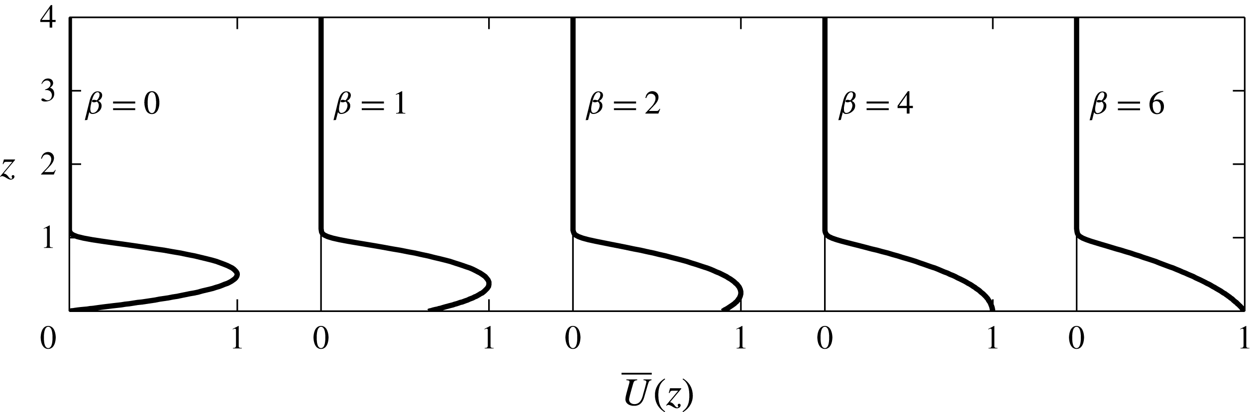
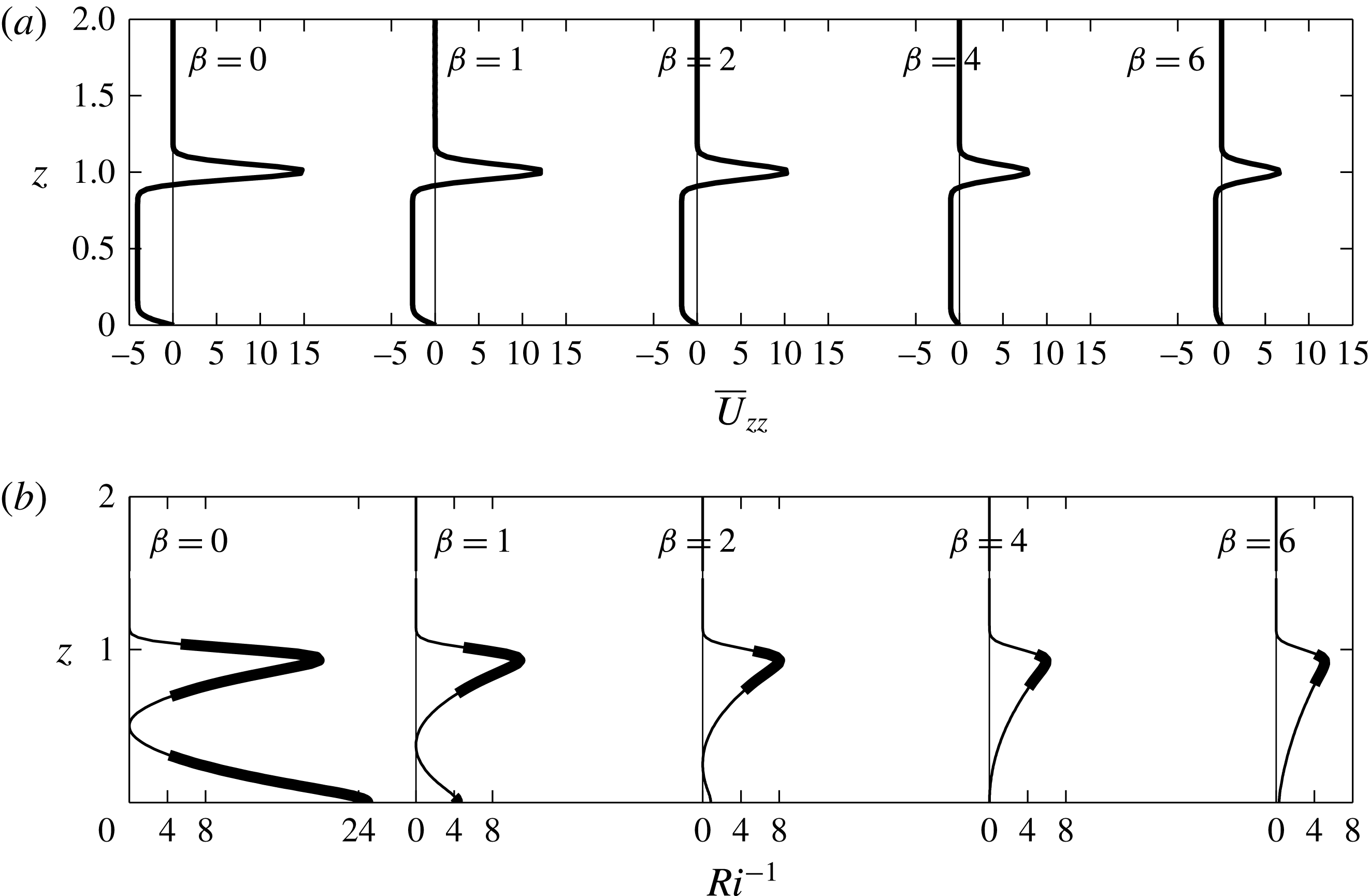
values, which corresponds to differences in speed at the lower free-slip boundary. Figures 3(a) and 3(b) display the corresponding vorticity gradient and inverse Richardson number curves for these flows. We shall return to the significance of these particular vorticity and Richardson number profiles in § 6.1.
The background velocity for the illustrative case of
 $\unicode[STIX]{x1D6FC}=0.5$
. As
 $\unicode[STIX]{x1D6FD}$
increases, the flow changes character from a pure parabolic jet towards a linearly sheared profile.

(a) Vorticity gradient and (b) corresponding inverse Richardson number (
 $Ri^{-1}$
) profile for the case
 $\unicode[STIX]{x1D6FC}=0.5$
. The thick lines in (b) correspond to subquarter
 $Ri$
regions. As the dynamically uncoupled layer is taken to be at rest, the vertical coordinate in the
 $Ri^{-1}$
plot has been truncated at
 $z=2$
, the top of the isolating layer.

It should be noted again that the values
 $\unicode[STIX]{x1D6FC}$
,
 $\unicode[STIX]{x1D6FD}$
and
 $Q$
conservation completely determine the profiles and define the stability problem. The dimensional expressions for velocity maximum, stratification and
 $Ri(z_{d})$
are derived below. Equation (2.4) gives
 $$\begin{eqnarray}U_{\unicode[STIX]{x1D6FF}_{i}}=\frac{\displaystyle \frac{2}{3}U_{0}}{\displaystyle \unicode[STIX]{x1D6FC}\left(\frac{2}{3}+\frac{\unicode[STIX]{x1D6FD}}{2}\right)}.\end{eqnarray}$$
Similarly, from (2.3), the stratification for a given value of
 $\unicode[STIX]{x1D6FC}$
is directly given by
 $$\begin{eqnarray}N_{\unicode[STIX]{x1D6FF}_{i}}=N_{0}/\sqrt{\unicode[STIX]{x1D6FC}}.\end{eqnarray}$$
Now, the optimal solution of Winters & Armi (Reference Winters and Armi2014) is characterized by an upstream parabolic jet with
 $$\begin{eqnarray}U_{0}=(3/2)N_{0}H/\unicode[STIX]{x03C0}.\end{eqnarray}$$
Using (2.2), (5.1)–(5.3), the Richardson number in the flowing layer can be written as
 $$\begin{eqnarray}Ri=\frac{N_{\unicode[STIX]{x1D6FF}_{i}}^{2}}{(\text{d}\bar{U}_{d}/\text{d}z_{d})^{2}}=\frac{\displaystyle \unicode[STIX]{x03C0}^{2}\unicode[STIX]{x1D6FC}\left(\frac{2}{3}+\frac{\unicode[STIX]{x1D6FD}}{2}\right)^{2}}{\displaystyle \left(\frac{4}{\unicode[STIX]{x1D6FC}}-\frac{8z_{d}}{\unicode[STIX]{x1D6FC}^{2}H}-\frac{\unicode[STIX]{x1D6FD}}{\unicode[STIX]{x1D6FC}}\right)^{2}}.\end{eqnarray}$$
The minimum value of (5.4) always occurs at
 $z_{d}=\unicode[STIX]{x1D6FC}H$
, or
 $z=1$
, i.e. at the upper edge of the flowing layer, and is given by
 $$\begin{eqnarray}Ri_{min}=\unicode[STIX]{x03C0}^{2}\unicode[STIX]{x1D6FC}^{3}\frac{\displaystyle \left(\frac{2}{3}+\frac{\unicode[STIX]{x1D6FD}}{2}\right)^{2}}{(4+\unicode[STIX]{x1D6FD})^{2}}.\end{eqnarray}$$
For each profile, we specify the wavenumber
 $k$
and solve the eigenvalue problem (3.7). We then sweep over a specified range of
 $0\leqslant k\leqslant 10$
to capture an order-1 aspect ratio K–H mode and extract the mode with the largest growth rate and the associated wavenumber
 $k_{max}$
and phase speed
 $c_{r}$
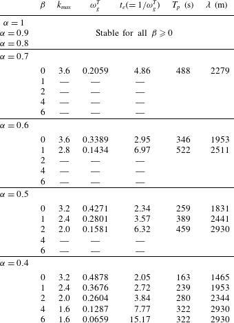
. Table 1 summarizes the results for particular values of
 $\unicode[STIX]{x1D6FC}$
and
 $\unicode[STIX]{x1D6FD}$
. We interpret the results in the context of hydraulically controlled stratified flow over topography, as in figure 1.
As the active layer crests the topography, the isolating layer increases in thickness, eventually triggering instability at a certain critical
 $\unicode[STIX]{x1D6FC}_{c}$
. We did not obtain any unstable modes for
 $\unicode[STIX]{x1D6FC}\geqslant 0.8$
, suggesting that
 $0.7\leqslant \unicode[STIX]{x1D6FC}_{c}\leqslant 0.8$
. The
 $e$
-folding time
 $t_{e}$
, which is the time it takes for the perturbation to increase by a factor of
 $e$
, is a useful characterization for comparison purposes. The
 $O(1)$
 $e$
-folding times for the unstable modes (table 1) are consistent with the nonlinear simulations of Scinocca & Peltier (Reference Scinocca and Peltier1989).
The dimensional values of the phase speed and wavelength of the most unstable mode are also presented in the last two columns of table 1 for the value of
 $H$
corresponding to the numerical study of Smith (Reference Smith1991). He reported the first significant unstable mode encountered downstream to have period and wavelength of 273 s and 2855 m respectively, which are also consistent with the ranges predicted by Scinocca & Peltier (Reference Scinocca and Peltier1989). While our values for these parameters are of the same order, the major differences are in the onset and growth rates of the unstable modes which we found to be over an order of magnitude larger.
Characteristics of the unstable mode in the two-parameter space of
 $\unicode[STIX]{x1D6FD}$
and
 $\unicode[STIX]{x1D6FC}$
. Here,
 $k_{max}$
is the wavenumber of maximum temporal growth rate
 $\unicode[STIX]{x1D714}_{g}^{T}=k_{max}c_{i}$
, where
 $c_{i}=\text{Im}(c)$
, and
 $t_{e}$
is the
 $e$
-folding time for the fastest growing mode, scaled by
 $h/U_{0}$
. A dash indicates that no unstable modes were found. The last two columns are the dimensional values of the period (
 $T_{p}$
) and wavelength (
 $\unicode[STIX]{x1D706}$
) of the unstable mode for the case
 $H\approx 1865$
as in the numerical experiments of Smith (Reference Smith1991).

For the upstream flow,
 $\unicode[STIX]{x1D6FC}=1$
and
 $\unicode[STIX]{x1D6FD}=0$
, which yields
 $Ri_{min}=\unicode[STIX]{x03C0}^{2}/36>1/4$
, which is stable by the Miles–Howard theorem. It should be noted that
 $Ri_{min}\sim \unicode[STIX]{x1D6FC}^{3}$
, so moving downstream, the large shear at the interface of the jet and the stagnant layer dominates the stabilizing effect of the stratification and increasing
 $\unicode[STIX]{x1D6FD}$
. This explains the persistence of unstable modes at low
 $\unicode[STIX]{x1D6FC}$
and relatively large
 $\unicode[STIX]{x1D6FD}$
seen in table 1.
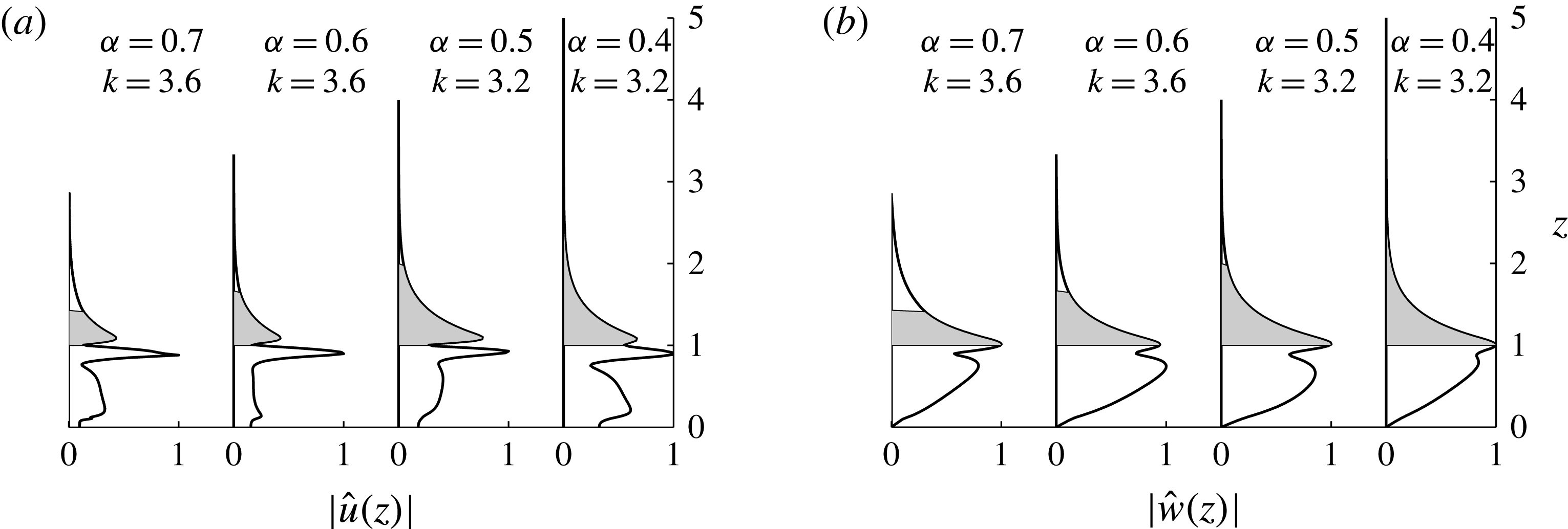
Normalized eigenfunctions (a)
 $|\hat{u} (z)|$
and (b)
 $|{\hat{w}}(z)|$
for
 $\unicode[STIX]{x1D6FD}=0$
. This represents the case where the bottom streamline is stationary, i.e. downslope flow evolves as a pure parabolic jet. The values
 $\unicode[STIX]{x1D6FC}=0.7,0.6,0.5$
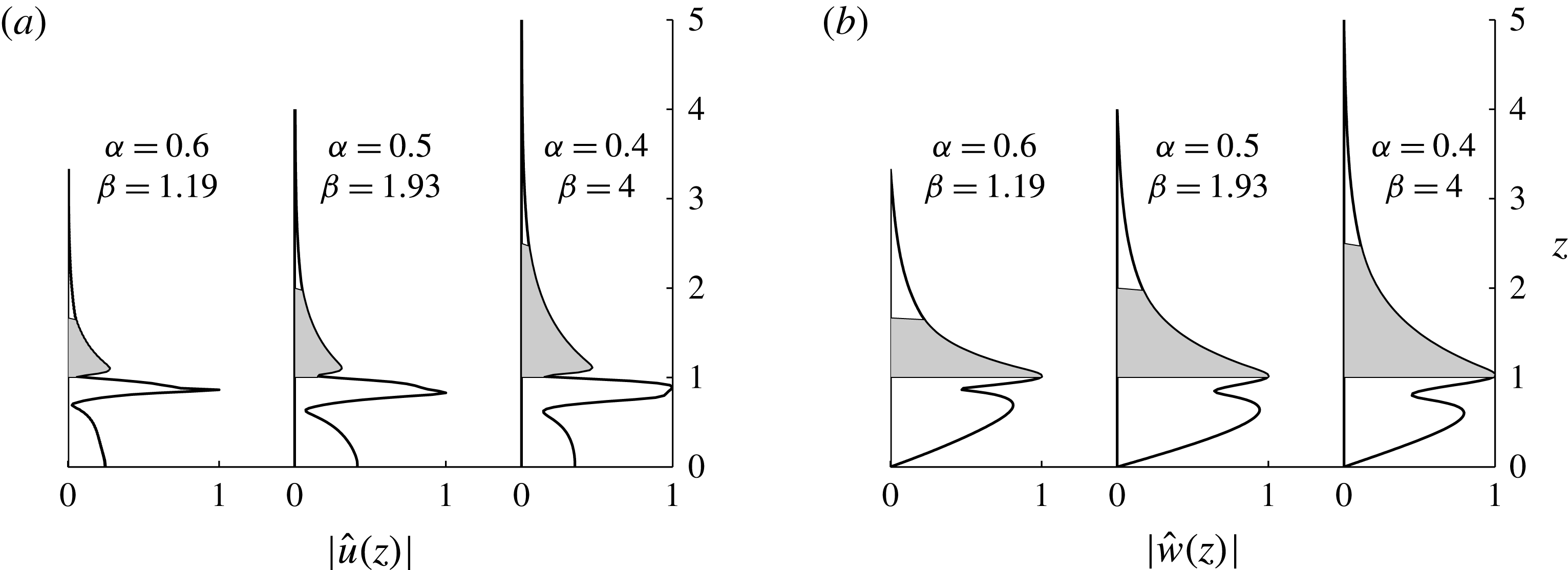
and 0.4 were all found to possess a growing mode. It should be noted that the lengths are non-dimensionalized using the height of the flowing layer at each location, so the isolating layer (shaded grey) lies between 1 and
 $1/\unicode[STIX]{x1D6FC}$
. Between
 $1/\unicode[STIX]{x1D6FC}$
and
 $2/\unicode[STIX]{x1D6FC}$
, the background flow is dynamically uncoupled and the eigenfunctions decay exponentially. The sharp behaviour of
 $|\hat{u} (z)|$
at
 $z=1$
is typical of a K–H mode at a shear interface.

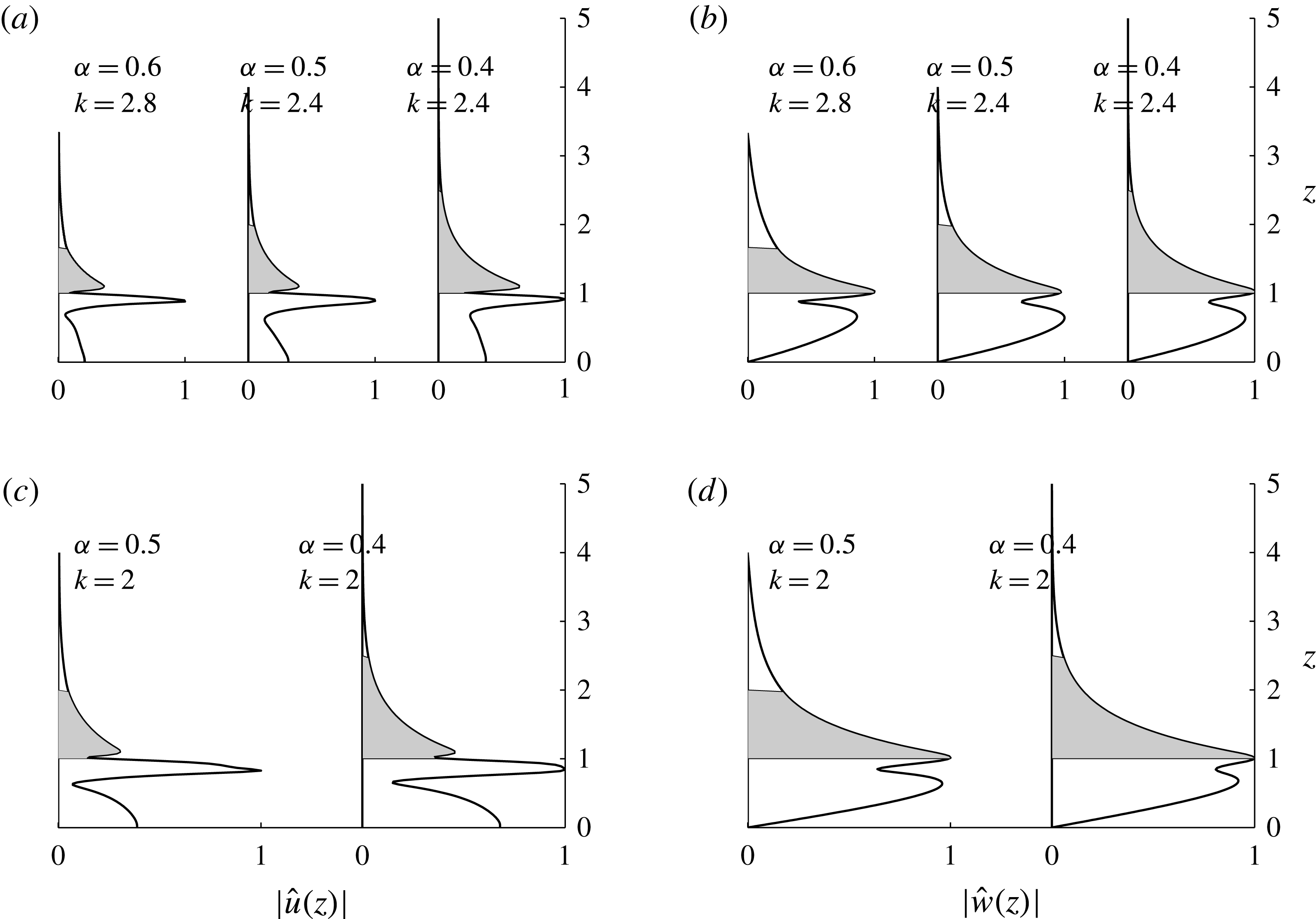
Normalized eigenfunctions (a), (c)
 $|\hat{u} (z)|$
and (b), (d)
 $|{\hat{w}}(z)|$
for
 $\unicode[STIX]{x1D6FD}=1,2$
, when the bottom streamline is not stationary, as for example in the case of a free-slip boundary. In this configuration, the velocity maximum for the base flow shifts downwards compared with the pure parabolic jet (see figure 2). For
 $\unicode[STIX]{x1D6FD}=1$
,
 $\unicode[STIX]{x1D6FC}=0.6,0.5$
and 0.4 are found to be unstable. When
 $\unicode[STIX]{x1D6FD}=2$
, the base profile is qualitatively similar to the case
 $\unicode[STIX]{x1D6FD}=1$
, but the larger bottom velocity appears to stabilize the flow for
 $\unicode[STIX]{x1D6FC}\geqslant 0.6$
.

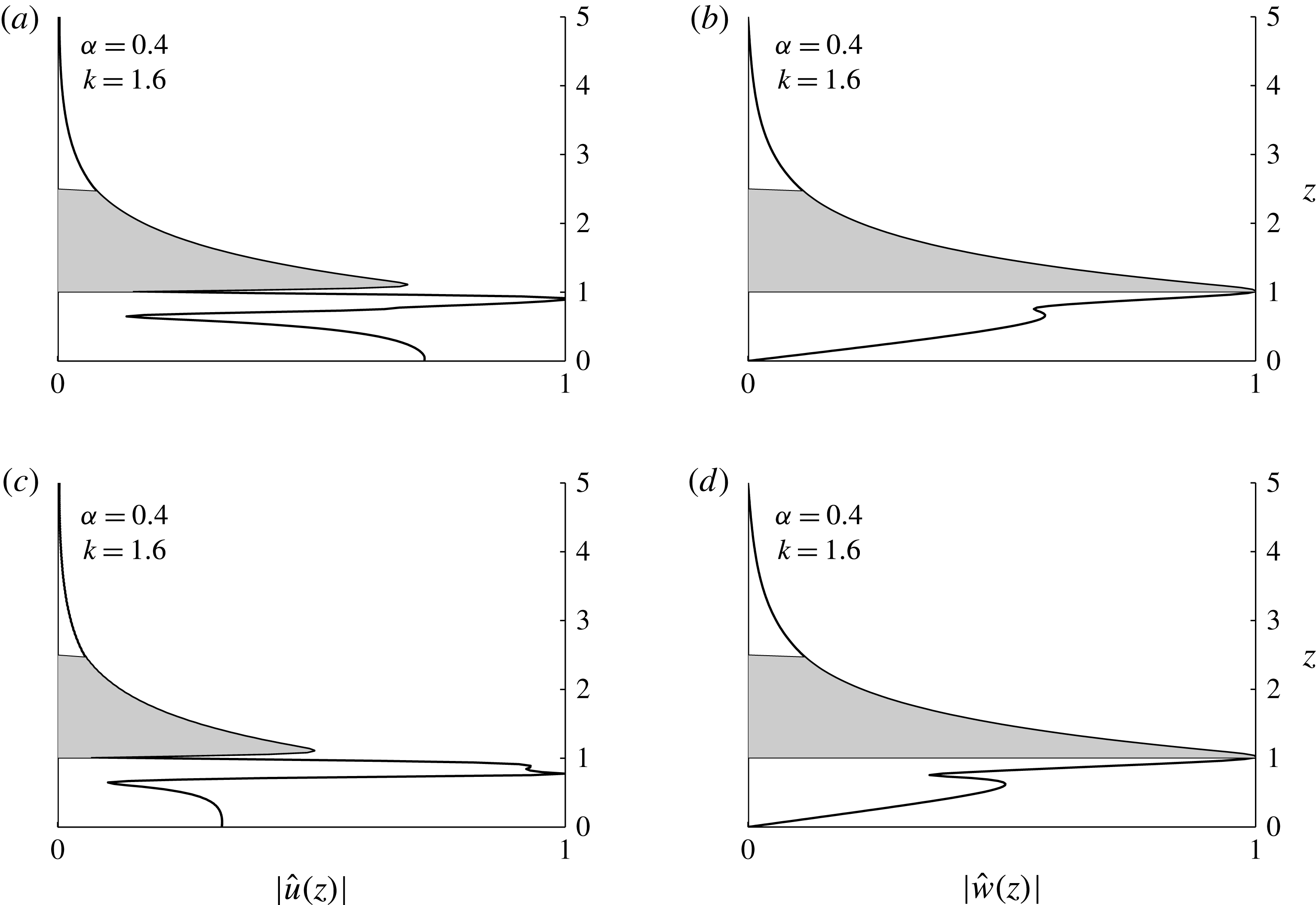
Normalized eigenfunctions (a),(c)
 $|\hat{u} (z)|$
and (b),(d)
 $|{\hat{w}}(z)|$
for
 $\unicode[STIX]{x1D6FD}=4,6$
. This represents the case where the linear component begins to dominate the profile. The value
 $\unicode[STIX]{x1D6FD}=4$
is the critical value where the velocity maximum coincides with the bottom streamline. For this configuration, only
 $\unicode[STIX]{x1D6FC}=0.4$
possesses sufficient shear to allow instability. At
 $\unicode[STIX]{x1D6FD}=6$
, the linear component clearly dominates the base profile (figure 2), but instability persists for
 $\unicode[STIX]{x1D6FC}=0.4$
.

Figures 4–6 display the normalized eigenfunctions for
 $|\hat{u} (z)|$
and
 $|{\hat{w}}(z)|$
. Their wavelengths (table 1) and shape identify them as unit-aspect-ratio overturning shear instabilities that nucleate at the upper edge of the flowing layer, where there is an abrupt jump in shear, as shown in figure 3.
6 Discussion
It should be recalled that Rayleigh’s theorem gives the presence of an inflection point as a necessary condition for instability in a homogeneous shear flow. The flows examined above are essentially sheared flows endowed with an inflection point, but in a stably stratified environment. Investigation of the stability of the corresponding homogeneous shear profile can help to clarify the nature of the instability in the stratified scenario. If shear were the driving mechanism of the instability, then we would expect stratification to have a stabilizing effect, modifying the unstable shear mode and reducing its growth rate.
Indeed, we found that, for every flow configuration for which an unstable mode was present, the growth rate for the same shear profile, but without a stable stratification, was larger. This identifies the unstable modes of table 1 as stratified analogues of inflectional Rayleigh modes, which, following the convention of Carpenter, Balmforth & Lawrence (Reference Carpenter, Balmforth and Lawrence2010), we refer to as Kelvin–Helmholtz modes. We further note that in the absence of stratification, the piecewise linear limit, corresponding to
 $\unicode[STIX]{x1D6FD}\rightarrow \infty$
, is stable for all values of
 $\unicode[STIX]{x1D6FC}$
. Our numerical results suggest that this also holds for piecewise continuous linear stratifications such as the ones under consideration here.
6.1 Physical interpretation of instability
The wave-interaction theory (see, e.g., Carpenter et al.
Reference Carpenter, Tedford, Heifetz and Lawrence2011) offers qualitative insight into the destabilizing mechanism at play. The key idea of the theory is that instability is possible whenever the flow configuration supports two or more waves whose directions of intrinsic propagation, relative to the local fluid velocity, are of opposite sign. Additionally, for a large class of stratified flows, Baines & Mitsudera (Reference Baines and Mitsudera1994) showed that an arbitrarily small region with
 $Ri<1/4$
, flanked on either side by regions where
 $Ri>1/4$
, is a sufficient condition for instability. Such a configuration effectively splits the flow into stable upper and lower waveguides, with no vertical wave propagation being possible in the central subquarter Richardson number region, a result effectively proved by Bell (Reference Bell1974). Two free modes in these separated waveguides can then interact to cause mutual changes in phase speed, inducing them to become stationary relative to one other, leading to mutual excitation and growth. This optimal ‘phase locked’ state is maintained over a range of wavenumbers through adjustments to the phase difference. On the other hand, if
 $Ri>1/4$
everywhere, internal wave modes are able to propagate vertically, eventually getting absorbed back into the mean flow at a critical layer in the central region, and the flow remains stable.
The
 $\bar{U}_{zz}$
profiles in figure 3 are seen to exhibit a large peak at
 $z=1$
, corresponding to the nearly discontinuous vorticity interface at the lower branch of the bifurcating streamline of figure 1. Below this, their values are constant, but reduced in strength and opposite in sign relative to the interface above. Thus, the intrinsic direction of propagation of vorticity waves in each of these regions is opposite, satisfying one of the necessary conditions of the wave-interaction theory.
To see in more detail how these particular vorticity profiles can lead to instability, we consider again the corresponding unstratified flow. It should be noted that, unlike the prototypical examples of piecewise linear and continuous vorticity distributions for which the wave-interaction mechanism has been invoked to understand shear instability (e.g. Carpenter et al.
Reference Carpenter, Tedford, Heifetz and Lawrence2011), in these flows, the vorticity profiles exhibit only one (and not two) distinct extremum. Thus, the view of the instability as an interaction between two interfacial (or smeared) vorticity waves breaks down, and it is necessary to include the continuous spectrum in the analysis. When the flow is quasi-jet-like, with
 $\unicode[STIX]{x1D6FD}\sim O(1)$
, the unstable inflectional mode may be regarded as arising due to the interaction between the interfacial rightward propagating vorticity wave riding on the shear interface at
 $z=1$
and a wave belonging to the continuous spectrum supported in the region of constant vorticity between
 $z=0$
and
 $z=1$
. The abrupt change in the
 $\hat{u} (z)$
eigenfunction near
 $z=1$
in figures 4–6 is typical of a vorticity wave propagating at a shear jump, and further bolsters this view of the instability mechanism. When a stable stratification is added, the vorticity modes are modified by the buoyancy, leading to weakened interaction and, consequently, reduced growth rates.
Inspection of figure 3 shows that the Baines & Mitsudera (Reference Baines and Mitsudera1994) condition on the Richardson number profiles is also met for these flows. The thin lines denote separate stable waveguides where
 $Ri>1/4$
. These are separated by a region (thick line) where
 $Ri<1/4$
and internal wave propagation cannot occur. Approximating
 $z=1$
as a discontinuous shear interface, the speed of the rightward propagating vorticity wave here is given by, to first order,
 $$\begin{eqnarray}c_{1}\approx \frac{\bar{U}_{z}|_{z=1^{-}}}{2k}.\end{eqnarray}$$
The flow configurations in the stable lower waveguide yield a discrete spectrum of internal wave modes modified by the shear in addition to a continuous spectrum whose eigenvalues lie in the range of
 $\bar{U}$
. In the absence of stratification, the same shear profiles support only a continuous spectrum whose properties, however, differ from those of the continuous spectrum for the corresponding stratified flow. Further, Howard’s (Reference Howard1961) semicircle theorem constrains the real phase speed of an unstable mode for this flow to lie within the range of fluid velocity. Therefore, given the lack of a clear shear or density interface in the lower waveguide, it seems likely that for both the stratified and the unstratified flow, it is the interaction between the interfacial vorticity wave and a wave in the continuous spectrum that gives rise to instability.
To test this hypothesis, we added a small amount of viscosity and diffusivity and solved the sixth-order Taylor–Goldstein equation for the flow configurations in the lower waveguide. Free slip and an exponential decay condition for
 ${\hat{w}}(z)$
at the upper boundary filter the unstable Tollmien–Schlichting waves from the computation. The wave modes thus obtained are essentially similar to what we would find for the inviscid flow – vorticity waves modified by buoyancy and vice versa – with the difference being that the singularity of the second-order Taylor–Goldstein equation is avoided and, consequently, the continuous spectrum collapses onto a discrete set of decaying modes. For the case
 $\unicode[STIX]{x1D6FC}=0.5,\unicode[STIX]{x1D6FD}=2$
, we found that at
 $k=5$
, there are two modes with speeds
 ${\approx}0.26$
, which is roughly the same value that was found on applying (6.1) and which also matches the real part of the eigenvalue of the unstable mode that was found by solving the Taylor–Goldstein equation for the complete profile in figure 2. Thus, we have all the necessary elements for the wave-interaction theory to be invoked; instability persists over a range of wavenumbers by mutual interaction, leading to phase and amplitude locking.
For larger values of
 $\unicode[STIX]{x1D6FD}$
, the shear gradient below
 $z=1$
is too weak to induce a mutual growth with the vorticity wave riding aloft at
 $z=1$
. In the piecewise linear limit
 $\unicode[STIX]{x1D6FD}\rightarrow \infty$
, there is exactly one vorticity interface at
 $z=1$
; no fundamental unstable shear mode is present, and thus the addition of a linear stratification apparently has no effect on the stability of the flow. As a corollary, we surmise that no unstable wave interactions are possible in a piecewise linear stably stratified environment where there are no density jumps and where the shear is uniform on either side of a single vorticity interface.
In light of this explanation, we speculate that the late onset of instability and small growth rates of Smith (Reference Smith1991) result from truncating the base flow at the upper edge of the active layer. This excludes a vorticity wave at the upper boundary and, consequently, no destabilizing wave interactions are possible in the flow. We note, however, that, despite the lack of an inflection point in the profiles, the exponential decay implied by their upper boundary condition does not completely exclude the possibility of instability and, indeed, the weak growth rates predicted might well be a consequence of this. In contrast, we have included both the isolating layer and the dynamically uncoupled flow in our analysis. This, besides imposing precise no-normal-flow conditions at both boundaries, also furnishes an inflection point to the velocity profile – a necessary condition for stability of unstratified shear flow – as well as a region of weak stratification close to the inflection point (giving
 $Ri<1/4$
), which may trigger an unstable shear mode via the wave-interaction mechanism described above.
6.2 Spatial instability and the Winters & Armi (Reference Winters and Armi2014) downslope flow
We mentioned in § 2 that the Winters & Armi (Reference Winters and Armi2014) solution for optimally controlled stratified flow over topography is a special case where
 $\unicode[STIX]{x1D6FC}$
and
 $\unicode[STIX]{x1D6FD}$
are not independent, but uniquely related. We once again refer to figure 10 of Winters & Armi (Reference Winters and Armi2014) and note that the accelerating bottom streamline characteristic of this solution corresponds, in our present formulation, to increasing
 $\unicode[STIX]{x1D6FD}$
downstream. For different values of
 $\unicode[STIX]{x1D6FC}$
, values of
 $\unicode[STIX]{x1D6FD}$
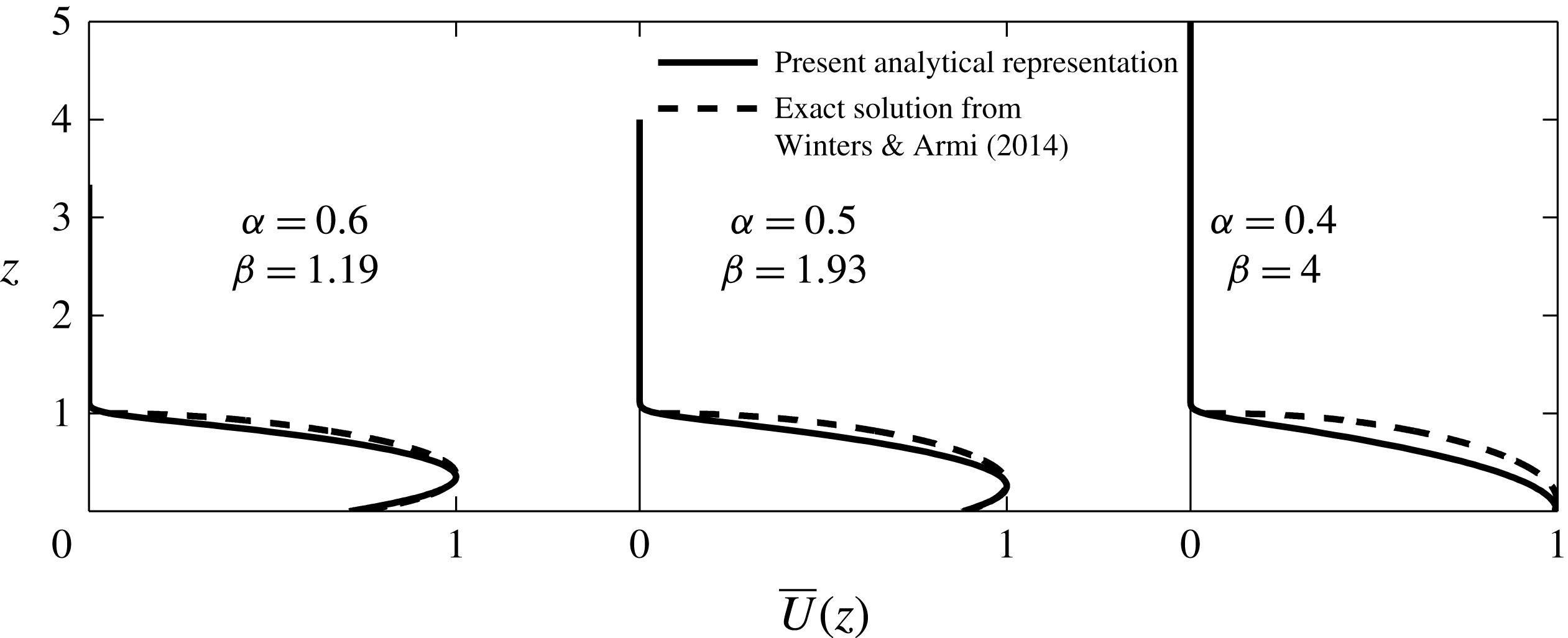
and the fit they produce to the actual solutions of Winters & Armi (Reference Winters and Armi2014) are shown in figure 7. Clearly, the parameter pairs
 $(\unicode[STIX]{x1D6FC},\unicode[STIX]{x1D6FD})$
are quite close to the cases studied in § 5, and we may expect a stability analysis to yield similar results. Inspection of the eigenfunctions of the fastest growing modes (figure 8) and their growth characteristics (table 2) confirms this to be the case.
The Winters & Armi (Reference Winters and Armi2014) background velocity profiles at different downstream locations for the optimally controlled stratified downslope flow. The dashed lines are the exact solutions and the solid lines are the representations of these solutions using
 $\unicode[STIX]{x1D6FD}$
and
 $Q$
conservation.

Normalized eigenfunctions (a)
 $|\hat{u} (z)|$
and (b)
 $|{\hat{w}}(z)|$
for the profiles representative of the solutions of Winters & Armi (Reference Winters and Armi2014).

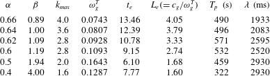
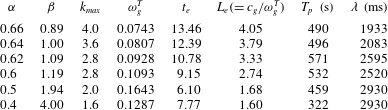
Characteristics of the unstable mode for the flow profiles representative of the exact solutions of Winters & Armi (Reference Winters and Armi2014). Here,
 $L_{e}$
is the
 $e$
-folding length for the fastest growing spatial mode, scaled by
 $h$
(see § 6.2 for more details) and
 $c_{g}$
is the group velocity of the mode given by
 $c_{g}=\unicode[STIX]{x2202}\unicode[STIX]{x1D714}_{r}/\unicode[STIX]{x2202}k$
, where
 $\unicode[STIX]{x1D714}_{r}=\text{Re}(kc)$
. Refer to table 1 for more details on notation.
Our discussion so far has been restricted to the temporally growing modes for which the underlying assumption is that the perturbations to the base flow may be distinguished by their horizontal wavenumbers. However, disturbances could, in principle, also assume the form of a pulse or a localized source vibrating at a fixed frequency, in which case spatially growing modes may be triggered. In the case of the former, growing disturbances are either convected away from the source (convective instability) or grow in situ (absolute instability), destroying the base flow itself for large time. The case of a local periodic forcing constitutes the so-called signalling problem and again may lead to either spatially amplified sinusoids (convective mode) or absolute instability. Huerre et al. (Reference Huerre, Batchelor, Moffatt and Worster2000) provides a general discussion of these and other aspects of the spatial instability problem, including an elegant technique for determining whether a given flow is absolutely unstable or not.
Downslope flows in nature are subject to a wide range of perturbations and are thus potentially susceptible to both temporal and spatial modes of instability. It can thus be difficult in practice to precisely establish whether an observed instability mode is a purely spatial one or some combination of temporal and spatial modes. However, guided by consideration of the observed growing modes in Farmer & Armi (Reference Farmer and Armi1999) and Winters (Reference Winters2016), we rule out the possibility of absolute growth at any downstream location. Further, for the sake of simplicity, we stay within the framework of the spatial signalling problem for the reminder of this discussion.
It should be recalled that the optimal horizontally uniform upstream flow configuration of Winters & Armi (Reference Winters and Armi2014) is stable at the blocking location
 $x_{b}$
, with
 $Ri_{min}$
being slightly greater than 1/4. Thereafter, as the upper streamline bifurcates and the flowing layer accelerates,
 $Ri_{min}$
eventually drops down below
 $1/4$
, allowing for the possibility of unstable modes.
As shown in table 2, for the optimally controlled solutions of Winters & Armi (Reference Winters and Armi2014), we found that the flow first exhibits temporal instability where
 $\unicode[STIX]{x1D6FC}\approx 0.67$
. Upstream of this location, the growth rates found were too small to pass the spurious mode detection criterion of § 4, and downstream of this point, the growth rate appears to increase rapidly, growing to order
 $O(10^{-1})$
at
 $\unicode[STIX]{x1D6FC}_{c}\approx 0.6$
. The increasing shear at
 $z=1$
downstream appears to be offset by the weakening shear at the bottom streamline of the flowing layer along which the flow accelerates as it ascends and plunges down the obstacle, and so the growth rate and
 $e$
-folding scales continue to be
 ${\sim}O(10^{-1})$
and
 ${\sim}O(1)$
at further downstream locations as well.
6.2.1 The spatial signalling problem in the framework of Gaster (Reference Gaster1962)
It is perhaps instructive to picture a curve of marginal stability (CMS),
 $$\begin{eqnarray}\unicode[STIX]{x1D714}=f(k,\unicode[STIX]{x1D6FC},\unicode[STIX]{x1D6FD}),\end{eqnarray}$$
for this problem, with
 $\unicode[STIX]{x1D714}$
being real valued on one side of the curve and complex on the other. For the upstream flow,
 $\unicode[STIX]{x1D6FC}=1,\unicode[STIX]{x1D6FD}=0$
,
 $\unicode[STIX]{x1D714}$
is real valued for all
 $k$
. The first location where an unambiguously distinguishable unstable mode is encountered is for
 $\unicode[STIX]{x1D6FC}\approx 0.66$
. It may thus be reasonably surmised that the point
 $(k,\unicode[STIX]{x1D6FC},\unicode[STIX]{x1D6FD})=(4,0.66,0.89)$
in parameter space is close to the CMS for the flow. This in turn allows us to appeal to the framework of Gaster (Reference Gaster1962) in which, near the CMS and for a given wavenumber, the growth rate of an unstable spatial mode can be estimated to first order from the corresponding temporal mode through the formula
 $$\begin{eqnarray}k_{g}^{s}=-\unicode[STIX]{x1D714}_{g}^{T}/c_{g},\end{eqnarray}$$
where
 $$\begin{eqnarray}c_{g}=\frac{\unicode[STIX]{x2202}\unicode[STIX]{x1D714}_{r}}{\unicode[STIX]{x2202}k}=\frac{\unicode[STIX]{x2202}\text{Re}(kc_{r})}{\unicode[STIX]{x2202}k}\end{eqnarray}$$
is the group velocity of the temporal instability mode, which we compute numerically. Although, strictly speaking, we have only argued that the first upstream unstable mode is close to the CMS, we use (6.3) to approximate the spatial growth rate at locations further downstream as well. In reality, for parameter values that are well away from the CMS, it is probably necessary to consider the dispersion relation in the complex
 $(\unicode[STIX]{x1D714},k)$
plane to obtain more accurate results for the spatial problem. We shall demonstrate below that ultimately it is the most upstream unstable mode, close to the CMS, that dominates the spatial growth of instability in streamwise slowly varying controlled downslope flows.
In table 2, we found the group velocity to be non-zero and positive in all cases, establishing them as convective rather than absolute modes of instability. Thus, we can define an
 $e$
-folding length, analogous to the time scale defined in § 5,
 $L_{e}=c_{g}/\unicode[STIX]{x1D714}_{g}^{T}$
. This is the distance by which a growing mode propagates downstream as it undergoes amplification by a factor of e. In field measurements and numerical simulations, we detect only the finite-amplitude manifestation of an instability, which typically occurs at a downstream position that is of the order of a few
 $e$
-folding lengths.
6.2.2 Evolution to finite amplitude
We reiterate that the flow configurations examined here are approximations to analytical solutions in the purely hydrostatic limit, i.e. when the horizontal length scale is infinite. In this limit, the parallel flow assumption holds everywhere, and so the very first unstable mode will have sufficient downstream distance to grow and undergo amplification to finite amplitude. In the process, it irreversibly changes the flow configuration further downstream through nonlinear interactions with the base flow. However, we have not discounted the possibility that when the topography is steep enough, with horizontal length scale
 $L_{x}$
, the initial weakly unstable spatial modes will have insufficient distance to grow before the background flow profile changes significantly. Then, these weakly growing modes effectively act as perturbations to the flow further downstream, potentially exciting a stronger unstable mode at some location. In such a case, we would have to examine the growth rates and
 $e$
-folding length scales of the growing modes at various downstream locations, and the first mode that satisfies
 $L_{e}\ll L_{x}$
would be the one that would eventually dominate the other modes and lead the transition to nonlinearity.
To investigate this in more detail, suppose that the horizontal length scale for the flow is
 $L_{x}$
. One plausible definition of
 $L_{x}\gg H$
is the downstream distance over which the thickness of the flowing layer changes by 10 %. Now, for the hydrostatic approximation to hold, we require
 $L_{x}/H\sim O(10)$
. Since we are interested in the lower limit, suppose that
 $L_{x}/H\approx 10$
. Now, recalling that in our computations, the lengths are non-dimensionalized by
 $h$
, the local flowing layer thickness, from table 2, the growing mode at
 $\unicode[STIX]{x1D6FC}=0.66$
has
 $L_{e}=4.05h=4.05\unicode[STIX]{x1D6FC}H=2.68H$
. Therefore, an initial disturbance at this location will have sufficient downstream distance to grow to
 $\exp 10/2.48\approx 42$
times its initial magnitude before the background profile changes significantly. This is more than an order of magnitude amplification and hence will be manifested physically in observations and numerical simulations at
 $h/H\approx 0.56$
before nonlinearities eventually modify the character of the background flow itself further downstream. Thus, even at the boundary of the hydrostatic regime when
 $L_{x}/H\approx 10$
, it appears that the very first spatial mode excited that has
 $O(1)$
 $e$
-folding length scale is the one that dominates the instability process in these flows.
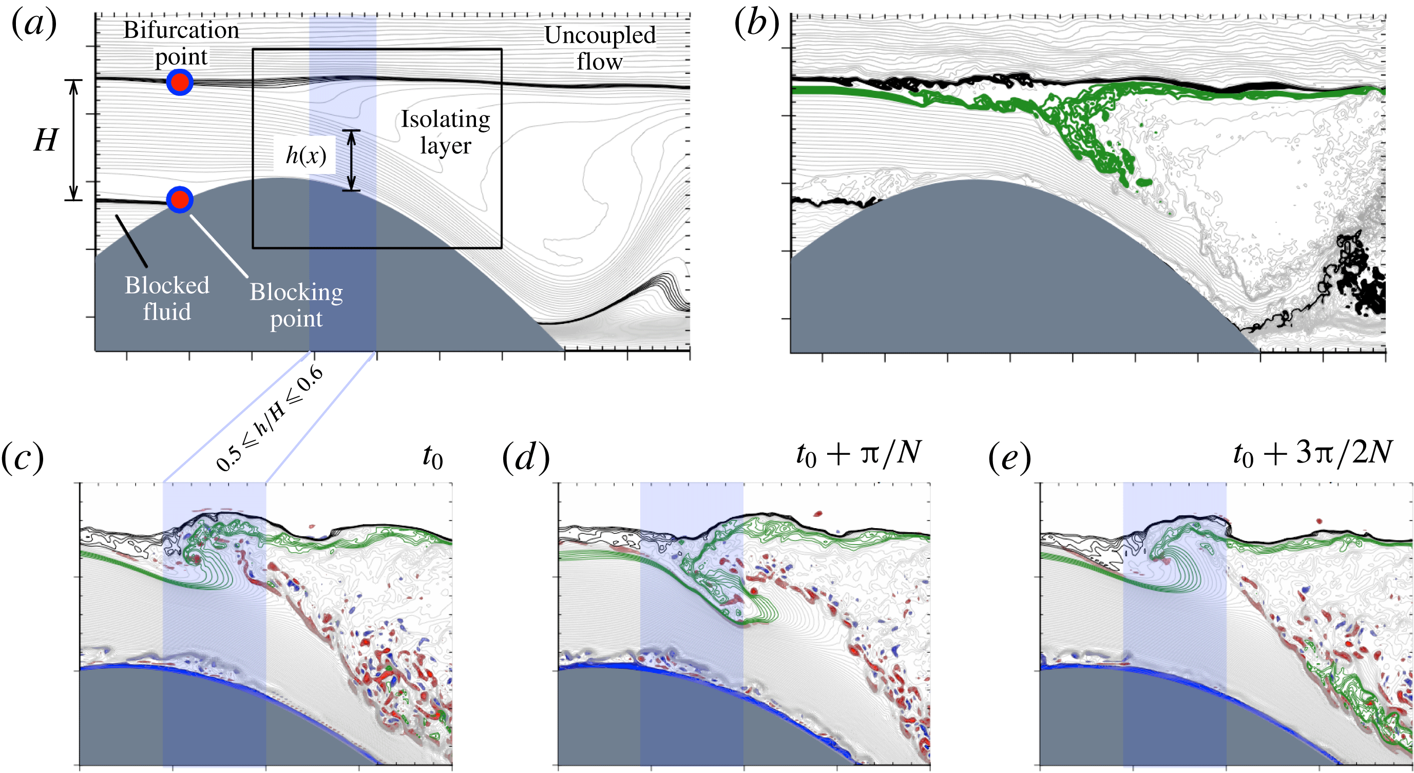
(Winters Reference Winters2016) Isopycnals and vorticity from a statistically steady nonlinear simulation of stratified flow over a smooth topography matching the optimal upstream solution of Winters & Armi (Reference Winters and Armi2014). The value of
 $L_{x}/H$
for this flow is
 ${\sim}O(10)$
, i.e. it is at the boundary of the hydrostatic regime. (a) The time and cross-stream averaged flow that exhibits the essential features of the flow and (b) an instantaneous snapshot of the flow. (c–e) Three snapshots of the flow spaced approximately half a buoyancy period apart. Shear instability is observed at the upper edge of the flowing layer, and finite-amplitude billow structures are first perceived within the shaded region
 $0.5\leqslant h/H\leqslant 0.6$
, where repeated overturning and plunging of the lower isopycnals (coloured green for visualization purposes) is also visible. The red and blue colours indicate positive and negative vorticity extrema respectively.

This result is also in agreement with figure 12 of Farmer & Armi (Reference Farmer and Armi1999), where, for a flow with
 $L_{x}/H\sim O(10)$
, the centre of the first finite-amplitude vortex core in the lee, corresponding to the first physically observed overturning shear instability, is seen to occur at roughly
 $X=50$
m, giving
 $\unicode[STIX]{x1D6FC}\approx 0.55$
. Further, recent work by Winters (Reference Winters2016) also seems to corroborate this. Figure 9 shows the isopycnals from a statistically steady 3D simulation (see the supplementary movie available at https://doi.org/10.1017/jfm.2016.683) of stratified flow over topography matching the optimal upstream solution of Winters & Armi (Reference Winters and Armi2014), again for a flow with
 $L_{x}/H\sim O(10)$
. The simulation uses the same downstream condition as in figure 4 of Winters (Reference Winters2016). It is noted in his paper that the downstream condition has no effect on the flow over the sill in the region where this particular instability is observed. It primarily affects the point of downstream flow separation and the strength of the internal hydraulic jump. For our purposes, a quasisteady state was attained on time and spatial averaging over 6.25 buoyancy periods. Winters (Reference Winters2016) gives further details on the modelling and on how the flow solutions are affected by the downstream condition.
As anticipated by the analytical solutions of Winters & Armi (Reference Winters and Armi2014), upstream blocking, streamline bifurcation and formation of an isolating layer are clearly observed in this simulation. Further, the flow exhibits instability along the upper edge of the flowing layer, with finite-amplitude features manifested within the shaded region
 $0.5\leqslant h/H\leqslant 0.6$
. The location of the repeated overturns is also consistent with our prediction above that the finite-amplitude billows seen at
 $h/H\approx 0.56$
are in fact the physical manifestation of the spatially growing mode triggered further upstream at
 $h/H\approx 0.66$
.
6.3 Applicability to other flow regimes
A final note is that, while the stability analysis described here is formally valid only for the asymptotic regime of a tall mountain barrier with slow flow and/or strong stratification, even in situations where there is no blocking and upstream influence, the dynamics of the downstream flow evolution – namely an accelerating thinning jet with a stagnant mixed layer aloft – is largely identical, as can be seen, for example, in the work of Lilly (Reference Lilly1978) and Scinocca & Peltier (Reference Scinocca and Peltier1989). We therefore speculate that this overall view of the stability problem carries over to other regimes, including those with an initial uniform upstream flow profile.
7 Conclusion
We have analysed the linear stability of stratified flow profiles that are typically encountered in the downslope region of topographical features in the ocean and atmosphere. By considering idealized representations of jet-like profiles that emerge from a theoretical hydraulic view of the problem as in Winters & Armi (Reference Winters and Armi2014), we obtain growth rates that are between one and two orders of magnitude larger than those seen in the linear stability analysis of Peltier & Scinocca (Reference Peltier and Scinocca1990) and Smith (Reference Smith1991), and are consistent with the results of the nonlinear numerical simulations of Scinocca & Peltier (Reference Scinocca and Peltier1989).
We believe that it is the formal inclusion of a stagnant homogeneous isolating layer in the stability analysis that is responsible for such a dramatic improvement in the prediction of linear stability theory. The presence of a deep isolating layer above a strongly sheared jet-like flowing layer creates conditions that are favourable for the nucleation of shear instabilities. The sharp gradients in the horizontal velocity eigenfunction at
 $z=1$
and the fact that larger growth rates were obtained on solving the Rayleigh equation for the corresponding unstratified velocity profiles unambiguously identify them as K–H shear modes. The wave-interaction interpretation of shear flow instability appears to offer a satisfactory explanation for the observed instabilities. Further, an analysis of the spatial stability problem in the framework of small deviations from the CMS is shown to yield
 $O(1)$
 $e$
-folding length scales. These signal transition to nonlinearity at downstream distances that are consistent with those reported in observations and numerical simulations of downslope flows.
Acknowledgements
We wish to thank the reviewers for their very constructive and helpful comments. This work was supported by the National Science Foundation, grant AGS-1540585. XSEDE computing resources were made available under grant TG-OCE120004.
Supplementary movie
A supplementary movie is available at https://doi.org/10.1017/jfm.2016.683.