


1. Introduction
1.1. Motivation and background
The physics of inertial particles suspended in a turbulent boundary layer are of relevance in a number of settings, including the aeolian transport of pollen, snow, dust or sand in the atmospheric boundary layer, transport of sediment in rivers and various industrial applications. As such, they have been subject of intense studies since the seminal work of Rouse (Reference Rouse1937) and Prandtl (Reference Prandtl1952). Our understanding of the particle spatial distribution, transport and interaction with wall turbulence has greatly improved in the last decades thanks to advances in non-intrusive laser diagnostics (e.g. Kaftori, Hetsroni & Banerjee Reference Kaftori, Hetsroni and Banerjee1995a,Reference Kaftori, Hetsroni and Banerjeeb; Tanière, Oesterlé & Monnier Reference Tanière, Oesterlé and Monnier1997; Kiger & Pan Reference Kiger and Pan2002; Kussin & Sommerfeld Reference Kussin and Sommerfeld2002; Righetti & Romano Reference Righetti and Romano2004; van Hout Reference van Hout2011; Li et al. Reference Li, Wang, Liu, Chen and Zheng2012; Fong, Amili & Coletti Reference Fong, Amili and Coletti2019), and computational fluid dynamics (e.g. Marchioli & Soldati Reference Marchioli and Soldati2002; Zhao, Andersson & Gillissen Reference Zhao, Andersson and Gillissen2010; Sardina et al. Reference Sardina, Schlatter, Brandt, Picano and Casciola2012; Bernardini Reference Bernardini2014; Richter & Sullivan Reference Richter and Sullivan2014; Lee & Lee Reference Lee and Lee2015; Richter & Chamecki Reference Richter and Chamecki2018). By necessity, computational studies have adopted simplifying assumptions, e.g. neglecting gravitational settling and representing the particles as material points experiencing Stokesian drag. Also, most previous studies (both numerical and experimental) have considered relatively low friction Reynolds numbers,  $Re_\tau = \delta U_\tau /\nu = \textit{O}(10^2)$, where
 $\delta$ is the boundary-layer thickness (or channel half-height),
 $U_\tau$ is the friction velocity and
 $\nu$ is the kinematic viscosity.
We focus on the case in which gravity (perpendicular to the wall) has a key role and the Reynolds number is large, as relevant to dust/sand transport in the atmospheric boundary layer. This has typical Reynolds numbers 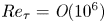 $Re_\tau = \textit{O}(10^6)$ and, for a typical ratio of friction velocity to free-stream velocity
 $U_\tau /U_\infty = \textit{O}(10^{-1})$, the separation between the largest and smallest time scales is
 $Re_\tau U_\tau /U_\infty = \textit{O}(10^5)$. That has far-reaching consequences for particle–turbulence interaction. The latter is typically characterized by the Stokes number, the ratio between the particle response time (
 $\tau _p$) and a relevant fluid time scale (
 $\tau _f$),
 $St=\tau _p/\tau _f$. When
 $St \gg 1$, particles are expected to be quasi-ballistic, while for
 $St \ll 1$ they are expected to faithfully follow the fluid. The vast time-scale separation of high-
 $Re$ wall-bounded flows implies that particles that act as tracers in the outer region of the boundary layer may be ballistic in the near-wall region.
In this study we carry out a laboratory investigation of the transport of small size-selected solid particles in air turbulent boundary layers at relatively high friction Reynolds number ( $Re_\tau = \textit{O}(10^4)$), in a regime close to equilibrium and for which the particles are fully suspended (i.e. no wall deposition). Using two-phase particle imaging, we simultaneously measure the motion of both the particles and the air. This is leveraged to gain insight in the mechanisms that determine the particle concentration and the streamwise velocity of the particles at various distances from the wall. The paper is organized as follows: in § 1.2 we review the classic theory behind the well-known power-law profiles of particle concentration and flux, to which we shall compare our data; in § 2 we describe the wind tunnel experiments, the imaging approach and the parameter space; the results are presented in § 3, in particular concerning particle concentration (§ 3.1), slip velocity (§ 3.2) and topology of the flow sampled by the particles (§ 3.3); in § 4 we summarize the findings and draw the main conclusions.
1.2. The theory of Rouse and Prandtl
We consider the time-averaged wall-normal profiles of concentration  $C$, streamwise velocity
 $U_p$ and flux
 $CU_p$ of particles suspended in a turbulent boundary layer. The streamwise particle velocity is often assumed equal to the fluid velocity (see, e.g. Chou & Fringer Reference Chou and Fringer2008; Lehning et al. Reference Lehning, Löwe, Ryser and Raderschall2008; Chamecki & Meneveau Reference Chamecki and Meneveau2011), and this assumption will be directly tested against our data in § 3. The fluid velocity has a wall-normal profile well described by the logarithmic law valid between
 $y^+>30$ and
 $y/\delta < 0.2$ (Coles Reference Coles1956)
 \begin{equation} U_f^+ = \frac{1}{\kappa} \log\left(y^+\right) + B, \end{equation}
where  $y$ is the distance from the wall,
 $\kappa$ is the von Kármán constant,
 $B \approx 5.2$ and the superscript ‘
 $+$’ refers to units normalized by the viscous scales of the flow. An alternative description is the power-law profile (Barenblatt, Chorin & Prostokishin Reference Barenblatt, Chorin and Prostokishin2000)
 \begin{equation} \frac{U_f}{U_r} = \left(\frac{y}{y_r}\right)^\alpha, \end{equation}
where  $U_r$ is the velocity at arbitrary reference height
 $y_r$, and
 $\alpha$ is a constant that for the Reynolds numbers in the present study is approximately equal to
 $1/6$ (Barenblatt et al. Reference Barenblatt, Chorin and Prostokishin2000). While it is established that the logarithmic description is superior in accuracy (Marusic et al. Reference Marusic, McKeon, Monkewitz, Nagib, Smits and Sreenivasan2010), here one may use the power-law approximation for mathematical simplicity, as the concentration profile is also commonly described by a power law.
We now briefly derive the classic mean concentration profile as predicted by Rouse (Reference Rouse1937) and Prandtl (Reference Prandtl1952), which we will refer to as the Rouse–Prandtl model. This is still the de facto standard in environmental transport (Boudreau & Hill Reference Boudreau and Hill2020). Starting from the continuity equation
 \begin{equation} \frac{\partial C}{\partial t} + \boldsymbol{\nabla} \boldsymbol{\cdot} \left(C \boldsymbol{U}_{\boldsymbol{p}}\right) = 0, \end{equation}
where  $\boldsymbol {U}_{\boldsymbol {p}}$ is the particle-velocity vector. Taking the time average, assuming steady state and expanding the vector product
 \begin{equation} \frac{\partial \overline{C U_p}}{\partial x} + \frac{\partial \overline{C V_p}}{\partial y} + \frac{\partial \overline{C W_p}}{\partial z} = 0, \end{equation}
where  $U_p$,
 $V_p$ and
 $W_p$ are the streamwise (
 $x$), wall-normal (
 $y$) and spanwise (
 $z$) components of the particle velocity. Here and in the following we use overbar and lowercase to denote time-averaged and fluctuating quantities, respectively. Re-arranging and integrating in the wall-normal direction
 \begin{equation} \overline{CV_p} = -\int \frac{\partial \overline{CU_p}}{\partial x}\,\mathrm{d}y - \int \frac{\partial \overline{CW_p}}{\partial z} \,\mathrm{d}y + \phi_0, \end{equation}
where  $\phi _0$ is an integration constant. Reynolds decomposition of the left-hand side and lumping together the three terms on the right-hand side yields
 \begin{equation} \bar{C} \,\overline{V_p} + \overline{cv_p} = \phi, \end{equation}
where  $\phi$ is the net vertical flux, which equals the sum of the advective flux (
 $\bar {C} \, \overline {V_p}$) and the diffusive flux (
 $\overline {cv_p}$). The vertical flux is in general a function of the wall-normal location, but if one assumes a two-dimensional flow (
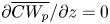 $\partial \overline {CW_p}/\partial z = 0$) and a fully developed concentration profile (
 $\partial \overline {CU_p}/\partial x = 0$), the net vertical flux is constant and equal to
 $\phi _0$. We consider quantities averaged in the streamwise and spanwise directions, thus (1.6) has a spatial dependence on
 $y$ only. Modelling turbulent diffusion as a Fickian process allows us to write
 \begin{equation} \bar{C} \, \overline{V_p} - \varepsilon_y \frac{\mathrm{d}\bar{C}}{\mathrm{d}y} = \phi, \end{equation}
where  $\varepsilon _y$ is an eddy diffusivity. We will refer to (1.7) as the advection–diffusion equation. To solve for the mean concentration, assumptions need to be made regarding the particle settling velocity
 $\overline {V_p}$, the turbulent diffusivity
 $\varepsilon _y$ and the net vertical flux
 $\phi$. Prandtl (Reference Prandtl1952) derived an analytical solution by assuming a constant settling velocity (
 $\overline {V_p} = -v_s$), a linear diffusivity profile (
 $\varepsilon _y = \kappa U_\tau y$) and a zero-net flux (
 $\phi = 0$), leading to the well-known concentration profile
 \begin{equation} \frac{\bar{C}}{C_r} = \left( \frac{y}{y_r}\right)^{-Ro}, \end{equation}
where  $C_r = \overline {C(y_r)}$ is the concentration at an arbitrary reference location and
 $Ro = v_s/(\kappa U_\tau )$ is the Rouse number. This concentration profile is often referred to as the Rouse profile, although originally Rouse (Reference Rouse1937) used a parabolic diffusivity profile, resulting in a slightly modified formulation. The power-law scaling is very commonly used for aeolian transport (Gillette, Blifford & Fryrear Reference Gillette, Blifford and Fryrear1974), blowing snow (Schmidt Reference Schmidt1982), suspended sediment in streaming water (van Rijn Reference van Rijn2007) and in general for the interaction of heavy particles with horizontal turbulent boundary layers (Kaftori et al. Reference Kaftori, Hetsroni and Banerjee1995b). In combination with the power-law velocity profile (1.2) it leads to a simple expression of the streamwise particle flux, which is dominated by the advective part (i.e. neglecting the turbulent streamwise flux)
 \begin{equation} \frac{\overline{C U_p}}{C_r U_r} \approx \frac{\bar{C} \, \overline{U_p}}{C_r U_r} = \left(\frac{y}{y_r}\right)^{\alpha-Ro}. \end{equation}
We now discuss the three important assumptions leading to the power-law profile, i.e. on the vertical velocity  $\overline {V_p}$, the diffusivity
 $\varepsilon _y$ and the net vertical flux
 $\phi$. The vertical particle velocity is often assumed to be equal to the still-air settling velocity,
 $v_s = \tau _p g$, where
 $g$ is the gravitational acceleration, and
 $\tau _p$ is particle response time scale corrected for nonlinear drag (Clift, Grace & Weber Reference Clift, Grace and Weber2005)
 \begin{equation} \tau_p = \frac{\rho_p d_p^2}{18 \mu \left(1+0.15 Re_p^{0.687}\right)}. \end{equation}
Here,  $\mu$ is the viscosity of the fluid,
 $\rho _p$ and
 $d_p$ are the particle density and diameter, respectively, and
 $Re_p$ is the particle Reynolds number based on its diameter and slip velocity relative to the fluid. In turbulent flows multiple mechanisms have been proposed which either increase or decrease the mean settling velocity with respect to still-fluid conditions (Nielsen Reference Nielsen1993; Good, Gerashchenko & Warhaft Reference Good, Gerashchenko and Warhaft2012). Perhaps the best known is preferential sweeping, by which inertial particles oversample downward regions of turbulent eddies, thereby increasing their effective settling velocity (Maxey Reference Maxey1987). This is most prominent for inertial particles with a Stokes number based on the Kolmogorov scale (
 $St_\eta = \tau _p/\tau _\eta$) close to unity (Wang & Maxey Reference Wang and Maxey1993). In wall-bounded turbulence, Kawanisi & Shiozaki (Reference Kawanisi and Shiozaki2008) and Wang, Lam & Lu (Reference Wang, Lam and Lu2018) showed a variation of inertial particles settling velocity with Stokes number, and related it to the interactions with turbulent eddies. In addition, the wall-normal particle velocity in a turbulent shear flow can be influenced by turbophoresis (e.g. Reeks Reference Reeks1983; Sardina et al. Reference Sardina, Schlatter, Brandt, Picano and Casciola2012; Richter & Chamecki Reference Richter and Chamecki2018) which, depending on the Stokes number, causes inertial particles to move down the slope of Reynolds stress gradients. The dependence of the vertical velocity on the local Stokes number suggests that it may be a function of wall-normal location.
The assumption  $\varepsilon _y = \kappa U_\tau y$ amounts to assuming that particles diffuse as tracers do in the logarithmic region of the turbulent boundary layer. A large body of work in homogeneous turbulence has established that heavy particles disperse differently from tracers, due to two distinct and competing effects: the particle inertia, which increases their Lagrangian velocity autocorrelation and hence diffusivity above the tracer level due to the finite response time (Squires & Eaton Reference Squires and Eaton1991b; Jung, Yeo & Lee Reference Jung, Yeo and Lee2008; Sabban & van Hout Reference Sabban and van Hout2011); and the particle drift due to gravity or other body forces, which causes them to cross fluid trajectories with consequent decorrelation of motion and reduction of diffusivity compared to tracers (Squires & Eaton Reference Squires and Eaton1991b; Wang & Stock Reference Wang and Stock1993). The first effect depends on the Stokes number and the second one on the ratio of the drift velocity to the turbulent fluctuation magnitude; both of which vary across the turbulent boundary layer. Indeed, Richter & Chamecki (Reference Richter and Chamecki2018) explicitly showed that the particle diffusivity differs from the tracer diffusivity and varies in a non-trivial way across the boundary layer thickness. In lack of a general description, the need of a simple expression of
 $\varepsilon _y$ to solve the advection–diffusion equation (1.7) motivated the use of alternative diffusivity profiles, including parabolic (Rouse Reference Rouse1937), hyperbolic (Wang & Liang Reference Wang and Liang1975), power-law (Zheng et al. Reference Zheng, Jie Li, Feng and Sha Lu2013) and combined parabolic-constant profiles (van Rijn Reference van Rijn1984). Boudreau & Hill (Reference Boudreau and Hill2020) recently pointed out that all these forms lead to a singularity at
 $y = 0$ as the diffusivity vanishes and the concentration approaches infinity at the wall, and alternatively proposed
 $\varepsilon _y = \kappa U_\tau y + \varepsilon _0$ based on experimental data by Lee (Reference Lee2008).
The assumption of zero-net vertical flux implies a perfect balance between advection and turbulent diffusion. Kind (Reference Kind1992) argued that this is not a likely condition, as both are separate processes. Even when steady state and horizontal homogeneity are assumed, the net flux can be described by the integration constant  $\phi _0$, whose inclusion in the solution of (1.7) leads to an alternative concentration profile which has been shown to more accurately represent experimental data (Kind Reference Kind1992; Gillies & Berkofsky Reference Gillies and Berkofsky2004; Chamecki et al. Reference Chamecki, van Hout, Meneveau and Parlange2007).
2. Experimental methods
2.1. Experimental apparatus
Experiments are performed in the wind tunnel at the St. Anthony Falls Laboratory, University of Minnesota. The test section is 16 m long and has a cross-section of 1.7 m by 1.7 m. The boundary layer is tripped using a 5 cm picket fence and grows in approximately zero-pressure-gradient conditions. More details about the facility can be found in Carper & Porté-Agel (Reference Carper and Porté-Agel2007) and Singh, Howard & Guala (Reference Singh, Howard and Guala2014). Measurements are performed at free-stream velocities of  $U_\infty = 5$, 10 and
 $15\ \textrm {m}\,\textrm {s}^{-1}$, leading to boundary-layer thicknesses (defined by the location for which the velocity is restored to 99 % of its free-stream value) of
 $\delta = 0.57$ m (
 $U_\infty = 5\ \textrm {m}\,\textrm {s}^{-1}$) and
 $\delta = 0.53$ m (
 $U_\infty = 10$ and
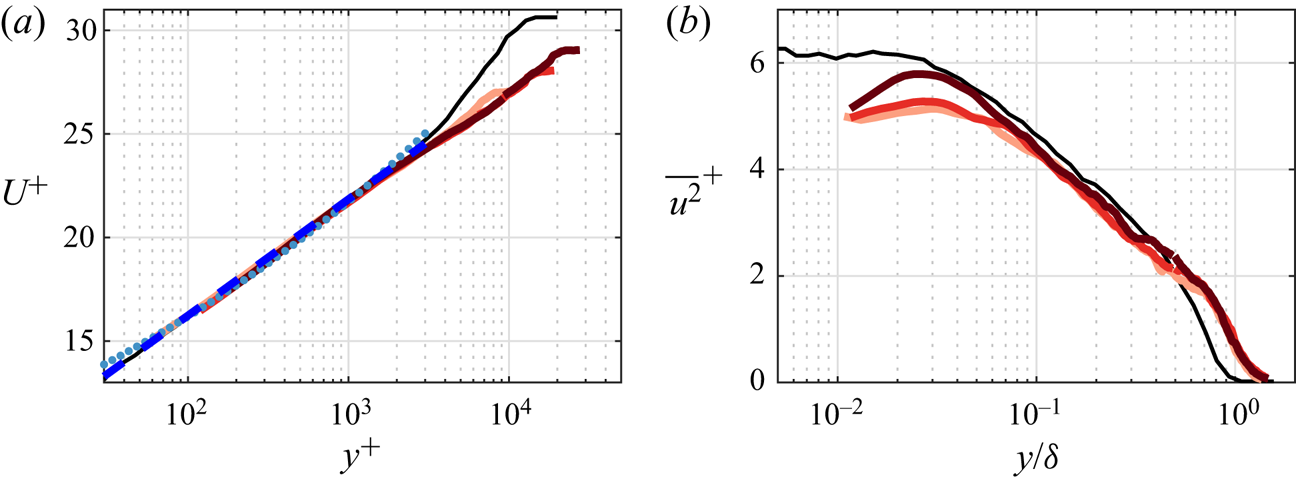
 $15\ \textrm {m}\,\textrm {s}^{-1}$) at the measurement location 12.5 m downstream of the trip. Wall-normal profiles of the streamwise velocity for the unladen flow are presented in figure 1(a) normalized by viscous units. The friction velocity is obtained by fitting the data with the log law (1.1) represented by the dashed blue line, obtaining
 $Re_\tau = 7000$, 13 000 and 19 000 for the increasing free-stream velocities. While these values are orders of magnitude lower compared to atmospheric flows, they are sufficient to ensure the scale separation indicative of high-Reynolds-number wall turbulence (Smits, McKeon & Marusic Reference Smits, McKeon and Marusic2011). For comparison, a canonical turbulent boundary-layer profile at
 $Re_\tau = 14\,000$ (Hutchins et al. Reference Hutchins, Nickels, Marusic and Chong2009, black line) and the power law (1.2, dotted blue line) are also included. The present measurements are accurately represented by the log law up to
 $y^+ = 2000$, which is the wall-normal limit for the two-phase measurements. The power law provides a slightly worse fit over the expected logarithmic region, showing significant departure in the near-wall and outer regions. The latter (roughly
 $y^+ > 2000$) deviates from the canonical turbulent boundary layer in that it does not possess a well-developed wake region, likely due to the strong tripping (Rodríguez-López, Bruce & Buxton Reference Rodríguez-López, Bruce and Buxton2016). Given that the two-phase measurements used in this study are performed at
 $y^+ < 2000$ only, this is not expected to influence the present results. The streamwise Reynolds stresses for the three Reynolds number are compared to Hutchins et al. (Reference Hutchins, Nickels, Marusic and Chong2009) in figure 1(b). The velocity fluctuations deviate from the canonical case in the outer region, where an increase in turbulent activity is also attributed to the strong tripping. Near the wall the present turbulent fluctuations are lower than expected, likely due to the limited resolution of the particle image velocimetry (PIV) measurements to be discussed below.
Wall-normal profiles of (a) streamwise time-averaged velocity and (b) streamwise Reynolds stress for  $Re_\tau = 7000$, 13 000 and 19 000 (red lines, darkness increases with
 $Re_\tau$. Results are compared to a canonical boundary layer at
 $Re_\tau = 14\,000$ from Hutchins et al. (Reference Hutchins, Nickels, Marusic and Chong2009) given by the black lines. The dashed and dotted blue lines indicate the log law and power law given by (1.1) and (1.2), respectively.

The flow is seeded simultaneously with flow tracers ( $1\text {--}2 \ \mathrm {\mu }\textrm {m}$ oil droplets) and inertial particles. The latter are size-selected glass spheres (Mo-Sci Corp.) with mean diameters of
 $d_p = 30$, 50 and
 $100\ \mathrm {\mu }\textrm {m}$ and a density of
 $\rho _p = 2500\ \textrm {kg}\,\textrm {m}^{-3}$, characterized in Petersen, Baker & Coletti (Reference Petersen, Baker and Coletti2019). To calculate their
 $\tau _p$, we base
 $Re_p$ on the mean slip velocity measured by two-phase imaging. Using the still-air settling velocity (as done in most previous studies) would lead to a slight quantitative difference in the value of
 $\tau _p$. The particles are injected into the boundary layer at the spanwise centreline of the wind tunnel, downstream of the boundary-layer trip and 11.3 m upstream of the measurement location. Particles are injected in the form of a mixture of air and particles via a seeding tube. The particle-laden air stream (negligibly small compared to the air flow rate through the wind tunnel) is supplied by a compressed air line which receives particles through a T-junction fed by a funnel filled with particles, located outside the wind tunnel. The particle injection rate can be controlled by changing the funnel orifice size and adjusting the air flow rate. To minimize intrusiveness, the seeding tube is connected through the wind-tunnel floor to a 15 cm tall airfoil-shaped injector. The particle-laden stream travels through the injector and is issued in the main stream in the co-flow direction by a cylindrical protrusion (1 cm in diameter) behind the airfoil trailing edge, approximately 7 cm from the wall. The particle-laden air flow profiles show now sign of the injector wake, and visual evidence of particles spreading across the full wind tunnel width confirms that the distance between injection and measurement is sufficient for dispersing the particles (supporting the approximation
 $\partial /\partial z = 0$). It is verified that the particle-laden flow is in approximate equilibrium, with no particle accumulation on the wall, no measurable variation of the statistics in the streamwise direction or in time (during the several minute duration of each run), and a vertical flux of particles too small to be measured. We remark, however, that the present accuracy in measuring the vertical particle velocity is limited, and so is the streamwise extent of the field of view. Nevertheless, given the relatively large fetch of the boundary layer compared to its thickness, and the small response time of the particles compared to their time of flight in the test section, the influence of possible streamwise development on the present data is considered small.
2.2. Measurement approach
Planar measurements are performed in the streamwise/wall-normal plane at the mid-span of the wind tunnel. The flow is illuminated by a Big Sky dual-pulse 200 mJ Nd:YAG laser, synchronized with two TSI Powerview 4MP cameras. Both cameras are fitted with 200 mm focal length lenses and are placed side by side, creating a field of view of approximately 50 mm (wall-normal) by 100 mm (streamwise) with a resolution of 32 pixels per mm. This covers the bottom 10 % of the boundary layer which contains most of the inertial particles due to the steep decay of concentration with wall-normal height. Image pairs are recorded with a separation time between the two pulses set to obtain a particle displacement of roughly 10 pixels; this is chosen to limit the uncertainty in air velocity due to pixel locking, while still being able to track inertial particles across image pairs. The sampling frequency is 7.25 Hz, which provides approximately uncorrelated realizations as there is at least one boundary layer turnover time  $\delta /U_\infty$ between realizations. Two runs of 1000 image pairs are recorded by each camera for each investigated case. As no measurable streamwise variation is present, the wall-normal profiles are averaged in the
 $x$-direction. Most of the presented data are binned in the wall-normal direction using logarithmically spaced bins. Given the roughly logarithmic profile of the concentration, the number of particles in each bin is of the same order of magnitude, leading to similar convergence of the statistics at each wall-normal location.
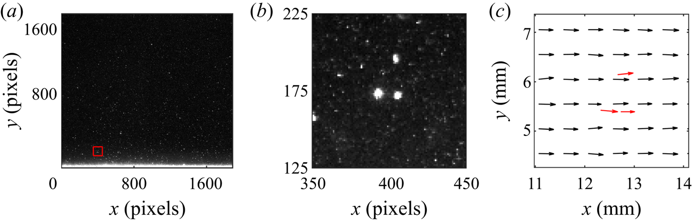
Simultaneous PIV and particle tracking velocimetry (PTV) are performed on the tracers and inertial particles, respectively. An example of a raw image and resulting velocity field is presented in figure 2. The processing procedure (discussed in detail in Petersen et al. (Reference Petersen, Baker and Coletti2019)) consists of the following steps: (i) separation of particle-only images from tracer-only images, (ii) processing of the tracer-only images by PIV, (iii) processing of the particle-only images by PTV using the cross-correlation approach, (iv) interpolation of the instantaneous PIV velocity vectors to the particle locations. Here we use an initial PIV interrogation window of 64 by 64 pixels, followed by a final step of 32 by 32 pixels with 50 % overlap, for a final vector spacing of 0.5 mm. The fluid velocity is interpolated to particle locations using weighted linear interpolation of the four neighbouring velocity vectors. A comparison with cubic and spline interpolation showed no significant difference in the results. The imaging parameters are adjusted to give streamwise particle displacements of about 10 pixels. The vertical velocity of the inertial particles is much smaller, its expected magnitude being of the order of the still-air settling velocity or 0.05–0.46 pixels. This is of the same order as the accuracy on the particle position, and therefore we do not report on the vertical velocities. Neither does our measurement approach (based on dual-pulse snapshots as opposed to time resolved) enable us to evaluate particle–wall collisions.
Examples of raw data and velocity field for the case with  $50\ \mathrm {\mu }\textrm {m}$ particles. (a) Raw image with the wall visible at the bottom (
 $y=0$), (b) zoomed in portion of (a), corresponding to the red square, (c) vector field corresponding to the portion of the image shown in (b) with the fluid vectors in black and the velocity of the three observed particles overlaid in red.

2.3. Parameter space
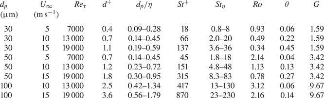
The parameter space for the present study is formed by a matrix of three particle sizes and three free-stream velocities. As we focus on fully suspended particles, we present only eight cases because the one with largest particles and lowest velocity resulted in deposition on the wind-tunnel floor. Especially for the higher  $St^+$, the particles travelling in the vicinity of the wall possibly collide with it, although our measurements cannot capture those events. Because there is no particle bed, collisions would not mobilize other deposited particles; nor are there shear-driven lift-off events of deposited particles. Thus, the dynamics is fundamentally different from what is commonly termed saltation in aeolian or sediment transport. For comparison of the parameter space in the present study to common regimes in sediment transport we use the Shields parameter (
 $\theta = U_\tau ^2/((\rho _p/\rho _f - 1)g d_p)$) and Galileo number (
 $G = d_p \sqrt {(\rho _p/\rho _f - 1)g d_p}/\nu$) as provided in table 1. Following the framework in Finn & Li (Reference Finn and Li2016), most of our cases are located in regime II, for which particle transport is dominated by gravitational settling. The exception are the two cases with
 $St^+ = 18$ and
 $St^+ = 45$ located in regime I for which no motion occurs in a bedform. It should be noted that in contrast to this framework, all our particles remain suspended and no particle bed is formed. This is possibly because such framework is developed for sediment transport in water.
Relevant dimensional and non-dimensional parameters for each case investigated in the present study. Kolmogorov scales  $\eta = (\nu ^2/\varepsilon )^{1/4}$ and
 $\tau _\eta = (\nu /\varepsilon )^{1/2}$ are based on the approximation
 $\varepsilon = U_\tau ^3/(\kappa y)$ in the logarithmic region.

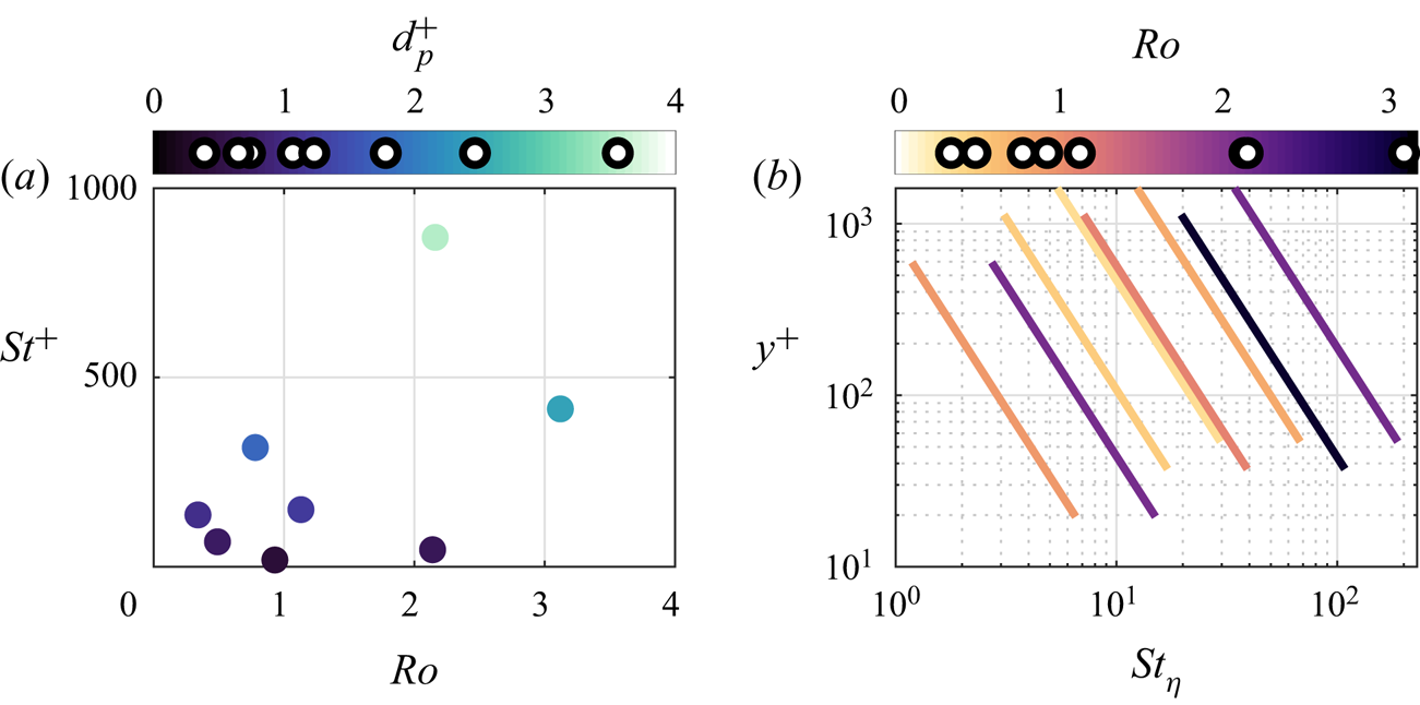
Figure 3(a) illustrates the parameter space in viscous units, while table 1 uses both viscous and Kolmogorov scaling. To define the Kolmogorov scales, we estimated the turbulent kinetic energy dissipation as  $\varepsilon = U_\tau ^3/(\kappa y)$ (Pope Reference Pope2000), considering that virtually all our data are in the logarithmic layer. As
 $\varepsilon$ varies across the boundary layer, table 1 provides ranges and figure 3(b) presents
 $St_\eta$ as function of wall-normal location. Even at the lowest location, the particle volume fraction is very low (approximately
 $10^{-6}$ or less). No measurable difference is found in the fluid velocity between the particle-laden flow cases and the unladen flow presented in figure 1, confirming that all considered cases are in the one-way-coupled regime.
Overview of parameter space. (a) Map of viscous-scaled Stokes number versus Rouse number, coloured by viscous-scaled particle diameter. (b) Distribution of Kolmogorov-scaled Stokes number as a function of wall-normal location.

3. Results
3.1. Wall-normal concentration profiles
3.1.1. Comparison with the Rouse–Prandtl model
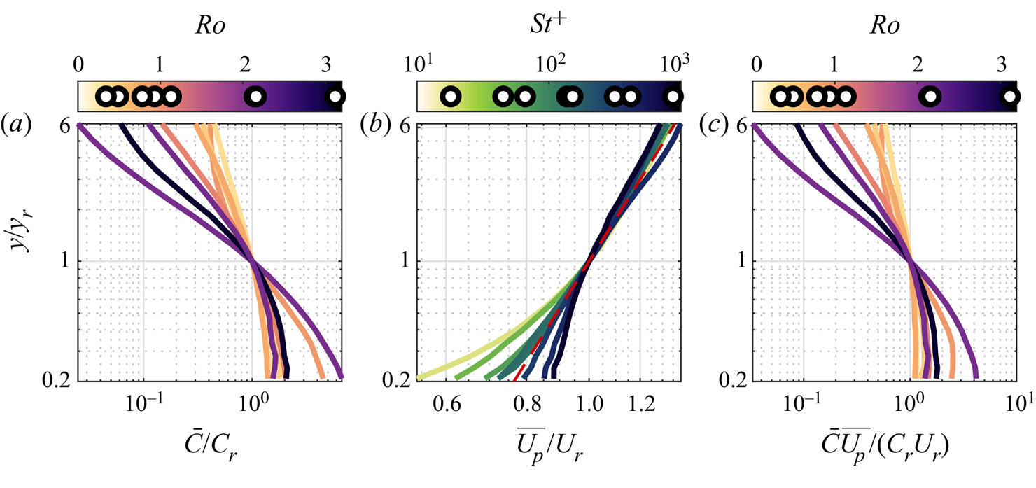
Wall-normal profiles of particle concentration, streamwise particle velocity and streamwise particle flux are presented in figure 4(a–c), respectively. All profiles are normalized by the values at a reference height  $y_r$, which is chosen as the logarithmic mid-point of our measurement window. In the context of the Rouse–Prandtl model, concentration, velocity and flux profiles are to be compared with the power-law expressions in (1.8), (1.2) and (1.9), respectively. The concentration profiles (figure 4a) display steeper wall-normal variation with increasing Rouse number, as expected from (1.8). The latter predicts a constant slope, while the measurements show deviations both at the lower and upper limit of the measurement window. The streamwise velocity profiles (figure 4b) roughly follow the power-law description (indicated by the red dashed line) in the outer region, with small deviations that can be ascribed to the log-law/power-law dichotomy (see figure 1a). The velocity discrepancies near the wall are much larger, and show a clear dependence with Stokes number: particles with
 $St^+$ smaller/larger than
 ${\sim }100$ move slower/faster than the power-law prediction. The streamwise flux (figure 4c) is taken as the product of mean concentration and mean velocity (streamwise turbulent fluxes being negligible in comparison). Following the power-law approximation (1.9), the expected flux slope is
 $\alpha -Ro$. For
 $\alpha \approx 1/6$, for most cases
 $Ro \gg \alpha$ and the profile shape is dominated by the concentration trend, as observed in our measurements.
Wall-normal profiles of (a) particle concentration, (b) streamwise particle velocity and (c) streamwise particle flux. Wall-normal profiles are normalized using reference values and presented on double-logarithmic axes. Concentration and flux profiles are coloured by Rouse number while velocity profiles are coloured by Stokes number. In panel (b), the dashed line indicates the power-law profile with  $\alpha = 1/6$.

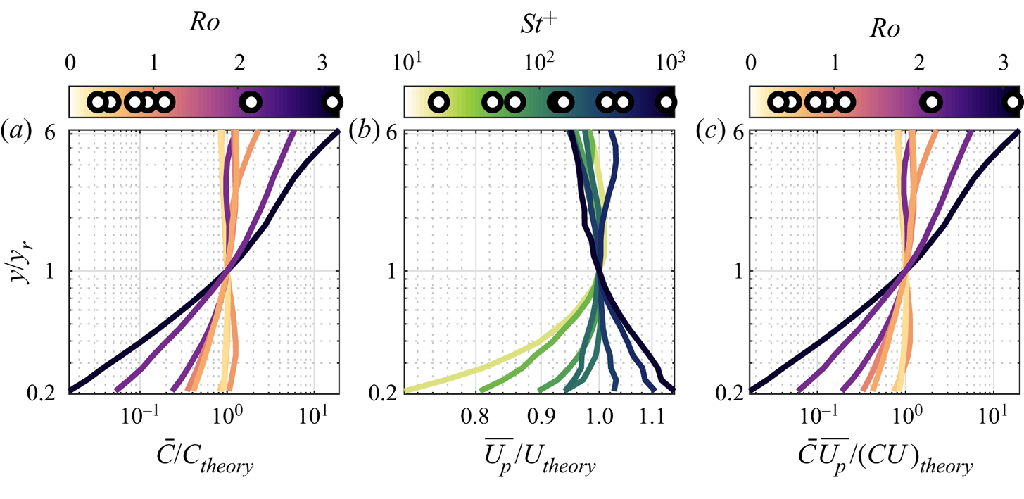
A more quantitative comparison with the power-law expressions is provided by taking the ratio of the power-law expressions, see figure 5. The measured concentrations (figure 5a) are within 20 % of the prediction for the two cases with  $Ro < 0.5$, but order-of-magnitude departures are found for higher
 $Ro$. The velocity profile above
 $y_r$ is within few per cent of the prediction, and near the wall the deviations can reach 30 %. This is substantial, considering that the overall velocity variation in the measurement window is around a factor two. Still, the variance in concentration is dominant and the flux comparison in figure 5(c) is almost indistinguishable from that in figure 5(a).


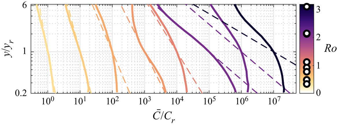
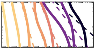
We now focus our attention on the wall-normal concentration and its gradient,  $\mathrm {d}\bar {C}/\mathrm {d}y$, which plays a crucial role in existing theories based on the eddy-diffusivity assumption. Figure 6 shows the same concentration profiles as in figure 4(a), straddling them horizontally by one decade each to highlight the departure from the Rouse–Prandtl prediction (dashed lines of the same colour). The two curves on the far right present by far the largest departure from the model. These are the cases with particles diameters
 $d_p = 100\ {\mathrm {\mu }}\textrm {m}$, which have the highest
 $St^+$ and appear as outliers in the
 $St^+$–
 $Ro$ plane (figure 3a). We will later discuss possible reasons for their behaviour.
Comparison of measured concentration profiles (solid lines) to power-law profiles (dashed lines). Each subsequent case is displaced to the right by a decade.

Focusing on the concentration gradient, the prediction of the Rouse–Prandtl model
 \begin{equation} {-}\frac{\mathrm{d}\bar{C}}{\mathrm{d}y}\frac{y}{\bar{C}} = Ro \end{equation}
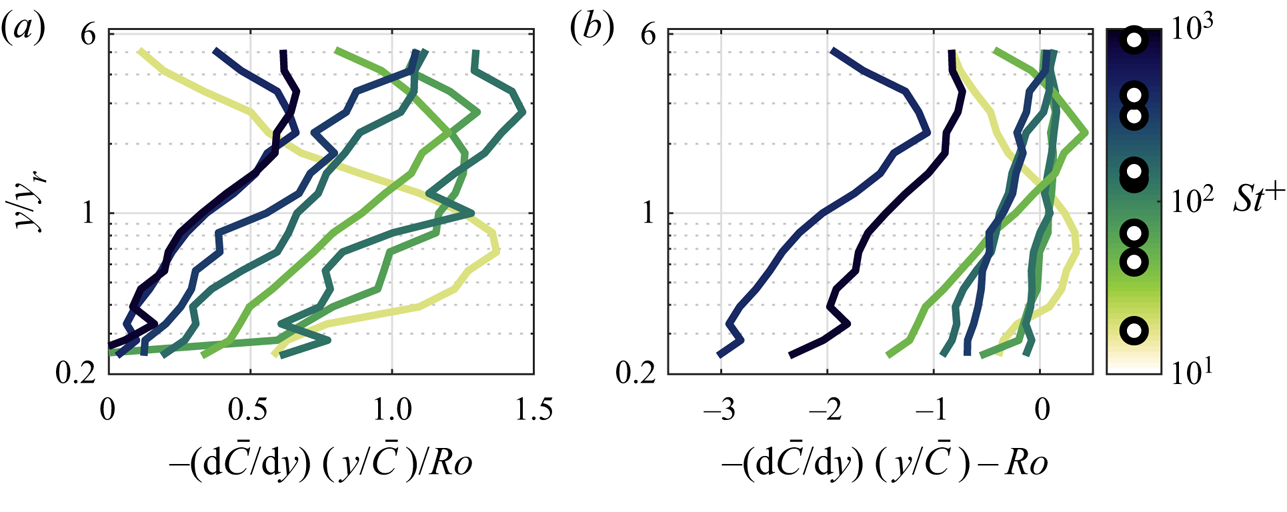
is tested in figure 7(a), which displays profiles of  $-\mathrm {d}\bar {C}/\mathrm {d}y(y/\bar {C})/Ro$. Beyond some experimental scatter, for most cases this non-dimensional slope grows moving away from the wall up to a peak close to the Rouse–Prandtl prediction of unity, and then decreases in the outer part of the measurement window. The colour coding highlights a dependency on Stokes number, which is made more evident by plotting the difference
 $-\mathrm {d}\bar {C}/\mathrm {d}y(y/\bar {C})-Ro$ (figure 7b). This reveals how the higher
 $St^+$ cases tend to deviate further from the theory, with a weaker concentration gradient compared to the lower
 $St^+$ cases.
Non-dimensional concentration gradient, normalized to equal (a) unity and (b) zero according to the Rouse–Prandtl model.

3.1.2. Roots of the departure from the power-law profile
As discussed in the introduction, the power-law profile is obtained as a solution of the advection–diffusion equation (1.7) by making assumptions about the particle settling velocity  $\overline {V_p}$, the particle wall-normal diffusivity
 $\varepsilon _y$ and the net vertical particle flux
 $\phi$. Because these three quantities are hard to measure accurately, we use the concentration profile to evaluate the impact of different assumptions on them. The assumptions made by Rouse and Prandtl are especially simple (hence powerful) but likely to be violated, to different degrees, in real flows. Alternatively, one can posit general trends for
 $\overline {V_p}$,
 $\varepsilon _y$ and
 $\phi$ and obtain alternative solutions to the advection–diffusion equation. We start by rearranging the advection–diffusion equation (1.7) as
 \begin{equation} {-}\frac{\mathrm{d}\bar{C}}{\mathrm{d}y} \frac{y}{\bar{C}} = \frac{-\overline{V_p} + \phi/\bar{C}}{\varepsilon_y/y}. \end{equation}
We can re-write (3.2) with each term in non-dimensional form as
 \begin{equation} {-}\frac{\mathrm{d}\bar{C}}{\mathrm{d}y} \frac{y}{\bar{C}} \frac{1}{Ro} = \frac{-\overline{V_p}/v_s + \phi/\phi_s}{\varepsilon_y/\varepsilon_0}, \end{equation}
where  $v_s = \tau _p g$ (or some constant value),
 $\phi _s = \bar {C}v_s$ and
 $\varepsilon _0 = \kappa U_\tau y$. The Rouse–Prandtl model assumes
 $-\overline {V_p}/v_s = 1$,
 $\phi /\phi _s = 0$ and
 $\varepsilon _y/\varepsilon _0 = 1$. A larger settling velocity, a downward net flux and a suppressed diffusivity contribute to increasing the concentration gradient, and vice versa.
Let us now consider the case in which only a subset of the Rouse–Prandtl assumptions is retained. For example, we can allow a vertical variation of the settling velocity and use the classic assumptions on diffusivity and net flux to write
 \begin{equation} {-}\frac{\overline{V_p}}{v_s} \sim -\frac{\mathrm{d}\bar{C}}{\mathrm{d}y} \frac{y}{\bar{C}} \frac{1}{Ro}. \end{equation}
Similarly, one can allow for changes in diffusivity or flux and use the remaining assumptions to obtain, respectively
 \begin{gather} \frac{\varepsilon_y}{\varepsilon_0} \sim \left(-\frac{\mathrm{d}\bar{C}}{\mathrm{d}y} \frac{y}{\bar{C}} \frac{1}{Ro}\right)^{-1}, \end{gather}
 \begin{gather}\frac{\phi}{\phi_s} \sim -\frac{\mathrm{d}\bar{C}}{\mathrm{d}y} \frac{y}{\bar{C}} \frac{1}{Ro} - 1. \end{gather}
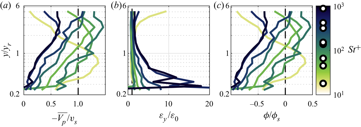
One can then compare the experimental results against the above estimates, to evaluate whether the observations are consistent with these respective scenarios. This is done in figure 8. The profiles of settling velocity depicted in figure 8(a) are based on (3.4) (and not on direct measurements of particle vertical velocity) and suggest a significant deviation from the still-air settling rate near the wall. Given that the turbulence is especially intense in this region, turbulence-driven changes in settling velocity are likely (Nielsen Reference Nielsen1993). On the other hand, figure 8(b) (based on (3.5)) displays order-of-magnitude deviations of the diffusivity near the wall, which is unrealistic even considering particle inertia and crossing trajectories (Wang & Stock Reference Wang and Stock1993). Finally, figure 8(c) (based on (3.6)) predicts significant negative fluxes near the wall, which is at odds with our observations of zero particle deposition. Therefore, as far as the near-wall region is concerned, the results lend some support to a scenario in which the Rouse–Prandtl assumptions on vertical diffusivity and net flux are tenable and the deviations from the power-law prediction are mainly the result of a local reduction in settling velocity.
Wall-normal profiles of required changes to the assumptions in the Rouse–Prandtl profile resulting from isolated changes in (a) vertical velocity, (b) diffusivity and (c) net flux.

Concerning the outer part of the measurement window, a variation of settling velocity with wall distance (figure 8a) is possible but seems unlikely, as the turbulent structure is not expected to change significantly in those strata of the boundary layer. Similarly, large changes in turbulent diffusivity (figure 8b) are not expected. On the other hand, a non-zero vertical flux (figure 8c) relatively far from the wall cannot be ruled out (Kind Reference Kind1992). Thus, one can speculate that deviations from the power-law profile near the top of the measurement window are largely the result of a negative net flux in this region, maintaining the usual assumptions on settling velocity and diffusivity. At intermediate distances from the wall, the deviations in concentration gradient are difficult to ascribe to any specific Rouse–Prandtl assumption. The general trend is that of a reduced slope (see figure 7), which according to (3.1) suggests an over-prediction of the Rouse number. Some variation in the Rouse number is expected as both the settling velocity and turbulent diffusivity have a high uncertainty as discussed in § 1.2. Instead of quantifying the Rouse number as  $Ro=\tau _p g/(\kappa U_\tau )$ (as done in the Rouse–Prandtl framework) we can define a more general effective Rouse number as
 $Ro^* = v_s/(\varepsilon _y/y)$. The variation observed in figure 7 at intermediate distances from the wall can then be ascribed to a discrepancy between
 $Ro^*$ and
 $Ro$.
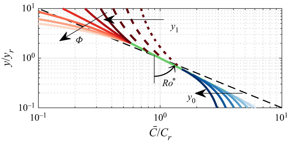
The above considerations, albeit speculative in nature, suggest simple modifications to the Rouse–Prandtl framework, leading to alternative solutions for the concentration profile. Here, we discuss a model which captures these considerations. We divide the boundary layer into three regions (near wall, intermediate and outer) separated by parametric locations  $y_0$ and
 $y_1$. We then assume a linearly increasing settling velocity for
 $y<y_0$ (
 $\overline {V_p} = -v_s y/y_0$), and a constant vertical net flux for
 $y>y_1$. (The latter requires relaxing the streamwise and/or spanwise homogeneity; as long as the flux is small, this does not conflict with the present observations.) Using these assumptions, the advection–diffusion equations for these three regions become
 \begin{gather} \bar{C} v_s \frac{y}{y_0} + \varepsilon_y \frac{\mathrm{d} \bar{C}}{\mathrm{d}y} = 0 \quad \textrm{for} \ y < y_0, \end{gather}
 \begin{gather}\bar{C} v_s + \varepsilon_y \frac{\mathrm{d} \bar{C}}{\mathrm{d}y} = 0 \quad \textrm{for} \ y_0 < y < y_1, \end{gather}
 \begin{gather}\bar{C} v_s + \varepsilon_y \frac{\mathrm{d} \bar{C}}{\mathrm{d}y} = -\phi \quad \textrm{{for}}\ y > y_1. \end{gather}
Assuming continuity of concentration across the layers, the resulting concentration profiles are given by
 \begin{gather} \frac{\bar{C}}{C_r} = \left(\frac{y}{y_r}\right)^{-Ro^*} \exp\left(-Ro^* \left[y/y_0 - 1 - {\log}(y/y_0)\right]\right) \quad \mathrm{for} \ y < y_0, \end{gather}
 \begin{gather}\frac{\bar{C}}{C_r} = \left(\frac{y}{y_r}\right)^{-Ro^*} \quad \textrm{for}\ y_0<y<y_1, \end{gather}
 \begin{gather}\frac{\bar{C}}{C_r} = \left(\frac{y}{y_r}\right)^{-Ro^*} + \varPhi \left(\left(\frac{y}{y_1}\right)^{-Ro^*}-1\right) \quad \textrm{for} \ y > y_1, \end{gather}
where  $\varPhi = \phi /(C_rv_s)$. The effect of varying the four parameters
 $Ro^*$,
 $y_0$,
 $y_1$ and
 $\varPhi$ is schematically illustrated in figure 9. We remark on relations with previously reported deviations from the power-law profile. Kind (Reference Kind1992) reported concentrations smaller than the power-law fit in the outer region and linked it to positive (upward) vertical fluxes, leading to (3.12). Vice versa, under net sedimentation, Zhu et al. (Reference Zhu, Pan, Wang, Liang and Ji2019) recently reported a sharp increase of concentration above the power-law profile in the outer region of a particle-laden turbulent boundary layer. They also found smaller near-wall concentration than predicted by the power-law profile, and so did Kiger & Pan (Reference Kiger and Pan2002). Instead, the point-particle simulations of Richter & Chamecki (Reference Richter and Chamecki2018) predicted an increase of settling velocity due to turbophoresis, producing near-wall increases of concentration. This is not captured by the present model form, which only includes hindered settling (to reproduce the present experimental results). Indirectly, this would suggest that our data do not support turbophoresis as a significant mechanism in the present regime. However, we warn that, on the one hand, turbophoretic and gravitational drift are inherently hard to distinguish in a horizontal flow; and on the other hand, quantitatively accurate predictions of turbophoresis are challenging in point-particle simulations (Wang et al. Reference Wang, Fong, Coletti, Capecelatro and Richter2019).
Modelled concentration profile following from expressions (3.10)–(3.12). Here,  $y_0/y_r$ is varied between 0.1 (light blue) to 0.6 (dark blue);
 $y_1/y_r$ is varied between 0.6 (dotted dark red line) to 2.0 (solid dark red line);
 $\varPhi$ is varied between 0.6 (dark red) to
 $-0.4$ (light red);
 $Ro^* = 0.8$ is kept constant in this schematic. A variation in
 $Ro^*$ changes the slope of the concentration profile, indicated by the dashed black line for
 $Ro^*=1.0$.

Using our measured concentration profiles, the model parameters in expressions (3.10)–(3.12) (i.e.  $Ro^*$,
 $\varPhi$,
 $y_0$ and
 $y_1$) are obtained from a least-square fit in which the fitted parameter is constant for a given profile. This fit leads to a good overlap between the measured and fitted concentration profiles with root-mean square errors between the two ranging from 3 % to 10 %. Normalized values of
 $Ro^*$,
 $\varPhi$,
 $y_0$ and
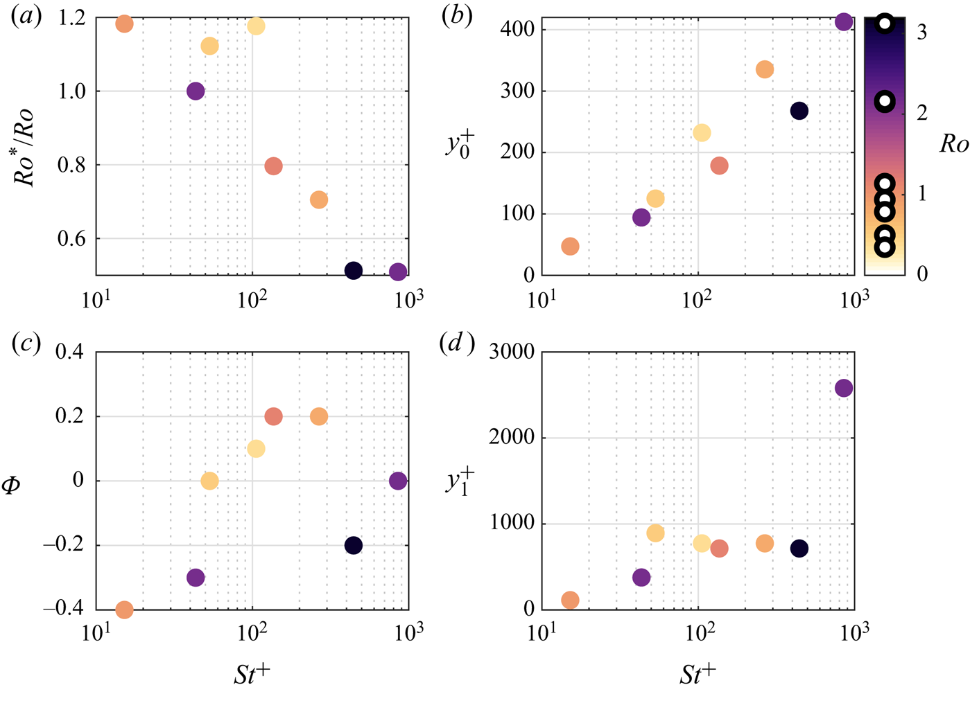
 $y_1$ are presented in figure 10. The effective Rouse number
 $Ro^*$ generally decreases with
 $St^+$ (figure 10a), with larger deviations from
 $Ro$ for the more inertial particles. Considering the role played by the Rouse number, this could indicate a reduced settling velocity and/or an increased particle diffusivity with increasing inertia. In general, this indicates that higher-
 $St$ particles depart more markedly from the Rouse–Prandtl model; this is expected as the latter does not explicitly account for particle inertia. The coefficient
 $y_0$, the wall-normal location below which the settling velocity decreases, shows an increasing trend with Stokes number (figure 10b). As the thickness of the layer
 $y<y_0$ is a manifestation of the wall influence, this suggests that the more inertial particles feel the effect of the wall at larger heights. This stands to reason, because more massive particles retain longer memory of their interaction with the wall. The parameters
 $\varPhi$ and
 $y_1$ (figure 10c–d) do not show clear trends within the present range of regimes. This could be due to the limited wall-normal extent of the measurement window, and/or the experimental uncertainty.
Fitted coefficients  $Ro^*$ (a),
 $y_0^+$ (b),
 $\varPhi$ (c) and
 $y_1^+$ (d) as functions of Stokes number and coloured by the Rouse number.

3.2. Slip velocity
3.2.1. Mean and particle-conditioned slip velocities
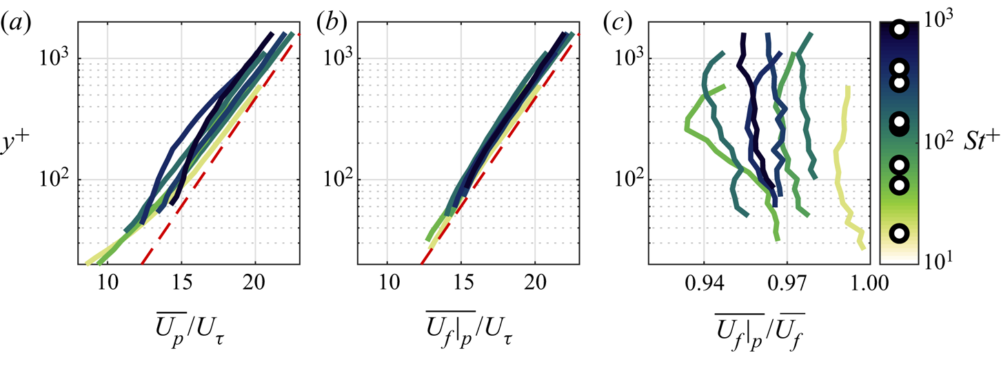
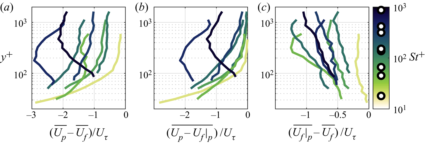
Wall-normal profiles of mean streamwise particle velocity are presented in figure 11(a), now in semilogarithmic axes. To limit clutter, the log law is plotted as a proxy for the fluid velocity of all cases. The particles consistently lag the fluid, i.e. the mean particle velocity is lower than the mean fluid velocity. The particle velocity  $\overline {U_p}$ can be written as the sum of the fluid velocity at the particle location (particle-conditioned fluid velocity,
 $\overline {U_f|_p}$) and the slip velocity with respect to it (
 $\overline {U_p - U_f|_p}$)
 \begin{equation} \overline{U_p} = \overline{U_f|_p} + \overline{U_p - U_f|_p}. \end{equation}
Wall-normal profiles of  $\overline {U_f|_p}$ are presented in figure 11(b). The particle-conditioned fluid velocity is everywhere lower than the mean (unconditioned) fluid velocity; that is, the inertial particles over-sample low-velocity regions of the flow. The ratio
 $\overline {U_f|_p}/\overline {U_f}$ is presented in figure 11(c):
 $\overline {U_f|_p}$ is 1 %–7 % smaller than the mean fluid velocity, with no clear dependence on the viscous Stokes number or wall-normal location.
Wall-normal profiles of (a) streamwise velocities of the particles, (b) the fluid sampled by the particles and (c) the fluid sampled by the particles relative to the unconditioned mean fluid velocity. The dashed red line indicates the log law which closely approximates the unconditioned mean fluid velocity.

The averaging operation prompts the distinction between two kinds of slip velocity: the difference between the mean particle velocity and the mean fluid velocity ( $\overline {U_p} - \overline {U_f}$) and the mean of the instantaneous slip velocity
 $\overline {U_p - U_f|_p}$. Following Kiger & Pan (Reference Kiger and Pan2002), we refer to the former as ‘mean slip velocity’ and the latter as ‘particle-conditioned slip velocity’. The mean and particle-conditioned slip velocities are presented in figures 12(a) and 12(b), respectively, normalized by the friction velocity. Both show similar trends, including a general increase with
 $St^+$. With the exception of the highest
 $St^+$ cases, the slip velocity increases in magnitude towards the wall. This behaviour can be ascribed to the decreasing time scales of the turbulent fluctuations approaching the wall (exemplified by the near-wall increase in
 $St_\eta$, see figure 3b) which the particles become unable to follow. In addition, we speculate that interactions of the particles with the wall will reduce their momentum near the wall (increasing the slip velocity). However, due to the limited spatial resolution, our present measurements are unable to capture such particle–wall interactions. The two highest
 $St^+$ cases show non-monotonic profiles, with a decrease in slip velocity approaching the wall. This is likely an effect of the massive particle inertia, enabling them to retain their streamwise speed when approaching the wall from more outer regions. Indeed, in vertical channels high-
 $St$ particles have been shown to even surpass the fluid velocity near the wall (Kulick, Fessler & Eaton Reference Kulick, Fessler and Eaton1994; Rouson & Eaton Reference Rouson and Eaton2001; Benson, Tanaka & Eaton Reference Benson, Tanaka and Eaton2004; Fong et al. Reference Fong, Amili and Coletti2019).
(a) Mean and (b) particle-conditioned slip velocities and (c) oversampling of fluid regions faster/slower than the mean, coloured by Stokes number.

We can rewrite (3.13) as
 \begin{equation} \overline{U_p} -\overline{U_f} = \overline{U_p - U_f|_p} + \overline{U_f|_p} - \overline{U_f},\end{equation}
which makes explicit the two contributions to the mean slip velocity: the particle-conditioned slip velocity ( $\overline {U_p - U_f|_p}$) and the oversampling of fluid regions faster/slower than the mean (
 $\overline {U_f|_p} - \overline {U_f}$). The latter term is plotted in figure 12(c), where negative values indicate that the particles favour low-speed regions. This oversampling is stronger away from the wall, in contrast to the particle-conditioned slip velocity that typically grows in magnitude approaching the wall. Both terms have similar magnitude. Indeed, although the crossing point varies case by case, a quantitative comparison indicates that near the wall the particle-conditioned slip velocity is larger than the preferential sampling term, and vice versa in the outer region. The significant particle-conditioned slip contrasts with the observations of Kiger & Pan (Reference Kiger and Pan2002) who found it negligible in their experiments. However, several differences with our case can explain the discrepancy, including their lower particle-to-fluid density ratio, smaller
 $Re_\tau$ and smaller
 $St$.
The stronger oversampling of low-speed regions away from the wall is noteworthy. It is at odds with the established picture that preferential concentration in wall-bounded flows is driven by accumulation of particles in low-speed streaks in the inner layer (see e.g. Kaftori et al. Reference Kaftori, Hetsroni and Banerjee1995a; Niño & Garcia Reference Niño and Garcia1996; Rouson & Eaton Reference Rouson and Eaton2001; Marchioli & Soldati Reference Marchioli and Soldati2002). Because past studies have focused on much lower  $Re_\tau$, it is possible that the present trend is linked to features specific to high-
 $Re$ turbulent boundary layers, such as very-large-scale motions (Marusic et al. Reference Marusic, McKeon, Monkewitz, Nagib, Smits and Sreenivasan2010). The latter have been recently shown to leave their footprint on inertial particle transport using numerical simulations (Zhang, Hu & Zheng Reference Zhang, Hu and Zheng2018; Wang & Richter Reference Wang and Richter2019). Indeed, the tendency of the particles to oversample slow fluid regions is displayed also by the largest
 $St^+$ particles, which are expected to be ballistic with respect to the viscous scales characterizing the near-wall dynamics. Their behaviour indicates a response to large eddies associated with relatively long time scales.
3.2.2. Scaling of the instantaneous slip velocity with local flow conditions
The multiscale nature of the high- $Re$ turbulent boundary layer provides the opportunity of evaluating the particle response over a wide range of local
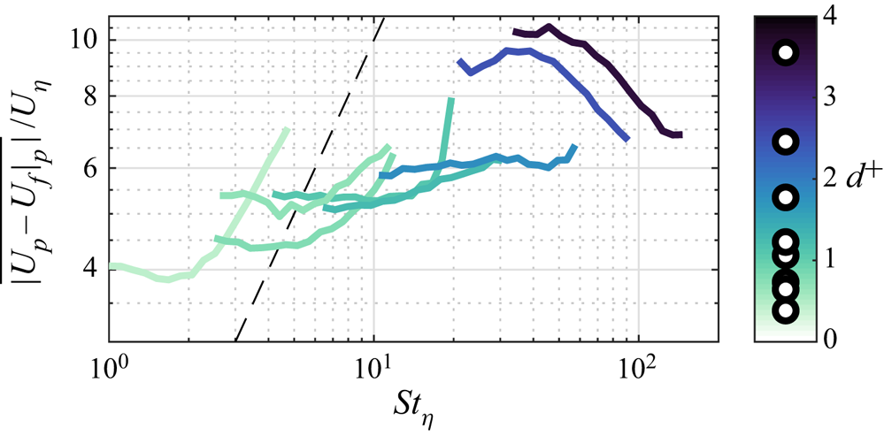
 $St_\eta$ (see figure 3b). The assumption that the particle motion is dictated by the surrounding fluid is the basis of the equilibrium Eulerian approach as proposed by Ferry & Balachandar (Reference Ferry and Balachandar2001) building on the seminal work of Maxey (Reference Maxey1987). This was later used by Balachandar (Reference Balachandar2009) to derive the scaling of the slip velocity in various regimes. For heavy particles with
 $St_\eta$ in the inertial range (i.e. with response time between the Kolmogorov and integral time scale), he obtained
 \begin{equation} \frac{\overline{|U_p - U_f|_p|}}{U_\eta} = St_\eta^{1/2}. \end{equation}
This assumes gravitational acceleration to be smaller than the Kolmogorov acceleration  $\varepsilon ^{3/4}/\nu ^{1/4}$, which is the case here. Equation (3.15) is plotted and compared to the present data in figure 13. The observed slip velocity for the least inertial particles approximately follows this prediction. Above
 $St_\eta = \textit{O}(10)$ the dependency with Stokes number is weaker. This could be a consequence of the response time of the particles approaching the upper end of the inertial range, which in the inner region of the boundary layer (where the higher
 $St_\eta$ is attained) is marginally separated from the dissipation range. The
 $100\ \mathrm {\mu }\textrm {m}$ particles show again an outlier behaviour, with the normalized slip velocity decreasing with
 $St_\eta$.
Instantaneous slip velocity normalized by Kolmogorov velocity scale as a function of the local Stokes number, coloured by particle size. The dashed line indicates equation (3.15).

The scaling of the slip velocity can also be analysed by considering the particle Reynolds number
 \begin{equation} Re_p = \frac{\overline{|U_p - U_f|_p|}d_p}{\nu},\end{equation}
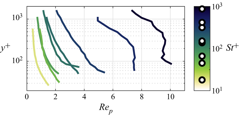
which is a key parameter in modelling the particle–fluid interaction. This is plotted as function of wall-normal location in figure 14. The least inertial particles have  $Re_p = \textit{O}(1)$, for which Stokesian drag with relatively small corrections is expected (Clift et al. Reference Clift, Grace and Weber2005). However, especially for the two most inertial cases,
 $Re_p$ is sufficiently large for nonlinearities to play a significant role, undermining the assumptions behind the particle equation of motion (Maxey & Riley Reference Maxey and Riley1983). Figure 15 explores the dependence of
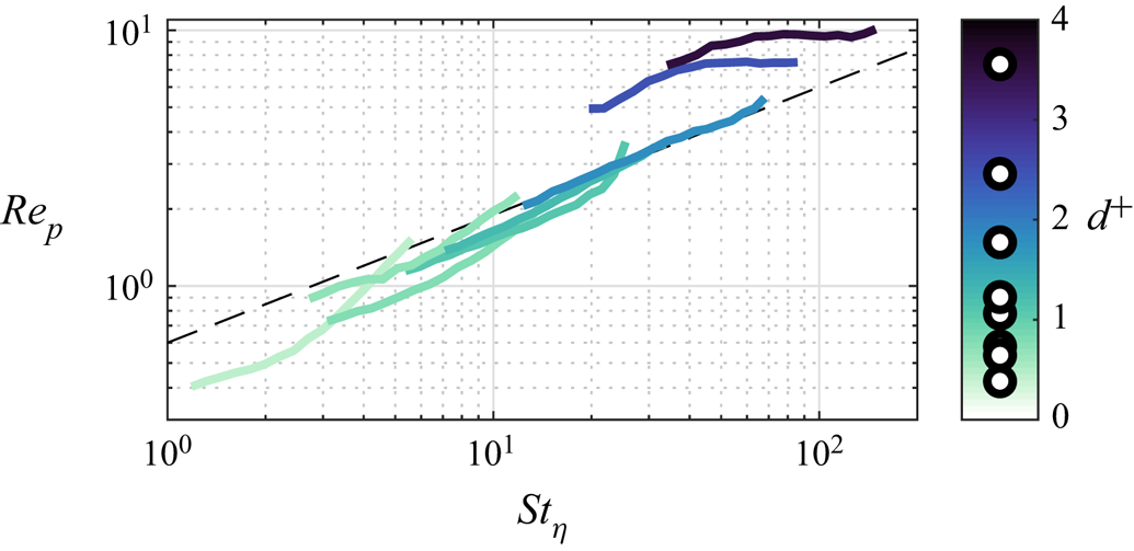
 $Re_p$ with the local Stokes number, and shows a remarkably good collapse over a single curve
 $Re_p = 0.6 St_\eta ^{0.5}$ for all but the two highest-
 $St$ cases. This collapse can be linked to (3.15) by substituting
 $\nu = \eta U_\eta$, i.e.
 $(\overline {|U_p - U_f|_p|}/U_\eta )( d_p/\eta ) = St_\eta ^{1/2}$. This points to the discrepancy, related to the particle size in Kolmogorov scales, between our measurements and the theoretical framework by Balachandar (Reference Balachandar2009). The two highest-
 $St$ cases display a plateau, suggesting that the maximum possible slip velocity is attained. As discussed in Balachandar (Reference Balachandar2009), the slip velocity of the heavy particles is expected to be capped by the velocity scale of the largest size eddies. This can be estimated as the square root of the peak streamwise Reynolds stress
 $\overline {u_f^2}|_{max}$. Thus, using the well-resolved measurements from Hutchins et al. (Reference Hutchins, Nickels, Marusic and Chong2009) at comparable
 $Re_\tau$ (where
 $\overline {u_f^2}|_{max} \approx 8.5 U_\tau ^2$), we expect the particles of
 $d^+ = 2.5$ and 3.6 to experience maximum Reynolds numbers based on the slip velocity of
 $Re_p \approx 7.2$ and 10.4, respectively; this is in close agreement with the plateaus in figure 15.
Mean particle Reynolds numbers based on the particle-conditioned slip velocity as defined in (3.16) as functions of wall-normal location, coloured by Stokes number.

Particle Reynolds number as a function of local Stokes number on (a) linear and (b) logarithmic axes, coloured by particle size. The dashed lines indicate the fitted power law  $Re_p = 0.6 St_\eta ^{0.5}$.

3.2.3. Particle-conditioned vertical velocity
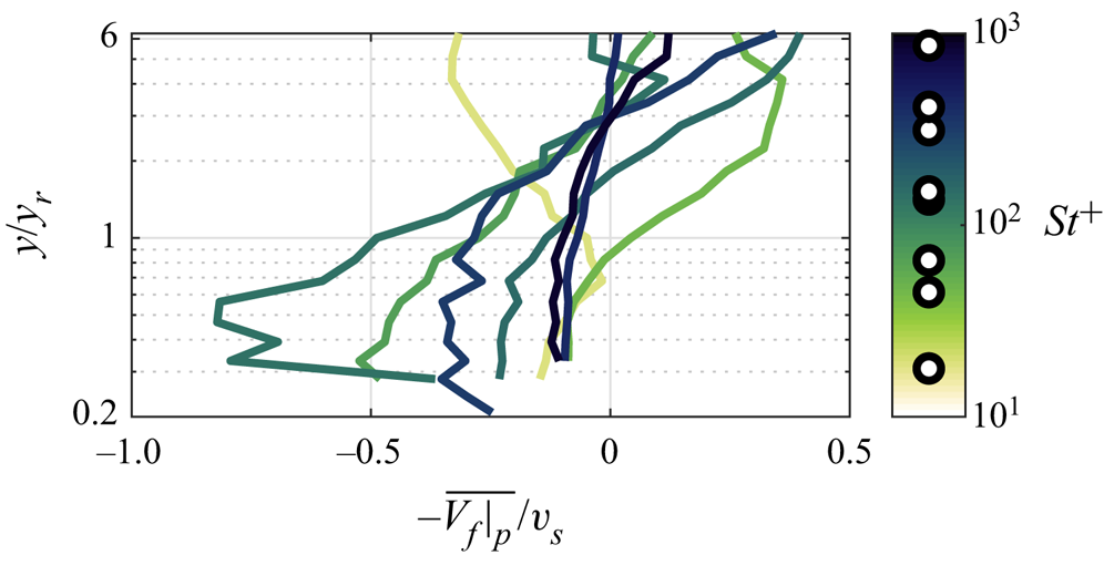
As discussed in § 2.2, the wall-normal particle velocity is not accurately measured in the present study. Although this prevents us from evaluating the slip velocity, we can evaluate the particle-conditioned fluid velocity,  $\overline {V_f|_p}$. This velocity sampled by the particles is of particular interest in relation to the particle settling velocity which influences the concentration profiles as discussed in § 3.1.2, specifically the deviation presented in figure 8(a). The wall-normal velocity sampled by the particles is presented in figure 16, normalized as
 $-\overline {V_f|_p}/v_s$, analogous to the normalization in figure 8(a). The variations in these two figures is qualitatively similar, suggesting that the reduced/increased settling velocity as hypothesized in figure 8(a) is linked to sampling of upward/downward fluid velocity fluctuations.
Wall-normal profiles of wall-normal fluid velocity sampled by the particles, coloured by Stokes number. Normalization is analogous to figure 8(a), with negative velocities away from the wall and positive velocities towards the wall.

3.3. Particle-conditioned flow topology
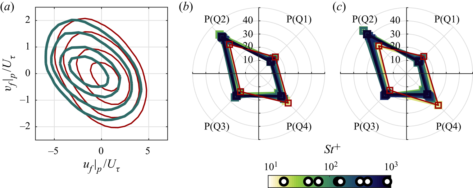
To gain insight in the particle–turbulence interactions, we explore the flow events experienced by the particles. We begin by performing a quadrant analysis of the particle-conditioned fluid velocity fluctuations. Joint probability density functions (JPDFs) of the streamwise and wall-normal components are presented in figure 17(a) for the case with  $St^+ = 151$, which is representative of all investigated cases. The tendency of the particles to favour
 $u_f < 0$ regions is apparent, consistent with the results in § 3.2.1. The shape of the JPDFs indicates the prevalence of events contributing to negative Reynolds shear stresses, as expected in turbulent shear flows. However, the comparison with the unconditioned fluid velocity highlights the tendency of the particles to over-sample events in the second quadrant Q2 (where
 $u_f < 0$ and
 $v_f > 0$, classically referred to as ejection events) and under-sample those in the fourth quadrant Q4 (
 $u_f > 0$ and
 $v_f < 0$, referred to as sweeps). This agrees with findings by Kiger & Pan (Reference Kiger and Pan2002). Figures 17(b) and 17(c) compare the percentage of particle-conditioned events in the four quadrants for the different cases and at two wall-normal locations. Preferential sampling of ejections over sweeps appears increasingly dominant for the smaller
 $St^+$ and at larger distances from the wall. This is especially interesting, because these are conditions for which
 $St_\eta = \textit{O}(1)$. In shear-less turbulence one would expect such particles to strongly oversample downward region of the flow as consequence of preferential sweeping (Wang & Maxey Reference Wang and Maxey1993; Petersen et al. Reference Petersen, Baker and Coletti2019). This is not the case here, even in the outer region of the boundary layer where mean shear is moderate. A possible explanation is that preferential sweeping is offset by the tendency of the particles to favour
 $u_f < 0$ events: because these are statistically correlated to
 $v_f > 0$ events, particles are more likely to be found in upward-moving flow regions.
(a) Joint probability density functions of horizontal and vertical velocity fluctuations for the fluid (red lines) and particle-conditioned fluid (green lines) for the  $St^+ = 151$,
 $Ro = 1.13$ case with contours at levels 0.01, 0.02, 0.04 and 0.06. (b) Probability of particle-conditioned fluid events in each quadrant for the wall-normal bin at
 $y = 8$ mm, unconditioned fluid is indicated by the red line. (c) Same as (b) for a wall-normal location of 37 mm.

Preferential sampling of inertial particles can also be characterized in terms of the fluid velocity gradient (Squires & Eaton Reference Squires and Eaton1991a). We discriminate between rotation-dominated and strain-dominated regions using the second invariant of the velocity gradient tensor (Hunt, Wray & Moin Reference Hunt, Wray and Moin1988)
 \begin{equation} Q = \omega^2/4 - s^2/2, \end{equation}
where  $\omega ^2 = 2\,\mathrm {tr}(\boldsymbol {\varOmega }^2)$ is the enstrophy,
 $s^2 = \mathrm {tr}({\boldsymbol {S}}^\textbf {2})$ is the squared strain rate and
 ${\boldsymbol {S}}$ and
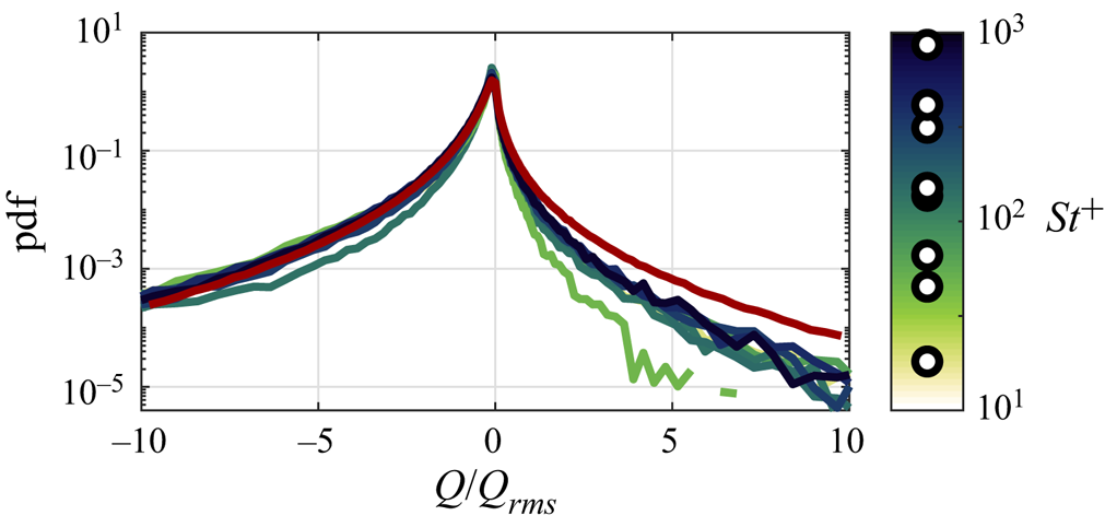
 $\boldsymbol {\varOmega }$ are the symmetric and anti-symmetric parts of the velocity gradient tensor, respectively. Due to the planar nature of the present measurements, we can only consider the reduced form of the full velocity gradient tensor, formed by its in-plane components. While this is not sufficient to fully describe the flow topology (Perry & Chong Reference Perry and Chong1994), the reduced tensor can provide important physical insight into the properties of high-enstrophy and strain-rate structures (Cardesa et al. Reference Cardesa, Mistry, Gan and Dawson2013; Rabey, Wynn & Buxton Reference Rabey, Wynn and Buxton2015) and reproduces the essential small-scale features of the turbulence (Fiscaletti, Ganapathisubramani & Elsinga Reference Fiscaletti, Ganapathisubramani and Elsinga2015; Carter & Coletti Reference Carter and Coletti2018). Figure 18 shows the PDF of
 $Q$ evaluated at the particle locations. Compared to the unconditioned fluid, the particle-conditioned distributions show a clear under-sampling of rotation-dominated regions (
 $Q > 0$), especially for the least inertial particles. This is consistent with the classic picture of particles being centrifuged out of vortex cores (Eaton & Fessler Reference Eaton and Fessler1994).
Probability density functions of ensemble-averaged  $Q$ for the particle-conditioned flow for all eight cases, coloured by Stokes number. The red line indicates the
 $Re_\tau = 7000$ unladen flow case, which displays insignificant differences from the other unladen cases.

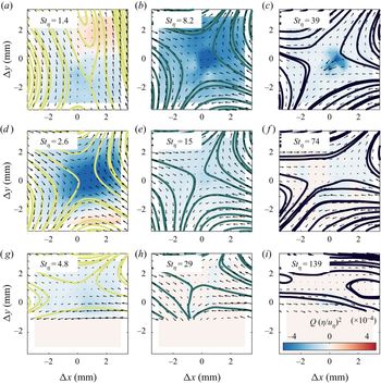
The above suggests that the particles sample turbulent flow regions with a specific topology. To illustrate it, we apply a Galilean decomposition of the particle-conditioned flow field (Adrian, Christensen & Liu Reference Adrian, Christensen and Liu2000a). Here, it is convenient to apply the Galilean decomposition to the fluctuations  $u$, which is free by the signature of mean shear by virtue of the Reynolds decomposition. The process is thus the following: (i) we consider the particle-conditioned fluid fluctuations
 $u_f|_p({\rm \Delta} x, {\rm \Delta} y)$, where
 ${\rm \Delta} x$ and
 ${\rm \Delta} y$ are the in-plane separations from the particle location; (ii) we subtract a convection velocity
 $U_c$ calculated as the local spatial average over a 6 mm by 6 mm window centred around each particle; (iii) we ensemble average over all particles within a range of wall-normal distances. The results are presented in figure 19 for
 $St^+ = 18$, 151 and 870 for three strata of the boundary layer; these capture the trend for the different cases, which are weakly sensitive to the specific choice of Galilean window size and wall-normal ranges. Streamlines and
 $Q$ fields indicate that, on average, the particles are found near the saddle point of a strain cell with forward-leaning extensive axis and backward-leaning compressive axis. This is consistent with Baker et al. (Reference Baker, Frankel, Mani and Coletti2017) who concluded that inertial particles falling in homogeneous isotropic turbulence favoured the saddle point of strain cells with vertical compressive axis. The inclination here is likely rooted in the prevalence of forward-leaning vortices in the turbulent boundary layers (Adrian, Meinhart & Tomkins Reference Adrian, Meinhart and Tomkins2000b) and the significant streamwise slip. In fact, for the least inertial particles in the outer region (figure 19a), the compressive axis is almost vertical, hinting to a similarity with homogeneous shear-less turbulence. In most other cases, however, the inclination of the strain cell is evident (the compressive axis making an angle
 ${\approx } 25^\circ$ with the horizontal). The contours of
 $Q$ and the quantitative analysis of the strain-rate tensor eigenvalues (not shown) indicate that tendency of oversampling this type of instantaneous structure is most pronounced for
 $St_\eta = \textit{O}(10)$.
Particle-conditioned velocity fields for particles located in the ranges  $1.5\ \textrm {mm}< y < 4\ \textrm {mm}$ (g–i),
 $7\ \textrm {mm} < y < 13\ \textrm {mm}$ (d–f ) and
 $24\ \textrm {mm} < y < 45\ \textrm {mm}$ (a–c) for the cases with
 $St^+ = 18$ (a–g),
 $St^+ = 151$ (b–h) and
 $St^+ = 870$ (c–i). Vectors and streamlines indicate velocity fields after applying both a Reynolds decomposition and a Galilean decomposition. Background indicates
 $Q$ (see (3.17)).

The topology of the particle-conditioned flow field strongly resembles the picture proposed by Kasbaoui, Koch & Desjardins (Reference Kasbaoui, Koch and Desjardins2018), where regions of excess strain in a perturbed shear flow accumulate particles by virtue of the compressibility of their velocity field (Maxey Reference Maxey1987). The latter argument is based on a small-Stokes-number assumption, which could appear at odds with the observed topology surviving even for relatively strong particle inertia. It is important, however, to consider the multi-scale nature of turbulence and its consequences for particle-laden flows. In shear-less turbulence, theoretical work from Goto & Vassilicos (Reference Goto and Vassilicos2006) and Yoshimoto & Goto (Reference Yoshimoto and Goto2007) and simulations from Bec et al. (Reference Bec, Biferale, Lanotte, Scagliarini and Toschi2010) and Ireland, Bragg & Collins (Reference Ireland, Bragg and Collins2016a,Reference Ireland, Bragg and Collinsb) showed that particles with  $St_\eta \gg 1$ are responsive to eddies up to the inertial range if these have time-scales comparable to the particle response time. Recent experiments from Petersen et al. (Reference Petersen, Baker and Coletti2019) demonstrated how clustering may even approach the integral scales. Here we do not attempt to identify clusters as the strong wall-normal gradient of concentration would bias the analysis; still, the ubiquity of the underlying preferential sampling points to the robustness of the phenomenon for a wide range of Stokes numbers. This breaks down only for the most inertial particles (
 $St_\eta > 100$) in the near-wall region (figure 19i), for which the flow pattern changes dramatically. The effect of the wall (possibly also through particle–wall collision) is dominant in those conditions, and a topological analysis is deferred to future studies reaching higher resolution.
4. Discussion and conclusions
The transport of inertial solid particles in a smooth-wall air turbulent boundary layer has been investigated experimentally. We consider a fully suspended regime close to equilibrium, and a mass loading sufficiently low that the particle back reaction on the fluid can be considered negligible. The friction Reynolds number is sufficient for high- $Re$ features of the flow to emerge, making the present results relevant to mechanisms at play in atmospheric flows. In particular, the wide range of investigated Stokes numbers makes the study relevant to the transport of both dust and sand in the surface layer. The canonical nature of the flow, however, ensures that the findings have wide applicability to a wealth of settings in the environmental and industrial realms. The relatively small particle sizes (in a regime that is routinely tackled by point-particle simulations) allow for direct comparisons with future numerical studies. Leveraging simultaneous imaging of both inertial particles and air motion, we have focused on long standing but still unresolved aspects of this class of flows: the equilibrium profiles of the particle concentration, the particle-fluid slip velocity, and the preferential sampling of fluid flow regions by the particles.
A detailed comparison has been performed between the experimental observations and the classic theory of Rouse (Reference Rouse1937) and Prandtl (Reference Prandtl1952) especially in terms of the particle concentration, which for these regimes largely determines the trend of the streamwise fluxes. This provides insight into the respective impact of the different hypotheses behind the theoretical framework. Previous efforts aimed at critically evaluating the Rouse–Prandtl model were mostly based on field measurements (with naturally large experimental scatter) and numerical simulations (with somewhat restrictive simplifications in the flow modelling). The present experiments indicate that particles generally display weaker wall-normal gradients of concentration compared to the Rouse–Prandtl equilibrium model (in its power-law form). This is visible in different regions of the boundary layer, and is attributed to a combination of mechanisms: at relatively small distances from the wall, the concentration is smaller compared to the power-law profile, probably due to near-wall turbulence hindering the settling velocity of the particles; away from the wall, concentrations are larger than predicted by the theory, possibly because of a small net downward flux in our experiment. In general, the more inertial particles show a larger departure from the Rouse–Prandtl model (see figure 6); the latter does not explicitly account for particle inertia, underscoring the need for a more general theory capable of amending this limitation. While such step is not attempted here, we propose a simple three-layer parameterization of the concentration profile with built-in particle inertia effects. It highlights some of the main trends, including that the influence of the wall extends to greater heights for particles of larger inertia. The parameterization captures previously reported behaviours, but it is still to be quantitatively tested against extensive data sets.
The particles are found to lag the fluid across the boundary layer, with a mean slip velocity of the order of the friction velocity, increasing with particle inertia and generally increasing approaching the wall. Near the wall, the mean slip is largely due to a significant particle-conditioned slip velocity, i.e. the instantaneous slip of the particles relative to the surrounding fluid. Away from the wall, the larger contributor to the mean slip is instead the preferential sampling of low-speed fluid regions. This picture departs from the commonly held view, in that the accumulation of particles in low-speed regions is usually associated with streamwise vortices and low-momentum streaks in the inner layer. This view, however, relies on observations of low-Reynolds-number flows (typically  $Re_\tau = \textit{O}(10^2)$). It is then hypothesized that the present results are an indication of high-
 $Re$ features of wall-bounded turbulence (such as very-large-scale motions) playing an increasingly important role on the particle transport in the present regime (
 $Re_\tau = \textit{O}(10^4)$), as compared to near-wall streaks known to follow inner scaling. This would have far-reaching consequences, since flows of environmental and industrial relevance can have Reynolds numbers several orders of magnitude larger yet. The present measurements have a limited streamwise extent and cannot ascertain whether the large-scale motions contribute to organize the particles in correspondently large structures. Thus, this hypothesis needs to be verified in future studies using much larger imaging windows.
The scaling of the instantaneous slip velocity with respect to the local flow conditions is explored in the framework of the equilibrium Eulerian approach. In agreement with the latter, the slip velocity normalized by the local Kolmogorov velocity generally grows with  $St_\eta$; the dependence is relatively weak, however, and the slip velocity reaches a plateau for
 $St_\eta = \textit{O}(10)$. This suggests that the more inertial particles in the considered range have response times approaching or exceeding the integral time scales of the turbulence (Balachandar Reference Balachandar2009). This is confirmed by the trend of particle Reynolds number based on the instantaneous slip velocity, which collapse on a curve
 $Re_p \propto St_\eta ^{0.5}$ before plateauing for the largest particles (
 $d_p = 100\ \mathrm {\mu }\textrm {m}$). The latter have
 $Re_p = \textit{O}(10)$, significantly larger than the other cases, they occupy removed locations in the
 $St^+$–
 $Ro$ parameter space, and display an outlier behaviour both in terms of concentration profile and slip velocity. The reason of their qualitatively different interaction with the flow is most likely rooted in the substantial nonlinear drag impacting their motion, or possibly a finite-size effect. The latter possibility is unlikely, though: their size is only a few wall units while their behaviour is peculiar even far away from the wall, where they are much smaller than any flow scale.
It is noteworthy that qualitative differences in aeolian transport properties have long been remarked between grains smaller and larger than  $70\ \mathrm {\mu }\textrm {m}$, conventionally labelled as dust and sand, respectively (Bagnold Reference Bagnold1941; Tsoar & Pye Reference Tsoar and Pye1987; Kok et al. Reference Kok, Parteli, Michaels and Karam2012). This is generally associated with the distinction between suspension and saltation, in turn related to the travelling distance allowed by gravitational settling. However, the above considerations on the different behaviour of the
 $100\ \mathrm {\mu }\textrm {m}$ particles (compared to the 30 and
 $50\ \mathrm {\mu }\textrm {m}$ particles) suggest that the dust/sand distinction may also be associated with a change in regime in terms of
 $Re_p$. Notice that the particle size maps similarly to the non-dimensional parameter space both in our experiments and in the field, because the present range of friction velocities is comparable to values in the atmospheric boundary layer (e.g. Guala, Metzeger & McKeon Reference Guala, Metzeger and McKeon2011; Hutchins et al. Reference Hutchins, Chauhan, Marusic, Monty and Klewicki2012) and glass has similar density to naturally occurring particles.
The particles oversample regions of the flow with a distinct topology. A quadrant analysis shows that, over the entire range of investigated Stokes numbers, the particles strongly favour ejection events, i.e. they are often found not only in slow flow regions (contributing to their mean slip) but also in upward-moving regions. This may cause the above-mentioned hindered settling near the wall, and marks a clear difference from homogeneous shear-less turbulence, where particles are preferentially found in downward moving regions (Wang & Maxey Reference Wang and Maxey1993). We also observe under-sampling of rotation-dominated regions, in line with the classic centrifuging effect (Eaton & Fessler Reference Eaton and Fessler1994). The picture is most clearly visualized by conditional averaging of the fluid flow around each particle, which is shown to resemble a strain cell with backward-leaning compressive axis and forward-leaning extensive axis. That is consistent with an accumulation behind the legs of hairpin structures (Richter & Sullivan Reference Richter and Sullivan2014), although this cannot be firmly concluded from planar measurements. Generally, the pattern is in line with theorized mechanisms of clustering in unstable shear flows. Remarkably, the inclined shear-cell pattern is favoured also by relatively massive particles, stressing the multi-scale nature of turbulence clustering: this acts even on particles of response times well into the inertial range.
In this study we have not addressed particle–wall collisions. These are expected to play an important role in the inner layer especially for the heavier particles, but their characterization requires resolving very small spatial and temporal scales. This will be the objective of a dedicated future study.
Acknowledgements
The present work was supported in part by the US Army Research Office, Division of Earth Materials and Processes (grant W911NF-17-1-0366), and Division of Fluid Dynamics (grant W911NF-18-1-0354).
Declaration of interests
The authors report no conflict of interest.