













1 Introduction
Collisions between gravity driven flows are common in nature. Some examples are those between sea or land breeze fronts (Wakimoto & Kingsmill Reference Wakimoto and Kingsmill1995; Kingsmill & Andrew Reference Kingsmill and Andrew2003; Lapworth Reference Lapworth2005), thunderstorm outflows (Mahoney III Reference Mahoney1988; Intrieri, Bedard Jr & Hardesty Reference Intrieri, Bedard and Hardesty1990), microburst fronts (Orf, Anderson & Straka Reference Orf, Anderson and Straka1996), undular internal hydraulic bores (Clarke, Smith & Reid Reference Clarke, Smith and Reid1981) or combinations thereof. These collisions may lead to intense turbulence and mixing, strong vertical motions and elevated levels of heat and momentum fluxes. Droegemeier & Wilhelmson (Reference Droegemeier and Wilhelmson1985) suggested that relatively warm and humid air ‘squeezed’ out vertically from in between approaching fronts may trigger cloud convection, which has been observed in numerous field studies (Purdom Reference Purdom1976; Wilson & Schreiber Reference Wilson and Schreiber1986; Intrieri et al. Reference Intrieri, Bedard and Hardesty1990; Lapworth Reference Lapworth2005; Harrison, Mecikalski & Knupp Reference Harrison, Mecikalski and Knupp2009; Karan & Knupp Reference Karan and Knupp2009). Doppler LiDAR observations of thunderstorm-outflow collisions show much larger vertical velocities at the collision zone than those at a single front (Intrieri et al. Reference Intrieri, Bedard and Hardesty1990). A model by Intrieri et al. (Reference Intrieri, Bedard and Hardesty1990) predicts that dense fluid parcels would be lifted following the collision to a height as much as twice the height of individual currents, similar to the predictions of Shin (Reference Shin2002) for collision of a gravity current with a solid vertical wall. Harrison et al. (Reference Harrison, Mecikalski and Knupp2009) analysed radar reflectivity of approximately one hundred outflow collisions, and inferred that the convective activity is strongest when the collisions occur head on. They identified two main types of postcollision flow. In the first, still another set of gravity currents is generated by the collapse of the ‘mixing’ region at collision. In the second, a propagating hydraulic bore is generated. Such postcollision flows carry wind shears of collisions to far distances – a topic that has captivated the aviation community. In particular, postcollision undular bores have commonalities with gravity currents, for example temperature jumps, rapid wind variability and pressure perturbations (Koch et al. Reference Koch, Dorian, Ferrare, Melfi, Skillman and Whiteman1991; Kingsmill & Andrew Reference Kingsmill and Andrew2003). However, bores are a type of nonlinear solitary wave (Clarke et al. Reference Clarke, Smith and Reid1981) with weak mass transport compared with gravity currents that transport mass. Manasseh, Ching & Fernando (Reference Manasseh, Ching and Fernando1998) described how impact-generated gravity currents transition to weakly nonlinear solitary waves and carry momentum to greater distances. Kingsmill & Andrew (Reference Kingsmill and Andrew2003) studied postcollision bore-like flows, but did not identify a clear criterion for their formation.
The present work is motivated by field observations of the Mountain Terrain Atmospheric Modeling and Observations (MATERHORN) Program (Fernando & Pardyjak Reference Fernando and Pardyjak2013; Fernando et al.
Reference Fernando, Pardyjak, Di Sabatino, Chow, De Wekker, Hoch, Hacker, Pace, Pratt and Pu2015). Night-time downslope (katabatic) flows originating from mountains surrounding a valley arrived from different directions and collided with each other in the valley, causing an order of magnitude increase of the turbulent kinetic energy (TKE) and an increase of the buoyancy flux (which signifies turbulent mixing). Accurate field evaluation of turbulence during collisions, however, was predicated by the ensuing complex (inhomogeneous and non-stationary) flow field. Such collisions are a subgrid (
 ${\sim}100$
–300 m) phenomenon in mesoscale models and hence need to be parameterized using conditional parameterizations (i.e. enhanced mixing is triggered in the model upon satisfying the conditions for collision).
The ensemble (Reynolds) averaged density conservation equation for the problem in hand is
 $$\begin{eqnarray}\frac{\unicode[STIX]{x2202}\overline{\unicode[STIX]{x1D70C}}}{\unicode[STIX]{x2202}t}+\frac{\unicode[STIX]{x2202}\overline{\unicode[STIX]{x1D70C}}U_{j}}{\unicode[STIX]{x2202}x_{j}}=k\frac{\unicode[STIX]{x2202}^{2}\overline{\unicode[STIX]{x1D70C}}}{\unicode[STIX]{x2202}x_{j}\unicode[STIX]{x2202}x_{j}}-\frac{\unicode[STIX]{x2202}\overline{\unicode[STIX]{x1D70C}u_{j}}}{\unicode[STIX]{x2202}x_{j}},\end{eqnarray}$$
where the overbar means the ensemble average. Here,
 $U_{j}$
is the average velocity,
 $\overline{\unicode[STIX]{x1D70C}}$
is the average density,
 $\unicode[STIX]{x1D70C}$
and
 $u_{j}$
are the density and velocity fluctuations respectively,
 $\overline{\unicode[STIX]{x1D70C}u_{j}}$
is the buoyancy flux and
 $k$
is the molecular diffusivity. The left-hand side of (1.1) is denoted by
 $\text{D}\overline{\unicode[STIX]{x1D70C}}/\text{D}t$
.
In modelling, the concept of eddy diffusivity (
 $k_{t}$
) is used to describe fluxes,
 $$\begin{eqnarray}-\frac{\unicode[STIX]{x2202}\overline{\unicode[STIX]{x1D70C}u_{j}}}{\unicode[STIX]{x2202}x_{j}}=k_{t}\unicode[STIX]{x1D6FB}^{2}\overline{\unicode[STIX]{x1D70C}}\Rightarrow \frac{\text{D}\overline{\unicode[STIX]{x1D70C}}}{\text{D}t}=(k+k_{t})\unicode[STIX]{x1D6FB}^{2}\overline{\unicode[STIX]{x1D70C}},\end{eqnarray}$$
and since
 $k_{t}\gg k$
,
 $$\begin{eqnarray}\frac{\text{D}\overline{\unicode[STIX]{x1D70C}}}{\text{D}t}=k_{t}\unicode[STIX]{x1D6FB}^{2}\overline{\unicode[STIX]{x1D70C}}.\end{eqnarray}$$
The determination of suitably averaged
 $k_{t}$
for modelling purposes and an understanding of the flow physics of collisions are the objectives of this paper.
To this end, we consider the simplest case of collision between two identical counterflowing gravity currents of characteristic velocity
 $U$
, density
 $\unicode[STIX]{x1D70C}_{1}$
and current depth
 $h_{g}$
produced in a background fluid of density
 $\unicode[STIX]{x1D70C}_{a}$
. Time-resolved particle image velocimetry (PIV) and planar laser-induced fluorescence (PLIF) respectively were used to obtain velocity and density fields simultaneously in a uniform refractive-index environment. Thus,
 $\text{D}\overline{\unicode[STIX]{x1D70C}}/\text{D}t$
and
 $\unicode[STIX]{x1D6FB}^{2}\overline{\unicode[STIX]{x1D70C}}$
were directly educed from measurements, and hence the value of
 $k_{t}$
.
The governing parameters for a lock-exchange produced gravity current (figure 1) before the collision are
 $\unicode[STIX]{x1D70C}_{a},\unicode[STIX]{x1D70C}_{1},g,H$
and
 $\unicode[STIX]{x1D708}$
, where
 $g$
is the gravitational acceleration,
 $v$
is the kinematic viscosity and
 $H$
is the fluid layer depth. The Boussinesq approximation permits the first three parameters to be combined as the reduced gravity
 $g^{\prime }=g(\unicode[STIX]{x1D70C}_{1}-\unicode[STIX]{x1D70C}_{a})/\unicode[STIX]{x1D70C}_{o}$
, where
 $\unicode[STIX]{x1D70C}_{o}=(\unicode[STIX]{x1D70C}_{1}+\unicode[STIX]{x1D70C}_{a})/2$
is the reference density. Therefore, the frontal velocity
 $u_{f}$
and the depth
 $h_{g}$
of gravity currents are determined by
 $H,\unicode[STIX]{x1D708}$
and
 $g^{\prime }$
. According to hydraulics theory, in the inviscid limit,
 $h_{g}=0.5H$
and
 $u_{f}=F_{H}\sqrt{g^{\prime }H}$
, with
 $F_{H}=0.5$
(Benjamin Reference Benjamin1968). On the other hand, any dimensionless parameter
 $Q$
can be expressed as a function of
 $h_{g}$
,
 $u_{f}$
and
 $\unicode[STIX]{x1D708}$
, or by a single dimensionless parameter, namely the Reynolds number
 $Re=u_{f}h_{g}/\unicode[STIX]{x1D708}$
or
 $Re=u_{f}H/2\unicode[STIX]{x1D708}$
; that is,
 $Q=f(Re)$
. At large
 $Re$
, the Reynolds number similarity should apply, thus making
 $Q$
a constant.
The experimental facility for producing counterflowing gravity currents by a lock-exchange mechanism. Before release, both the dense and the lighter fluids have a depth
 $H$
. The flow is started by simultaneously raising the gates, and PIV and PLIF systems are used for flow diagnostics.

The rest of the paper is arranged as follows. Section 2 describes the experiment and data analysis, including a brief description of the phase-alignment technique used for ensemble averaging. Section 3 deals with overall flow behaviour, roughly dividing its evolution into four stages: far field propagation, approach, collision and postcollision slumping. Our emphasis is on the collision stage, which, in § 4, is divided into three phases based on the vertical frontal velocity at the colliding location
 $w_{f,i}$
(or a spatially averaged vertical frontal velocity): the rapidly varying
 $w_{f,i}({>}0)$
phase from the initial contact to
 $w_{f,i}\approx 0$
, the phase where
 $w_{f,i}\approx 0$
and the initial slumping phase with
 $w_{f,i}<0$
. Section 5 discusses the evolution of turbulence in the collision area. Section 6 analyses turbulent mixing by experimentally evaluating the rate of change of density of fluid parcels, effective turbulent mixing areas as well as the eddy diffusivity
 $k_{t}$
. The paper concludes with a discussion in § 7 and a summary of major findings in § 8.
2 Experimental methodology
2.1 Lock-exchange configuration
The experiments were conducted in a Plexiglas tank, 175 cm long, 15 cm wide and 30 cm high (figure 1). The tank was compartmentalized by two (lock) gates that separated the dense fluid (density
 $\unicode[STIX]{x1D70C}_{1}$
) in the tank ends from the lighter fluid
 $(\unicode[STIX]{x1D70C}_{a})$
. When the gates are quickly raised simultaneously, two gravity currents flow towards the centre of the tank along the bottom, while lighter fluid aloft flows in opposite directions. Figure 1 depicts the measurement section at the tank centre, with the streamwise, spanwise and vertical directions denoted by
 $x$
,
 $y$
and
 $z$
respectively. The centre vertical plane of the tank (long direction) was illuminated by a 1 mm thick laser light sheet from a continuous-wave 2 W 532 nm laser, shone from the tank bottom. A time-resolved PIV/PLIF system recorded instantaneous velocity and density fields synchronously. High- and low- (frequency) pass filter lenses respectively were used for the PIV and PLIF cameras.
The experimental conditions are summarized in table 1. For each of the six cases, 10 independent replications were made, this number being limited by the overall cost. The dense and lighter fluids were prepared using salt and aqueous ethanol solutions respectively, painstakingly matching the refractive indices (within 0.05%), thus enabling optical measurements without laser beam distortions. A densitometer (Mettle Toledo Densito 30PX) and a refractometer (Leica handheld analogue refractometer) were used to measure the density and refractive indices. Even a slight difference (0.1%) of refractive indices caused unfocused images, significantly deteriorating the measurements. For further details on refractive-index matching, see Hannoun, Fernando & List (Reference Hannoun, Fernando and List1988), Strang & Fernando (Reference Strang and Fernando2001) and Xu & Chen (Reference Xu and Chen2012).
Laboratory and numerical experiments have shown that
 $F_{H}$
varies from 0.36 to 0.45 (Huppert & Simpson Reference Huppert and Simpson1980; Rottman & Simpson Reference Rottman and Simpson1983; Härtel, Meiburg & Necker Reference Härtel, Meiburg and Necker2000; Shin, Dalziel & Linden Reference Shin, Dalziel and Linden2004; Marino, Thomas & Linden Reference Marino, Thomas and Linden2005; Cantero et al.
Reference Cantero, Lee, Balachandar and Garcia2007), while in the field
 $F_{H}$
may vary over a larger range because of additional influences such as the presence of background flow (Intrieri et al.
Reference Intrieri, Bedard and Hardesty1990). Before the collision experiments, 11 cases of gravity-current experiments were conducted as verification experiments for the experimental system. The results showed that in our lock-exchange tank,
 $F_{H}\approx 0.4$
, with a standard deviation of 0.03. Thus, in presenting
 $u_{f}$
in table 1,
 $F_{H}=0.4$
was used.
Experimental parameters.

2.2 Velocity measurements
The time-resolved PIV system produced instantaneous velocity fields in the
 $x$
–
 $z$
plane under the illumination of a continuous-wave 2 W 532 nm laser. Hollow glass spheres, of 10
 $\unicode[STIX]{x03BC}\text{m}$
median diameter, were used as tracers in both the dense and the lighter fluids. Images were captured by an IDS UI-3360CP-M USB 3.0 camera with a
 $2048\times 1088$
pixels CMOS sensor. A 50 mm f/2.0 lens was used. The high-pass filter lens (in frequency) was used with the PIV camera to filter out fluorescence of PLIF dyes from the laser light.
Particle images were analysed using the iterative multigrid image deformation method (Scarano Reference Scarano2002). The window size in the final iterative step was
 $16\times 16$
pixels. Two or three iterative steps were selected for different cases to be commensurate with the resolution and sampling frequency, ensuring that the particle displacement between PIV image pairs met the one-quarter rule (Adrian Reference Adrian1991); for further details, see Chen et al. (Reference Chen, Zhong, Wang and Li2014) and Zhong et al. (Reference Zhong, Li, Chen and Wang2015). Test results of the PIV algorithm used can be found in a report of the 4th International PIV Challenge (under the symbol TsU), and this procedure has the same performance as other state-of-the-art techniques (Kähler et al.
Reference Kähler, Astarita, Vlachos, Sakakibara, Hain, Discetti, Foy and Cierpka2016).
2.3 Density measurements
For time-resolved PLIF, Rhodamine 6G (R6G) was used as a fluorescent dye. The initial R6G concentrations in the lighter and denser fluids were
 $100~\unicode[STIX]{x03BC}\text{g}~\text{L}^{-1}$
and 0 respectively. Having dye in the lighter fluid allowed checking of the initial dye concentration conveniently without moving equipment. The PLIF and PIV systems shared the 532 nm laser for illumination. The peaks of the absorption and emission spectra of R6G are around 530 nm and 566 nm respectively, and a low-pass filter (in frequency) with a cutoff wavelength of 550 nm filtered out the laser light. The PLIF images were recorded by an IDS uEye UI-1220-C USB 2.0 camera, with a
 $752\times 480$
pixels CMOS. The PIV and PLIF cameras were synchronized by a software trigger. The relationship between the grey value and R6G concentration at each pixel was calibrated using the same hardware set-up as in the experiments (Xu & Chen Reference Xu and Chen2012). At low concentrations, the local R6G concentration was assumed to be proportional to the (reduced) density, as in all previous studies.
2.4 Phase-aligned ensemble averaging technique
Because of space–time inhomogeneity, turbulence statistics of colliding gravity currents could only be obtained using ensemble averaging. The phase-aligned ensemble averaging technique (PAET) (Zilberman, Wygnanski & Kaplan Reference Zilberman, Wygnanski and Kaplan1977; Hussain, Kleis & Sokolov Reference Hussain, Kleis and Sokolov1980; Sokolov et al.
Reference Sokolov, Hussain, Kleis and Husain1980; Hussain Reference Hussain1986; Hussain & Hayakawa Reference Hussain and Hayakawa1987; Jeong et al.
Reference Jeong, Hussain, Schoppa and Kim1997; Bourgeois, Sattari & Martinuzzi Reference Bourgeois, Sattari and Martinuzzi2011) was applied in the present study to overcome the unavoidable jitter and capture authentic turbulent fluctuations during collision. Jitter arises due to small misalignments in the initial conditions, event trajectory or during evolution in a turbulent environment. As a result, colliding fronts of different realizations do not always arrive at the same position at exactly the same instant. The PAET aligns the time and space coordinates of each realization, wherein every replication of the ensemble is shifted along the space and time axes to iteratively maximize the cross-correlation between each realization and the latest ensemble-averaged field. Because in the present study the vertical area is fixed by the bed wall and water surface, the alignment process only involves
 $x$
and
 $t$
alignment. The alignment process is repeated until a convergence criterion is satisfied. We used the standard deviation of density as the convergence criterion,
 $$\begin{eqnarray}\displaystyle \left.\begin{array}{@{}c@{}}\displaystyle \unicode[STIX]{x1D6EC}=\iint _{\unicode[STIX]{x1D6FA}}\unicode[STIX]{x1D70C}^{\prime }(x,z)\,\text{d}x\,\text{d}z,\\ \displaystyle \unicode[STIX]{x1D70C}^{\prime }(x,z)=\sqrt{\frac{1}{N}\mathop{\sum }_{i=1}^{N}[\tilde{\unicode[STIX]{x1D70C}}_{i}(x,z)-\overline{\unicode[STIX]{x1D70C}}(x,z)]^{2}},\end{array}\right\} & & \displaystyle\end{eqnarray}$$
where
 $\unicode[STIX]{x1D6FA}$
is the whole flow field. When the difference in
 $\unicode[STIX]{x1D6EC}/[A(\unicode[STIX]{x1D70C}_{1}-\unicode[STIX]{x1D70C}_{a})]$
between two successive iterations is smaller than
 $10^{-5}$
(
 $A$
is the area of the whole field), the convergence is considered to be satisfactory. The procedure used is discussed in detail in Zhong, Hussain & Fernando (Reference Zhong, Hussain and Fernando2018).
The instantaneous non-dimensional density fields
 $\tilde{\unicode[STIX]{x1D70C}}$
from C1500. The time origin is determined according to the criterion in § 4.

3 Observations of gravity-current collisions
Figure 2(a–d) shows the instantaneous density field over the measurement window of a single realization (in experiment C1500). The white arrows show the main directions of the surrounding flow. Figure 3 shows the (phase-aligned ensemble) averaged density, absolute velocity and pressure fields (all normalized) in the colliding zone at five instants (experiment C4300). Both figures are representative of all experiments. The time origin is defined in § 4, according to which the initial contact between gravity-current fronts occurs at
 $tu_{f}/H=-0.2$
. The averaged pressure fields or the pressure coefficients
 $C_{p}$
(figure 3
a3–e3) were calculated by the PIV-based technique proposed by Liu & Katz (Reference Liu and Katz2006). Here,
 $C_{p}=(\tilde{p}-p_{ref})/[(1/2)\unicode[STIX]{x1D70C}_{1}u_{f}^{2}]$
, where
 $\tilde{p}$
is the instantaneous pressure and
 $p_{ref}$
is the spatial average of
 $\tilde{p}$
across the field.
The normalized average density, velocity magnitude and pressure coefficient of C4300 at five instants: (a)
 $tu_{f}/H=-0.4$
, (b)
 $tu_{f}/H=0$
, (c)
 $tu_{f}/H=0.8$
, (d)
 $tu_{f}/H=2$
, (e)
 $tu_{f}/H=7$
.

Based on extensive PIV/PLIF observations, the flow evolution could be classified qualitatively into four stages. The first stage is the approach of two gravity currents, where they behave as isolated currents while at a sufficient distance apart (figure 2
a). As the two fronts approach, they are mutually affected and the pressure in between them rises (figure 3
a3), causing ambient fluid between the two gravity currents to rise (figures 2
b and 3
a2,a3); this is the second stage. As is evident from the normalized contours in figure 3(a2) and the arrows therein, the vertical velocity of the ambient fluid and the frontal velocity of the gravity current are of the same order of magnitude. The rising motions arrive at the top boundary (water surface), become stagnant (pressure rise) and deflect horizontally. Figure 3(a1,a2) shows that strong shears are generated in low-velocity (sheared) strips that straddle the intermediate isopycnal (
 $\overline{\unicode[STIX]{x1D70C}}=(\unicode[STIX]{x1D70C}_{a}+\unicode[STIX]{x1D70C}_{1})/2$
), suggesting significant mixing.
The third stage involves flow collision. Figures 2(c) and 3(b1–b3) show that the horizontal velocities vanish at the collision point, creating a stagnation pressure area, which becomes stronger and expands while deflecting the denser fluid upward. Continued mixing following the collision leads to a more homogeneous interior density (figure 3 c). As expected, effective mixing with the outer fluid takes place only at the top surface of merged currents. As the denser fluid rises, part of the kinetic energy of the gravity currents is converted to potential energy while part is dissipated by viscosity via turbulence. The velocity in the collision zone decreases while the dense fluid height reaches a maximum (figure 3 c,d).
Finally, the dense fluid slumps and generates a hydraulic-bore-like flow that spreads away from the collision region, which is the fourth stage (figure 2 d). Turbulence is almost dissipated here, and the fluid near the original collision region is quiescent. As the bores propagate away, the depth of the denser fluid decreases (figure 3 d,e). Since most of the mixing occurs during the third (collision) stage, the rest of the paper will mainly focus on that stage.
4 Vertical rise of collided fluid
As discussed in the introduction, the height of the dense fluid following collision is an important macroscopic parameter. Following previous work (Shin et al.
Reference Shin, Dalziel and Linden2004; Marino et al.
Reference Marino, Thomas and Linden2005; Cantero et al.
Reference Cantero, Lee, Balachandar and Garcia2007), an unambiguous metric for the dimensionless height
 $h(t)$
is
 $$\begin{eqnarray}h(t)=\frac{1}{H^{2}}\int _{-H/2}^{H/2}\int _{0}^{H}\frac{\overline{\unicode[STIX]{x1D70C}}(x,z,t)-\unicode[STIX]{x1D70C}_{a}}{\unicode[STIX]{x1D70C}_{1}-\unicode[STIX]{x1D70C}_{a}}\,\text{d}z\,\text{d}x,\end{eqnarray}$$
where
 $H$
is the (initial) fluid depth, and the computation is performed in the so-called
 $H$
–
 $H$
box (
 $-H/2<x<H/2$
;
 $0<z<H$
) centred at the point of initial contact. Figure 4 shows the time evolution of
 $h(t)$
, with the time origin here set to the instant where
 $h=0.5$
. Since the average depth of a lock-exchange flow is approximately 0.5
 $H$
,
 $h=0.5$
means that the two gravity fronts have fully osculated at
 $t=0$
(figure 3
b1), with the initial contact (black arrow in figure 4
a) occurring earlier than
 $t=0~(tu_{f}/H=-0.2)$
. In figure 4,
 $h=0$
occurs when the gravity-current fronts enter the computational domain. Upon collision,
 $h$
increases quickly and reaches a maximum. As the collided fluid spreads,
 $h(t)$
slightly decreases (initial slumping), assumes a roughly constant value as long as gravity currents still feed the collision region, and then decreases rapidly.
The time evolution of the dimensionless height
 $h(t)$
for six cases. The abscissa is made dimensionless by (a)
 $t_{\ast 1}=H/u_{f}$
and (b)
 $t_{\ast 2}=L/u_{f}$
. The vertical lines are in (a)
 $tu_{f}/H=1.2$
and 2.8, and in (b)
 $tu_{f}/L=1.4$
.

Figure 4(a,b) illustrates an attempt to determine the time scale of flow evolution based on the natural velocity scale
 $u_{f}$
for lock-exchange flows and two plausible length scales:
 $H$
and the length of the dense fluid tank
 $L$
. The two possibilities are
 $$\begin{eqnarray}t_{\ast 1}=\frac{H}{u_{f}}\quad \text{and}\quad t_{\ast 2}=\frac{L}{u_{f}}.\end{eqnarray}$$
In figure 4(a), the instant of initial contact, highest ascent as well as the duration of initial slumping from different cases appear to coincide, but
 $t_{\ast 1}$
scaling fails for the final slumping stage. Conversely, in figure 4(b), the final slumping stage scales better with
 $t_{\ast 2}$
. This is actually unsurprising, given that the tank length
 $L$
is unimportant for the initial collision stage, although it affects the long-time evolution.
The vertical front velocity and the three phases of collision: (a) the average front velocity in the
 $H$
–
 $H$
box; (b) the front velocity surrounding the colliding position. The vertical lines correspond to
 $tu_{f}/H=-0.2$
, 0.5, 1.2 and 2.8.

A dimensional vertical frontal velocity following the collision can be defined as
 $$\begin{eqnarray}w_{f,a}=H\frac{\text{d}h(t)}{\text{d}t},\end{eqnarray}$$
which is an ‘averaged’ vertical velocity of the density front in the
 $H$
–
 $H$
box (hence the subscript ‘
 $a$
’), and
 $h$
is dimensionless (4.1). Alternatively, the vertical interfacial velocity
 $w_{f,i}$
at the collision could be obtained by time differentiating the average height of the contour
 $(\unicode[STIX]{x1D70C}_{1}+\unicode[STIX]{x1D70C}_{a})/2$
in the 0.1
 $H$
–
 $H$
box
 $(-0.05H<x<0.05H,0<z<H)$
, which is a ‘local’ parameter. Figure 5(a,b) shows the time evolutions of
 $w_{f,a}$
and
 $w_{f,i}$
. Both have similar trends, based on which we could identify three phases of flow evolution during the collision stage.
Phase I
 $(-0.2<tu_{f}/H<0.5)$
. The initial contact occurs at
 $tu_{f}/H=-0.2$
, when both frontal velocities approximately reach their maxima. This maximum is affected by both the energy conversion and geometric distortions of the interface by the merger of fronts, and it does not represent the fluid-parcel velocity. Thereafter,
 $w_{f,a}$
decreases until
 $tu_{f}/H=0.5$
, followed by a clear decrease of its decay rate. Since
 $w_{f,a}$
is smaller than the local interfacial velocity
 $w_{f,i}$
at the colliding region during most of phase I, the current front near
 $x/H=0$
rises quicker than the surrounding dense fluid. At the end of phase I,
 $w_{f,i}$
vanishes and then remains nearly zero during phase II.
Phase II
 $(0.5<tu_{f}/H<1.2)$
. Following phase I, the density interface near
 $x/H=0$
almost remains at the same height and the interfacial vertical velocity
 $w_{f,i}$
remains near zero (the dense fluid front stagnates). The surrounding dense fluid fills in the niche created by the locally rapidly rising interface (see figure 3
b), and thus the average front velocity
 $w_{f,a}$
remains positive until
 $tu_{f}/H=1.2$
. Figure 4(a) shows that
 $h$
increases rapidly during phase I and achieves a maximum when
 $w_{f,a}$
decreases to 0 at
 $tu_{f}/H=1.2$
(figure 5
a).
Phase III
 $(1.2<tu_{f}/H<2.8)$
. The signal is noisy in this period, and both
 $w_{f,a}$
and
 $w_{f,i}$
are negative (i.e.
 $h$
decreases), indicating the slumping of collided/mixed fluid. The influence of collision wanes after phase III, with a quiescent flow field occupying the region of collision (see figure 3
e).
Figure 6 shows the time evolution of
 $w_{f,i}$
during phase I, where the open circles are the average of
 $w_{f,i}$
from five cases (all cases except C1000, which was excluded since
 $w_{f,i}$
therein is significantly smaller than the other cases, as shown in figure 5
a; statistical tests suggest that it may be eliminated according to the Chauvenet criterion (Holman Reference Holman1978)). Because
 $w_{f,i}$
is affected by both the energy conversion from kinetic to potential and the geometric distortion of the interface by the merger of fronts (which is dominant in
 $-0.2\leqslant tu_{f}/H\leqslant 0$
), only the interval
 $0\leqslant tu_{f}/H\leqslant 0.5$
is shown. It should be noted that
 $w_{f,i}$
approximately follows a linear trend with a deceleration of
 $-0.58g^{\prime }$
. The competing influences of vertical inertial forces arising from collision and the negative buoyancy of the rising front appear to keep the vertical interfacial deceleration smaller than the reduced gravity of fluid parcels
 $-g^{\prime }$
.
The changes of kinetic and potential energies of fluid parcels (per unit mass) at the interface following the collision are
 $$\begin{eqnarray}\displaystyle \left.\begin{array}{@{}rcl@{}}\unicode[STIX]{x0394}KE(t)\ & =\ & \frac{1}{2}[w_{f,i}(t)^{2}-w_{f,i}(0)^{2}]\\ \ & =\ & \frac{1}{2}[(w_{f,i}(0)-0.58g^{\prime }t)^{2}-w_{f,i}(0)^{2}]\\ \ & =\ & 0.168g^{\prime 2}t^{2}-0.58w_{f,i}(0)g^{\prime }t,\\ \unicode[STIX]{x0394}PE(t)\ & =\ & g^{\prime }\unicode[STIX]{x0394}h\\ \ & =\ & \displaystyle g^{\prime }\int _{0}^{t}(w_{f,i}(0)-0.58g^{\prime }t)\,\text{d}t\\ \ & =\ & w_{f,i}(0)g^{\prime }t-0.29g^{\prime 2}t^{2},\\ \Rightarrow -\unicode[STIX]{x0394}KE\ & {\approx}\ & \displaystyle \frac{\unicode[STIX]{x0394}PE}{2},\end{array}\right\} & & \displaystyle\end{eqnarray}$$
where
 $w_{f,i}(0)\approx u_{f}$
from figure 6. Accordingly, the reduction of vertical kinetic energy of frontal fluid parcels supplies approximately half of the potential energy increment. The rest of the energy is supplied by the dense fluid continuously flowing into the collision area, as is evident from figure 3 (vectors in the
 $z/h<0.4$
area in a–c).
The time evolution of the vertical front velocity during phase I. The open circles are the average
 $w_{f,i}$
values from five cases (all cases except C1000). The error bar is the standard deviation of velocities at the same instant from different cases.

Since
 $w_{f,i}$
vanishes at
 $tu_{f}/H\approx 0.5$
, the maximum rise of dense fluid during collisions is
 $$\begin{eqnarray}\displaystyle h_{\max } & = & \displaystyle h(0)+\frac{1}{H}\int _{tu_{f}/H=0}^{tu_{f}/H=0.5}w_{f,i}\,\text{d}t=h(0)+\frac{1}{H}\int _{tu_{f}/H=0}^{tu_{f}/H=0.5}[w_{f,i}\left(0\right)-0.58g^{\prime }t]\,\text{d}t\nonumber\\ \displaystyle & = & \displaystyle \left.0.5+\frac{1}{H}w_{f,i}(0)t\right|_{tu_{f}/H=0}^{tu_{f}/H=0.5}\left.-\frac{1}{H}\frac{0.58}{2}g^{\prime }t^{2}\right|_{tu_{f}/H=0}^{tu_{f}/H=0.5}\nonumber\\ \displaystyle & = & \displaystyle 0.5+w_{f,i}(0)\frac{0.5}{u_{f}}-\frac{0.58}{2}g^{\prime }\frac{0.25H}{u_{f}^{2}}\nonumber\\ \displaystyle & {\approx} & \displaystyle 0.5+u_{f}\cdot \frac{0.5}{u_{f}}-\frac{0.58}{2}g^{\prime }\frac{0.25H}{0.25g^{\prime }H}\nonumber\\ \displaystyle & {\approx} & \displaystyle 0.75.\end{eqnarray}$$
Figure 3(a1–e1) shows, however, that the interface continues to rise beyond
 $0.75H$
, consistent with the notion of continuous flow of dense fluid into the collision area beyond
 $tu_{f}/H=0.5$
(i.e.
 $h=0.75$
) is achieved. Atmospheric field studies have reported that the highest vertical penetration of dense fluid after collision is approximately
 $2h_{g}$
, where
 $h_{g}$
is the depth of the gravity-current body, thus yielding
 $h=1$
(Intrieri et al.
Reference Intrieri, Bedard and Hardesty1990; Shin Reference Shin2002). This is not achievable in our case because of the fixed fluid depth in the tank compared with the deep air column in the field. van der Wiel et al. (Reference van der Wiel, Gille, Smith, Linden and Cenedese2017) investigated the collision of two gravity currents in a lock-exchange channel by filming the evolution of dye added to the dense solution. Their experimental set-up was almost identical to ours. The maximum height of the dense fluid after collision was approximately 0.9 of the total water depth of the experiments. The maximum heights in the two studies are similar, although different measurement techniques were used.
5 Time evolution of turbulence
Turbulence parameters for colliding flows can be obtained by subtracting the (phase-aligned) ensemble averages from the instantaneous fields; however, due to the small ensemble size, the results were noisy. A filtering method commonly used in field measurements was thus employed, where a moving-average filter was applied to the time series at each point, with the filter ‘width’ set to
 $\unicode[STIX]{x0394}tu_{f}/H=0.5$
, from which the (moving) average and fluctuations were obtained. Naturally, the results are sensitive to
 $\unicode[STIX]{x0394}t$
, but the trends of turbulence intensity with time were the same.
The averaged turbulence intensity in the
 $H$
–
 $H$
domain was defined as
 $$\begin{eqnarray}\displaystyle \left.\begin{array}{@{}c@{}}\displaystyle \overline{\unicode[STIX]{x1D717}}(t)=\frac{1}{H^{2}}\int _{-0.5H}^{0.5H}\int _{0}^{H}(u(x,z,t)^{2}+w(x,z,t)^{2})\,\text{d}z\,\text{d}x,\\ \displaystyle \overline{T}(t)=\frac{\overline{\unicode[STIX]{x1D717}}(t)}{u_{f}^{2}},\end{array}\right\} & & \displaystyle\end{eqnarray}$$
where
 $u$
and
 $w$
are the horizontal and vertical velocity fluctuations respectively and
 $\overline{\unicode[STIX]{x1D717}}$
and
 $\overline{T}$
are the dimensional- and dimensionless-averaged turbulence intensities in the
 $H$
–
 $H$
domain. It should be noted that those defined in (5.1) can be considered as indices of the TKE, considering that the spanwise component was not measured. Figure 7(a) shows
 $\overline{T}$
for all cases, where it reaches a maximum at
 $tu_{f}/H\approx 0$
, implying that most
 $\overline{T}$
is generated soon following the initial contact. The inset of figure 7(a) shows the maximum of
 $\overline{T}$
for each case. It can be seen that the normalized turbulence intensity generally increases with
 $Re$
. Since the averaging in (5.1) removes spatial information, to obtain the averaged turbulence intensity at different vertical positions, the following definition was used:
 $$\begin{eqnarray}\displaystyle \left.\begin{array}{@{}c@{}}\displaystyle \overline{\unicode[STIX]{x1D717}}(z,t)=\frac{1}{H}\int _{-0.5H}^{0.5H}(u(x,z,t)^{2}+w(x,z,t)^{2})\,\text{d}x,\\ \displaystyle \overline{T}(z,t)=\frac{\overline{\unicode[STIX]{x1D717}}(z,t)}{u_{f}^{2}}.\end{array}\right\} & & \displaystyle\end{eqnarray}$$
Figure 7(b) maps
 $\overline{T}(z,t)$
at different heights and times for C4300, which shows that the strongest turbulence is produced in phase I. The black line shows
 $h(t)$
, which suggests that the strongest turbulence surrounds the height of rise of dense fluid or that most TKE is generated near the density front, which is highly sheared, as is evident from figure 3(a2,b2). During phases II and III, the turbulence intensity is weaker than that in phase I. At the end of phase I, the turbulence at the front has mostly decayed, whence the vertical interfacial velocity has dropped to near zero (figure 5
b). Figure 7(b) reiterates that
 $tu_{f}/H=0.5$
is a significant delimiter, separating a strong turbulence production regime from phases II and III where turbulence is expected to weaken. The collision also creates discernible turbulence intensity below the interface during phases I and II. After phase II, turbulence is weak while still decaying, consistent with figure 3(a2–e2).
Averaged turbulence intensity: (a) in the H–H domain for different cases, the inset is the maximum of
 $\overline{T}$
for all cases, and for exponential power law
 $\overline{T}_{0}=0.06$
,
 $\unicode[STIX]{x1D6FC}=0.56$
; (b) for the highest Reynolds number C4300 at different vertical positions, defined in (5.2) with the three phases of collision stages indicated. The black line is the dense fluid height
 $h(t)$
. All runs show similar results.

Since phases II and III are essentially in decaying states, it is instructive to compare this decay with canonical decay laws of turbulence, the simplest being the decay of nearly isotropic turbulence. For this case, it is customary to present the decay law as an algebraic power law (Mohamed & Larue Reference Mohamed and Larue1990),
 $$\begin{eqnarray}\overline{T}(t)\,\infty \,t^{-n},\end{eqnarray}$$
where
 $n\approx 1{-}1.3$
for isotropic turbulence. The time evolution of
 $\overline{T}$
is presented in figure 8(a) using a log–log plot. It is clear that no single
 $n$
can describe both phases II and III, and
 $n$
varies continuously. Nevertheless, a relatively stable stage appears after the middle part of phase III. The best fit data (except C1000) after the initial period of phase III showed constant
 $n\approx 1.36$
. For isotropic turbulence, such a power law implies decaying turbulence without TKE production. The same seems to be roughly true for our case. After colliding, the growing influence of stratification with time finally damps the TKE production (Hopfinger Reference Hopfinger1987).
Assuming that the turbulence decay in phases II and III is modified by internal TKE production, different types of non-algebraic decay laws were considered. The best fit followed an exponential power law in the form (figure 8 b)
 $$\begin{eqnarray}\overline{T}(t)=\overline{T}(0)\,\text{e}^{-\unicode[STIX]{x1D6FC}(tu_{f}/H)}.\end{eqnarray}$$
A good log-linearity with
 $\unicode[STIX]{x1D6FC}=0.56$
is evident for phases II and III, except at low
 $Re$
. Physically, (5.4) characterizes a turbulence decay rate that is proportional to the turbulence intensity itself, which implies the presence of a self-regulating mechanism in the presence of turbulent production,
 $$\begin{eqnarray}\displaystyle \begin{array}{@{}c@{}}\displaystyle \overline{T}(t)=\overline{T}(0)\text{e}^{-\unicode[STIX]{x1D6FC}(tu_{f}/H)}\\ \displaystyle \Rightarrow \frac{\text{d}\overline{T}(t)}{\text{d}t}=-\frac{\unicode[STIX]{x1D6FC}u_{f}}{H}\overline{T}(t).\end{array} & & \displaystyle\end{eqnarray}$$
The significant deviation observed from the log-linear behaviour after phase III (to obey an algebraic decay) is consistent with the absence of TKE production.
Decay of
 $\overline{T}$
: (a) log–log plot; (b) log-linear plot.

6 Quantification of mixing
6.1 Rate of change of density
The PLIF/PIV measurements provide synchronous continuous high-resolution density and velocity fields, based on which the rate of density variation of a fluid parcel located at
 $(x,z)$
at time
 $t$
could be evaluated as
 $$\begin{eqnarray}\frac{\text{D}\tilde{\unicode[STIX]{x1D70C}}(x,z,t)}{\text{D}t}=\frac{\tilde{\unicode[STIX]{x1D70C}}(x+u(x,z,t)\cdot \unicode[STIX]{x0394}t,z+w(x,z,t)\cdot \unicode[STIX]{x0394}t,t+\unicode[STIX]{x0394}t)-\tilde{\unicode[STIX]{x1D70C}}(x,z,t)}{\unicode[STIX]{x0394}t},\end{eqnarray}$$
where
 $\unicode[STIX]{x0394}t$
is the time interval. Here, two-dimensionality was assumed, considering that the measurements were made in the plane of symmetry. (Separate measurements made with a two-component laser Doppler anemometer in a number of experiments showed that the spanwise velocity component is indeed much smaller than the other components. If the time interval is sufficiently small, the spanwise motion of the fluid parcel between two successive PIV flow fields can be ignored. In our case,
 $\unicode[STIX]{x0394}t=0.02$
s, and hence justifies the use of a two-dimensional approximation.) It should be noted that
 $\text{D}\tilde{\unicode[STIX]{x1D70C}}/\text{D}t$
can be construed in terms of the rate of change of buoyancy
 $\text{D}\tilde{b}/\text{D}t$
of fluid parcels, since
 $\text{D}\tilde{b}/\text{D}t=g\unicode[STIX]{x1D70C}_{0}^{-1}\text{D}\tilde{\unicode[STIX]{x1D70C}}/\text{D}t$
. The rate of change of density of fluid parcels is related to the turbulent and molecular fluxes of density through the parcel boundaries, which denote ‘stirring’ and ‘mixing’ respectively. Given that the fluxes are not measured, we simply denote
 $\text{D}\tilde{\unicode[STIX]{x1D70C}}/\text{D}t$
as turbulent mixing.
Two examples of the buoyancy fields from C4300: (a,b) instantaneous normalized buoyancy fields at
 $tu_{f}/H=-0.25$
and 0.15 respectively; (c,d) the corresponding
 $\text{D}\tilde{b}/\text{D}t$
fields. The normalizations of
 $\tilde{b}$
and
 $\text{D}\tilde{b}/\text{D}t$
are by
 $g^{\prime }$
and
 $g^{\prime }u_{f}/H$
respectively.

Figure 9(a,b) shows two cases of normalized buoyancy (b) fields from C4300, before and after the initial contact (collision). In the precollision stage, well-known features of gravity currents such as Kelvin–Helmholtz (KH) billowing, frontal lobes and cleft instability near the bed can be identified (white boxed areas; Simpson (Reference Simpson1987), page 142). Figure 9(c,d) shows the corresponding
 $\text{D}\tilde{b}/\text{D}t$
based on (6.1), which signifies turbulent mixing. Figure 9(c) indicates that
 $\text{D}\tilde{b}/\text{D}t$
is intensified within the zones of strong shear that appear to induce K–H billows in figure 9(a) by shear instability. A similar phenomenon was reported by Geyer et al. (Reference Geyer, Lavery, Scully and Trowbridge2010), Mashayek, Caulfield & Peltier (Reference Mashayek, Caulfield and Peltier2013) and Mashayek, Peltier & Caulfield (Reference Mashayek, Caulfield and Peltier2017). The breakdown of K–H billows shown in figure 9(b) is also associated with pronounced
 $\text{D}\tilde{b}/\text{D}t$
. Overall, this is typical for all cases, in that strong mixing regions are associated with instabilities.
Analogous to (5.1) and (5.2), the spatially averaged rate of change of density in the
 $H$
–
 $H$
domain can be defined as
 $$\begin{eqnarray}\displaystyle \left.\begin{array}{@{}c@{}}\displaystyle \overline{\frac{\text{D}\unicode[STIX]{x1D70C}}{\text{D}t}}(t)=\frac{1}{H^{2}}\int _{-0.5H}^{0.5H}\int _{0}^{H}\left|\frac{\text{D}\tilde{\unicode[STIX]{x1D70C}}}{\text{D}t}\right|\,\text{d}z\,\text{d}x,\\ \displaystyle \overline{\frac{\text{D}\unicode[STIX]{x1D70C}}{\text{D}t}}(z,t)=\frac{1}{H}\int _{-0.5H}^{0.5H}\left|\frac{\text{D}\tilde{\unicode[STIX]{x1D70C}}}{\text{D}t}\right|\,\text{d}x.\end{array}\right\} & & \displaystyle\end{eqnarray}$$
The use of the absolute value of
 $\text{D}\tilde{\unicode[STIX]{x1D70C}}/\text{D}t$
allows for the fact that both positive and negative density changes represent turbulent mixing. Figure 10(a) shows
 $\overline{\text{D}\unicode[STIX]{x1D70C}/\text{D}t}(t)$
for all cases, which is analogous to the turbulence intensity in figure 7. The strongest mixing occurs close to
 $tu_{f}/H=0$
, and the maxima of the curves increase with Re, as shown in the inset. The similarity between
 $\overline{\text{D}\unicode[STIX]{x1D70C}/\text{D}t}$
and the turbulence intensity is reasonable in view of their interdependence. It should be noted, however, that
 $\overline{\text{D}\unicode[STIX]{x1D70C}/\text{D}t}$
decays more quickly than the turbulence intensity. Figure 10(b) shows
 $\overline{\text{D}\unicode[STIX]{x1D70C}/\text{D}t}$
at different vertical positions, which is pronounced in the frontal (interfacial) region. It should be recalled that strong TKE production occurs in the frontal region as well as elsewhere to a lesser extent throughout the fluid column, thus increasing the longevity of the TKE. Density gradients at the interface are sufficiently strong that the turbulence is expected to be damped locally by buoyancy, but turbulence generated outside the interface does not encounter such damping.
Average rate of change of normalized density: (a) in the
 $H$
–
 $H$
domain at the colliding position (the inset shows the maximum of each case as a function of the Reynolds number Re); (b) at different vertical positions for C4300; the black line shows the height of the dense fluid
 $h(t)$
. The different lines correspond to the experimental cases shown in figure 8.

6.2 Eddy diffusivity
As discussed in the introduction, in modelling environmental turbulent flows, it is conventional to use the eddy diffusivity
 $k_{t}$
,
 $$\begin{eqnarray}\frac{\text{D}\overline{\unicode[STIX]{x1D70C}}}{\text{D}t}=k_{t}\unicode[STIX]{x1D6FB}^{2}\overline{\unicode[STIX]{x1D70C}},\end{eqnarray}$$
where
 $k_{t}$
at each point can be estimated based on the simultaneous measurements of velocity and density fields. Figure 11(a,b) shows an example of
 $\unicode[STIX]{x1D6FB}^{2}\overline{\unicode[STIX]{x1D70C}}$
and
 $\text{D}\overline{\unicode[STIX]{x1D70C}}/\text{D}t$
from C4300, normalized by their respective maximum values; both were enumerated using the central differencing method. Before the division, both the
 $\text{D}\overline{\unicode[STIX]{x1D70C}}/\text{D}t$
and
 $\unicode[STIX]{x1D6FB}^{2}\overline{\unicode[STIX]{x1D70C}}$
fields were smoothed by using two-dimensional moving averaging with a spatial window of 0.15
 $H$
. Prima facie, there is correspondence, but actual proportionality between the two is not as simple as that expressed by (1.3). At times, the direct division led to unrealistically large values (noise) of normalized eddy diffusivities at locations where the flow is nearly homogeneous, which are shown by the white area in figure 11(c). Since environmental modelling requires (suitably) spatial-averaged values rather than pointwise description of eddy diffusivity, the spatially averaged eddy diffusivity
 $\overline{k_{t}}$
at each time step was calculated. Before spatial averaging, the noise outside the ten standard deviation range was removed, and the averaging was performed with the remaining
 $k_{t}$
(the coloured areas in figure 11
c). The result is a valuable quantity in subgrid modelling of mesoscale environmental flows.
The normalized (a) Laplacian of the (phase-aligned) averaged density field
 $\unicode[STIX]{x1D6FB}^{2}\overline{\unicode[STIX]{x1D70C}}$
, (b) density change
 $\text{D}\overline{\unicode[STIX]{x1D70C}}/\text{D}t$
and (c) eddy diffusivity
 $k_{t}$
at
 $tu_{f}/H=0.4$
from C4300. The
 $\unicode[STIX]{x1D6FB}^{2}\overline{\unicode[STIX]{x1D70C}}$
and
 $\text{D}\overline{\unicode[STIX]{x1D70C}}/\text{D}t$
fields are scaled by the maximum absolute values in the field, and
 $k_{t}$
is scaled by
 $u_{f}$
and
 $H$
. The white area in (c) represents large values (see the text for the criterion).
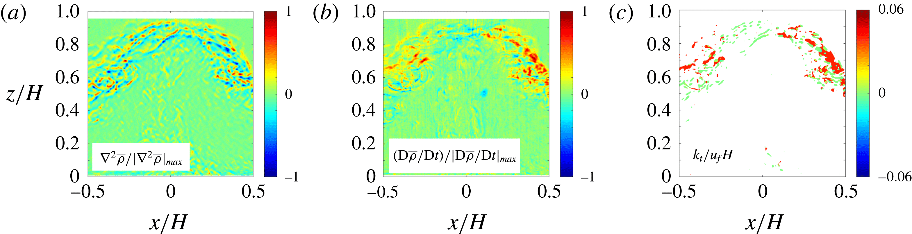
The normalized area
 $a$
identified for this averaging (i.e. cumulative mixing regions at a given time) is shown in figure 12(a), where time moving averaging has been performed with a window of
 $\unicode[STIX]{x0394}tu_{f}/H=1$
for smoothing. It should be noted that
 $a$
consistently achieves its maximum when
 $tu_{f}/H\approx 0$
and decreases quickly thereafter over the collision stage. The time-averaged area
 $A$
was calculated for each case, covering phases I–III
 $(-0.2<tu_{f}/H<2.8)$
. The results are shown in figure 12(b), the error bars being the standard deviations of fluctuations from the moving time average for each ensemble. The average
 $A/H^{2}$
increases with
 $Re$
, assuming an asymptotic value with
 $A/H^{2}\approx 0.037$
if the Reynolds number similarity is achieved (dashed line in figure 12
b), although extension of the
 $Re$
range with a different experimental set-up is required to confirm this claim. Interestingly, the increase and plateauing of
 $A/H^{2}$
is consistent with the mixing transition Reynolds number identified in previous research, where the Reynolds number similarity was identified beyond
 $Re\approx 3000$
(Breidenthal Reference Breidenthal1981).
The cumulative area
 $a$
identified based on patches of realistic eddy diffusivities
 $k_{t}$
in figure 11(c): (a) the time evolution of
 $a/H^{2}$
; (b) the overall time-averaged area
 $A$
over phases I–III. The error bars are the standard deviations of fluctuations from the moving time average.

(a) The time evolution of the dimensionless spatially averaged turbulent diffusivity; (b) the overall space–time-averaged turbulent diffusivity during phases I–III. The error bars are the standard deviations of fluctuations from the moving time average.

Figure 13(a) shows the time evolution of
 $\overline{k_{t}}$
, with moving time averaging conducted as before for
 $a$
. In spite of a somewhat noisy signal, the trends of normalized
 $\overline{k_{t}}$
for all cases are the same. It should be noted that
 $\overline{k_{t}}$
achieves its maximum when the turbulence is strongest and the stratification effects are important
 $(tu_{f}/H\approx 0)$
, as is to be expected, and decreases over the collision stages. The scatter of the curves, however, makes it difficult to delineate a robust decay law. However, for practical purposes, it would be useful to obtain a single eddy diffusivity for mesoscale models, which can be included as a conditional mixing parameterization when a collision is present. To this end, an overall eddy diffusivity
 $K_{T}$
was calculated for each experiment over the entire event. As before, phases I–III
 $(-0.2<tu_{f}/H<2.8)$
were selected for event averaging. The result is shown in figure 13(b). There is a stable trend of
 $K_{T}$
, which appears to be insensitive to
 $Re$
for
 $Re>3000$
. The three high-
 $Re$
cases have a mean value of
 $K_{T}/u_{f}H\approx 3.6\times 10^{-3}$
(dashed line in figure 13
b).
The turbulent Schmidt number can be defined as
 $$\begin{eqnarray}Sc=\frac{K_{T,C4300}}{k}=\frac{4.35\times 10^{-5}}{0.12\times 10^{-9}}=3.63\times 10^{5},\end{eqnarray}$$
where
 $K_{T,C4300}$
is the eddy diffusivity of C4300 and
 $k$
is the molecular diffusivity of salt in water at 300 K. The eddy diffusivity is approximately
 $10^{5}$
times the molecular diffusivity for this case, indicating that turbulent diffusion strikingly dominates mixing for a period
 $-0.2<tu_{f}/H<2.8$
during the collision stage.
7 Discussion
There is an applicability problem in extending the result from laboratory experiments to the atmospheric flows due to huge Reynolds-number differences. The colliding events in the atmosphere have gravity-current length and frontal velocity scales of 100 m and
 $1~\text{m s}^{-1}$
respectively, with a Reynolds number of
 $Re=u_{f}h_{g}/\unicode[STIX]{x1D708}\sim 10^{7}$
. A laboratory lock-exchange tank provides a way to mimic and investigate collisions in a controlled setting, but the highest Reynolds number achievable is (
 $10^{3}$
–
 $10^{5}$
), which is small compared with atmospheric cases. The foundation of the present experimental study is the theoretical notion that turbulent mixing reaches a self-similar stage with a constant eddy diffusivity when
 $Re$
becomes high enough (Barenblatt Reference Barenblatt1996). At this self-similar stage, smaller-scale eddies will dominate mixing without the boundary influence. From figures 12(b) and 13(b), our study appears to enter this self-similar stage when
 $Re>3000$
, a value first proposed by Breidenthal (Reference Breidenthal1981) and discussed by Princevac, Fernando & Whiteman (Reference Princevac, Fernando and Whiteman2005) in the context of atmospheric katabatic flows. Future laboratory and numerical efforts are encouraged to encompass larger Reynolds numbers to validate the applicability of the self-similarity hypothesis.
Some data in this study are relatively scattered, which can be attributed to inherent experimental variability. First, the sample size was relatively small (10 for each case), stoking challenges for convergent turbulence statistics. Experience suggests that hundreds of independent replications are necessary for good statistical convergence, which was impracticable for the present case. The number of trials needed was greater than the number of valid trials due to failure in achieving identical parameters and boundary conditions. This exacerbated the relatively large cost (of 100-proof alcohol,
 ${\sim}20$
L for each realization) associated with an ensemble. To balance competing factors, 10 independent replications were chosen. Second, initial disturbances associated with filling the tank affected the turbulence intensity in gravity currents, as experiments needed to be conducted fairly quickly after filling to prevent evaporation. Third, some quantities such as the turbulence intensity, the turbulent diffusivity and the rate of density change were not directly measured but were derived high-order quantities, for which statistical convergence requires larger sample sizes. To some extent, these problems were alleviated by using phase-aligned ensemble averaging, but a larger sample size is still desired. In spite of data scatter, the trends were clearly evident within experimental error, and thus considerable attention was paid to trends in making inferences. For example, the case C1000 was excluded in vertical front velocity calculations based on the Chauvenet criterion (figure 6) due to its significant deviation from the other cases (figure 5
a). Future experimental and numerical studies should include suitable ensemble sizes and large Reynolds numbers by employing innovative techniques.
The present physical model is a simplified depiction of atmospheric flow collisions, where in the latter the gravity currents are dissimilar in density, velocity and internal structure, are three-dimensional, travel on sloping valleys on rough surfaces within the stable atmospheric boundary layer, collide obliquely and may be affected by the Earth’s Coriolis forces. Thus. our study invites a myriad of future extensions of atmospheric flow collisions.
8 Conclusions
Collision between two counterflowing identical gravity currents was studied using laboratory experiments, with a view to understanding collisions in nature (e.g. between katabatic flows or thunderstorm outflows) and parameterizing associated turbulent mixing for mesoscale models. A two-dimensional lock-exchange configuration was used, with the locks carrying heavier fluid at either end of a long rectangular tank and collisions occurring at the centre. The dense fluid was a saline solution, and an aqueous ethanol having a similar refractive index was used as the lighter ambient fluid. This enabled the use of optical techniques for flow diagnostics. A time-resolved PIV/PLIF system was employed to measure the velocity and density fields simultaneously. The sole governing dimensionless parameter for the problem is the Reynolds number. Ensemble averaging of 10 replications was used with the application of phase alignment to minimize jitter before averaging. Mixing was quantified by tracking the density change of fluid parcels at every point in the flow field. The major findings of the study are as follows.
(i) Collision between two counterflowing gravity currents could be roughly divided into four stages: independent propagation of currents, approach, collision and postcollision slumping (spreading). Most of the turbulence and mixing is generated during the collision stage.
(ii) The length, velocity and time scales during the collision stage were identified respectively as the depth of the fluid
 $H$
, the frontal velocity of the gravity currents
$u_{f}$
and
$H/u_{f}$
.
(iii) The collision stage itself could be divided into three phases, based on the evolution of the density front ensuing the collision. If the time origin is taken as the instant when the (suitably defined) average height of the dense fluid inside a box of size
$H\times H$
(dubbed
$H$
–
$H$
box) equals 0.5
$H$
, phase I occupies from the initial contact of the gravity currents at
$tu_{f}/H=-0.2$
to
$tu_{f}/H=0.5$
. Most of the turbulence in phase I is generated in the proximity of the density interface, but a non-negligible amount of turbulence is also generated within the upper and lower fluids. The average turbulence intensity reaches a maximum at
$tu_{f}/H\approx 0$
. Most of the turbulence production and mixing during the collision occurs in phase I.(iv) Phase II lasts from
$tu_{f}/H\approx 0.5$
to 1.2 and is characterized by a negligible vertical interfacial velocity. An exponential decay law is proposed for phases II and III, wherein turbulence production occurs but is overshadowed by the decay of turbulence.(v) Phase III spans
$1.2<tu_{f}/H<2.8$
, and TKE production therein is negligible. Very little turbulent mixing occurs in phase III, wherein the decay law appears to transition to an algebraic power law.(vi) The strongest turbulent mixing surrounds
$tu_{f}/H\approx 0$
, within isolated patches distributed in the interfacial region between the denser and lighter fluids. The patches occupy a space–time-averaged dimensionless area of
$A/H^{2}\approx 0.037$
at
$Re>3000$
, but show
$Re$
dependence at lower
$Re$
.(vii) The dimensionless eddy diffusivity averaged over the patch area
$\overline{k_{t}}/u_{f}H$
was time-dependent. A representative eddy diffusivity
$K_{T}$
for a collision event could be proposed by averaging
$\overline{k_{t}}$
over phases I–III
$(-0.2<tu_{f}/H<2.8)$
, which could be treated as the lifetime of a collision event. Its normalized value
$K_{T}/u_{f}H$
was dependent on
$Re$
, but for
$Re>3000$
or so this dependence was weak, with
$K_{T}/u_{f}H\approx 3.6\times 10^{-3}$
. This result is recommended as a new conditional parameterization for representing collision events in mesoscale meteorological models.









Acknowledgement
This research was funded by Office of Naval Research Award no. N00014-11-1-0709, Mountain Terrain Atmospheric Modeling and Observations (MATERHORN) Program (2011–2016). During the manuscript preparation and revision phase, the authors were supported by the NSF Grants AGS-1528451 and AGS-1565535 and the College of Water Resources and Civil Engineering, China Agricultural University, Beijing. F.H. was supported by a Mechor Chair Professorship at University of Notre Dame.



