1 Introduction
Air-blast atomization is the process by which a low-speed liquid jet is sheared by a faster gas stream, leading to breakup of the liquid phase into ligaments and small droplets. This phenomenon is ubiquitous in nature, and is of particular interest to the automotive and aerospace industries, as the quality of the combustion, and thus pollutant generation, depends on the characteristics of fuel atomization. In recent years, primary air-blast atomization has been the object of many experimental and theoretical studies (Raynal Reference Raynal1997; Boeck & Zaleski Reference Boeck and Zaleski2005; Eggers & Villermaux Reference Eggers and Villermaux2008; Otto, Rossi & Boeck Reference Otto, Rossi and Boeck2013), where the physics controlling the presence and characteristics of waves has been investigated. Inviscid analysis of primary atomization (Hong, Cartellier & Hopfinger Reference Hong, Cartellier and Hopfinger2002; Marmottant & Villermaux Reference Marmottant and Villermaux2004; Ben Rayana Reference Ben Rayana2007) was carried out and predicted wave frequencies two times smaller than experimental values. Subsequently, Matas, Marty & Cartellier (Reference Matas, Marty and Cartellier2011) obtained fairly good agreement of the frequencies by taking into account during the inviscid analysis the zero interface velocity due to the presence of a splitter plate in the experiments. However, their model predicted a spatial growth rate much lower than that observed in experiments. Using the Orr–Sommerfeld equations, Yecko, Zaleski & Fullana (Reference Yecko, Zaleski and Fullana2002), and later Boeck & Zaleski (Reference Boeck and Zaleski2005), included viscous effects in the temporal linear analysis of the two-phase shear layer and recovered the experimental spatial growth rate, but their predicted frequencies were overestimated.
More recently, Otto et al. (Reference Otto, Rossi and Boeck2013) proposed a spatio-temporal linear theory and obtained reasonably good agreement with experiments for the wave frequencies but an unsatisfactory spatial growth rate. It was also shown in this work that, depending on the experimental parameters, convective or absolute instability can be encountered. This behaviour is clarified and characterized by Fuster et al. (Reference Fuster, Matas, Marty, Popinet, Hoepffner, Cartellier and Zaleski2013), where the transition from convective to absolute instability is shown based on the value of the dynamic pressure ratio,
 $M=\unicode[STIX]{x1D70C}_{g}U_{g}^{2}/\unicode[STIX]{x1D70C}_{l}U_{l}^{2}$
, where
 $\unicode[STIX]{x1D70C}_{g}$
and
 $\unicode[STIX]{x1D70C}_{l}$
are the gas and liquid densities and
 $U_{g}$
and
 $U_{l}$
are the free-stream gas and liquid velocities. Despite the progress in understanding the formation and frequency of liquid waves, the linear theory approach is unsuitable for describing the atomization of liquids in complex geometries or in the presence of turbulence at downstream positions of the injector. Recent experiments (Jerome et al.
Reference Jerome, Marty, Matas, Zaleski and Hoepffner2013) have illustrated the importance of the nonlinear dynamics of the gas stream in the occurrence of droplets catapulted from the crests of liquid waves.
Numerical simulations have become an important asset which can provide some new insights into atomization. However, only a few numerical studies (Bianchi et al. Reference Bianchi, Pelloni, Toninel, Scardovelli, Leboissetier and Zaleski2005; Menard, Tanguy & Berlemont Reference Menard, Tanguy and Berlemont2007; Gorokhovski & Herrmann Reference Gorokhovski and Herrmann2008; Shinjo & Umemura Reference Shinjo and Umemura2010, Reference Shinjo and Umemura2011; Fuster et al. Reference Fuster, Matas, Marty, Popinet, Hoepffner, Cartellier and Zaleski2013) have shown acceptable agreement with experimental observations. This is partly due to the large density ratio and the intense multiscale character of a realistic experimental atomization process (e.g. air/water system). Numerical simulations, in these contexts, are extremely expensive and challenging. This work aims to provide a comparison of numerical simulations with recent experiments on the destabilization of an air-blasted liquid layer and the statistics of the flow.
2 Numerical method
We consider a liquid–gas two-phase flow with constant densities
 $\unicode[STIX]{x1D70C}_{l}$
and
 $\unicode[STIX]{x1D70C}_{g}$
and dynamic viscosities
 $\unicode[STIX]{x1D707}_{l}$
and
 $\unicode[STIX]{x1D707}_{g}$
, the subscripts
 $l$
and
 $g$
referring respectively to the liquid and gas phases. The flow is described by the Navier–Stokes equations in each phase,
 $$\begin{eqnarray}\displaystyle & \displaystyle \unicode[STIX]{x2202}_{t}(\unicode[STIX]{x1D70C}\boldsymbol{u})+\unicode[STIX]{x1D735}\boldsymbol{\cdot }(\unicode[STIX]{x1D70C}\boldsymbol{u}\otimes \boldsymbol{u})=-\unicode[STIX]{x1D735}p+\unicode[STIX]{x1D735}\boldsymbol{\cdot }(2\unicode[STIX]{x1D707}\unicode[STIX]{x1D63F})+\unicode[STIX]{x1D70C}\boldsymbol{g}, & \displaystyle\end{eqnarray}$$
 $$\begin{eqnarray}\displaystyle & \displaystyle \unicode[STIX]{x1D735}\boldsymbol{\cdot }\boldsymbol{u}=0, & \displaystyle\end{eqnarray}$$
where
 $\boldsymbol{u}$
is the fluid velocity,
 $\unicode[STIX]{x1D70C}\equiv \unicode[STIX]{x1D70C}(\boldsymbol{x},t)$
is the density,
 $\unicode[STIX]{x1D707}\equiv \unicode[STIX]{x1D707}(\boldsymbol{x},t)$
is the dynamic viscosity,
 $\unicode[STIX]{x1D63F}$
is the deformation tensor and
 $\boldsymbol{g}$
is the gravitational acceleration. The densities and the viscosities are discontinuous across the interface
 $\unicode[STIX]{x1D6E4}$
separating the two phases. They are represented by their jumps,
 $[\unicode[STIX]{x1D70C}]_{\unicode[STIX]{x1D6E4}}=\unicode[STIX]{x1D70C}_{l}-\unicode[STIX]{x1D70C}_{g}$
and
 $[\unicode[STIX]{x1D707}]_{\unicode[STIX]{x1D6E4}}=\unicode[STIX]{x1D707}_{l}-\unicode[STIX]{x1D707}_{g}$
. The normal stress boundary condition at the interface is expressed by the pressure jump equation,
 $$\begin{eqnarray}\displaystyle [p]_{\unicode[STIX]{x1D6E4}}=\unicode[STIX]{x1D70E}\unicode[STIX]{x1D705}+2[\unicode[STIX]{x1D707}]_{\unicode[STIX]{x1D6E4}}\boldsymbol{n}^{\text{T}}\boldsymbol{\cdot }\unicode[STIX]{x1D735}\boldsymbol{u}\boldsymbol{\cdot }\boldsymbol{n}, & & \displaystyle\end{eqnarray}$$
where
 $\unicode[STIX]{x1D70E}$
is the surface tension coefficient,
 $\unicode[STIX]{x1D705}$
is the curvature of the interface and
 $\boldsymbol{n}$
is the normal vector at the interface. We use an in-house multiphase Navier–Stokes solver (Desjardins et al.
Reference Desjardins, Blanquart, Balarac and Pitsch2008; Owkes & Desjardins Reference Owkes and Desjardins2014, Reference Owkes and Desjardins2015), which discretely conserves mass, momentum and kinetic energy within each phase, although the discontinuity in density across the two-phase interface leads to momentum and kinetic energy conservation errors at the interface. A correction algorithm is employed in order to mitigate these conservation errors. For further details, refer to Desjardins et al. (Reference Desjardins, McCaslin, Owkes and Brady2013). The discontinuous pressure is handled using the ghost fluid method, and the interface between the two phases is tracked and transported based on a semi-Lagrangian geometric volume of fluid (VOF) method (Owkes & Desjardins Reference Owkes and Desjardins2014) coupled with a second-order interface curvature computation based on a height function method (Owkes & Desjardins Reference Owkes and Desjardins2015). Use of the same transport methodology for both the liquid volume fraction and the momentum results in a discretely consistent scheme which provides conservation and second-order accuracy. The consistency of the numerical scheme and the improved discrete conservation of momentum and kinetic energy together with the geometric VOF method make the solver suitable for simulating atomization processes, in which large exchanges of momentum and kinetic energy between the gas and the liquid are likely to arise. For instance, previous two-phase flow simulations of the shear instability presented in Desjardins et al. (Reference Desjardins, McCaslin, Owkes and Brady2013) have shown that the solver is able to predict the most unstable wavenumber well, even on coarse meshes with as few as eight cells per wavelength, corresponding to approximately two cells in the gas boundary layer.
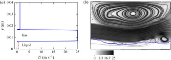
(a) Example of the inflow velocity profile for
 $U_{g}=25~\text{m}~\text{s}^{-1}$
,
 $U_{l}=0.216~\text{m}~\text{s}^{-1}$
and a coflow of 5 %
 $U_{g}$
. The liquid velocity is shown with a dashed red line and the gas velocity with a blue line. A zero velocity is imposed at the splitter plate position between the liquid and the gas. (b) Snapshot of the simulation at
 $tU_{g}/\unicode[STIX]{x1D6FF}_{g}=6400$
, showing the liquid–gas interface, the streamlines and the velocity field.

3 Two-dimensional numerical simulations
We consider the same experimental parameters as in Fuster et al. (Reference Fuster, Matas, Marty, Popinet, Hoepffner, Cartellier and Zaleski2013), shown in their § 2 and table 3. The liquid and the gas are both entering the simulation domain at the left side with heights
 $H_{l}=6.4~\text{mm}$
and
 $H_{g}=10~\text{mm}$
and at different velocities
 $U_{l}$
and
 $U_{g}$
. We account for the splitter plate present in the experiments by imposing a zero velocity in the velocity profile at the splitter plate lip position, as shown in figure 1. The thickness of the lip, denoted by
 $e$
, is set to
 $0.2~\text{mm}$
. The gas inflow is tilted downward with an angle of
 $\unicode[STIX]{x1D6FD}=4.15^{\circ }$
, which corresponds to the experimental splitter plate slope. In the experiment, due to the form of the splitter plate used, such as that in figure 2 of Fuster et al. (Reference Fuster, Matas, Marty, Popinet, Hoepffner, Cartellier and Zaleski2013), the liquid inflow is tilted up with the same angle
 $\unicode[STIX]{x1D6FD}$
. Preliminary simulations have shown no significant difference in the dynamics of the flow when
 $\unicode[STIX]{x1D6FD}$
is accounted for in the liquid inflow velocity; therefore, the inclination
 $\unicode[STIX]{x1D6FD}$
is only applied on the gas phase for this numerical study. We account for entrainment of the gas by adding 5 % of the gas inflow velocity between the gas layer and the upper wall as an additional coflow, as done in da Silva & Métais (Reference da Silva and Métais2002) and Babu & Mahesh (Reference Babu and Mahesh2004). The streamlines of the velocity in the upper gas region are shown in figure 1(b). The gas jet goes down due to the momentum flux difference in the liquid–gas shear layer and is inclined upward at locations further downstream due to the interactions with the liquid waves. This induces a recirculation zone in the upper region, as shown in figure 1(b). The same configuration of the gas inflow entrainment and the recirculation zone is observed in additional simulations (not shown herein) for a coflow of up to 10 % of the gas inflow velocity. The gas boundary layer is computed based on the vorticity thickness
 $\unicode[STIX]{x1D6FF}_{g}/H_{g}=5.2/\sqrt{Re}$
, determined through experimental measurements in Fuster et al. (Reference Fuster, Matas, Marty, Popinet, Hoepffner, Cartellier and Zaleski2013), where the gas Reynolds number is based on the thickness of the gas layer,
 $Re=\unicode[STIX]{x1D70C}_{g}H_{g}U_{g}/\unicode[STIX]{x1D707}_{g}$
. Between the fast gas stream and the coflow, a boundary layer of thickness
 $\unicode[STIX]{x1D6FF}_{g}$
is also prescribed in the inflow velocity field
 $(u,v,0)$
, which is described by the following equations:
 $$\begin{eqnarray}\displaystyle u=\left\{\begin{array}{@{}ll@{}}U_{l}, & 0\leqslant y<H_{l},\\ 0, & H_{l}\leqslant y<H_{l}+e,\\ U_{g}\tanh \left(\!2{\displaystyle \frac{(y-(H_{l}+e))}{\unicode[STIX]{x1D6FF}_{g}}}\!\right) & \\ \quad \times \tanh \left(\!-2{\displaystyle \frac{(y-(H_{l}+e+H_{g}))}{\unicode[STIX]{x1D6FF}_{g}}}\!\right)\cos \left(\unicode[STIX]{x1D6FD}{\displaystyle \frac{\unicode[STIX]{x03C0}}{180}}\right)\!, & H_{l}+e\leqslant y<H_{l}+e+H_{g},\\ 0.05U_{g}\tanh \left(\!2{\displaystyle \frac{(y-(H_{l}+e+Hg))}{\unicode[STIX]{x1D6FF}_{g}}}\!\right), & H_{l}+e+H_{g}\leqslant y\leqslant H,\end{array}\right. & & \displaystyle \nonumber\\ \displaystyle & & \displaystyle\end{eqnarray}$$
 $$\begin{eqnarray}\displaystyle v=\left\{\begin{array}{@{}ll@{}}0, & 0\leqslant y<H_{l}+e,\\ -U_{g}\tanh \left(2{\displaystyle \frac{(y-(H_{l}+e))}{\unicode[STIX]{x1D6FF}_{g}}}\right) & \\ \quad \times \tanh \left(\!-2{\displaystyle \frac{(y-(H_{l}+e+H_{g}))}{\unicode[STIX]{x1D6FF}_{g}}}\!\right)\sin \left(\unicode[STIX]{x1D6FD}{\displaystyle \frac{\unicode[STIX]{x03C0}}{180}}\right), & H_{l}+e\leqslant y<H_{l}+e+H_{g},\\ 0, & H_{l}+e+H_{g}\leqslant y\leqslant H,\end{array}\right. & & \displaystyle \nonumber\\ \displaystyle & & \displaystyle\end{eqnarray}$$
where
 $H$
is the height of the simulation domain.
Since the liquid boundary layer does not play an important role (Ben Rayana Reference Ben Rayana2007; Fuster et al.
Reference Fuster, Matas, Marty, Popinet, Hoepffner, Cartellier and Zaleski2013), its thickness is set to zero at the inlet in the present study. The simulation domain is
 $8H_{l}\times 4.5H_{l}$
in the
 $x$
(streamwise) and
 $y$
(normal) directions respectively, and two different spatial resolutions,
 $\unicode[STIX]{x0394}x=\unicode[STIX]{x1D6FF}_{g}/2,\unicode[STIX]{x1D6FF}_{g}/4$
, corresponding to physical values of
 $195~\unicode[STIX]{x03BC}\text{m}$
and
 $97.5~\unicode[STIX]{x03BC}\text{m}$
, are used. Larger domains with heights of
 $8H_{l}$
and
 $10H_{l}$
have shown no significant difference in the dynamics of the flow. A Dirichlet inflow condition is used as the left boundary condition and a convective outflow with zero normal gradients of the pressure,
 $\unicode[STIX]{x1D735}p\boldsymbol{\cdot }\boldsymbol{n}=0$
(Sani et al.
Reference Sani, Shen, Pironneau and Gresho2006), is used as the right boundary condition. A slip boundary condition is used for both the top and the bottom of the domain.
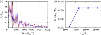
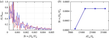
(a) The FFT of the interface height at two different spatial resolutions, in blue for
 $\unicode[STIX]{x1D6E5}_{x}=\unicode[STIX]{x1D6FF}_{g}/2$
and in red for
 $\unicode[STIX]{x1D6E5}_{x}=\unicode[STIX]{x1D6FF}_{g}/4$
. The dashed black line represents the maximum frequency obtained in the experiment (Fuster et al.
Reference Fuster, Matas, Marty, Popinet, Hoepffner, Cartellier and Zaleski2013). (b) Maximum frequency at different time periods. The frequency remains unchanged for a length of time larger than
 $tU_{g}/\unicode[STIX]{x1D6FF}_{g}=18\,300$
.
Simulation parameters.

Simulations with the parameters presented in table 1 are performed in two dimensions (2D) on the two different spatial resolutions mentioned above. The corresponding dynamic pressure ratio is
 $M=16$
for this configuration. The frequency of the waves, expressed as a Strouhal number
 $St=f\unicode[STIX]{x1D6FF}_{g}/U_{g}$
, is extracted by applying a fast Fourier transform (FFT) algorithm to the time evolution of the interface height, recorded at a fixed downstream position
 $x/\unicode[STIX]{x1D6FF}_{g}=25$
, where interface disturbances are small. The necessary sampling time of the signal to obtain an accurate frequency is checked and reported in figure 2(b), where it is shown that the frequency corresponding to the maximum amplitude, hereafter referred to as ‘maximum frequency’, remains unchanged for a time larger than
 $tU_{g}/\unicode[STIX]{x1D6FF}_{g}=18\,300$
, which corresponds to approximately eight formed waves. This length of time is used to compute the FFT presented in this study. Figure 2(a) shows the amplitude of the interface fluctuations as a function of the wave frequencies for two different spatial refinements. The obtained maximum Strouhal number of
 $(4.3\pm 0.25)\times 10^{-4}$
is very close to the corresponding experimental value of
 $5\times 10^{-4}$
presented in Fuster et al. (Reference Fuster, Matas, Marty, Popinet, Hoepffner, Cartellier and Zaleski2013). The result obtained on the finer grid is closer to the experimental value, although both meshes display good agreement with Fuster et al. (Reference Fuster, Matas, Marty, Popinet, Hoepffner, Cartellier and Zaleski2013). The percentage errors relative to the experimental values are shown in table 2. To minimize the computational cost, a uniform cell size of
 $\unicode[STIX]{x0394}x=\unicode[STIX]{x1D6FF}_{g}/2$
is used in the following simulations. The dynamic pressure ratio
 $M$
is changed by varying the liquid entrance velocity
 $U_{l}$
while the gas velocity is kept constant at
 $U_{g}=20~\text{m}~\text{s}^{-1}$
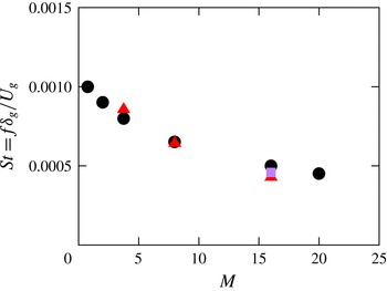
. The accuracy of the computations is confirmed when comparing the maximum frequency obtained at two other values of
 $M$
, namely 3.75 and 8, with the corresponding experimental value. Excellent agreement is obtained, as shown in figure 3.
Comparison of the maximum frequency as a function of
 $M$
obtained from recent experiments (●) (Fuster et al.
Reference Fuster, Matas, Marty, Popinet, Hoepffner, Cartellier and Zaleski2013) for
 $U_{g}=20~\text{m}~\text{s}^{-1}$
and
 $M=16$
and the present 2D simulations (red ▵). The symbol ▫ at
 $M=16$
corresponds to the maximum frequency extracted from the three-dimensional simulation presented later in this paper.

Accuracy of the maximum frequency obtained from numerical simulations at two different mesh resolutions.

The thickness of the separator plate lip has been shown to have an impact on the most unstable frequency. Indeed, a splitter plate thickness larger than the gas boundary layer decreases the maximum frequency (Ben Rayana Reference Ben Rayana2007; Fuster et al.
Reference Fuster, Matas, Marty, Popinet, Hoepffner, Cartellier and Zaleski2013). However, the influence of the separator plate slope has not been investigated previously. In order to explore the role played by the slope
 $\unicode[STIX]{x1D6FD}$
, simulations are performed at
 $M=16$
with four different values of
 $\unicode[STIX]{x1D6FD}$
between
 $0^{\circ }$
and
 $30^{\circ }$
. As previously mentioned, the slope of the separator plate is taken into account by introducing a downward inclination of equivalent angle on the gas inflow.
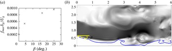
Influence of the slope
 $\unicode[STIX]{x1D6FD}$
of the gas inflow on the flow dynamics for
 $U_{g}=20~\text{m}~\text{s}^{-1}$
and
 $M=16$
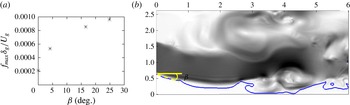
. (a) Maximum frequency plotted as a function of
 $\unicode[STIX]{x1D6FD}$
. (b) Example of an initially flat liquid layer matching the gas stream inclination of
 $25^{\circ }$
. The labels are in cm.
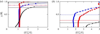
Mean liquid velocity (a) close to the domain entrance
 $x/H_{l}=0.9$
and (b) at a far-field position
 $x/H_{l}=6$
, for
 $\unicode[STIX]{x1D6FD}=0^{\circ }$
(red ○),
 $\unicode[STIX]{x1D6FD}=4.15^{\circ }$
(blue ▫) and
 $\unicode[STIX]{x1D6FD}=16.6^{\circ }$
(black ▵), and for
 $U_{g}=20~\text{m}~\text{s}^{-1}$
and
 $M=16$
. The horizontal dashed lines show the interface positions (represented by the ordinate of the point corresponding to the 0.5 VOF iso-surface). The mean liquid velocity is defined by
 $\langle U\rangle _{t}^{l}=(\langle \unicode[STIX]{x1D6FC}(\boldsymbol{x},t)U(\boldsymbol{x},t)\rangle _{t})/(\langle \unicode[STIX]{x1D6FC}(\boldsymbol{x},t)\rangle _{t})$
, where
 $\unicode[STIX]{x1D6FC}(\boldsymbol{x},t)$
is the volume fraction of the liquid phase, with
 $\boldsymbol{x}$
as the position and
 $t$
as time (
 $\langle \cdot \rangle _{t}$
represents the time average).

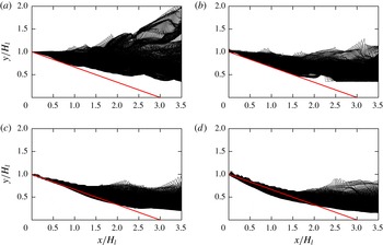
Liquid cone length for different gas inflow inclinations for
 $U_{g}=20~\text{m}~\text{s}^{-1}$
and
 $M=16$
: (a)
 $\unicode[STIX]{x1D6FD}=0^{\circ }$
, (b)
 $\unicode[STIX]{x1D6FD}=4.15^{\circ }$
, (c)
 $\unicode[STIX]{x1D6FD}=16.6^{\circ }$
and (d)
 $\unicode[STIX]{x1D6FD}=25^{\circ }$
. The red line represents the correlation length of (3.3).

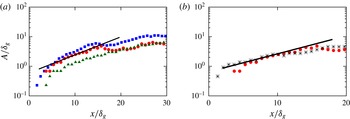
(a) Spatial growth rate for different values of
 $\unicode[STIX]{x1D6FD}$
,
 $0^{\circ }$
(blue ▫),
 $4.15^{\circ }$
(red ○) and
 $25^{\circ }$
(dark green ▵), and (b) spatial growth rate at two different resolutions,
 $\unicode[STIX]{x0394}x=\unicode[STIX]{x1D6FF}_{g}/2$
(red ○) and
 $\unicode[STIX]{x0394}x=\unicode[STIX]{x1D6FF}_{g}/4$
(black
 $\ast$
), for
 $U_{g}=20~\text{m}~\text{s}^{-1}$
and
 $M=16$
. The black line represents the exponential fit,
 $0.6\exp (0.14x/\unicode[STIX]{x1D6FF}_{g})$
, corresponding to a spatial growth rate of
 $k\unicode[STIX]{x1D6FF}_{g}=0.14$
.

The wavy structure appearing on the liquid interface has been thought to arise from a Kelvin–Helmholtz instability of the mixing layer (Marmottant & Villermaux Reference Marmottant and Villermaux2004; Ben Rayana, Cartellier & Hopfinger Reference Ben Rayana, Cartellier and Hopfinger2006). Moreover, it is well known that the tilt angle has a destabilizing effect on a Kelvin–Helmholtz-like perturbation, as discussed in Negretti, Socolofsky & Jirka (Reference Negretti, Socolofsky and Jirka2008). In our simulations, the initially flat liquid layer becomes parallel to the fast gas stream close to the domain entrance after a few time steps, as shown in figure 4(b). Then, the shear between the liquid and the gas takes place in an inclined configuration, as seen in figure 5, which adds an additional acceleration to the interface in the upstream region. Consequently, increase of the slope
 $\unicode[STIX]{x1D6FD}$
enhances the formation of liquid waves. Indeed, the maximum frequency of the waves increases monotonically with
 $\unicode[STIX]{x1D6FD}$
, as shown in figure 4(a). Figure 6, where the instantaneous liquid interface is superimposed over a 0.4 s interval, shows the potentially formed liquid cone for four different slopes
 $\unicode[STIX]{x1D6FD}$
at a fixed dynamic pressure of
 $M=16$
. The length of the liquid cone, formed due to the penetration and the entrainment of the liquid by the fast gas flow, is compared with the experimental correlation length proposed by Raynal (Reference Raynal1997),
 $$\begin{eqnarray}\displaystyle L_{\mathit{cone}}/H_{l}=12/M^{0.5}. & & \displaystyle\end{eqnarray}$$
Good agreement is obtained for lower values of
 $\unicode[STIX]{x1D6FD}$
, with the interface in figure 6(a,b) close to the red line. However, the length of the cone is shorter than the experimental correlation when
 $\unicode[STIX]{x1D6FD}$
is large, as in figure 6(c,d). The calculation of the spatial growth rate is performed using the methodology described in Matas et al. (Reference Matas, Marty and Cartellier2011). The amplitude in figure 7 is computed by measuring the width of the histogram of the interface positions at different downstream positions over eight periods of the instability wave. Figure 7(a) shows the downstream evolution of the amplitude for three different values of
 $\unicode[STIX]{x1D6FD}$
, namely
 $0^{\circ }$
,
 $4.15^{\circ }$
and
 $25^{\circ }$
. For the set of parameters used, one can deduce, based on figures 19(b) and 20(b) of Matas et al. (Reference Matas, Marty and Cartellier2011), an exponential evolution of the amplitude at downstream positions
 $x/\unicode[STIX]{x1D6FF}_{g}$
between 2 and 12, with spatial growth rates between 0.1 and 0.17. The exponential fit in figure 7 shows a spatial growth rate of 0.14, which agrees well with the experimental correlation. It should be noted that a direct comparison is not possible due to the difference in liquid velocities used. Nonetheless, the exponential growth is observed at positions further downstream compared with the experiment. This is believed to be due to the fact that for low amplitudes, such as those near the inlet, the change in height will be poorly resolved. This can lead to perceived, faster than exponential, growths as the amplitude grows large enough to be adequately resolved by the computational mesh. Indeed, better results are obtained on the finer grid, with the exponential spatial growth rate appearing earlier in figure 7(b). It should be noted that, while this super-exponential growth rate near the inlet in our simulations has been attributed to a lack of resolution, it has also been observed experimentally, and can be seen in figure 19(b) of Matas et al. (Reference Matas, Marty and Cartellier2011). As shown in figure 7(a), the amplitude decreases with
 $\unicode[STIX]{x1D6FD}$
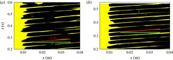
while the obtained spatial growth rate remains unchanged. Furthermore, figure 8 presents a global spatio-temporal view of the liquid wave dynamics by using a Hovmöller diagram, as recently used in Odier et al. (Reference Odier, Balarac, Corre and Moureauc2015) to characterize the convective speed of a flapping liquid sheet. The diagram is constructed by examining the streamwise distribution of liquid and gas along the line
 $y_{0}=0.6H_{l}$
. Fractions of that line in the liquid phase are represented in yellow in the figure, while the gas phase is shown in black. The slope of these lines, the horizontal distance and the vertical distance between two successive lines correspond to the inverse of the convective velocity, the wavelength and the period of the waves respectively. The convective velocity of the waves and the wavelength in figure 8(a,b) agree very well with the expected wave speed (Dimotakis Reference Dimotakis1986)
 $U_{c}=(\sqrt{\unicode[STIX]{x1D70C}_{l}}U_{l}+\sqrt{\unicode[STIX]{x1D70C}_{g}}U_{g})/(\sqrt{\unicode[STIX]{x1D70C}_{l}}+\sqrt{\unicode[STIX]{x1D70C}_{g}})=0.837~\text{m}~\text{s}^{-1}$
and the axial wavelength (Ben Rayana Reference Ben Rayana2007)
 $\unicode[STIX]{x1D706}=1.6\sqrt{\unicode[STIX]{x1D70C}_{l}/\unicode[STIX]{x1D70C}_{g}}\unicode[STIX]{x1D6FF}_{g}=0.02~\text{m}$
. The convective velocity remains unchanged when increasing the inflow velocity inclination
 $\unicode[STIX]{x1D6FD}$
, as shown in figure 8(b). However, the liquid interface becomes increasingly unstable, resulting in the formation of additional waves.
Hovmöller diagrams showing the spatio-temporal evolution of the liquid waves for
 $U_{g}=20~\text{m}~\text{s}^{-1}$
and
 $M=16$
. The red segment is plotted with a slope equal to the inverse of the convective velocity of the waves
 $U_{c}$
(Dimotakis Reference Dimotakis1986) and the green segment has a length equal to the wavelength
 $\unicode[STIX]{x1D706}$
(Ben Rayana Reference Ben Rayana2007): (a)
 $\unicode[STIX]{x1D6FD}=4.15^{\circ }$
, (b)
 $\unicode[STIX]{x1D6FD}=16.6^{\circ }$
.

4 Three-dimensional numerical simulation
A full three-dimensional (3D) simulation is performed next in order to explore the statistics of the flow. A domain of size
 $8H_{l}\times 10H_{l}\times 3H_{l}$
in the
 $x\times y\times z$
(spanwise) directions is used, along with the same physical properties as presented in table 1 with
 $U_{g}=25~\text{m}~\text{s}^{-1}$
,
 $M=16$
and a coflow of 10 %. Direct numerical simulations of such complex three-dimensional two-phase flows at these experimental density and velocity ratios are extremely expensive and so far have not been reported in the literature. In fact, recent studies, such as that of Jerome et al. (Reference Jerome, Marty, Matas, Zaleski and Hoepffner2013), have concluded that such simulations are currently not feasible. The present study is a step towards filling this gap, with a large-eddy simulation (LES), where we resolve large-scale flow features and model the effect of subfilter fluctuations on resolved scales using a subgrid scale (SGS) model. The spatial resolution used for the simulation corresponds to
 $\unicode[STIX]{x0394}x=\unicode[STIX]{x1D6FF}_{g}/2=195~\unicode[STIX]{x03BC}\text{m}$
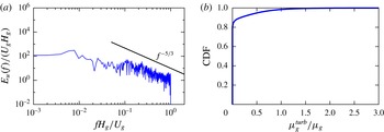
, which was shown in the above 2D simulations to be sufficient to capture the streamwise wave dynamics. In the context of the SGS model used, the Lagrangian dynamic SGS model of Meneveau, Lund & Cabot (Reference Meneveau, Lund and Cabot1996), subfilter interfacial corrugations are simply neglected. Additionally, the effects of filtering variables across the liquid–gas interface are similarly ignored, as further explained in Desjardins et al. (Reference Desjardins, McCaslin, Owkes and Brady2013). The temporal spectrum of the streamwise velocity, shown in figure 9(a), exhibits a well-defined slope close to
 $-5/3$
which extends over approximately one decade. The SGS model itself has limited impact on the majority of the domain since approximately 90 % of cells show only a 10 % or less change to viscosity due to the SGS model, as shown in figure 9(b).
At this resolution, small interface features and microscale physics, such as rim dynamics and the pulling of thin ligaments from wave crests, will not be captured; therefore, the downstream atomization process might not be accurately represented. However, the maximum streamwise wave frequency for the 3D simulation is in agreement with the 2D simulation and the experiment, as shown in figure 3. The simulation was run over three months in parallel on 240 cores to reach the same dimensionless time of 18 300 as used for the FFT in the previously presented 2D simulations.
(a) Temporal spectrum of the streamwise gas velocity at
 $x/H_{l}=7$
and
 $y/H_{l}=2.5$
. (b) Cumulative distribution function (CDF) of the turbulent viscosity ratio in the gas.

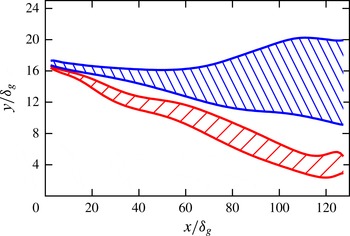
Two characteristic mixing regions around the liquid interface are extracted and are shown in figure 10. The mixing layer thickness is computed based on the average, in both time and the spanwise
 $z$
direction, VOF field (
 $\unicode[STIX]{x1D6FF}_{VOF}$
) and the streamwise velocity profile around the interface (
 $\unicode[STIX]{x1D6FF}_{U}$
). The VOF field
 $\unicode[STIX]{x1D6FF}_{VOF}$
is computed at each
 $x$
location by calculating the vertical distance between the ordinate of the point corresponding to the 0.5 VOF iso-surface and the intersection of the tangent to the average VOF profile at the position (
 $x$
,
 $y_{VOF|_{0.5}}$
) with the
 $y$
-axis
 $y_{T}$
,
 $\unicode[STIX]{x1D6FF}_{VOF}=|y_{VOF|_{0.5}}-y_{T}|$
. Figure 10 shows
 $y_{VOF|_{0.5}}$
as a function of downstream position, with a hatched region corresponding to the mixing layer thickness around
 $y_{VOF|_{0.5}}$
. The VOF-based mixing layer is used to describe the region where liquid and gas mix. A velocity-based mixing layer is obtained using a similar treatment on the streamwise velocity using the point corresponding to half of the maximum velocity, identifying the shear-dominated region. It should be noted that only velocity averages of points with ordinates smaller than
 $y_{\langle U\rangle _{t,z|max}^{g}}$
are considered in the velocity mixing layer computation. As shown in figure 10, the thickness of the velocity-based mixing layer rises faster with the downstream position compared with the VOF-based mixing layer. Figure 10 also shows that the velocity-based layer is located above the VOF-based layer at all downstream positions. This suggests that the region of highest shear and the average interface location rapidly become spatially segregated as the flow evolves downstream, indicating that turbulence–interface interactions happen mostly when breaking waves and ligaments formed at wave crests are pulled up in the high-shear gas region, well above the mean interface location.
Downstream evolution of the velocity-based layer (top blue hatched area) and the VOF-based layer (bottom red hatched area).

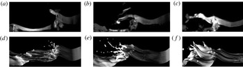
Time sequences, (a–c) and (d–f), of the liquid–gas interface with a 30 ms interval between images. (a–c) Experimental images obtained from the supplementary material of Jerome et al. (Reference Jerome, Marty, Matas, Zaleski and Hoepffner2013). (d–f) Present simulation snapshots.

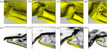
Figure 11 shows a time sequence of the liquid interface, with a 30 ms interval between the images. The images shown in figure 11(a–c) correspond to the interface visualization in the experiment, captured by adding fluorescein to the liquid phase, with the images obtained from the supplementary material of Jerome et al. (Reference Jerome, Marty, Matas, Zaleski and Hoepffner2013), while the images shown in figure 11(d–f) are obtained from the present simulation. Fairly good qualitative agreement of the longitudinal formation of the liquid wave, followed by the ligament and sheet formation at the wave crest and its subsequent flapping, is observed. However, the sheets at the wave crest in the simulation are biased towards ligaments due to limited resolution of the sheets. It is expected that higher resolution would lead to the capturing of thinner ligaments, eventually approaching the thin sheets seen experimentally. Moreover, spanwise undulations of the interface are more prevalent in the simulation snapshots than in the experiments. We believe that this could be due to the particular lighting set-up used to obtain the experimental images, where emphasis was put on capturing the longitudinal waves. In other images generated at the same experimental facility, such as figure 3 of Fuster et al. (Reference Fuster, Matas, Marty, Popinet, Hoepffner, Cartellier and Zaleski2013) and movie 1 of the supplementary material of Jerome et al. (Reference Jerome, Marty, Matas, Zaleski and Hoepffner2013), spanwise waves are clearly evident. Figure 12 depicts a droplet catapult mechanism previously described by Jerome et al. (Reference Jerome, Marty, Matas, Zaleski and Hoepffner2013). A recirculation zone first appears in the wake of the wave. Subsequently, the wave crest is stretched and forms a thin liquid film; this film oscillates and eventually breaks into droplets due to vortex separation and shedding in the gas. While following the mechanism discussed in Jerome et al. (Reference Jerome, Marty, Matas, Zaleski and Hoepffner2013), we believe that the simulation resolution leads to premature breakup, preventing ligaments and droplets as small as those seen experimentally.
Time sequence of wave dynamics by zooming in on the interface (a–d) and the corresponding 2D side view (e–h) of the interface and the vorticity magnitude. (a–d) and (e–h)
 $t=0.371~\text{s}$
, 0.378 s, 0.380 s, 0.384 s.

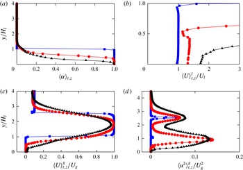
(a) Mean liquid phase volume fraction, (b) mean liquid velocity and (c) mean gas velocity at three different downstream positions:
 $x/H_{l}=0.1$
(blue ▫),
 $x/H_{l}=4$
(red ○) and
 $x/H_{l}=6$
(black ▵). The average is computed both in time
 $t$
and in the
 $z$
direction. (d) Variance of the gas velocity fluctuations.

The statistics of the flow are analysed by averaging both in time
 $t$
and in the
 $z$
direction, hereafter denoted by
 $\langle \cdot \rangle _{t,z}$
. The averages of the liquid and gas phase velocities, respectively
 $\langle U\rangle _{t,z}^{l}$
and
 $\langle U\rangle _{t,z}^{g}$
, are computed as follows:
 $$\begin{eqnarray}\displaystyle \langle U(\boldsymbol{x},t)\rangle _{t,z}^{l}=\frac{\langle \unicode[STIX]{x1D6FC}(\boldsymbol{x},t)U(\boldsymbol{x},t)\rangle _{t,z}}{\langle \unicode[STIX]{x1D6FC}(\boldsymbol{x},t)\rangle _{t,z}} & & \displaystyle\end{eqnarray}$$
and
 $$\begin{eqnarray}\displaystyle \langle U(\boldsymbol{x},t)\rangle _{t,z}^{g}=\frac{\langle (1-\unicode[STIX]{x1D6FC}(\boldsymbol{x},t))U(\boldsymbol{x},t)\rangle _{t,z}}{\langle (1-\unicode[STIX]{x1D6FC}(\boldsymbol{x},t))\rangle _{t,z}}, & & \displaystyle\end{eqnarray}$$
where
 $\unicode[STIX]{x1D6FC}(\boldsymbol{x},t)$
is the volume fraction of the liquid phase, with
 $\boldsymbol{x}$
as the position and
 $t$
as time. The statistics were averaged over the same length of time as the height data were captured for in the FFT, 0.4 s. The mean liquid phase volume fraction, the mean gas velocity and the mean liquid velocity are shown in figure 13 at three different locations in the streamwise direction,
 $x/H_{l}=0.1$
,
 $x/H_{l}=4$
and
 $x/H_{l}=6$
. The mean liquid phase decreases at downstream positions, as seen in figure 13(a), due to the formation of the liquid cone. The liquid sheet is accelerated downstream by the gas and creates a liquid shear layer, as shown in figure 13(b). Figure 13(c) presents a smoothing of the average gas velocity and an increasing gas shear layer thickness with the downstream position. The computed average of the velocity field is then used to obtain the velocity fluctuation
 $u(\boldsymbol{x},t)$
, with figure 13(d) showing the variance of the gas velocity fluctuation
 $\langle u^{2}(\boldsymbol{x},t)\rangle _{t,z}^{g}$
. The gas stream appears to be turbulent at both the upper, gas–gas, and lower, liquid–gas, shear layers. The transition to turbulence in the lower shear layer appears at positions further downstream compared with the upper shear layer, shown by the difference between the blue and red curves in figure 13(d).
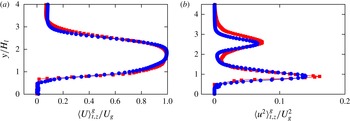
Comparison of the gas phase statistics in 2D (red ▫) and 3D (blue ○) simulations at the downstream position
 $x/H_{l}=4$
. (a) Mean gas velocity and (b) variance of the gas velocity fluctuations.

The gas phase velocity average and fluctuation profiles are compared with those obtained in the corresponding time average two-dimensional simulation. As shown in figure 14, no significant difference can be seen in the average gas velocity, as expected since the flow is largely governed by 2D dynamics. The gas velocity fluctuations, on the other hand, exhibit significant differences.
5 Conclusion
Numerical simulations studying the initial destabilization of an air-blasted liquid layer have been performed for different identified regimes of instability. Excellent agreement of the liquid cone length, maximum wave frequency and spatial growth rate of the interface disturbance is obtained when comparing with experiments. The inclination of the gas inflow is shown to enhance the formation of the liquid waves. The three-dimensional simulation, run using physically correct air/water parameters, shows the formation and flapping of a sheet at the crest of the liquid waves. The sheet subsequently breaks into droplets and liquid fragments, as Jerome et al. (Reference Jerome, Marty, Matas, Zaleski and Hoepffner2013) recently observed in experiments. The statistical analysis of the flow shows an acceleration of the liquid phase and the formation and growth of a liquid boundary layer. The gas stream is found to be turbulent in both the upper gas–gas and lower liquid–gas shear layers. Mixing layers based on the velocity and the VOF fields are computed and show that the mean interface location rapidly becomes segregated from the shear-dominated region in the gas. A comparison of the gas phase statistics between the two-dimensional and three-dimensional computations shows no significant difference for the average streamwise velocity, probably due to the strong 2D nature of the wave dynamics.
The breakup into droplets is of particular interest as it determines the droplet size distribution, which is important for industrial applications. However, substantially more resolution will be required for an exhaustive study of the thin sheet breakup in three-dimensional simulations. Furthermore, the current three-dimensional simulations are prohibitively expensive for the performance of parametric studies, making it impossible to adequately characterize the role of the splitter plate angle and thickness, as well as the momentum ratio, in the true three-dimensional flow configuration. To remedy this, more efficient interface tracking schemes are needed.
Acknowledgements
The authors thank the National Science Foundation for support through grant no. 1351545 and B. M. Lowe for valuable discussions.