



1. Introduction
Microswimmers navigating in a confined environment have a plethora of biological phenomena and engineering applications. These include leukocytes migrating through blood vessels (Kohutek & Bystricky Reference Kohutek and Bystricky2019; Kameritsch & Renkawitz Reference Kameritsch and Renkawitz2020), Escherichia coli bacteria residing in tissue surface folds (Seymour et al. Reference Seymour, Brumley, Stocker and Raina2024; Torres et al. Reference Torres, Pradeep, Ran, Jerolmack and Arratia2024) and various microbial communities inhabiting soil crevices (Donaldson, Lee & Mazmanian Reference Donaldson, Lee and Mazmanian2015; Karita, Limmer & Hallatschek Reference Karita, Limmer and Hallatschek2022). Additionally, micro-squirmers exhibit excellent biocompatibility and swimming efficiency, attracting significant interest in artificial micro-nanorobots for targeted drug delivery within bodily microchannels (Wang et al. Reference Wang, Duan, Ahmed, Sen and Mallouk2015). A comprehensive understanding of micro-swimmer locomotion strategies and the associated hydrodynamic mechanisms in confined spaces is crucial for advancements in gene therapy (Brody Reference Brody2018), biomimetic applications (Yan et al. Reference Yan2017), drug delivery (Guzmán & Maestro Reference Guzmán and Maestro2022) and the development of efficient micro-nano swimming cargo carriers (Li et al. Reference Li, Qin, Gopinath, Arratia, Thomases and Guy2017; Soto et al. Reference Soto, Wang, Ahmed and Demirci2020). Hence, the cargo carrying by swimmers is significant research in the field of targeted drug delivery.
The locomotion and migration behaviours of microswimmers exhibit a plethora of intriguing phenomena (Lauga & Powers Reference Lauga and Powers2009; Ishikawa Reference Ishikawa2023), which have garnered significant academic interest in nutrient transport (Michelin & Lauga Reference Michelin and Lauga2013; Pöhnl, Popescu & Uspal Reference Pöhnl, Popescu and Uspal2019; Wadhwa & Berg Reference Wadhwa and Berg2021), the erratic dances of algae (Pedley, Brumley & Goldstein Reference Pedley, Brumley and Goldstein2016; Ishikawa et al. Reference Ishikawa, Pedley, Drescher and Goldstein2020), autonomous navigation (Qiu et al. Reference Qiu, Mousavi, Gustavsson, Xu, Mehlig and Zhao2021; Sankaewtong et al. Reference Sankaewtong, Molina, Turner and Yamamoto2023, Reference Sankaewtong, Molina and Yamamoto2024), biofilm formation (Li & Ardekani Reference Li and Ardekani2014; Van Wolferen, Orell & Albers Reference Van Wolferen, Orell and Albers2018), bacterial random motility (Howse et al. Reference Howse, Jones, Ryan, Gough, Vafabakhsh and Goldestanian2007; Raza et al. Reference Raza, George, Kumari, Mitra and Paul2023) and sperm cell motility (Friedrich & Julicher Reference Friedrich and Julicher2009; Nassir, Levi & Shaked Reference Nassir, Levi and Shaked2023). The classical ‘squirmer model’ introduced by Lighthill (Reference Lighthill1952) and later extended by Blake (Reference Blake1971) has now been extensively applied to investigate the motion behaviour of pullers, pushers and neutral swimmers in complex geometries and fluid environments (Wu, Hsiao & Woon Reference Wu, Hsiao and Woon2018). For instance, Ishikawa & Hota (Reference Ishikawa and Hota2006) investigated the hydrodynamic interactions between two squirmers and noted their mutual repulsion and rotational movement. Qi et al. (Reference Qi, Annepu, Gompper and Winker2020) found the motion of spheroidal squirmers in microchannel flow was significantly affected by their aspect ratio, prolate spheroids were more likely to rotate with the helical or oscillatory upstream motion, while oblate spheroids exhibited the stable orientation. Nie et al. (Reference Nie, Ying, Guan, Lin and Ouyang2023) simulated the settling of two squirmers in a vertical channel under gravity, identifying three motion patterns: stable descent, stable tilt and oscillatory movements of varying scales. Lauga et al. (Reference Lauga and Powers2023) and Théry et al. (Reference Théry, Maaß and Lauga2023) also studied the sedimentation of squirmers in confined channels and found that the mediated interactions between the wall boundary and the squirmers led to the formation of clusters, which were not found in the bulk fluid. Li & Ardekani (Reference Li and Ardekani2014) found that puller and pusher showed a stronger tendency towards wall-directed motion than a neutral swimmer. However, those works neglect the chiral effect of a microswimmer. Many chiral microswimmers often exhibit spinning motion, moving along helical paths, resulting in asymmetric propulsion and the generation of an asymmetric flow field (Fauci & Dillon Reference Fauci and Dillon2006; Friedrich & Jülicher Reference Friedrich and Jülicher2007; Jékely et al. Reference Jékely, Colombelli, Hausen, Guy, Stelzer, Nédelec and Arendt2008; Burada, Maity & Jülicher Reference Burada, Maity and Jülicher2022). Consequently, the locomotion of a chiral microswimmer gives rise to many different behaviours (Carenza et al. Reference Carena, Gonnella, Marenduzzo and Negro2019; Lancia et al. Reference Lancia, Yamamoto, Ryabchun, Yamaguchi, Sano and Katsonis2019; Yamamoto & Sano Reference Yamamoto and Sano2019). For instance, chiral bacteria with tufted flagella (e.g. E. coli, Bacillus anthracis) exhibit ‘wobble’ trajectories during locomotion (Darnton et al. Reference Darnton, Turner, Rojevsky and Berg2006; Hyon et al. Reference Hyon, Marcos, Powers, Stocker and Fu2012), which are considered two-dimensional projections of their helical movement in three-dimensional space. Park et al. (Reference Park, Kim and Lim2019a) found that single-flagellated bacteria (e.g. Acidobacterium, Oligotropha) reached the target position by reversing the rotational direction of their flagellar motor. They further developed a chiral model of microswimmers with tailed flagella, quantifying the effects of flagellar geometry on swimming velocity and circular radius, and noting that the longer flagella resulted in smaller circular radii (Park, Kim & Lim Reference Park, Kim and Lim2019b). Samatas & Lintuvuori (Reference Samatas and Lintuvuori2023) studied the synchronisation of trajectories of spherical microswimmers with chiral paths in suspension, demonstrating that the hydrodynamic synchronisation was a natural collective behaviour for chiral microswimmers.
The locomotion mechanisms of individual squirmers have been largely studied, however, there is relatively little research on the movement of combined squirmer systems or the swimmer dumbbell, which is considered as the minimal model for connecting microswimmers. To understand the swimming behaviour is crucial for constructing large microswimmer populations, such as autonomous micro-robots (Ishikawa Reference Ishikawa2019) and new functional soft materials (Cates & MacKintosh Reference Cates and Mackintosh2011; Winkler & Gompper Reference Winkler and Gompper2020). The swimmer dumbbell consists of two equal or unequal spheres that can oscillate or rotate, typically connected or constrained in space by rods. Clopés, Gompper & Winkler (Reference Clopés, Gompper and Winkler2020) studied the swimming behaviour of a rod swimmer dumbbell and found that a pair of pullers exhibited a swimming speed significantly lower than a pair of pushers. Ouyang & Lin (Reference Ouyang and Lin2021) found that the swimming velocity of a swimming rod in a Newtonian fluid was significantly influenced by fluid inertia, the swimming mode and the spacing between adjacent rods. This swimmer dumbbell has been partially studied through simulations and experiments (Putz & Dunkel Reference Putz and Dunkel2010; Collis, Chakraborty & Sader Reference Collis, Chakraborty and Sader2017; Dombrowski, Nguyen & Klotsa Reference Dombrowski, Nguyen and Klotsa2022). For example, Ishikawa (Reference Ishikawa2019) created three distinct rod dumbbell models with various connection methods and utilised linear stability analysis to investigate the stability of dumbbell swimmers, uncovering an intrinsic relationship between stability mechanisms and the torque balance of the swimmers. In the aforementioned studies, swimmers were interconnected via a rigid rod, ensuring a fixed inter-swimmer distance. This configuration suggests that the locomotion of dumbbell models is restricted by the internal degrees of freedom, rendering the microswimmer’s motion behaviour insensitive to the environment. (Ziegler et al. Reference Ziegler, Hubert, Vandewalle, Harting and Smith2019). In reality, recent research indicated that the changes of particle spacing were crucial for the movement of the swimmer dumbbell, such as providing the optimal driving frequency in overdamped states (Sukhov et al. Reference Sukhov, Ziegler, Xie, Trosman, Pande, Grosjean, Hubert, Vandewalle, Smith and Harting2019), promoting propulsion by enhancing hydrodynamic interactions (Pande & Smith Reference Pande and Smith2015) and being a key factor in maximising the swimming velocity (Zhou et al. Reference Zhou, Wu, Wu, Jia and Tsui2017).
In scenarios where microswimmers are engaged in tasks such as predation, transportation and targeted drug delivery (Wang et al. Reference Wang, Duan, Ahmed, Sen and Mallouk2015; Bazzi et al. Reference Bazzi, Shammas, Asmar and Mason2017; Jin et al. Reference Jin, Chen and Maass2021), the cargo or passive particles may require another microswimmer to assume the associated locomotive load. Ouyang et al. (Reference Ouyang, Lin, Lin, Yu and Phan-Thien2023) investigated the motion behaviour of non-chiral cargo swimmers with fixed spacing in a Newtonian fluid, they found that the pusher–cargo model exhibited significantly higher swimming speeds than the other models. Debnath & Ghosh (Reference Debnath and Ghosh2018) also discovered that cargo-carrying Janus particles with fixed spacing could significantly enhance their escape from local low-energy traps under flow conditions, with the cargo-carrying capacity depended on the self-propulsion speed of the Janus particles. Yamamoto et al. (Reference Yan2024) integrated a deep reinforcement learning framework to achieve optimal navigation of a cargo-towing swimmer under zig-zag flow conditions. Conversely, some studies rely on some manmade spinning particles for cargo transportation. For example, Gutman & Or (Reference Gutman and Or2016) investigated magnetic microswimmers with flexible tail rotation for optimal cargo-carrying velocity, determining the tail length for maximum velocity. Pak et al. (Reference Pak, Zhu, Brandt and Lauga2012) and Puente et al. (Reference Puente, Godínez, Lauga and Zenit2019) found that the dumbbell model composed of two unequal size manmade spheres with fixed spacing could propel itself in a viscoelastic fluid through tail spin, with the propulsive force arising from the strong viscoelastic jets emitted from the tail, enabling cargo propulsion. Binagia & Shaqfeh (Reference Binagia and Shaqfeh2021) further extended this concept to include any freely suspended spinning body or multiple tail structures. Kroo et al. (Reference Kroo, Binagia, Eckman, Prakash and Shaqfeh2022) optimised the tail geometry of dumbbell models by using shadow imaging to achieve the maximum cargo-carrying velocity. The above research mainly focuses on the cargo-carrying velocity of passive manmade or magnetic particles, there are more applications when the cargo is carried by chiral swimmers in numerous biological and engineering applications, but existing research is insufficient. For instance, magnetically manipulated magnetotactic E. coli can be targeted for localisation and multi-stimuli responsive drug release (Zhang et al. Reference Zhang, Li, Gao, Fan, Pang, Li, Wu, Xie and He2021; Akolpoglu et al. Reference Akolpoglu, Alapan, Dogan, Baltaci, Yasa, Tural and Sitti2022). Additionally, ‘spermbots’ helically structured devices, can capture, guide and release single sperm cells for assisted fertilisation by using external magnetic fields (Magdanz et al. Reference Magdanz, Medina-Sánchez, Schwarz, Xu, Elgeti and Schmidt2017).
The aforementioned studies have shed light on several overlooked aspects: the insufficient research on the influence of elastic degrees of freedom in dumbbell models, neglecting the coupling between chiral and non-chiral propulsion, and there is no research on cargo carrying by a spring connected chiral micro-swimmer. In light of these considerations, the three-dimensional lattice Boltzmann method (LBM) is adopted to study the locomotion of chiral and non-chiral squirmer–cargo dumbbell models in a confined straight channel, focusing on the impact of the squirmer’s self-propulsion, chirality and diameter ratio on the swimming velocity and motion modes, as well as the spacing changes due to hydrodynamic interactions between cargo and swimmers.
The organisation of this paper is as follows: in § 2, we define the specific dumbbell model and describe the simulation method and the related validation results. In § 3, main results and discussion are presented. Section 4 summarises the main conclusions.
2. Physical description and numerical method
2.1. Model overview
The responsive elastic degrees of freedom may be critical for the movement of swimming dumbbell, optimising propulsion by minimising drag or enhancing hydrodynamic interactions to achieve the maximum swimming velocity (Pande & Smith Reference Pande and Smith2015; Zhou et al. Reference Zhou, Wu, Wu, Jia and Tsui2017; Sukhov et al. Reference Sukhov, Ziegler, Xie, Trosman, Pande, Grosjean, Hubert, Vandewalle, Smith and Harting2019). Therefore, this paper employs a virtual spring to connect the cargo and swimmers. Meanwhile, we further introduce a rigid rod model (the particle spacing fixed as the initial spacing of spring) to assess the impact of the spring and rigid rod on the cargo-carrying velocity.
As illustrated in figure 1(a), the neutrally buoyant swimmer–cargo dumbbell model consists of a combination of passive cargo and an active swimmer. Depending on whether the cargo is positioned upstream or downstream in the channel, two modes are identified: the active-cargo (AC) model and the cargo-active (CA) model, where the active swimmer is located at upstream and downstream, respectively. The diameter of the active swimmer is fixed as d A = 16 μm, while the size of the cargo is changed as d C = 10 ∼ 64 μm to cover the size of common microorganisms, white blood cells and cancer cells, etc. (Gutman & Or Reference Gutman and Or2016). The diameter ratio between the cargo and swimmer is defined as S = d C /d A , ranging from 0.625 to 4. The positions of the spring connection points are fixed, and the initial spring equilibrium length is D s = 14 μm, which remains the same for cargo with different diameters. When the dumbbell model swims in the channel, the midpoint of the spring is located at the channel centreline. The spring possesses elastic degrees of freedom, and its length D will change. Here, D represents the temporal average of the spring length after the system’s overall motion stabilises. In this study, the spring length is normalised by the diameter of the active swimmer d = d A = 16 μm, and expressed in dimensionless form as D/d. The height and width of the channel are fixed as H = 80 μm, the channel length L = 300 μm. Additionally, the periodic boundaries (Jiang & Liu Reference Jiang and Liu2022) are applied at the inlet and outlet of the channel, while the no-slip boundary condition is adopted at the channel walls. Taking figure 1(a) as an example, the pusher, puller, neural swimmer and cargo are represented by sphere with red, green, yellow and grey colours, respectively.
Schematic diagram of the swimmer dumbbell model. (a) The motion of the neutrally buoyant swimmer–cargo dumbbell model in a square channel with a quiescent fluid, the particles are connected by spring; (b) schematic diagram of the swimming vector and azimuth of the swimmer dumbbell.

2.2. Dumbbell swimmer model
In this study, the classical Squirmer model (Lighthill Reference Lighthill1952; Blake Reference Blake1971) is introduced, which is endowed with chiral spin around the swimming axis. It consists of a spherical object with the modified stick boundary conditions, with an imposed slip velocity
 $\boldsymbol{u}^{\boldsymbol{S}}(\hat{\boldsymbol{r}})$
at its surface, which is responsible for the self-propulsion. The most general form is given as an infinite expansion of the radial, polar and azimuthal velocity components, the radial term is generally neglected for simplicity. Therefore, the polar velocity and the chiral spinning angular velocity collectively contribute to the slip velocity (Pak & Lauga Reference Pak and Lauga2014)
 \begin{equation} \boldsymbol{u}^{\boldsymbol{S}}\left(\hat{\boldsymbol{r}}\right)= \sum _{n=1}^{\infty }\frac{2}{n\left(n+1\right)}B_{n}P_{n}^{\prime}\left(\cos \theta \right)\sin \theta \hat{\boldsymbol{\theta }}+ \sum _{n=1}^{\infty }C_{n}P_{n}^{\prime}\left(\cos \theta \right)\sin \theta \hat{\boldsymbol{\phi }} ,\end{equation}
where the first term represents the polar velocity, the second term represents the chiral spinning angular velocity, as shown in figure 1(b),
 $\hat{\boldsymbol{\theta }} , \hat{\boldsymbol{\phi }}$
and
 $\hat{\boldsymbol{r}}$
are the polar, azimuthal and radial unit vectors for a given point at the surface of the particle,
 $\theta =\cos ^{-1}(\hat{\boldsymbol{r}}\cdot \hat{\boldsymbol{e}}) , \hat{\boldsymbol{e}}$
is the unit vector of swimming direction.
 $P'_{n}(m)$
are Legendre polynomials of degree n and B
n
and C
n
correspond to the coefficients of the tangential velocity and the chiral spinning velocity terms, respectively. Here, we explicitly take into account the azimuthal component (to the second order), which leads to the following slip velocity (Fadda, Molina & Yamamoto Reference Fadda, Molina and Yamamoto2020):
 \begin{equation} \boldsymbol{u}^{\boldsymbol{S}}\left(\hat{\boldsymbol{r}}\right)=B\left(\sin \theta +\frac{\beta }{2}\sin 2\theta \right)\hat{\boldsymbol{\theta }}+\frac{3}{2}C\sin 2\theta \hat{\boldsymbol{\phi }} .\end{equation}
The coefficient B in (2.2) is physically related to the steady-state swimming velocity of the squirmer U 0 = 2B/ 3 and the coefficient C is the so-called rotlet dipole, which is physically related to the chiral nature of swimming microorganisms. In the present works, the swimming Reynolds number is defined as Re p = 3Bv/d A . As a crucial parameter for characterising the propulsion type of squirmer, β is commonly introduced to denote three distinct types of squirmer: pusher (β < 0), puller (β > 0) and neutral swimmers (β = 0), respectively. To quantify the strength of the rotlet dipole, we define the dimensionless chiral spin coefficient ξ = C/B; the standard squirmer model with a sticky polar surface velocity and no charity is recovered when ξ = 0.
Based on the obtained surface-imposed slip velocity, we can further calculate the overall velocity of the particle:
 $\boldsymbol{u}(\hat{\boldsymbol{r}})=\boldsymbol{U}_{p}+\mathbf{\Omega }_{p}\wedge \hat{\boldsymbol{r}}+\boldsymbol{u}^{S}$
, where
U
p
and
Ω
p
are the translational velocity and angular velocity, respectively. For a passive particle,
u
S
= 0. At this point, the forces
F
p
and torques
T
p
on a single particle can be calculated (Ouyang et al. Reference Ouyang, Lin, Lin, Yu and Phan-Thien2023)
 \begin{align}&\qquad\qquad \boldsymbol{F}_{\boldsymbol{p}}=M_{p}\frac{{\rm d}\boldsymbol{u}}{d\mathrm{t}}, \end{align}
 \begin{align}& \boldsymbol{T}_{\boldsymbol{p}}=\frac{d\left(J_{p}\cdot \mathbf{\Omega }_{p}\right)}{d\mathrm{t}}=R\int \hat{\boldsymbol{r}}\cdot \boldsymbol{f}{\rm d}S ,\end{align}
where, M p and J p represent the mass and moment of inertia of a single particle, respectively; R is the particle radius, f is the vector of the force applied at a point on the particle’s surface and dS is the infinitesimal surface element on the particle.
Furthermore, to establish the dynamics of the dumbbell model, the forces
 $\boldsymbol{F}_{s}^{m}$
exerted by the spring on the particle need to be considered (Ishikawa Reference Ishikawa2019)
 \begin{equation} \boldsymbol{F}_{s}^{1}=k\left(|\boldsymbol{r}_{s}^{2}-\boldsymbol{r}_{s}^{1}|-D_{s}\right)\frac{\boldsymbol{r}_{s}^{2}-\boldsymbol{r}_{s}^{1}}{|\boldsymbol{r}_{s}^{2}-\boldsymbol{r}_{s}^{1}|},\quad \boldsymbol{F}_{s}^{2}=-\boldsymbol{F}_{s}^{1} ,\end{equation}
where,
 $\boldsymbol{r}_{s}^{1}$
and
 $\boldsymbol{r}_{s}^{2}$
denote the coordinates of the centres of the two particles, and k represents the spring coefficient; typically, k = 0.01 N m–1 is adopted in the present work. The effect of the spring coefficient is checked in Appendix A, which shows that the adopted stiffness coefficient is reasonable. It should be noted that this formula does not explicitly account for the positional order of particles, which means it is applicable to models that allow interchanges between front and rear particle positions. However, within the parameter range investigated in this study, such positional interchange phenomena are not found. Consequently, the resulting force on the particles is
F
=
F
p
+
F
s
. Active swimmers have different rotational angular velocities
Ω
p
due to their chirality. In the present dumbbell model,
 $\boldsymbol{\Omega }_{p}^{1}=\boldsymbol{\Omega }_{p}^{2}$
, the dumbbell model is kept without relative rotation between the particles. Therefore, the overall rotational angular velocity is
 \begin{equation} \boldsymbol{\Omega }=\boldsymbol{\Omega }_{p}^{1}=\boldsymbol{\Omega }_{p}^{2}=\int \left(\boldsymbol{T}_{p}^{1}+\boldsymbol{T}_{p}^{2}\right){\rm d}t\cdot J .\end{equation}
Since the dumbbell model is rotating as a whole, when calculating the torque, the rotational angular velocity at the surface of the particles should be transformed to the rotational angular velocity of the entire dumbbell model. The centre of torque shifts to the centre mass of the dumbbell model, and the overall torque T is
 \begin{equation} \boldsymbol{T}=\frac{d\left(J\cdot \boldsymbol{\Omega }\right)}{d\mathrm{t}}=\sum _{m=1}^{2}\left(\int \left(\boldsymbol{r}^{m}-\boldsymbol{r}_{s}^{c}\right)\cdot \boldsymbol{f}{\rm d}S\right) ,\end{equation}
where, r m and r s c represent the coordinates of a point on the surface of particle m and the centre of mass of the dumbbell model, respectively. Additionally, the moment of inertia for the dumbbell model must be computed separately. Using the parallel axis theorem, the overall moment of inertia can be obtained as
 \begin{equation} J=\sum _{m=1}^{2}J_{m}+\sum _{m=1}^{2}M_{m}\cdot \left(|\boldsymbol{r}_{s}^{m}-\boldsymbol{r}_{s}^{c}|\right)^{2} .\end{equation}
2.3. Incompressible lattice Boltzmann method
In the present work, the three-dimensional incompressible LBM is adopted to simulate cargo carrying by a chiral micro-swimmer in a stationary square channel of Newtonian fluid. The LBM is based on microscopic models and mesoscopic kinetic equations, which have been successfully and widely applied over the past three decades, due to their simplicity in programming and ability to guarantee sufficient accuracy. The three-dimensional D3Q19 single relaxation time Bhatnagar–Gross–Krook collision operator model can be expressed as
 \begin{equation} f_{\alpha }\left(\boldsymbol{x}+\mathbf{e}_{\alpha }{\unicode[Arial]{x0394}} t,t+{\unicode[Arial]{x0394}} t\right)=f_{\alpha }\left(\boldsymbol{x},t\right)-\frac{1}{\tau }\left[f_{\alpha }\left(\boldsymbol{x},t\right)-f_{\alpha }^{\left(eq\right)}\left(\boldsymbol{x},t\right)\right] ,\end{equation}
where f α ( x , t) is the distribution function for particles with velocity e α in the αth direction at position x and time t, Δt is the time step, Δx is the lattice spacing step and τ is the dimensionless relaxation time determined by the fluid kinematic viscosity as τ = 0.5 + 3υΔx 2/Δt. The discrete velocities in nineteen directions are
 \begin{align} &\left[\mathbf{e}_{\alpha }, \alpha =0,\ldots ,18\right] \nonumber \\ & = c \left[\!\!\begin{array}{ccccccccccccccccccc} 0 &\! 1 &\! -1 &\! 0 &\! 0 &\! 0 &\! 0 &\! 1 &\! -1 &\! 1 &\! -1 &\! 1 &\! -1 &\! 1 &\! -1 &\! 0 &\! 0 &\! 0 &\! 0\\ 0 &\! 0 &\! 0 &\! 1 &\! -1 &\! 0 &\! 0 &\! 1 &\! -1 &\! -1 &\! 1 &\! 0 &\! 0 &\! 0 &\! 0 &\! 1 &\! -1 &\! 1 &\! -1\\ 0 &\! 0 &\! 0 &\! 0 &\! 0 &\! 1 &\! -1 &\! 0 &\! 0 &\! 0 &\! 0 &\! 1 &\! -1 &\! -1 &\! 1 &\! 1 &\! -1 &\! -1 &\! 1 \end{array}\!\!\right] .\nonumber\\ \end{align}
The incompressible LBM (Guo, Shi & Wang Reference Guo, Shi and Wang2000) is adopted, which enhances computational stability by separating pressure and density. The equilibrium distribution function f α (eq) ( x , t) is defined as
 \begin{equation} f_{\alpha }^{\left(eq\right)}=\lambda _{\alpha }p+\rho _{0}\omega _{\alpha }\left[\frac{\left(\mathbf{e}_{\alpha }\cdot \mathbf{u}\right)}{c_{s}^{2}}+\frac{\left(\mathbf{e}_{\alpha }\cdot \mathbf{u}\right)^{2}}{2c_{s}^{4}}-\frac{|\mathbf{u}|^{2}}{2c_{s}^{2}}\right] ,\end{equation}
where λ
α
is the model parameter satisfying
 $\lambda _{0}=(\omega _{0}-1)/{c_{s}}^{2}$
, and
 $\lambda _{\alpha }=\omega _{\alpha }/{c_{s}}^{2}$
(α > 0). Here, ρ
0 is the fluid density and the weighting coefficients ω
α
are ω
0 = 1/3, ω
1,…,6 = 1/18, ω
7,…,18 = 1/36. The lattice speed is
 $c={\unicode[Arial]{x0394}} x/{\unicode[Arial]{x0394}} t$
, and
 $c_{s}=c/\sqrt{3}$
. The fluid density ρ, velocity u and pressure p are calculated, respectively, by
 \begin{align}&\qquad\qquad\quad \rho =\sum _{\alpha }f_{\alpha } ,\end{align}
 \begin{align}&\qquad\qquad \mathbf{u}=\frac{1}{\rho }\sum _{\alpha }\mathbf{e}_{\alpha }f_{\alpha } ,\end{align}
 \begin{align}& p=\frac{c_{s}^{2}}{1-\omega _{0}}\left(\sum _{\alpha \geq 1}f_{\alpha }-\rho _{0}\omega _{0}\frac{|\mathbf{u}|^{2}}{2c_{s}^{2}}\right) . \end{align}
We have employed the q-interpolation method proposed by Lallemand & Luo (Reference Lallemand and Luo2003) for the moving curved boundaries of the spherical particles. By integrating this method with the momentum exchange approach, we have calculated and updated the overall forces and moments acting on the model. This allows for high-precision interpolation calculations between the surface of the sphere and the fluid nodes. A detailed explanation of this method has provided in our earlier works (Hu et al. Reference Hu, Kang, Lin, Lin, Bao and Zhu2023a; Hu et al. Reference Hu, Chen, Lin, Nie, Zhu and Lin2024).
2.4. Validation
We further conducted verifications for the numerical computation in figure 2.
Model validation and mesh independence verification. (a) Validation of the steady swimming velocity curves for squirmers with β = –3, 0, 3 in an infinite domain. (b) Validation of the swimming velocity curves for squirmers with Re p = 25 and β = 1, –1 in a homogeneous fluid. (c) Results of the swimming velocity for squirmers with β = –3, 0, 3 in computational domains with mesh sizes L = 80, 100 and 120 μm.

Firstly, we validated the free-swimming motion of a three-dimensional squirmer in an infinite field, obtaining the curve of the translational velocity U px versus time for pusher (β = –3), puller (β = 3) and neutral swimmer (β = 0) when Re p = 1. The comparison between the present results and the scattered data from Lin & Gao (Reference Lin and Gao2019) is presented in figure 2(a). It is clear that the present results consistent well with Lin & Gao (Reference Lin and Gao2019).
Secondly, we examined the accuracy of the LBM at higher Re p . As shown in figure 2(b), for Re p = 25, the swimming pusher (β = –1) and puller (β = 1) in the homogeneous fluid stabilise and align well with the results of More & Ardekani (Reference More and Ardekani2020). This demonstrates that our algorithm is capable of precisely simulating the locomotion of a self-propelled swimmer at high Reynolds numbers.
Lastly, the mesh independence is checked for squirmers swimming in the straight channel when Re p = 1. We performed simulations in channel heights of H = 80, 100 and 120 μm. As shown in figure 2(c), the stable swimming velocities under three mesh conditions are consistent. From the perspective of balancing the computational accuracy and efficiency, the mesh size with H = 80 μm is adopted in the present works.
3. Results and discussion
3.1. Effect of squirmer types (β) and swimming Reynolds number (Rep)
Three swimming modes of the swimmer dumbbell. At Re p = 1, (a) the changes of velocity and spring length for the steady-state and attraction modes, and (b) the trajectories in the Y–Z plane. When the pusher–cargo keeps the oscillation mode at Re p = 15, (c) the changes of velocity and spring length, (e) the three-dimensional swimming trajectory. When the cargo–pusher keeps a special rotational motion at Re p = 15, (d) the changes of velocity, (f) the three-dimensional swimming trajectory.

The impacts of the self-propulsion type (β) and the swimming Reynolds number (Re p ) on the dynamics of the swimmer dumbbell are firstly examined. The primary focus is on the variations in the velocity and spring length of the swimmer dumbbell under non-chiral condition (ξ = 0). To clarify subsequent discussions, we first present the various swimming modes exhibited by the non-chiral swimmer dumbbell. For the CA model (β = 8, Re p = 1) at a low swimming speed (Re p = 1), the changes in velocity and spring length are shown by the orange curve in figure 3(a). The CA model quickly achieves a stable swimming velocity and spring length, which is defined as the steady-state mode. For the AC model (β = 8, Re p = 1), the changes of swimming velocity and spring length are depicted by the blue curve in figure 3(a). After initiation, the AC model undergoes prolonged fluctuations before stabilising, then the puller contacts the cargo with the minimum spring length and we name this the attraction mode. A shared feature of the steady-state mode and attraction mode is their tendency to swim near the channel centreline, as illustrated in figure 3(b), where the trajectories of the swimmer projected on the Y–Z plane do not show significant changes.
At higher swimming velocity (Re p = 15), the AC model (β = –4) keeps the attraction mode with stable velocity and spring length, as shown in figure 3(c). However, it displays a significant oscillatory trajectory in space, as depicted by the three-dimensional trajectory of the pusher in figure 3(e). Consequently, such motion is classified as the oscillation mode if the lateral displacement exceeds 0.1d A . For the CA model (β = –4, Re p = 15) in figure 3(d), the velocity initially increases rapidly, then it maintains a stable value for a long time and distance and near zero swimming velocity and net displacement are finally observed in figure 3(d,f). The downstream pusher undergoes cyclic motion between the upper and lower wall surfaces, as shown in figures 3(f) and 7(g), which aligns with the finding of Li & Ardekani (Reference Li and Ardekani2014) that the individual pusher tends to swim near the walls at high Re p . The cargo–pusher keeps zero migration velocity is detrimental to enhance the cargo-carrying velocity. Therefore, the subsequent sections will focus on detailed investigations of scenarios when the swimmer dumbbell can keep large swimming velocity at low Reynolds number.
Figure 4 presents the intrinsic relationship between the velocity and spring length of the non-chiral swimmer dumbbell with respect to the parameter β. The spring length undergoes significant changes during the initial stages of motion. Thus, the final stable spring length is analysed after the dumbbell system reaches a steady swimming velocity. To assess the function of the spring, figure 4 also compares the swimming velocities of a single swimmer, as well as the swimmer dumbbell connected by a rigid rod, for which the rod length is set equal to the spring’s equilibrium length, at a ratio of D 0/d A = 0.875.
Dimensionless swimming velocity and spring length for single swimmer, the swimmer dumbbell connected by the spring and rigid rod at different β when (a,d) Re p = 0.1, (b,e) Re p = 1 and (c,f) Re p = 6.

At Re p = 0.1, as shown in figure 4(a,d), the velocity difference for the swimmer dumbbell connected by the spring and rigid rod is negligible, both AC and CA models keep a smaller velocity than a single swimmer. This indicates that the presence of cargo reduces the velocity of active swimmers, which is intuitively understandable. Interestingly, the velocity and spacing in the AC and CA models exhibit significant variations with β. As β increases, the swimming velocity of a single swimmer is reduced, and the single pusher always keeps a larger velocity than the puller. Besides, as β increases, the velocity of the AC model decreases, following the same trend as a single swimmer; the spring length is decreased, falling below the spring equilibrium length. In contrast, the velocity in the CA model increases with increasing β, the spring length is decreased by approximately 2.5 %, remaining consistently above the spring equilibrium length. This phenomenon is very different from the conclusions that the swimming velocity of a pusher is always larger than a puller in figure 2(a,b).
At Re p = 1, as illustrated in figure 4(b,e), the velocities of the single swimmer and AC model connected by the rigid rod and spring are all decreased with increasing β. Moreover, the range of variation in the spring length is greater than that at Re p = 0.1. In particular, the puller–cargo (β = 8) changes from the steady state to the attraction state, resulting in the minimum spacing. Interestingly, the velocity of the CA model in figure 4(b) is increased with increasing β. Although the particle spacing decreases, it remains greater than the spring equilibrium length. Additionally, the maximum velocity of the CA model approaches about 75.5 % of single swimmer at the same β, indicating that an increased Re p enhances the cargo-carrying velocity.
Further increasing Re p to 6, as depicted in figure 4(c,f), the velocity curves of the single swimmer, AC and CA models exhibit distinct parabolic characteristics. The velocity trend of the AC model aligns with that in figure 4(a,b), the swimmer dumbbell keeps the attraction mode. What is more, the trend of increasing swimming velocity with β for the CA model is not observed in figure 4(c). The spring length decreases with increasing β, but it remains greater than the spring’s equilibrium length. For larger β (2 < β < 8), the velocities of the CA and AC models converge, ranging from 55.1 % to 71.6 % of the single swimmer. Moreover, for the pusher, the effect of spring on the cargo-carrying velocity is much larger than the swimmer dumbbell connected by a rigid rod, while it is not obvious for the puller.
To further compare the effect of the hydrodynamic mechanism on the swimming velocity, the first row of figure 5 shows the streamline distributions (left) and pressure contours (right) for the AC and CA models at Re p = 0.1 and 1. The corresponding vorticity contours at the second row of figure 5 further provide additional insight into the forces acting on the cargo and swimmer, aiming to explain the underlying mechanisms. The yellow, purple and red arrows represent the pressure ( F p ), spring elastic force ( F s ) and self-propelled force ( F a ), respectively. Comparing the first row of figure 5, it is evident that there is positive (negative) pressure between the pusher (puller) and cargo, which tends to induce a stable (attraction) mode. Consequently, the direction of the pressure depends on the value of β.
Streamline distributions (left) and pressure contours (right); the vorticity contours for the swimmer dumbbell with (Re p , β) = (a,g) (0.1, –4), CA; (b,h) (0.1, 4), CA; (c,i) (1, –4), CA; (d,j) (1, 4), CA; (e,k) (1, –4), AC; (f,l) (1, 4), AC. The blue arrow represents the swimming direction, the black arrow represents the induced streamlines by the head and tail of swimmer.

For the CA model, the downstream pusher (β = –4) in figure 5(a,c,g,i) generates a backward flow, and the positive pressure at the pusher’s tail pushes the cargo rearward, resulting in an increased spring length in figure 4(d)–4(f). The pusher experiences a spring force opposing the motion direction, which diminishes the pusher’s velocity, while the upstream cargo is propelled by spring force along the motion direction. Consequently, new recirculation zones are induced around the cargo, indicating that the propulsive force is transferred to induce new vortices, thereby reducing the overall swimming velocity. The puller (β = 4) primarily relies on the pulling action at its head and the influence of the cargo on puller is reduced. Hence, as depicted in figure 5(b,d), the negative pressure at the puller’s tail attracts the cargo, resulting in a reduced spring length. By combining the effects of the spring force along the flow direction and the self-propulsive force, the puller overcomes the low-pressure attraction, accelerating the cargo–puller model. Additionally, the velocity gradient induced by the puller aligns with the cargo, causing the same circulation vortices to coalesce into a larger vortex, further enhancing the swimming velocity. For the CA model, the greater the value of β, the faster the swimming velocity, and the closer the spring length approaches the equilibrium length. Therefore, the velocity of the cargo–puller exceeds the cargo–pusher. Increasing the Reynolds number and self-propulsive force (Re p and β) lead to a decrease in particle spacing. Thus, the CA model with β = 8 exhibits the highest swimming velocity and the spring length is close to the equilibrium length.
For the AC model, the velocity of the pusher–cargo exceeds the puller–cargo, aligning with the velocity trend of a single swimmer. As depicted in figure 5(e,f), due to the higher velocity of the upstream active swimmer than the downstream cargo, both the pusher and puller approach the cargo, resulting in a decrease in spring length. The spring force acts as a resistance on the swimmer that is opposite to the swimming direction. Although the pressure and spring force oppose the pusher’s self-propulsion force in figure 5(k), the cargo is propelled along the motion direction by the pressure and spring force and the velocity gradient aligns with the pusher. Under the influence of the formed vortex, the cargo’s movement is accelerated, further maximising the overall swimming velocity. The puller’s self-propulsion force and pressure act in the same direction in figure 5(l), further attracting the cargo. Consequently, the spacing of the puller–cargo is smaller than pusher–cargo, resulting in a greater spring force opposing the puller’s self-propulsion force. Moreover, the vortex induced by the puller–cargo has a different rotation direction, and creates new vortices, further reducing the swimming velocity. Consequently, the velocity of the pusher–cargo is greater than the puller–cargo. In summary, within the range of Re p (0.1–1), the velocity of an active swimmer carrying cargo is diminished. The optimal configurations to enhance the swimming velocity are the pusher–cargo and cargo–puller models.
To elucidate the influence of Re p on the motion of the swimmer dumbbell, figure 6 shows the changes of swimming velocity and spring length when Re p = 0.1 ∼ 15. Furthermore, figure 7 illustrates the typical streamline distributions and velocity contours, vorticity contours and force analyses for the AC and CA models at high Re p (Re p = 15), with an aim to explain the swimming mechanisms.
Effect of Re p on the changes of the dimensionless (a) swimming velocity and (b) spring length of the AC and CA models when β = ±1 and β = ±4.

(a–c) Streamline distributions, and (d–g) vorticity contours for the swimmer dumbbell when (Re p , β) = (a,d) (15, 4), CA; (b,e) (15, –4), AC; (c,f) (15, 4), AC; (g) (15, –4), CA. The blue arrow represents the swimming direction, the black arrow represents the induced streamlines by the swimmer.

For the AC model, the swimming velocity increases with Re p ; the velocity of the pusher–cargo consistently exceeding the puller–cargo. At Re p = 15, the velocity of the pusher–cargo with β = –4 (β = –1) is 217.4 % (47.8 %) greater than the puller–cargo with β = 4 (β = 1). This indicates that the pusher keeps a higher cargo-carrying velocity, and the larger the value of |β|, the faster the cargo-carrying velocity. The upstream swimmer tends to approach the downstream cargo. When Re p < 4, the spring length decreases rapidly with increasing Re p . At Re p > 2 (4), the spring length of the pusher–cargo (puller–cargo) reaches its minimum value, transitioning to the attraction mode. Taking figure 7(e) as an example, although the velocity of the pusher is reduced by the effect of the pressure and spring force, the cargo experiences the pressure and spring force along the motion direction, inducing vorticity in the same direction as the pusher. The vortices merge, the pusher–cargo only creates a small recirculation zone near the walls in figure 7(b), and its swimming velocity increases rapidly. For the puller–cargo (β = 4), as illustrated in figure 7(c,f), the puller experiences a self-propulsion force and negative pressure to overcome the spring force. The streamlines on both sides of the puller–cargo form multiple complex recirculation zones, leading to the increased energy loss. Consequently, the increment in swimming velocity for the puller–cargo is smaller than the pusher–cargo.
For the CA model, the initial velocity of the swimmer is significantly faster than the upstream cargo, resulting in a larger spacing between the cargo and the pusher or puller, which will be more obvious at higher Reynolds number in figure 6(b). When Re p < 6, the swimming velocity of the cargo–pusher is increased significantly as Re p increases. When Re p > 6, as exemplified by figure 3(d,f) and figure 7(g), the self-propulsive force of the pusher increases, leading to a rapid increase in the particle spacing. The pusher–cargo will maintain a stable velocity for a longer duration and distance. The pusher tends to migrate towards the walls as a single pusher when the particle spacing is large. Taking the force analysis in figure 7(g) as an example, when the pusher approaches the wall, it experiences a pressure and the self-propulsive force, resulting in a certain angle of the spring force and a lateral pressure component. Consequently, the pusher continuously changes its motion direction, and the cargo–pusher will eventually circle in the channel, leading to a decrease in swimming velocity. The dashed line in figure 6(a,b) represents the situation when the cargo–pusher can stabilise near the centreline with large swimming velocity. For the cargo–puller, the spring length also increases with increasing Re p , as shown in figure 7(d). The puller’s self-propulsive force must overcome both pressure and a greater spring force, leading to a gradual decrease in the overall swimming velocity as Re p increases.
3.2. Effect of chirality,
 $\xi$

Many natural organisms exhibit chiral characteristics, such as E. coli, which relies on its flagellar spinning for propulsion (Samatas & Lintuvuori Reference Samatas and Lintuvuori2023), and copepod-like microbes, which achieve vertical ascent in complex turbulence through chiral motion (Qiu et al. Reference Qiu, Mousavi, Zhao and Gustavsson2022). Furthermore, organisms such as Vibrio cholerae and flagellates demonstrate distinct chiral motion. Therefore, based on the analysis on the effects of β and Re p , this study further explores the swimming behaviour of a single chiral swimmer and a chiral swimmer dumbbell, and analyses the impact of the spin coefficient ξ.
For the single chiral swimmer with Re p = 1, ξ = 0, 5 and 15, figure 8(a) illustrates that the velocity of single swimmer decreases with increasing β and ξ, indicating that spin reduces the velocity of the single chiral swimmer. Figure 8(b,c) further compares the impact of the spin coefficient ξ on the swimming velocity of a single swimmer when Re p = 0.1 and 1. As ξ increases from 0 to 20, the swimming velocity of chiral pusher and puller are decreased by approximately 1.4 % and 1.2 % (44.6 % and 26.5 %) at Re p = 0.1 (Re p = 1), respectively. The velocity of the pusher is consistently larger than the puller when Re p = 0.1 and 1. However, the velocity of puller (at Re p = 1) rises from 63.8 % to 84.6 % of the pusher with increasing ξ, suggesting that the influence of the self-propulsion type on swimming velocity diminishes.
The impact of the spin coefficient ξ on the swimming velocity of a single swimmer. Relationship between Upx and β for single chiral swimmer at (a) Re p = 1, ξ = 0, 5, 15; (b) Re p = 0.1 with β = ± 4; (c) Re p = 1 with β = ± 4.

To elucidate the mechanism on how the chirality affects swimming velocity, we examine the cases when Re p = 1 and ξ = 15 as examples. Figure 9(a,e) presents the three-dimensional streamlines and vorticity contours for single chiral puller (β = 4) and pusher (β = –4). When the swimmer is spinning, the streamlines twist and spiral around it, causing the surrounding fluid to rotate and generate complex streamlines, in accordance with the characteristic of chirality. By comparing the streamlines induced by pusher and puller, similar streamlines are observed, indicating that some of the energy originally allocated for forward propulsion is now directed towards the lateral rotation of the fluid. Consequently, the incorporation of chirality reduces the swimming velocity of a single swimmer, and the effect of β on velocity is mitigated. However, the impact of chirality on cargo transport remains unknown, and it will be the focus of analysis in subsequent sections.
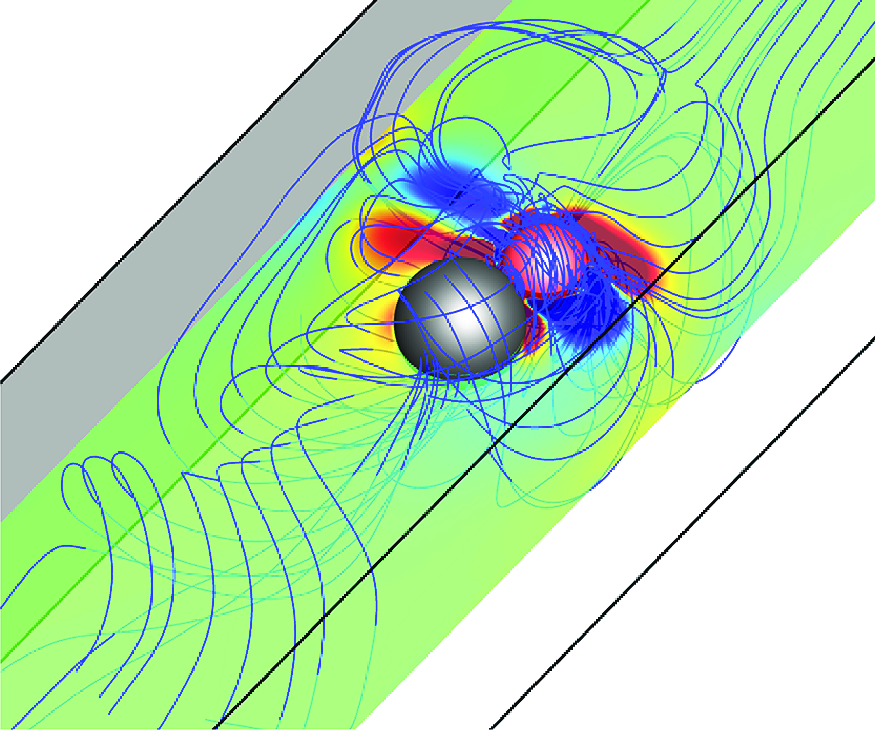
Streamline distributions in the three-dimensional space and vorticity contours in spatial cross-section for (Re p , β, ξ) = (a) (1, 4, 15), single swimmer; (b) (1, –4, 0), AC; (c) (1, –4, 15), AC; (d) (3, –4, 15), AC; (e) (1, –4, 15), single swimmer; (f) (1, –4, 0), CA; (g) (1, –4, 15), CA; (h) (3, –4, 15), CA. The blue arrow represents the swimming direction.

Taking the parameters (Re p , β, ξ) = (3, –4, 15) as an example, figure 10 illustrates the changes of the velocity, spring length and the three-dimensional trajectories of the active swimmer for the AC and CA models when chirality is considered. For the AC model, as depicted in figures 9(d) and 10(a,b), the pusher–cargo (β = –4) undergoes helical oscillations around the channel centre, the trajectory projecting a circular path in the Y–Z plane. The swimming direction of the pusher–cargo is along the negative x-axis, which is defined as the reverse mode. The chiral pusher induces spin and attracts the downstream fluid to generate the spinning streamlines that point towards the cargo, drawing the cargo to the pusher’s head, and the minimum spring length is observed in figures 9(d) and 1 0(a). When the reverse motion occurs, the cargo is attracted by the swimmer, leading to the general conclusion that the reverse mode is considered as a special type of attractive mode.
For Re p = 3, β = –4, ξ = 15, (a,c) the time evolution curves of velocity and spring length for AC and CA models, and (b,d) the three-dimensional oscillation trajectories. The blue arrow represents the swimming direction.

For the CA model, as depicted in figure 10(c,d), the cargo–pusher (β = –4) also undergoes helical oscillations around the channel centre. In this case, the cargo–pusher moves forward along the flow direction with high velocity, opposite to the swimming direction of the pusher–cargo in figure 10(a,b). Here, the chiral pusher in figure 9(h) induces the spinning of the cargo, attracting the upstream fluid to generate the rotating streamlines that point towards the cargo, propelling the cargo towards the pusher’s tail and the attractive mode is also observed.
To analyse the effect of the spin coefficient ξ and β on the cargo-carrying behaviours, figure 11 examines the variation in swimming velocity and spring length for the AC and CA models at Re p = 1.
The correlation between the (a) velocity and (b) spring length variations for the AC and CA models with respect to ξ under the conditions of β = ±1, ±4, ±8.

When the AC model does not keep the reverse motion, the velocity of the pusher–cargo and puller–cargo decreases with increasing ξ, the pusher–cargo velocity is consistently greater than the pullercargo. The velocity difference between them increases (decreases) as |β| increases (ξ increases). At higher values of ξ and β, the puller–cargo starts moving in the reverse direction with the attractive mode earlier than the pusher–cargo, and it also keeps a higher reverse velocity than the pusher–cargo. Interestingly, the velocity of the pusher–cargo approaches the puller–cargo when ξ = 20, indicating that the influence of β is diminished at large spin coefficient, in agreement with the findings of a single swimmer in figure 8(c).
For the CA model, it is interesting to note that the velocity of the cargo–pusher and cargo–puller increases with increasing ξ. Notably, when |β| = 1, the velocities for cargo–pusher and cargo–puller largely overlap. When |β| = 4, 8, the velocity of the cargo–puller is slightly larger than the cargo–pusher, a phenomenon that contrasts to the results of single chiral swimmer and the chiral AC model.
For the AC and CA models, as depicted in figure 11(b), the stabilised spring lengths all decrease with increasing ξ. Beyond a critical value of ξ, the spring length reaches its minimum, transitioning to an attractive mode. In other words, even for the CA model, the upstream cargo will be attracted by the downstream active swimmer, and the attractive mode is observed. The critical ξ for transitioning to the attractive mode depends on β. Overall, pushers exhibit the same critical ξ, while pullers have a slightly lower critical value. This process involves a competition between the self-propulsion of active swimmers and chiral rotation. For the non-chiral puller (pusher), it achieves the self-propelled forward movement through front (rear) driving, which will be different by the effect of chiral rotation. As exemplified by the black arrows and blue dotted arrows between the pusher and cargo in figure 13(g)–13(l), the induced streamlines (black arrows) by the pusher keep the opposite direction to the excited axial vortex (blue dotted arrows) by the chiral rotation. Thus, the effect of axial vortex on the reverse motion is reduced. In contrast, as exemplified by the black arrows in figure 5(g)–5(l), the induced streamlines by the puller keeps the opposite direction as the pusher. As a result, the excited axial vortex between the chiral puller and cargo keep the same direction as the induced streamlines, the puller–cargo has a stronger tendency for reverse motion than the pusher–cargo. This explains why the puller–cargo (cargo–puller) transitions to reverse mode (attraction mode) with the smallest spring distance earlier than the pusher–cargo (cargopusher) in figure 11. Besides, the cargo is always influenced by the negative pressure between the puller and cargo. As the value of β increases, the effect of the negative pressure F p becomes more pronounced, the cargo will be more likely to be attracted by the puller. This results in a smaller critical ξ value for AC (β = 4) compared with AC (β = 1), and the minimum spring length is achieved at ξ = 0 when β = 8.
The correlation between the (a) velocity and (b) spring length variations for the AC and CA models with respect to ξ under the conditions of Re p = 0.1, 1, 3.

Velocity contours and streamline distributions; the vorticity contour and force analysis for AC and CA models when ξ = 15, β = –4 for (a,g) Re p = 0.1, AC; (b,h) Re p = 1, AC; (c,i) Re p = 3, AC; (d,j) Re p = 0.1, CA; (e,k) Re p = 1, CA; (f,l) Re p = 3, CA. The blue arrow represents the swimming direction, the white arrow denotes the spinning, the black arrow and blue dotted arrow represent the induced streamlines by the swimmer and the axial vortices by the spinning swimmer dumbbell, respectively.

To analyse the effect of Re p and ξ on the motion of chiral swimmer dumbbell, figure 12 further compares the changes of swimming velocity and spring length for Re p = 0.1, 1 and 3, |β| = 4. Additionally taking the streamlines and force analyses in figures 9and 13 as examples to explain the mechanism behind the changes of the swimming velocity.
At lower Re p (Re p = 0.1), as depicted in figure 12, the effect of ξ on the variation of swimming velocity and spring length for both the AC and CA models is small. As shown in figure 13(a,d,g,j), the motility of swimmer is weak at (Re p , ξ) = (0.1, 15), resulting in the minimal induced vorticity and hydrodynamic interaction between the swimmer and cargo. They maintain a relatively large distance, the effect of chirality on the cargo-carrying velocity is minimal. As Re p increases to 1 and 3, taking figure 13(b–c,e–f,h–i,k–l) as examples, the influence of ξ on the swimming velocity of the AC and CA models in figure 12(a) is obvious. Therefore, the following analysis will focus on the intrinsic mechanisms behind the changes of velocity when the effects of inertia and chirality are obvious.
For the AC model, the velocity and spring length of pusher–cargo and puller–cargo in the first row of figure 12 is decreased with increasing ξ when Re p = 1 and 3, exhibiting an attractive mode. As shown in figure 9(b), the non-chiral puller–cargo does not generate the spinning streamlines, the velocity gradient induced by the pusher aligns with the carrying cargo when ξ = 0, Re p = 1. Thus the larger vortices in figure 9(b) are observed at the same direction, which will reduce energy consumption and increases the velocity of the pusher–cargo. Interestingly, the swimming velocity for both the pusher–cargo and puller–cargo in figure 12(a) is decreased to a negative value when ξ > 10, and the negative velocity is increased with increasing Re p . This is primarily due to the axial vortices induced by the swimmer’s spin, which will attract the downstream fluid to produce spinning reverse streamlines towards the cargo, thereby creating a reverse thrust and inducing reverse motion. When Re p = 3, the AC model experiences oscillatory motion and fails to stabilise at the channel centre, as illustrated in figure 9(d) and figure 13(c,i). The streamlines induced by the pusher and puller point towards the channel wall, failing to provide effective propulsive force. Additionally, the spinning motion attracts more fluids between the cargo and active swimmer to propel the AC model, i.e. the blue dotted arrows, the faster reverse swimming is observed.
For the CA model, the vortices induced between the upstream cargo and downstream non-chiral pusher have the opposite rotational direction when ξ = 0 and Re p = 1, three recirculation zones on each side of cargo–pusher are formed in figure 9(f), which will increase the energy loss and reduce the swimming velocity. When considering the effect of chirality with Re p = 1, 3 in figure 12(a), the larger the value of ξ, the greater the swimming velocity of the cargo–pusher and cargo–puller, and the reverse motion disappears. The axial vortices produced by the chiral swimmer in figure 9(g,h) will attract the downstream cargo even when the swimmer moves faster than the cargo; the attractive motion mode will be observed in the second row of figure 12(b) when ξ > 10. Due to the spinning motion of the cargo and chiral pusher, as illustrated in figures 9(g) and 13(e,k), the area between the cargo and the pusher’s tail also attracts a large amount of fluids, producing significant axial swirls and providing propulsive force. Moreover, in the CA model, the forces acting on the pusher are all along the flow direction, which will further increase the swimming velocity. As Re p = 3, as shown in figure 9(h) and figure 13(f,l), the effect of spinning motion on the flow field becomes more pronounced than Re p = 1, and the cargopusher exhibits oscillatory motion. The swirls at the tails of the cargo and pusher further increase the swimming velocity.
3.3. Effect of diameter ratio, S
In the aforementioned two sections, both the swimmer and cargo have the same size, which is clearly a special case in practical applications. This chapter further explores the motion modes when the active swimmer carries cargo of different sizes. In this chapter, the active swimmer is fixed at d A = 16 μm, and the cargo is varied as 10 ∼ 64 μm, implying a diameter ratio S = d C /d A = 0.625–4. The influence of the diameter ratio S and the spin coefficient ξ on swimming velocity and spring length are examined when Re p = 1, 3.
For the AC model in the first row of figure 14, the upstream active swimmer approaches the cargo and the spring length is less than the equilibrium length. The spring length is decreased with increasing S when Re p = 1, while the cargo within the present size will always be attracted by the swimmer with the minimum spring length when Re p = 3. When the chirality is not considered, taking (Re p , β, ξ) = (3, –4, 0) as an example, the swimming velocity gradually decreases to zero as the cargo size increases, and the velocity of the pusher–cargo is significantly higher than the non-chiral puller–cargo and other situation when the chirality is considered. Thus, the presence of chirality reduces the swimming velocity of AC model, consistent with the conclusions in § 3.2. When (Re p , ξ) = (1, 5), both the pusher–cargo and puller–cargo with small cargo size maintain forward motion. The swimming velocity is decreased with increasing S, the pusher–cargo still remains greater velocity than the puller–cargo. However, the velocities of the pusher–cargo and puller–cargo approach zero with the attractive mode when S ≥ 3. When ξ = 15, it is interesting to note that the pusher–cargo and puller–cargo with (Re p , S) = (1, 1) or (Re p , S) = (3, 0.625) start the reverse motion. As S is increased to 1.5, the reverse velocity reaches its maximum and the reverse velocity of the puller–cargo is slightly larger than the pusher–cargo, contrary to the conclusion at ξ = 5. When S is further increased, the reverse velocity decreases again due to the increased size of cargo and reaches zero at S = 4. For large S, the model’s terminal velocity approaches 0, invariant to the variations in Re p , β and ξ. This may be because, when the cargo is much larger than the active swimmer, the hydrodynamic resistance of the cargo dominates.
Effect of diameter ratio S on the changes of the (a) swimming velocity and (b) spring length for the AC and CA models under different conditions of Re p , β and ξ.

For the CA model in the second row of figure 14, the larger the diameter ratio S, the smaller the swimming velocity. When S = 4, the cargo-carrying velocity is zero, regardless whether the chirality is considered. When the chirality is not presented, taking (Re p , |β|, ξ) = (3, 4, 0) as an example, the velocities of the cargo–pusher and cargo–puller are significantly lower than the chiral cargo–pusher and cargo–puller with (Re p , |β|, ξ) = (3, 4, 15). This indicates that the chirality increases the swimming velocity, contrary to phenomenon of the AC model. When (Re p , ξ) = (1, 5), the velocities of the cargo–pusher and cargo–puller are similar, as the swimmer moves away from the upstream cargo, and the spring is kept in a stretched state. It is difficult for the swimmer to pull the cargo with large size, leading to the increased spring length. When ξ is increased to 15 with Re p = 1, the velocities of the cargo–pusher and cargo–puller are increased, and the cargo is attracted by the downstream swimmer with the minimum spring length. Interestingly, when (Re p , ξ) = (3, 15), the pusher (puller) carrying the small-sized cargo with S = 0.625 can keep a higher velocity than the single chiral pusher (puller) by 150.2 % (174.2 %). When S < 1.5 (2.0), the cargo is always attracted by the puller’s (pusher’s) spin. As S gradually increases, the upstream cargo is hard to be attracted by the swimmer, the swimmer will move away from the cargo. Consequently, the attractive mode disappears, the final spring distance is increased, the swimming velocity at (Re p , ξ) = (3, 15) is less than the attractive mode when (Re p , ξ) = (1, 15).
To further analyse the impact of ξ and S on the cargo-carrying capacity, figure 15 illustrates the trajectories of the AC and CA models on the cross-section plane at Re p = 3. Note that the cargo’s trajectory exhibits a centre-symmetric relationship with the active swimmer, thus only the trajectories of the pusher are shown in figure 15. The streamlines and vorticity contours of pusher–cargo or cargo–pusher with (Re p , β, ξ) = (3, –4, 15) at different S are compared in figures 16and 17. When considering the chirality, the oscillatory motion mode can be categorised as the gradual ellipsoidal oscillation and the stable circular trajectory, which are exemplified in figure 15(b,f) and figure 15(a,c,d,e), respectively. For both the AC and CA models, the oscillatory mode induced by spin affects the velocity differently. The underlying mechanism will be elucidated in the subsequent sections.
Projections on the Y–Z plane of the swimming trajectories of the AC (first row) and CA (second row) models in the channel. Panels show (Re p , β, ξ, S) = (a) (3, –4, 15, 0.75), AC; (b) (3, –4, 15, 2), AC; (c) (3, –4, 15, 3), AC; (d) (3, –4, 15, 0.75), CA; (e) (3, –4, 15, 2), CA; (f) (3, –4, 0, 0.75), CA.

Streamline distributions in three-dimensional space and vorticity contours of the spatial cross-sections for the swimmer dumbbell with (Re p , β, ξ) = (3, –4, 15), and (a) S = 1.5, AC; (b) S = 4, AC; (c) S = 0.625, CA; (d) S = 4, CA. The blue arrow represents the swimming direction.

When (Re p , β, ξ) = (3, –4, 15), the vorticity contours for the AC and CA models with (a) S = 0.625, AC (b) S = 1.5, AC (c) S = 4, AC (d) S = 0.625, CA (e) S = 1.5, CA (f) S = 4, CA. The blue arrow represents the swimming direction, the white arrow denotes the spinning, the black arrow and blue dotted arrow represent the induced streamlines by the swimmer and the axial vortices by the spinning swimmer dumbbell, respectively.

For the AC model, taking (Re p , β, ξ, S) = (3, –4, 15, 0.75) in figure 15(a) as an example, the pusher–cargo forms a stable circular oscillation trajectory when S = 0.625 ∼ 0.75. Due to the rotational motion of chiral pusher, as depicted in figure 17(a), the surrounding fluid is drawn towards the pusher–cargo by the spin. However, due to the small size of the cargo, the surrounding fluid near the cargo also acts on the pusher (the blue dotted arrow). The combined influence of the spring force, the resistance from the cargo and surrounding fluids, will weaken the self-propulsive force of the pusher–cargo and puller–cargo, and the swimming velocity in figure 14(a) is reduced consequently. When the chirality is absent with (Re p , β, ξ) = (3, –4, 0), there is no axial vortex, the absolute cargo-carrying velocity in figure 14(a) is greater than that at (Re p , β, ξ) = (3, –4, 15) when S ≤ 1.5. With increasing cargo size as S = 1.5 ∼ 2.5, the pusher–cargo in figure 15(b) exhibits a gradual ellipsoidal trajectory. During the spin process of the pusher–cargo, the surrounding fluid attracted by the induced axial vortex from the cargo will act on the pusher, and the larger counter-rotational vortex is observed in figure 16(a). Coupled with the resistance from the spring and cargo, the self-propulsive force of pusher–cargo will be ultimately overcome to move in reverse. When the cargo size is appropriate, such as S = 1.5 in figures 16(a) and 17(b), the axial vortices result in the maximum reverse swimming velocity. When S ≥ 3, the pushercargo in figure 15(c) oscillates with a circular trajectory. Due to the channel confinement, taking S = 4 in figures 16(b) and 17(c) as an example, the streamlines induced by the chiral pusher can only encompass the cargo, affecting the development of the axial vortices, and the surrounding fluid acting on the pusher–cargo is reduced. Moreover, an increase in S leads to a greater overall mass of pusher–cargo, resulting in a decrease in velocity. When S = 4, the pusher–cargo and puller–cargo both keep a zero velocity. Therefore, maintaining the circular (inclined elliptical) trajectory for the AC model will reduce (increase) the swimming velocity.
For the CA model, taking (Re p , β, ξ) = (3, –4, 15) in figure 15(d) as an example, the cargo–pusher oscillates around a stable circular trajectory when S = 0.625 ∼ 0.75. On one hand, all the forces in figure 17(d) acting on the pusher are aligned with the motion direction. On the other hand, as shown in figures 16(c) and 17(d), the cargo’s spin attracts more fluid toward the downstream pusher by the chiral effect. Thus, the swimming velocity is further enhanced, the velocity of chiral cargo–pusher (cargo–puller) at S = 0.625 is approximately 206.2 % (298.7 %) of the single chiral pusher (puller) with (Re p , ξ) = (3, 15), and the oscillatory motion is ultimately observed in figures 15(d) and 16(c). Furthermore, for the non-chiral cargo–pusher with (Re p , β, ξ, S) = (3, –4, 0, 0.75), it keeps the gradual ellipsoidal trajectory in figure 15(f); the velocity of non-chiral cargo–pusher in figure 14(a) is approximately 66.3 % of the chiral cargo–pusher with (Re p , β, ξ, S) = (3, –4, 15, 0.75). Therefore, increasing the chiral effect in the CA model will increase the swimming velocity. As shown in in figures 14(a), 16(d) and 17(f), the cargo–pusher stabilises at the channel centre with nearly zero swimming velocity when S = 4; the active swimmer cannot carry the cargo with large size. Therefore, the swimming velocity of the CA model can be increased by a small amplitude oscillatory trajectory, while it will be reduced by a further increased oscillatory amplitude, consistent with the results of non-chiral CA model in figure 3(f).
Finally, the velocity decay of flow field in front of the CA and AC models are analysed to summarise the hydrodynamic interactions between the swimmer dumbbell and the surrounding fluid, as well as the mechanism on the changes of cargo-carrying velocity. Figure 18(a,b) corresponds to the influence of ξ and S on the far-field fluid velocity of the AC and CA models at Re p = 1, respectively.
Velocity decay of the (a) AC and (b) CA models under different parameters at Re p = 1, the distance r is normalised by the swimmer’s radius a.

For a non-chiral single puller at (β, ξ, S) = (4, 0, 0), as shown by the dotted grey line in figure 18(b), the velocity decays with |u| ≈ O(r −2). Previous related studies (Li, Anca & Ardekani Reference Li, Anca and Ardekani2016; More & Ardekani Reference More and Ardekani2020) also reported that the flow velocity in front of a single squirmer decays as |u| ≈ O(r –2) in an infinite fluid field, as the two terms on the right-hand side of (2.1) represent a stresslet that decays as |u| ≈ O(r –2). On the contrary, a chiral single puller with (β, ξ, S) = (4, 15, 0) in figure 18(a) keeps a slow velocity that decays as |u| ≈ O(r −0.5), and the chirality reduces the swimming velocity. This is consistent well with the conclusion that the more rapid decay of the fluid velocity leads to a larger swimming velocity of squirmers (Ouyang et al. Reference Ouyang, Lin, Yu, Lin and Phan-Thien2022).
For the swimmer dumbbell, the typical velocity decay of the flow field in front of the CA model is much larger than that of AC. For the AC model without chirality, the puller–cargo and pusher–cargo (i.e. the red lines in figure 18 a) exhibit similar velocity decays of |u| ≈ O(r −2.7). Therefore, the velocity in figure 11 depends on the swimmers themselves, the pusher swims faster than the puller. For the CA model without chirality, the velocity decay of the cargo–puller is faster than that of the cargo–pusher (i.e. the red lines in figure 18 b). Consequently, the swimming velocity of cargo–puller in figure 11 is greater than the cargo–pusher.
For the chiral AC model, taking (β, ξ, S) = (±4, 15, 1) in figure 18(a) with blue lines as examples, the velocity of the pusher–cargo decays with |u| ≈ O(r −9.5), and the puller–cargo decays faster than the pusher–cargo. For the chiral CA model under the same flow condition, the cargo–pusher and cargo–puller in figure 18(b) exhibit similar velocity decays of |u| ≈ O(r −10.5). Therefore, the reverse swimming velocity of the puller–cargo in figure 11 is greater than the pusher–cargo, and the cargo-carrying velocity of CA model is greater than the AC model.
When considering the effect of S, it is interesting to note that the absolute velocity of the AC model with (β, ξ, S) = (±4, 15, 1.5) is significantly larger than the AC model with (β, ξ, S) = (±4, 15, 1), cf. the green lines and blue lines in figure 18(a), respectively. The AC model exhibits a slower velocity decay than the CA model, leading to the higher absolute velocity of the CA model than the AC model. The effect of the pusher and puller on the changes in velocity decay becomes less pronounced under the consideration of chirality. Consequently, the velocity difference between the pusher and puller in the AC and CA models in figure 14 does not exhibit significant changes at large chiral effect.
3.4. Phase diagram of the motion behaviour
The above studies indicate that the performance of the AC and CA models for both puller and pusher with large chirality have similar velocities. Therefore, this chapter only summarises the effects of Re p , ξ and S on the motion mode of the pusher–cargo and cargo–pusher (β = –4) when Re p = 1 ∼ 3, ξ = 0 ∼ 20 and S = 0.75 ∼ 4; a phase diagram of the motion mode is presented in figure 19. Due to the overlap between some modes, certain points in the phase diagram are marked with dual symbols. The existing motion modes are summarised into four categories:
-
(i) Steady-state mode: the swimmer dumbbell is able to swim steadily near the channel centre with small transverse oscillations (less than 0.1d A ), and the spring keeps the stretch/compression state. The steady-state mode in figure 19 appears within the range of lower value of ξ (ξ ≤ 10), especially at ξ = 0. The CA model is more prone to keep the steady-state mode than the AC model; and they are more likely to maintain a steady-state mode at Re p = 1 than at Re p = 3.
-
(ii) Attraction mode: due to the self-propulsive force from the pusher or the attraction induced by the axial vortices near the spinning AC and CA models, the cargo is always attracted by the chiral pusher with the minimum spring length. As shown in figure 19, the attraction mode is prevalent in the swimmer dumbbell with spin motion, particularly for the CA model with S = 2 ∼ 4.
-
(iii) Oscillation mode: due to the interaction between the swimmer and cargo, the swimmer dumbbell exhibits significant oscillation trajectories in the Y–Z plane (greater than 0.1d A ), as depicted in figures 3(e,f), 10(b,d) and 15. As shown in figure 19, the oscillation mode predominantly occurs when S = 0.75 ∼ 2, and it is not observed when S = 4. Moreover, the oscillation mode becomes more prevalent as ξ increases (ξ > 10), particularly at high Re p .
-
(iv) Reverse mode: the swimmer dumbbell achieves reverse motion due to the axial vortices induced by the spinning motion of pusher–cargo and puller–cargo, the spring length also reaches its minimum. It can also be considered as a special type of attraction mode. As shown in figure 19, the CA model never keeps the reverse motion, only the AC model keeps the reverse motion when ξ ≥ 10. However, the reverse mode disappears again when diameter ratio is enhanced as S = 4.
Phase diagram of the motion modes for the pusher–cargo and cargo–pusher.

4. Summary
Cargo carrying by a spring connected chiral micro-swimmer in a square channel is numerical studied by the three-dimensional LBM and a chiral squirmer model. Depending on the relative positions of the active swimmer and cargo, the model is categorised into the AC and CA models. The study investigates the effects of the driving type (β), swimming Reynolds number (Re p ), spin coefficient (ξ) and diameter ratio (S) on the changes of the cargo-carrying velocity, spring length and motion modes. Four kinds of interesting motion modes are observed in this work. The conclusions are summarised as follows:
-
(i) For the non-chiral swimmer dumbbell, the velocity of the AC (CA) model is decreased (increased) gradually with increasing β at a small Re p , and the optimal combinations for maximising swimming velocity are the pusher–cargo and cargo–puller configurations when Re p = 0.1 ∼ 1. When Re p is enhanced, and the velocities of both the AC and CA models are decreased with increasing β, the swimming velocities of the pusher–cargo, puller–cargo and cargo–pusher is increased, while the velocity of the cargo–puller is gradually decreased.
-
(ii) For the chiral swimmer, the velocity of the AC model and single swimmer is decreased as the chirality is enhanced, while the velocity of the CA model keeps an interesting increment. The impact of ξ on swimming velocity becomes more pronounced as Re p increases. Moreover, when ξ exceeds a certain value, due to the axial vortices generated by spinning, the CA model changes from the steady-state to attractive mode, the reverse motion mode for AC model is firstly found in our work.
-
(iii) The impact of the diameter ratio S on the AC and CA models is complex, a variety of oscillatory trajectories will appear under different ξ and S. When ξ is small, the large S leads to a decrease in the swimming velocity of the AC model. When S = 0.625 ∼ 1.5 and ξ is large, the larger S results in a greater reverse swimming velocity of the AC model, while a smaller reverse velocity and even zero velocity will be observed as S > 1.5. For the CA model, the larger S leads to a smaller velocity and the reverse motion is not observed.
Overall, this study discusses strategies for enhancing the cargo-carrying capacity of swimmer dumbbells and provides a reference for optimising corresponding parameters. The results contribute to a comprehensive understanding on the locomotion strategies and associated hydrodynamic mechanisms of micro-swimmer in confined space.
The impact of spring coefficient on the motion behaviours for pusher–cargo with (Re p , β, ξ, S) = (3, –4, 15, 1). (a) The relationship between the swimming velocity, spring length and the spring coefficient; (b–g) The trajectory projection in the Y–Z plane under different spring coefficients.

Funding
This work was supported by the Major Program of the National Natural Science Foundation of China with Grant No. 12132015, National Natural Science Foundation of China with Grant No. 12202392, National Natural Science Foundation of China with Grant No. 52476039, National Natural Science Foundation of China with Grant No. 12372251, National Natural Science Foundation of China with Grant No. 12302340, Science Foundation of Zhejiang Sci-Tech University (ZSTU) under Grant No. 25242160-Y.
Declaration of interests
The authors report no conflict of interest.
Appendix A. The effect of spring coefficient, k
To investigate the effects of the spring coefficient on the model’s overall swimming velocity, spring length and the trajectory projection in the Y–Z plane, we added relevant numerical analysis, taking the pusher–cargo model with (Re p , β, ξ, S) = (3, –4, 15, 1) as an example. The results in the figure 20 indicate that varying the spring coefficient over a wide range does not have a decisive impact on the reverse motion. When the spring coefficient is small (k < 1), it has no effect on swimming velocity and final spring length; the typical spring coefficient (k = 0.01) is chosen in this article. However, at higher elastic coefficients (k ≥ 1), the reverse swimming velocity slightly decreases, the swimming velocity of pusher–cargo is consistent with the pusher–cargo that is connected by the rigid rod, which is also in line with expectations. The trajectory projection in the Y–Z plane in figure 20(b–e) shows that the spring coefficient does not fundamentally affect the model’s overall helical oscillating swimming mode, the oscillation amplitude in the Y–Z plane is enhanced when the spring elastic coefficients is increased with the rigid rod.



