1. Introduction
In his famous pipe flow experiment, Reynolds (Reference Reynolds1883) observed transition to turbulence and showed that the critical value of a governing non-dimensional parameter, to be later termed the Reynolds number, was strongly dependent on the level of external noise. However, linear stability theory predicts the Hagen–Poiseuille flow to be asymptotically stable for any value of
 $\mathit{Re}$
(Schmid & Henningson Reference Schmid and Henningson2001). It is now well understood that linear stability theory successfully captures bifurcations and instability mechanisms for some flows (e.g. Rayleigh–Bénard convection, Taylor–Couette flow between rotating cylinders, or flow past a cylinder), but fails for other flows: the Navier–Stokes equations which govern fluid motion constitute a non-normal system, able to amplify perturbations through non-modal mechanisms (Trefethen et al.
Reference Trefethen, Trefethen, Reddy and Driscoll1993); then, if amplification is large enough it may drive the system away from linearly stable solutions. Non-normal stable systems can exhibit large transient growth
 $G(t)=\Vert \boldsymbol{u}(\boldsymbol{x},t)\Vert /\Vert \boldsymbol{u}(\boldsymbol{x},0)\Vert$
, i.e. temporary amplification of initial conditions
 $\boldsymbol{u}(\boldsymbol{x},0)$
, as well as large harmonic gain
 $G({\it\omega})=\Vert \boldsymbol{u}(\boldsymbol{x})\Vert /\Vert \boldsymbol{f}(\boldsymbol{x})\Vert$
, i.e. asymptotic amplification of the response
 $\boldsymbol{u}(\boldsymbol{x})\cos ({\it\omega}t)$
to external harmonic forcing
 $\boldsymbol{f}(\boldsymbol{x})\cos ({\it\omega}t)$
. Classical linear algebra techniques allow one to find the largest amplification possible, together with optimal perturbations, i.e. those specific structures associated with maximal transient growth or harmonic gain. Extensive literature exists about the calculation of transient growth (Butler & Farrell Reference Butler and Farrell1992; Corbett & Bottaro Reference Corbett and Bottaro2000; Blackburn, Barkley & Sherwin Reference Blackburn, Barkley and Sherwin2008) and harmonic gain (Åkervik et al.
Reference Åkervik, Ehrenstein, Gallaire and Henningson2008; Alizard, Cherubini & Robinet Reference Alizard, Cherubini and Robinet2009; Dergham, Sipp & Robinet Reference Dergham, Sipp and Robinet2013; Garnaud et al.
Reference Garnaud, Lesshafft, Schmid and Huerre2013; Sipp & Marquet Reference Sipp and Marquet2013).
A question of fundamental importance is whether these non-modal amplification mechanisms are sensitive: if they are significantly altered by small flow modifications, one can design control strategies with a wide variety of applications, such as enhancing mixing, improving aerodynamic performance, and reducing noise and vibration. To investigate this point, adjoint methods are particularly well suited, as they provide maps of sensitivity showing regions where a given quantity of interest is the most affected by small-amplitude flow modification or steady control. Since the actual modified flow need not be computed, sensitivity analysis allows a fast and systematic control design, without resorting to time-consuming parameter studies. In the context of linearly unstable flows, Hill (Reference Hill1992) used such a variational technique to derive the gradient of the leading eigenvalue with respect to flow modification and to steady control, and successfully reproduced maps of vortex shedding suppression obtained experimentally by Strykowski & Sreenivasan (Reference Strykowski and Sreenivasan1990). Similar methods were later applied to eigenvalues in several parallel and non-parallel configurations (Bottaro, Corbett & Luchini Reference Bottaro, Corbett and Luchini2003; Marquet, Sipp & Jacquin Reference Marquet, Sipp and Jacquin2008; Meliga, Sipp & Chomaz Reference Meliga, Sipp and Chomaz2010). For unstable flows, Brandt et al. (Reference Brandt, Sipp, Pralits and Marquet2011) followed a similar technique to derive an expression for the sensitivity of the optimal harmonic gain
 $G({\it\omega})$
with respect to flow modification and to steady control. They applied their formula to parallel and non-parallel flat-plate boundary layers and discussed the sensitivity of
 $G({\it\omega})$
for Tollmien–Schlichting and lift-up instability mechanisms. Boujo, Ehrenstein & Gallaire (Reference Boujo, Ehrenstein and Gallaire2013) used this method to identify sensitive regions in the separated flow past a wall-mounted bump, and designed a simple open-loop wall control able to delay noise-induced subcritical transition. They observed, however, that sensitivity to volume control was dependent on frequency, indicating that a given control could reduce
 $G({\it\omega})$
at some frequencies but increase it at others. In this case, the effect of control on the overall response of the stochastically driven flow is unclear, and control design is not easy.
In the present study, we extend sensitivity methods for linearly stable flows in two ways. First, we compute the sensitivity of amplification when the flow is subject to stochastic forcing rather than harmonic forcing. This step takes advantage of the relation between stochastic and harmonic amplification (Farrell & Ioannou Reference Farrell and Ioannou1996). It allows us to consider the overall response of the flow to external noise, and to combine sensitivities at individual frequencies into a single sensitivity. Second, we derive an expression for the sensitivity of amplification when the flow is forced at the inlet rather than in the whole domain, with the aim of dealing with a realistic model of incoming perturbations in convectively unstable open flows. The method is illustrated with the two-dimensional incompressible flow past a backward-facing step, a canonical noise amplifier flow.
This flow has been studied extensively experimentally and numerically for a wide variety of Reynolds numbers and expansion ratios. For instance, Armaly et al. (Reference Armaly, Durst, Pereira and Schönung1983) used laser-Doppler velocimetry (LDV) to measure the position of stagnation points in laminar and turbulent regimes, and discussed the appearance of three-dimensionality. Beaudoin et al. (Reference Beaudoin, Cadot, Aider and Wesfreid2004) investigated in more detail three-dimensional effects with particle image velocimetry (PIV). Kaiktsis, Karniadakis & Orszag (Reference Kaiktsis, Karniadakis and Orszag1996) performed two-dimensional direct numerical simulations as well as local and global linear stability analyses, and studied the response to impulsive and harmonic forcing in the volume or at the inlet.
Barkley, Gomes & Henderson (Reference Barkley, Gomes and Henderson2002) performed a three-dimensional linear stability analysis for a step-to-outlet expansion ratio
 ${\it\Gamma}=0.5$
and showed the three-dimensional character of the first globally unstable mode at
 $\mathit{Re}_{c}=748$
, the flow remaining globally stable to two-dimensional perturbations due to the convective nature of the shear layer instability. Lanzerstorfer & Kuhlmann (Reference Lanzerstorfer and Kuhlmann2012) found
 $\mathit{Re}_{c}=714$
for
 ${\it\Gamma}=0.5$
, and extended the stability analysis to smaller and larger expansion ratios. Blackburn et al. (Reference Blackburn, Barkley and Sherwin2008) studied convective instabilities for
 ${\it\Gamma}=0.5$
. Computing optimal transient growth, they observed three-dimensional values slightly larger than the two-dimensional one, for large wavelengths and with very similar flow structures. Furthermore, white-noise inlet velocity fluctuations in a direct numerical simulation below the global instability threshold (
 $\mathit{Re}=500$
) resulted in ‘predominantly two-dimensional wave packets whose properties are related to the optimal disturbances’ found in the transient growth analysis. Finally, Marquet & Sipp (Reference Marquet, Sipp, Schlatter and Henningson2010) investigated the optimal harmonic response for
 ${\it\Gamma}=0.5$
,
 $\mathit{Re}=500$
, in the two-dimensional flow, and found values of the most amplified frequency and the streamwise location of maximum response consistent with results from the transient growth analysis and the perturbed direct numerical simulation of Blackburn et al. (Reference Blackburn, Barkley and Sherwin2008).
This paper is organised as follows. Section 2 recalls how to characterise the response to harmonic and stochastic forcing in the volume and at the inlet, and presents how to compute the sensitivity of harmonic and stochastic gains. Section 3 details the numerical method and its validation. The harmonic response in the backward-facing step flow for
 ${\it\Gamma}=0.5$
and several values of
 $\mathit{Re}$
is presented in § 4, where a connection with local stability analysis is also established. Results from the sensitivity analysis of harmonic and stochastic responses are given in § 5 for
 ${\it\Gamma}=0.5$
,
 $\mathit{Re}=500$
. Maps of sensitivity to volume control and wall control are presented in §§ 5.1 and 5.2, respectively. The analysis shows the dominant role of the optimal harmonic response at the optimal frequency. Validation against nonlinear calculations is also presented (§ 5.2.2), as well as an application to passive wall control (§ 5.2.3). Finally, § 6 discusses the link between the sensitivities of noise amplification and recirculation length, and investigates other
 ${\it\Gamma}{-}\mathit{Re}$
configurations. Conclusions are drawn in § 7.
2. Problem formulation
2.1. Flow configuration
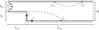
We consider the two-dimensional flow over a backward-facing step, shown schematically in figure 1. Geometrical parameters are the inlet height
 $h_{in}$
, the step height
 $h_{s}$
, and the outlet height
 $H=h_{s}+h_{in}$
, which can be combined into a single governing parameter: the step-to-outlet expansion ratio
 ${\it\Gamma}=h_{s}/H$
or, equivalently, the outlet-to-inlet expansion ratio
 $e=H/h_{in}=1/(1-{\it\Gamma})$
. Throughout this paper we will consider the classical geometry
 ${\it\Gamma}=0.5$
(
 $e=2$
), and a smaller step characterised by
 ${\it\Gamma}=0.3$
(
 $e\simeq 1.43$
). The vertical wall and outlet lower wall define the
 $x=0$
and
 $y=0$
axes respectively. The incoming flow is assumed to have a fully developed parabolic Poiseuille profile of maximum (centreline) velocity
 $U_{\infty }$
at the inlet
 ${\it\Gamma}_{in}$
located at
 $x=-L_{in}$
, while the outlet is at
 $x=L_{out}$
. The reference length is chosen as
 $L=H/2$
and the reference velocity as
 $U_{\infty }$
. The Reynolds number is consequently defined as
 $\mathit{Re}=LU_{\infty }/{\it\nu}$
, where
 ${\it\nu}$
is the fluid kinematic viscosity.
Sketch of the geometry, including the separation and reattachment points.

The steady-state base flow
 $(\boldsymbol{U}_{b},P_{b})$
is solution of the stationary incompressible Navier–Stokes equations in the domain
 ${\it\Omega}$
, with no-slip boundary conditions at the walls
 ${\it\Gamma}_{w}$
:
 $$\begin{eqnarray}\left.\begin{array}{@{}c@{}}\boldsymbol{{\rm\nabla}}\boldsymbol{\cdot }\boldsymbol{U}_{b}=0,\\ \boldsymbol{U}_{b}\boldsymbol{\cdot }\boldsymbol{{\rm\nabla}}\boldsymbol{U}_{b}+\boldsymbol{{\rm\nabla}}P_{b}-\mathit{Re}^{-1}{\rm\nabla}^{2}\boldsymbol{U}_{b}=0,\\ \boldsymbol{U}_{b}=0\quad \text{on }{\it\Gamma}_{w}.\end{array}\right\}\end{eqnarray}$$
2.2. Response to forcing
In the following, we consider the response of a stable steady-state base flow to forcing. The focus of this paper is on stochastic inlet forcing, but we mention harmonic and/or volume forcing to help understanding and highlight differences. More details can be found for example in Farrell & Ioannou (Reference Farrell and Ioannou1996) and Schmid & Henningson (Reference Schmid and Henningson2001). We first recall how the response to a small-amplitude harmonic forcing
 $\boldsymbol{f}^{\prime }(\boldsymbol{x},t)=\boldsymbol{f}(\boldsymbol{x})\text{e}^{\text{i}{\it\omega}t}$
is characterised. If the flow is linearly stable, the asymptotic response is also harmonic at the same frequency. The forcing therefore introduces perturbations
 $(\boldsymbol{u}^{\prime },p^{\prime })(\boldsymbol{x},t)=(\boldsymbol{u},p)(\boldsymbol{x})\text{e}^{\text{i}{\it\omega}t}$
to the base flow whose dynamics is governed by the linearised equations
 $$\begin{eqnarray}\left.\begin{array}{@{}c@{}}\boldsymbol{{\rm\nabla}}\boldsymbol{\cdot }\boldsymbol{u}_{vol}=0,\\ \text{i}{\it\omega}\boldsymbol{u}_{vol}+\boldsymbol{U}_{b}\boldsymbol{\cdot }\boldsymbol{{\rm\nabla}}\boldsymbol{u}_{vol}+\boldsymbol{u}_{vol}\boldsymbol{\cdot }\boldsymbol{{\rm\nabla}}\boldsymbol{U}_{b}+\boldsymbol{{\rm\nabla}}p_{vol}-\mathit{Re}^{-1}{\rm\nabla}^{2}\boldsymbol{u}_{vol}=\boldsymbol{f}_{vol},\\ \boldsymbol{u}_{vol}=0\quad \text{on }{\it\Gamma}_{in}\cup {\it\Gamma}_{w}\end{array}\right\}\end{eqnarray}$$
for volume forcing in
 ${\it\Omega}$
, and by
 $$\begin{eqnarray}\left.\begin{array}{@{}c@{}}\boldsymbol{{\rm\nabla}}\boldsymbol{\cdot }\boldsymbol{u}_{in}=0,\\ \text{i}{\it\omega}\boldsymbol{u}_{in}+\boldsymbol{U}_{b}\boldsymbol{\cdot }\boldsymbol{{\rm\nabla}}\boldsymbol{u}_{in}+\boldsymbol{u}_{in}\boldsymbol{\cdot }\boldsymbol{{\rm\nabla}}\boldsymbol{U}_{b}+\boldsymbol{{\rm\nabla}}p_{in}-\mathit{Re}^{-1}{\rm\nabla}^{2}\boldsymbol{u}_{in}=0,\\ \boldsymbol{u}_{in}=\boldsymbol{f}_{in}\quad \text{on }{\it\Gamma}_{in},\\ \boldsymbol{u}_{in}=0\quad \text{on }{\it\Gamma}_{w}\end{array}\right\}\end{eqnarray}$$
for inlet forcing on
 ${\it\Gamma}_{in}$
(Garnaud et al.
Reference Garnaud, Lesshafft, Schmid and Huerre2013). We formally write (2.2) as
 $\boldsymbol{u}_{vol}=\mathscr{R}_{vol}({\it\omega})\boldsymbol{f}_{vol}$
and (2.3) as
 $\boldsymbol{u}_{in}=\mathscr{R}_{in}({\it\omega})\boldsymbol{f}_{in}$
, where in both cases
 $\mathscr{R}({\it\omega})$
is the resolvent operator. For a given forcing, one simply needs to invert a linear system to obtain the response. We introduce the usual Hermitian scalar product
 $(\boldsymbol{a}\mid \boldsymbol{b})=\int _{{\it\Omega}}\overline{\boldsymbol{a}}\boldsymbol{\cdot }\boldsymbol{b}\text{d}{\it\Omega}=\int _{{\it\Omega}}\boldsymbol{a}^{H}\boldsymbol{b}\text{d}{\it\Omega}$
or
 $(\boldsymbol{a}\mid \boldsymbol{b})=\int _{\partial {\it\Omega}}\overline{\boldsymbol{a}}\boldsymbol{\cdot }\boldsymbol{b}\text{d}{\it\Gamma}=\int _{\partial {\it\Omega}}\boldsymbol{a}^{H}\boldsymbol{b}\text{d}{\it\Gamma}$
for complex fields defined respectively in the domain or on (part or all of) the boundary, where
 $\overline{\boldsymbol{\cdot }}$
and
 $\boldsymbol{\cdot }^{H}$
stand for conjugate and conjugate transpose. The norm induced by this scalar product is used to measure amplification in the flow, or harmonic gain
 $G({\it\omega})=\Vert \boldsymbol{u}\Vert /\Vert \,\boldsymbol{f}\Vert$
. A natural quantity to look at is the largest value the gain may take, or optimal gain, together with the associated ‘most dangerous’ forcing, or optimal forcing. This worst-case scenario is classically investigated by introducing the adjoint operator of the resolvent, and recasting the harmonic gain as a Rayleigh quotient:
 $$\begin{eqnarray}G^{2}({\it\omega})=\frac{\Vert \boldsymbol{u}\Vert ^{2}}{\Vert \,\boldsymbol{f}\Vert ^{2}}=\frac{(\mathscr{R}\boldsymbol{f}\mid \mathscr{R}\boldsymbol{f})}{(\,\boldsymbol{f}\mid \boldsymbol{f})}=\frac{(\mathscr{R}^{\dagger }\mathscr{R}\boldsymbol{f}\mid \,\boldsymbol{f})}{(\,\boldsymbol{f}\mid \boldsymbol{f})}.\end{eqnarray}$$
The largest value of
 $G$
is by definition the induced norm of the resolvent
 $\Vert \mathscr{R}\Vert$
, which can be calculated as the largest singular value of
 $\mathscr{R}$
. Alternatively, solving the symmetric eigenvalue problem
 $\mathscr{R}^{\dagger }\mathscr{R}\boldsymbol{f}_{k}=G_{k}^{2}\,\boldsymbol{f}_{k}$
yields a set of real positive eigenvalues
 $G_{1}^{2}\geqslant G_{2}^{2}\geqslant G_{3}^{2}\cdots \,$
and a set of orthogonal eigenvectors
 $\boldsymbol{f}_{k}$
, from which one deduces the optimal gain:
 $$\begin{eqnarray}G_{1}({\it\omega})=\max _{\boldsymbol{f}}\frac{\Vert \boldsymbol{u}\Vert }{\Vert \,\boldsymbol{f}\Vert }=\frac{\Vert \boldsymbol{u}_{1}\Vert }{\Vert \,\boldsymbol{f}_{1}\Vert }.\end{eqnarray}$$
The response of the flow to the optimal forcing is the optimal response
 $\boldsymbol{u}_{1}=\mathscr{R}\boldsymbol{f}_{1}$
. One can similarly define sub-optimal gains, forcings and responses as
 $G_{k}=\Vert \boldsymbol{u}_{k}\Vert /\Vert \,\boldsymbol{f}_{k}\Vert$
,
 $\boldsymbol{u}_{k}=\mathscr{R}\boldsymbol{f}_{k}$
(Dergham et al.
Reference Dergham, Sipp and Robinet2013; Garnaud et al.
Reference Garnaud, Lesshafft, Schmid and Huerre2013).
We now turn our attention to stochastic forcing. We assume that the flow is continuously forced by componentwise-uncorrelated white noise of unit variance,
 $\boldsymbol{f}^{\prime }(\boldsymbol{x},t)=\int _{-\infty }^{\infty }\boldsymbol{f}(\boldsymbol{x},{\it\omega})\text{e}^{\text{i}{\it\omega}t}\text{d}{\it\omega}$
, such that
 $\mathscr{E}(\,f_{j}(\boldsymbol{x},{\it\omega}_{1})f_{k}(\boldsymbol{x},{\it\omega}_{2}))={\it\delta}_{jk}{\it\delta}({\it\omega}_{1}-{\it\omega}_{2})/2{\rm\pi}$
where
 $\mathscr{E}(\cdot )$
denotes the mean or expected value of a random variable. Unless one has specific knowledge about temporal and spatial characteristics of incoming perturbations, this assumption has the advantage of being both reasonable and simple. The stochastic response is then characterised by the stationary ensemble variance (Farrell & Ioannou Reference Farrell and Ioannou1996; Zhou, Doyle & Glover Reference Zhou, Doyle and Glover1996)
 $$\begin{eqnarray}E=\mathscr{E}\left(\Vert \boldsymbol{u}\Vert _{2}^{2}\right)=\frac{1}{2{\rm\pi}}\int _{-\infty }^{\infty }\text{Tr}(\mathscr{R}({\it\omega})^{\dagger }\mathscr{R}({\it\omega}))\text{d}{\it\omega},\end{eqnarray}$$
which can be expressed in terms of eigenvalues of
 $\mathscr{R}^{\dagger }\mathscr{R}$
:
 $$\begin{eqnarray}E=\frac{1}{2{\rm\pi}}\int _{-\infty }^{\infty }\mathop{\sum }_{k}G_{k}^{2}({\it\omega})\text{d}{\it\omega}=\frac{1}{{\rm\pi}}\int _{0}^{\infty }\mathop{\sum }_{k}G_{k}^{2}({\it\omega})\text{d}{\it\omega}=\mathop{\sum }_{k}I_{k}.\end{eqnarray}$$
For convenience we call
 $E$
the stochastic gain, in contrast to the harmonic gain
 $G({\it\omega})$
.
2.3. Sensitivity of harmonic and stochastic gain
Since non-normal flows have the potential for large amplification of perturbations, one way to delay transition to unsteadiness and turbulence is to apply a control, for instance steady control in the volume or at the wall, with the aim of reducing harmonic and stochastic gains. In this section we give the expressions for sensitivities of harmonic/stochastic gains with respect to steady flow modification and steady control. These sensitivities are gradients which predict the effect of small-amplitude flow modification and control on the asymptotic amplification of harmonic/stochastic perturbations, and allow one to identify regions of the domain
 ${\it\Omega}$
and of the wall
 ${\it\Gamma}_{w}$
where gains are the most sensitive, i.e. can be modified most easily. It is worth stressing that the time-dependent forcing
 $\boldsymbol{f}$
is an external unwanted perturbation undergoing amplification as described in § 2.2, while the steady control
 $\boldsymbol{C}$
or
 $\boldsymbol{U}_{c}$
introduced in this section is applied intentionally in the flow or at the wall with the aim of reducing amplification.
Starting with harmonic gain, we look for the two-dimensional sensitivity field
 $\boldsymbol{{\rm\nabla}}_{\boldsymbol{U}}G_{1}^{2}$
defined in
 ${\it\Omega}$
such that a modification
 ${\bf\delta}\boldsymbol{U}$
of the base flow induces a variation of the (squared) optimal gain
 $$\begin{eqnarray}{\it\delta}G_{1}^{2}=(\boldsymbol{{\rm\nabla}}_{\boldsymbol{U}}G_{1}^{2}\mid {\bf\delta}\boldsymbol{U}).\end{eqnarray}$$
Using a Lagrangian-based variational technique, Brandt et al. (Reference Brandt, Sipp, Pralits and Marquet2011) derived an expression for the sensitivity of the optimal harmonic gain for the case of volume forcing. This expression is straightforwardly generalised to any sub-optimal gain
 $G_{vol,k},\ k>1$
, replacing the optimal forcing
 $\boldsymbol{f}_{vol,1}$
and optimal response
 $\boldsymbol{u}_{vol,1}$
by the
 $k$
th sub-optimal forcing and response:
 $$\begin{eqnarray}\boldsymbol{{\rm\nabla}}_{\boldsymbol{U}}G_{vol,k}^{2}=2G_{vol,k}^{2}\,\text{Re}\{-\boldsymbol{{\rm\nabla}}\boldsymbol{u}_{vol,k}^{H}\,\boldsymbol{f}_{vol,k}+\boldsymbol{{\rm\nabla}}\boldsymbol{f}_{vol,k}\,\overline{\boldsymbol{u}}_{vol,k}\}.\end{eqnarray}$$
Using the same technique, we derived an expression for the case of inlet forcing:
 $$\begin{eqnarray}\boldsymbol{{\rm\nabla}}_{\boldsymbol{U}}G_{in,k}^{2}=2\,\text{Re}\{-\boldsymbol{{\rm\nabla}}\boldsymbol{u}_{in,k}^{H}\,\boldsymbol{u}_{in,k}^{\dagger }+\boldsymbol{{\rm\nabla}}\boldsymbol{u}_{in,k}^{\dagger }\,\overline{\boldsymbol{u}}_{in,k}\}\end{eqnarray}$$
where the adjoint perturbation
 $(\boldsymbol{u}_{in,k}^{\dagger },p_{in,k}^{\dagger })$
is a solution of the linear system
 $\boldsymbol{u}_{in,k}^{\dagger }=\mathscr{R}_{vol}^{\dagger }\boldsymbol{u}_{in,k}$
:
 $$\begin{eqnarray}\left.\begin{array}{@{}c@{}}\boldsymbol{{\rm\nabla}}\boldsymbol{\cdot }\boldsymbol{u}_{in,k}^{\dagger }=0,\\ -\text{i}{\it\omega}\boldsymbol{u}_{in,k}^{\dagger }+\boldsymbol{U}_{b}\boldsymbol{\cdot }\boldsymbol{{\rm\nabla}}\boldsymbol{u}_{in,k}^{\dagger }-\boldsymbol{u}_{in,k}^{\dagger }\boldsymbol{\cdot }\boldsymbol{{\rm\nabla}}\boldsymbol{U}_{b}^{T}+\boldsymbol{{\rm\nabla}}p_{in,k}^{\dagger }+\mathit{Re}^{-1}{\rm\nabla}^{2}\boldsymbol{u}_{in,k}^{\dagger }=\boldsymbol{u}_{in,k},\\ \boldsymbol{u}_{in,k}^{\dagger }=0\quad \text{on }{\it\Gamma}_{in}\cup {\it\Gamma}_{w}.\end{array}\right\}\end{eqnarray}$$
In the case of sensitivity to volume forcing (2.9), no adjoint variable needs to be computed (Brandt et al.
Reference Brandt, Sipp, Pralits and Marquet2011). This comes from the fact that the operator
 $\mathscr{R}_{vol}^{\dagger }\mathscr{R}_{vol}$
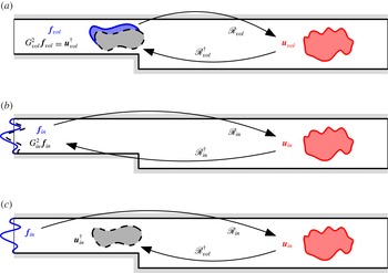
involved in the volume forcing problem and associated gain sensitivity is self-adjoint (see figure 2
a). In other words, even though an adjoint perturbation has to be included in the Lagrangian a priori, calculations show that it can be replaced by
 $G_{vol}^{2}\,\boldsymbol{f}_{vol}$
: indeed, (2.2) is
 $\boldsymbol{u}_{vol}=\mathscr{R}_{vol}\,\boldsymbol{f}_{vol}$
and implies
 $\mathscr{R}_{vol}^{\dagger }\,\boldsymbol{u}_{vol}=\mathscr{R}_{vol}^{\dagger }\mathscr{R}_{vol}\,\boldsymbol{f}_{vol}=G_{vol}^{2}\,\boldsymbol{f}_{vol}$
; at the same time, detailed calculations lead to the adjoint perturbation equation
 $\boldsymbol{u}_{vol}^{\dagger }=\mathscr{R}_{vol}^{\dagger }\boldsymbol{u}_{vol}$
, and therefore
 $\boldsymbol{u}_{vol}^{\dagger }=G_{vol,k}^{2}\,\boldsymbol{f}_{vol}$
. The situation is quite different for inlet forcing. The operator
 $\mathscr{R}_{in}^{\dagger }\mathscr{R}_{in}$
involved in the inlet forcing problem is self-adjoint too (figure 2
b), but the operator
 $\mathscr{R}_{vol}^{\dagger }\mathscr{R}_{in}$
needed to obtain the associated sensitivity is not (figure 2
c). Consequently, the adjoint perturbation
 $(\boldsymbol{u}_{in}^{\dagger },p_{in}^{\dagger })$
which appears in the expression for sensitivity to inlet forcing (2.10) has to be computed on its own. Interestingly, note that although we are dealing with inlet forcing, the adjoint perturbation is a solution of an equation forced in the volume by the response
 $\boldsymbol{u}_{in}$
.
Quantities and operators involved in the computation of the harmonic gain and of its sensitivity. (a) In the case of volume forcing, the gain is given by
 $G_{vol}^{2}\,\boldsymbol{f}_{vol}=\mathscr{R}_{vol}^{\dagger }\mathscr{R}_{vol}\,\boldsymbol{f}_{vol}=\mathscr{R}_{vol}^{\dagger }\boldsymbol{u}_{vol}$
, the operator
 $\mathscr{R}_{vol}^{\dagger }\mathscr{R}_{vol}$
is self-adjoint, and the adjoint perturbation
 $\boldsymbol{u}_{vol}^{\dagger }=G_{vol}^{2}\,\boldsymbol{f}_{vol}$
does not need to be computed to evaluate the gain sensitivity (2.9). (b) In the case of inlet forcing, the gain is given by
 $G_{in}^{2}\,\boldsymbol{f}_{in}=\mathscr{R}_{in}^{\dagger }\mathscr{R}_{in}\,\boldsymbol{f}_{in}=\mathscr{R}_{in}^{\dagger }\boldsymbol{u}_{in}$
, where the operator
 $\mathscr{R}_{in}^{\dagger }\mathscr{R}_{in}$
is self-adjoint; (c) however, in order to evaluate the gain sensitivity (2.10) the adjoint perturbation
 $\boldsymbol{u}_{in}^{\dagger }=\mathscr{R}_{vol}^{\dagger }\boldsymbol{u}_{in}$
must be computed explicitly because the operator
 $\mathscr{R}_{vol}^{\dagger }\mathscr{R}_{in}$
is not self-adjoint.

Next, we turn to the sensitivity of harmonic gain to steady volume control
 $\boldsymbol{C}$
in
 ${\it\Omega}$
and steady wall control
 $\boldsymbol{U}_{c}$
on
 ${\it\Gamma}_{w}$
. The former sensitivity is a two-dimensional field such that a small-amplitude volume control produces the variation
 $$\begin{eqnarray}{\it\delta}G_{k}^{2}=(\boldsymbol{{\rm\nabla}}_{\boldsymbol{C}}G_{k}^{2}\mid {\bf\delta}\boldsymbol{C}),\end{eqnarray}$$
while the latter is a one-dimensional field defined on
 ${\it\Gamma}_{w}$
such that
 $$\begin{eqnarray}{\it\delta}G_{k}^{2}=(\boldsymbol{{\rm\nabla}}_{\boldsymbol{U}_{c}}G_{k}^{2}\mid {\bf\delta}\boldsymbol{U}_{c}).\end{eqnarray}$$
Again, one can generalise the expression of Brandt et al. (Reference Brandt, Sipp, Pralits and Marquet2011) for the optimal gain
 $G_{1}$
to any sub-optimal gain
 $G_{k}$
,
 $k>1$
:
 $$\begin{eqnarray}\left.\begin{array}{@{}c@{}}\boldsymbol{{\rm\nabla}}_{\boldsymbol{C}}G_{k}^{2}=\boldsymbol{U}_{k}^{\dagger },\\ \boldsymbol{{\rm\nabla}}_{\boldsymbol{U}_{c}}G_{k}^{2}=P_{k}^{\dagger }\boldsymbol{n}+\mathit{Re}^{-1}\boldsymbol{{\rm\nabla}}\boldsymbol{U}_{k}^{\dagger }\,\boldsymbol{n},\end{array}\right\}\end{eqnarray}$$
where
 $\boldsymbol{n}$
is the outward unit normal vector, and the adjoint base flow
 $(\boldsymbol{U}_{k}^{\dagger },P_{k}^{\dagger })$
is solution of the following linear system forced by the sensitivity to base-flow modification
 $\boldsymbol{{\rm\nabla}}_{\boldsymbol{U}}G_{k}^{2}$
defined in (2.9), (2.10):
 $$\begin{eqnarray}\left.\begin{array}{@{}c@{}}\boldsymbol{{\rm\nabla}}\boldsymbol{\cdot }\boldsymbol{U}_{k}^{\dagger }=0,\\ -\boldsymbol{U}_{b}\boldsymbol{\cdot }\boldsymbol{{\rm\nabla}}\boldsymbol{U}_{k}^{\dagger }+\boldsymbol{U}_{k}^{\dagger }\boldsymbol{\cdot }\boldsymbol{{\rm\nabla}}\boldsymbol{U}_{b}^{T}-\boldsymbol{{\rm\nabla}}P_{k}^{\dagger }-\mathit{Re}^{-1}{\rm\nabla}^{2}\boldsymbol{U}_{k}^{\dagger }=\boldsymbol{{\rm\nabla}}_{\boldsymbol{U}}G_{k}^{2},\\ \boldsymbol{U}_{k}^{\dagger }=0\quad \text{on }{\it\Gamma}_{in}\cup {\it\Gamma}_{w}.\end{array}\right\}\end{eqnarray}$$
This time, the same method holds for both inlet and volume forcing, so we omitted subscripts
 $in$
and
 $vol$
in (2.12)–(2.15).
Finally, the sensitivity of the stochastic gain (2.7) is defined by
 $$\begin{eqnarray}{\it\delta}E=(\boldsymbol{{\rm\nabla}}_{\ast }E\mid {\bf\delta}\ast )\end{eqnarray}$$
and can be expressed by linearity in terms of the sensitivity of harmonic gains
 $$\begin{eqnarray}\boldsymbol{{\rm\nabla}}_{\ast }E=\frac{1}{{\rm\pi}}\int _{0}^{\infty }\mathop{\sum }_{k}\boldsymbol{{\rm\nabla}}_{\ast }G_{k}^{2}({\it\omega})\text{d}{\it\omega}=\mathop{\sum }_{k}\boldsymbol{{\rm\nabla}}_{\ast }I_{k},\end{eqnarray}$$
where
 $\ast$
stands for either base-flow modification
 $\boldsymbol{U}$
, volume control
 $\boldsymbol{C}$
or wall control
 $\boldsymbol{U}_{c}$
. Again, expression (2.17) is valid for both inlet and volume forcing.
3. Numerical method and validation
All calculations are performed using methods described in Boujo et al. (Reference Boujo, Ehrenstein and Gallaire2013). The finite-element software FreeFem++ is used to generate a two-dimensional triangulation of the domain
 ${\it\Omega}$
and, based on P2 and P1 Taylor–Hood elements for velocity and pressure respectively, to build all the discrete operators involved in calculations of base flow, eigenvalue and sensitivity, from their corresponding continuous expression in variational form. Steady-state base flows are obtained with an iterative Newton method, while eigenvalue calculations are conducted with an implicitly restarted Arnoldi method. Careful validation and convergence study (described below) led us to set the outlet length to
 $L_{out}=50$
for
 ${\it\Gamma}=0.5$
and
 $L_{out}=250$
for
 ${\it\Gamma}=0.3$
, the entrance length to
 $L_{in}=5$
for both geometries, and a mesh density distribution yielding 216 340 and 298 484 elements (0.98 and 1.36 million degrees of freedom) for
 ${\it\Gamma}=0.5$
and
 ${\it\Gamma}=0.3$
respectively.
Our choice of outlet length
 $L_{out}$
is such that the outlet velocity profile is well developed for all conditions: specifically, it ensures that the difference between the base flow and the fully developed parabolic Poiseuille profile
 ${\rm\Delta}U(y)=U_{b}(L_{out},y)-U_{P}(y)$
is less than 1 % for
 ${\it\Gamma}=0.5$
and 3 % for
 ${\it\Gamma}=0.3$
, both in
 $L^{2}$
norm
 $\Vert {\rm\Delta}U\Vert _{2}$
(relative to
 $\Vert U_{P}\Vert _{2}$
) and
 $L^{\infty }$
norm
 $\Vert {\rm\Delta}U\Vert _{\infty }$
(relative to
 $U_{P}(y^{\ast })$
at the height
 $y^{\ast }$
of largest
 $|{\rm\Delta}U|$
). Validation included a three-dimensional stability analysis: using global modes
 $\boldsymbol{u}^{\prime }(x,y,z,t)=\boldsymbol{u}(x,y)\text{e}^{\text{i}{\it\beta}z+{\it\sigma}t}$
we calculated the critical Reynolds number
 $\mathit{Re}_{c}$
(i.e. the smallest
 $\mathit{Re}$
for which one global mode becomes unstable,
 $\text{Re}\{{\it\sigma}\}\geqslant 0$
) and corresponding spanwise wavenumber
 ${\it\beta}_{c}$
. Results are given in table 1 and show an excellent agreement with those of Barkley et al. (Reference Barkley, Gomes and Henderson2002) and Lanzerstorfer & Kuhlmann (Reference Lanzerstorfer and Kuhlmann2012), with differences smaller than 0.5 %. We also looked at the positions of reattachment and separation points
 $(x_{lr},x_{us},x_{ur})$
(characterised by zero wall shear stress, see figure 1) for
 ${\it\Gamma}=0.5$
. At all Reynolds numbers up to
 $\mathit{Re}\leqslant 1000$
, our values were indistinguishable from data extracted from figures in Barkley et al. (Reference Barkley, Gomes and Henderson2002) and Blackburn et al. (Reference Blackburn, Barkley and Sherwin2008). At
 $\mathit{Re}=600$
we find the values given in table 2, in excellent agreement with those reported by Barkley et al. (Reference Barkley, Gomes and Henderson2002). The secondary recirculation zone appears at the upper wall at
 $\mathit{Re}=272$
,
 $x_{u}=8.2$
, consistent with the values
 $\mathit{Re}\simeq 275$
,
 $x_{u}\simeq 8.1$
of Blackburn et al. (Reference Blackburn, Barkley and Sherwin2008). Tables 1 and 2 show that the choice
 $L_{in}=5$
is justified since all values are well converged. See also appendix A for the effect of the inlet length on the optimal gain. Mesh independence was checked by increasing the number of elements by 20 % with a global and uniform refinement, which led to less than 0.05 % variation for critical conditions (Reynolds number and wavenumber) and the locations of stagnation points.
Critical Reynolds number and spanwise wavenumber
 $(\mathit{Re}_{c},{\it\beta}_{c})$
for different expansion ratios
 ${\it\Gamma}$
and entrance lengths
 $L_{in}$
: (a) Barkley et al. (Reference Barkley, Gomes and Henderson2002), (b) Lanzerstorfer & Kuhlmann (Reference Lanzerstorfer and Kuhlmann2012), (c) present study.

Locations
 $(x_{lr},x_{us},x_{ur})$
of lower reattachment point, upper separation point and upper reattachment point at
 $\mathit{Re}=600$
, for
 ${\it\Gamma}=0.5$
and different entrance lengths
 $L_{in}$
: (a) Barkley et al. (Reference Barkley, Gomes and Henderson2002), (b) present study.

In the case of inlet forcing, the stochastic response equation (2.7) and its sensitivities (2.17) are evaluated as follows. Integrals
 $I_{k}$
and
 $\boldsymbol{{\rm\nabla}}_{\ast }I_{k}$
are calculated using a trapezoidal rule with
 $n_{{\it\omega}}=41$
points regularly distributed over the range of frequencies
 ${\it\omega}\in [0;{\it\omega}_{c}]$
. Halving or doubling
 $n_{{\it\omega}}$
modifies the value of
 $E$
by less than 1 %. The cut-off frequency is set to
 ${\it\omega}_{c}=2$
and kept fixed throughout the study. This value is well above the main peak of
 $G_{1}({\it\omega})$
at
 ${\it\omega}_{0}=0.5$
, so as to include the contribution of amplification mechanisms, while optimal and sub-optimal forcings and responses at higher frequencies correspond only to advection and diffusion; therefore the exact value of
 $E$
does depend on
 ${\it\omega}_{c}$
but qualitative results are unaffected (see appendix B). Sums over
 $k$
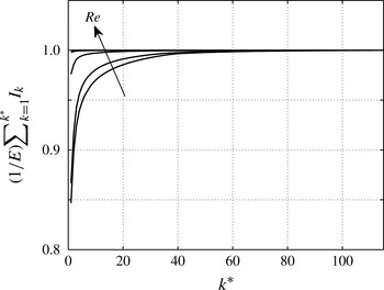
are computed with the full set of optimal and sub-optimals, which is computationally tractable in the case of inlet forcing since their number is equal to the number of degrees of freedom at the inlet. The effect of taking a limited number of sub-optimals is reported in appendix C. Note that although evaluating
 $E$
and
 $\boldsymbol{{\rm\nabla}}_{\ast }E$
is relatively costly, computations are largely parallelisable since different frequencies can be treated independently.
4. Harmonic response
In this section we present results about the response of the flow to small-amplitude harmonic forcing. Although the focus of this paper is on stochastic forcing at the inlet of the domain as a realistic model of random perturbations advected by the flow, we mention here harmonic forcing since it is a building block of the stochastic problem, and forcing in the volume for comparison purposes. The configuration
 ${\it\Gamma}=0.5$
,
 $\mathit{Re}=500$
, is considered unless otherwise stated.
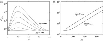
Figure 3(a) shows the optimal harmonic gain for inlet forcing
 $G_{in,1}$
for
 ${\it\Gamma}=0.5$
. The maximal optimal gain increases from 6.33 at
 $\mathit{Re}=100$
to
 $5.83\times 10^{3}$
at
 $\mathit{Re}=600$
, the optimal frequency being close to
 ${\it\omega}_{0}=0.5$
for all investigated Reynolds numbers. The dependence of the maximal optimal gain on Reynolds number is exponential beyond some value of
 $\mathit{Re}$
, as illustrated in figure 3(b), with
 $\log (\max _{{\it\omega}}G_{in,1})$
and
 $\log (\max _{{\it\omega}}G_{vol,1})$
scaling like
 $0.66\times 10^{-2}\mathit{Re}$
. The exponent for volume forcing was
 $\simeq 0.6\times 10^{-2}\mathit{Re}$
in the flow past a wall-mounted bump with
 $\mathit{Re}$
based on the bump height (Boujo et al.
Reference Boujo, Ehrenstein and Gallaire2013). This exponential dependence contrasts with parallel flows, where the maximal optimal harmonic gain only increases like
 $\mathit{Re}^{2}$
(Schmid & Henningson Reference Schmid and Henningson2001).
(a) Optimal harmonic gain for inlet forcing.
 ${\it\Gamma}=0.5$
,
 $\mathit{Re}=100,200,\dots ,600$
. (b) Maximum harmonic gain for volume and inlet forcing.
 ${\it\Gamma}=0.5$
.

Cantwell, Barkley & Blackburn (Reference Cantwell, Barkley and Blackburn2010) observed the same phenomenon for the maximal transient growth in several wall-bounded separated flows: they reported exponential dependence on
 $\mathit{Re}$
with exponent of order
 $10^{-2}$
(
 $0.45\times 10^{-2}$
for a sudden axisymmetric expansion,
 $0.61\times 10^{-2}$
for a stenotic flow, and
 $1.18\times 10^{-2}$
for the
 ${\it\Gamma}=0.5$
backward-facing step with
 $\mathit{Re}$
based on the centreline velocity), while in parallel flows the maximal transient growth only increases like
 $\mathit{Re}^{2}$
(Schmid & Henningson Reference Schmid and Henningson2001).
In these two analyses (harmonic response and transient growth), the spatial growth of perturbations is involved. In spatially developing flows, convective non-normality allows for an exponential growth over the entire shear layer length
 $l$
. Since the latter scales like
 $l={\it\alpha}\mathit{Re}$
, perturbations grow like
 $\text{exp}({\it\alpha}\mathit{Re})$
, with
 ${\it\alpha}$
a constant. In contrast, in parallel flows, component-type non-normality (e.g. lift-up and Orr mechanisms) results in algebraic growth, scaling like
 $\mathit{Re}^{2}$
as can be shown by considering the Orr–Sommerfeld–Squire equations (Schmid & Henningson Reference Schmid and Henningson2001) or a simple model thereof (Cossu Reference Cossu2014).
Focusing on
 $\mathit{Re}=500$
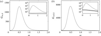
from now on, we compare the optimal harmonic gain for inlet forcing and volume forcing in figure 4. The gain is larger in the case of volume forcing, which is a consequence (i) of the choice of the norm used to measure forcing amplitude (two-dimensional versus one-dimensional), and (ii) of the greater efficiency with which two-dimensional forcing structures (allowed to occupy the whole domain) excite the flow, compared to one-dimensional forcing structures (restricted to the inlet). The maximum gain is
 $\max _{{\it\omega}}G_{in,1}=1.29\times 10^{3}$
at
 ${\it\omega}_{0}=0.49$
for inlet forcing, and
 $\max _{{\it\omega}}G_{vol,1}=7.46\times 10^{3}$
at
 ${\it\omega}_{0}=0.48$
for volume forcing. The latter values are in excellent agreement with those reported by Marquet & Sipp (Reference Marquet, Sipp, Schlatter and Henningson2010):
 $\max _{{\it\omega}}G_{vol,1}=7.5\times 10^{3}$
at
 ${\it\omega}_{0}=0.47$
. Sub-optimal branches in figure 4 have a much lower gain and mainly correspond to advection and diffusion. As pointed out by Marquet & Sipp (Reference Marquet, Sipp, Schlatter and Henningson2010), the flow response should therefore be dominated by the optimal response. Boujo et al. (Reference Boujo, Ehrenstein and Gallaire2013) observed this behaviour in a direct numerical simulation of a different geometry, with a predominance of the optimal response at optimal frequency. As discussed later in § 5, the sensitivity of the stochastic gain is also dominated by the sensitivity of the optimal harmonic gain at the optimal frequency.
Optimal harmonic gain for (a) inlet and (b) volume forcing.
 ${\it\Gamma}=0.5$
,
 $\mathit{Re}=500$
. Insets show the optimal gain and a few sub-optimal gains in logarithmic scale.

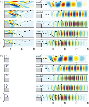
The optimal forcing and response are shown in figure 5 for different frequencies. They have a shorter wavelength as
 ${\it\omega}$
increases, consistent with most studies of harmonic optimal gain in convective flows (Alizard et al.
Reference Alizard, Cherubini and Robinet2009; Boujo et al.
Reference Boujo, Ehrenstein and Gallaire2013; Dergham et al.
Reference Dergham, Sipp and Robinet2013; Garnaud et al.
Reference Garnaud, Lesshafft, Schmid and Huerre2013). The volume optimal forcing is maximal close to the step corner for all frequencies. The optimal response is maximal downstream of the step corner: close to the upper reattachment point at
 ${\it\omega}=0.1$
, farther downstream as
 ${\it\omega}$
increases towards the optimal frequency
 ${\it\omega}_{0}\simeq 0.5$
, then farther upstream as frequency continues to increase. Interestingly, the optimal inlet forcing
 $\boldsymbol{f}_{in,1}(y)$
in figure 5(b) is very similar to the profile of optimal volume forcing in figure 5(a) close to the inlet
 $\boldsymbol{f}_{vol,1}(x\rightarrow -L_{in}^{+},y)$
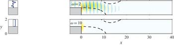
. Furthermore, these optimal inlet and volume forcings lead to very similar optimal responses (except for slight differences best seen at low frequency near the step corner and the lower recirculation region). Garnaud et al. (Reference Garnaud, Lesshafft, Schmid and Huerre2013) observed the same phenomenon over a broad range of frequencies. At higher frequencies, where amplification is small, the optimal inlet forcing tends to a plug profile and the response is concentrated at the step corner (figure 6).
Optimal harmonic forcing (left: real part of streamwise component
 $\boldsymbol{f}_{1}\boldsymbol{\cdot }\boldsymbol{e}_{x}$
) and optimal harmonic response (right: real part of cross-stream component
 $v_{1}$
): (a) volume forcing and corresponding response, (b) inlet forcing and corresponding response.
 ${\it\Gamma}=0.5$
,
 $\mathit{Re}=500$
.

Same as figure 5(b) but at higher frequencies.

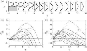
Interesting complementary information can be obtained from a local linear stability analysis, assuming the flow is parallel. At each streamwise location, the Orr–Sommerfeld equation was first solved for the temporal problem, the eigenvalue problem of the complex frequency
 ${\it\omega}^{(T)}$
for a given real streamwise wavenumber
 $k$
. We found at most one unstable eigenmode for all values of
 $x$
and
 $k$
. Next, the same Orr–Sommerfeld equation was solved for the spatial problem, the eigenvalue problem of the complex wavenumber
 $k^{(S)}$
for a given real frequency
 ${\it\omega}$
. The identification of the correct eigenvalue in the spatial problem is difficult in general. In order to make this process easier, Gaster’s relation
 $-k_{i}^{(S)}={\it\omega}_{i}^{(T)}/c_{g}$
(Gaster Reference Gaster1962) was used to estimate the spatial growth rate
 $-k_{i}^{(S)}$
from the available temporal growth rate
 ${\it\omega}_{i}^{(T)}$
and group velocity
 $c_{g}=\partial {\it\omega}_{r}^{(T)}/\partial k_{r}^{(T)}$
, close to the neutral curve where
 $k_{i}^{(S)}={\it\omega}_{i}^{(T)}=0$
. The eigenvalue of interest was then identified and followed while varying
 ${\it\omega}$
. Figure 7 shows the temporal and spatial growth rates at several locations. The flow is unstable between
 $x=0$
and
 $x=27$
, which corresponds to the region where streamwise velocity profiles contain inflection points (figure 7
a). The temporal growth rate (figure 7
b) is monotonically decreasing with
 $x$
, as shear gradually weakens downstream; in contrast, the spatial growth rate (figure 7
c) is also globally decreasing with
 $x$
but not monotonically at all frequencies, consistent with results from Kaiktsis et al. (Reference Kaiktsis, Karniadakis and Orszag1996) for similar geometry and flow conditions (
 ${\it\Gamma}\simeq 0.49$
,
 $\mathit{Re}\simeq 510$
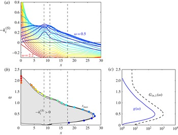
). This is best seen in figure 8(a), showing that
 $-k_{i}^{(S)}(x)$
has a local maximum around
 $x\simeq 9{-}11$
, i.e. between the upper separation and the lower reattachment. The spatially unstable domain in the
 $x{-}{\it\omega}$
plane is summarised in figure 8(b). As frequency increases, the unstable region quickly widens, from
 $x\simeq 9{-}11$
at
 ${\it\omega}=0$
, to a long region extending downstream up to
 $x=27$
at
 ${\it\omega}=0.5$
, before shrinking back towards the step corner
 $x=0$
, until the flow finally becomes stable everywhere for high frequencies
 ${\it\omega}\geqslant 2.2$
. The downstream neutral curve
 $-k_{i}^{(S)}=0$
is followed closely by the location
 $x_{max}$
where the energy density of the global optimal harmonic response is maximal,
 $$\begin{eqnarray}x_{max}=\arg \max _{x}\int \Vert \boldsymbol{u}_{1}(x,y)\Vert _{2}^{2}\text{d}y,\end{eqnarray}$$
consistent with the idea that perturbations grow spatially as long as
 $-k_{i}^{(S)}>0$
, and then decay. This is also reminiscent of the observation from Sipp & Marquet (Reference Sipp and Marquet2013) in a flat-plate boundary layer, where the optimal response shows a peak at
 $x_{max}$
close to the downstream neutral curve obtained from local stability analysis.
(a) Profiles of streamwise velocity for
 ${\it\Gamma}=0.5$
,
 $\mathit{Re}=500$
, with inflection points shown as dots. (b) Temporal and (c) spatial growth rates obtained from local stability analysis.

Local stability analysis for
 ${\it\Gamma}=0.5$
,
 $\mathit{Re}=500$
. (a) Streamwise evolution of the spatial growth rate
 $-k_{i}^{(S)}$
at different frequencies. (b) Region of local instability
 $-k_{i}^{(S)}>0$
(shaded area) and location of the maximum of the optimal response energy density
 $x_{max}$
(solid line and symbols). (c) Integral amplification factor
 $g$
(solid line) and optimal harmonic gain
 $G_{in,1}$
(dashed line, reproduced from figure 4
a). The thick line in (a) corresponds to the most amplified frequency
 ${\it\omega}=0.5$
.

One can quantify more precisely how much perturbations are amplified as they propagate downstream. To this end, we compute for each frequency the integral amplification factor
 $$\begin{eqnarray}g({\it\omega})=\exp \left(\int -k_{i}^{(S)}({\it\omega},x)\text{d}x\right)\end{eqnarray}$$
over the unstable region where
 $-k_{i}^{(S)}({\it\omega})>0$
. The integral amplification factor shown in figure 8(c) (solid line) is maximum close to
 ${\it\omega}=0.5$
. This is in very good agreement with the global optimal harmonic gain
 $G_{in,1}({\it\omega})$
(dashed line), also shown for qualitative comparison. Note that in this local analysis,
 ${\it\omega}=0.5$
is not the most unstable frequency at all locations: high frequencies display a much larger growth rate close to the step, as seen in figure 8(a); however, perturbations at
 ${\it\omega}=0.5$
do show the largest growth rate further downstream and take advantage of the longest possible unstable region, resulting in the largest integral amplification factor. The shapes of
 $g({\it\omega})$
and
 $G_{in,1}({\it\omega})$
are similar, too, except for
 ${\it\omega}\gtrsim 2$
; in this frequency range the parallel flow is locally stable, whereas in the global flow non-parallel effects and component-type non-normality (e.g. Orr mechanism) are at work. Overall, figure 8(b,c) indicates that the agreement between local and global stability analyses is remarkable, both in terms of instability/amplification region and in terms of most amplified frequency. Note also that Blackburn et al. (Reference Blackburn, Barkley and Sherwin2008) obtained a maximum mean perturbation energy at
 $x=26{-}27$
in two- and three-dimensional calculations, both in the optimal perturbations obtained from transient growth analysis and in a direct numerical simulation forced with small-amplitude perturbations (Gaussian white noise) at the inlet; this is consistent with Kaiktsis et al. (Reference Kaiktsis, Karniadakis and Orszag1996) and in very good agreement with our spatial and global analyses.
It is worth comparing further the results of the present harmonic response analysis with those of the transient growth analysis of Blackburn et al. (Reference Blackburn, Barkley and Sherwin2008). These authors reported a centre frequency
 ${\it\omega}=0.55$
in the spectral density of their forced three-dimensional direct numerical simulation, close to the most amplified frequency obtained in our harmonic response analysis. This frequency was identical to that of wave packets of streamwise wavelength 3.73 (measured in optimal perturbations from transient growth analysis) advected at the mean downstream channel velocity
 $U_{\infty }/3$
. Finally, the optimal initial perturbation in their transient growth analysis is strikingly similar to our optimal harmonic volume forcing at
 ${\it\omega}=0.5$
(figure 5
a). Although responses to initial perturbations, to sustained harmonic forcing and to sustained white noise are three different processes, the above-mentioned similarities point to the close relationship between the physical amplification phenomena involved in these processes.
5. Sensitivity and control of harmonic and stochastic amplification
As shown in § 4, the backward-facing step flow is a strong amplifier, with a potential for large amplification of harmonic and stochastic forcing. The objective of this section is to investigate how this amplification can be reduced by steady control. We stress that forcing is considered as an external perturbation, generally unwanted, whereas control is applied on purpose with the aim of reducing the amplification of the forcing. Hereafter, forcing at the inlet is considered.
We use the method presented in § 2.3 to compute the sensitivity of the optimal harmonic/stochastic gain to steady flow modification and steady control. Sensitivity maps provide quantitative and qualitative information (sensitivity values, regions of largest sensitivity) that are useful to design efficient control configurations in the volume (§ 5.1) or at the wall (§ 5.2).
5.1. Volume control
5.1.1. Flow modification
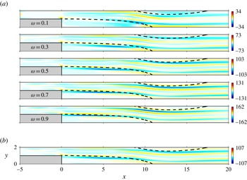
Figure 9 shows sensitivities to base-flow modification in the streamwise direction: regions of positive (respectively negative) sensitivity indicate where a small-amplitude increase of streamwise velocity would increase (respectively decrease) the gain. The optimal harmonic gain
 $G_{in,1}$
is most sensitive at the step corner, and in elongated regions parallel to the direction of the main flow (figure 9
a). The structure of these positive/negative sensitivity regions indicates that, for most frequencies, increasing shear in the shear layers near the boundaries of the upper/lower recirculation regions would result in a larger gain. Further downstream, increasing shear at the
 $y$
location of the base-flow inflection points would also result in a larger gain. This is consistent with the global amplification process being linked to the local shear instability mechanism. In contrast, some regions display a sensitivity which changes sign with
 ${\it\omega}$
, meaning that a modification of the base flow in such a region would increase
 $G_{in,1}$
at some frequencies and decrease it at others. Boujo et al. (Reference Boujo, Ehrenstein and Gallaire2013) made the same observation for the flow past a wall-mounted bump, and empirically proposed to design their control based on the optimal frequency alone. This approach appears justified for the present
 ${\it\Gamma}{-}\mathit{Re}$
conditions since the sensitivity of the stochastic gain
 $E$
(figure 9
b) is essentially similar to that of
 $G_{in,1}$
at the optimal frequency
 ${\it\omega}_{0}=0.5$
. Therefore, reducing the response to stochastic forcing is tantamount to reducing the optimal harmonic gain at the optimal frequency, which brings substantial benefits in terms of simplicity and computational cost.
Sensitivity of (a) optimal harmonic gain (
 $\boldsymbol{{\rm\nabla}}_{U}G_{in,1}^{2}/G_{in,1}^{2}$
) and (b) stochastic gain (
 $\boldsymbol{{\rm\nabla}}_{U}E/E$
) to base-flow modification (streamwise component
 $\boldsymbol{{\rm\nabla}}_{U}=\boldsymbol{e}_{x}\boldsymbol{\cdot }\boldsymbol{{\rm\nabla}}_{\boldsymbol{U}}$
).
 ${\it\Gamma}=0.5$
,
 $\mathit{Re}=500$
.

5.1.2. Volume control
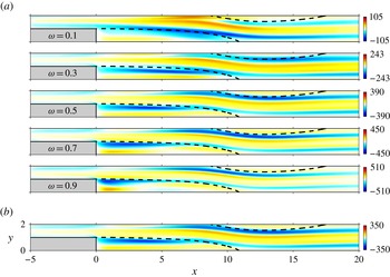
Figure 10 shows in the same way sensitivities to streamwise volume control: regions of positive (respectively negative) sensitivity indicate where a small-amplitude body force pointing in the
 $+x$
direction would increase (respectively decrease) the gain. Again, elongated regions of large sensitivity are found along the shear layers, but also in the lower recirculation zone, while the step corner is less sensitive. For the optimal harmonic gain (figure 10
a), variations with
 ${\it\omega}$
are still present, for instance near the upper wall upstream of the upper separation point. In this case too, the stochastic gain exhibits a sensitivity (figure 10
b) dominated by that of the optimal harmonic gain at the optimal frequency.
Sensitivity of (a) optimal harmonic gain (
 $\boldsymbol{{\rm\nabla}}_{C_{x}}G_{in,1}^{2}/G_{in,1}^{2}$
) and (b) stochastic gain (
 $\boldsymbol{{\rm\nabla}}_{C_{x}}E/E$
) to volume control (streamwise component
 $\boldsymbol{{\rm\nabla}}_{C_{x}}=\boldsymbol{e}_{x}\boldsymbol{\cdot }\boldsymbol{{\rm\nabla}}_{\boldsymbol{C}}$
).
 ${\it\Gamma}=0.5$
,
 $\mathit{Re}=500$
.

5.1.3. Control cylinder
In practice, it is difficult to generate arbitrary volume forces in the flow. It is more common, both experimentally and numerically, to use open-loop devices to control, for instance, aerodynamic forces or vortex shedding (Strykowski & Sreenivasan Reference Strykowski and Sreenivasan1990; Igarashi Reference Igarashi1997; Dalton, Xu & Owen Reference Dalton, Xu and Owen2001; Mittal & Raghuvanshi Reference Mittal and Raghuvanshi2001; Cadot, Thiria & Beaudoin Reference Cadot, Thiria, Beaudoin, Braza and Hourigan2009; Parezanović & Cadot Reference Parezanović and Cadot2009, Reference Parezanović and Cadot2012). Sensitivity analysis is well suited to estimating the effect of a wire, i.e. a small control cylinder of diameter
 $d$
, using (i) the sensitivity to volume forcing already computed, and (ii) a simple model for the control force
 $\boldsymbol{C}$
exerted by the cylinder on the flow, namely a force opposite to the drag felt by the control cylinder in a steady uniform flow at the local velocity
 $\boldsymbol{U}_{b}(x,y)$
(Hill Reference Hill1992; Marquet et al.
Reference Marquet, Sipp and Jacquin2008; Meliga et al.
Reference Meliga, Sipp and Chomaz2010; Pralits, Brandt & Giannetti Reference Pralits, Brandt and Giannetti2010; Fani, Camarri & Salvetti Reference Fani, Camarri and Salvetti2012):
 ${\bf\delta}\boldsymbol{C}(x,y)=-(1/2)dC_{d}(x,y)\Vert \boldsymbol{U}_{b}(x,y)\Vert \boldsymbol{U}_{b}(x,y){\it\delta}(x-x_{c},y-y_{c})$
, where
 ${\it\delta}$
is the two-dimensional Dirac delta function, and the drag coefficient
 $C_{d}$
depends on the local Reynolds number
 $\mathit{Re}_{d}(x,y)=\Vert \boldsymbol{U}_{b}(x,y)\Vert d/{\it\nu}$
. Here we choose
 $d=0.05$
, corresponding to Reynolds numbers
 $\mathit{Re}_{d}\leqslant 25$
everywhere in the flow. We therefore use the following composite expression for the drag coefficient:
 $$\begin{eqnarray}\displaystyle & 0.5\leqslant \mathit{Re}_{d}\leqslant 25:\quad C_{d}=a+b\mathit{Re}_{d}^{c},\quad a=0.85,\ b=10.6,\ c=-0.72, & \displaystyle\end{eqnarray}$$
 $$\begin{eqnarray}\displaystyle & \displaystyle \mathit{Re}_{d}\leqslant 0.5:\quad C_{d}=\frac{8{\rm\pi}}{\mathit{Re}_{d}S}\left(1-\frac{\mathit{Re}_{d}^{2}}{32}\left(S-\frac{1}{2}+\frac{5}{16S}\right)\right), & \displaystyle\end{eqnarray}$$
 $S=(1/2)-{\it\gamma}-\log (\mathit{Re}_{d}/8)$
and
 ${\it\gamma}$
is Euler’s constant. Expression (5.1) is a fit of experimental data from Tritton (Reference Tritton1959) and in-house numerical results, while (5.2) is an extension of Oseen’s formula
 $C_{d}=8{\rm\pi}/\mathit{Re}_{d}S$
for low Reynolds numbers (Oseen Reference Oseen1910; Proudman & Pearson Reference Proudman and Pearson1957) derived by Tomotika & Aoi (Reference Tomotika and Aoi1951). In practice, the exact value at low Reynolds number is of little importance: although the drag coefficient goes to infinity like
 ${\sim}1/(\mathit{Re}_{d}\log \mathit{Re}_{d})$
as
 $\mathit{Re}_{d}\rightarrow 0$
as an artificial consequence of the aerodynamic definition of
 $C_{d}$
, the actual force exerted on the cylinder goes to zero like
 ${\sim}\mathit{Re}_{d}/\log \mathit{Re}_{d}$
.
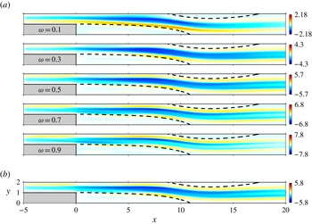
The effect of a small control cylinder is shown in figure 11. The amplification of stochastic noise is best reduced when inserting the control cylinder in an elongated region extending from the step to the upper reattachment point, where the main-stream velocity is large. Conversely, noise amplification increases when the control cylinder is inserted in the outer vicinity of recirculation regions, where shear is large. Again, the basic mechanism is shear strengthening (respectively shear weakening) due to the cylinder wake in the main stream (respectively in the shear layers). Recirculation regions themselves have no significant effect as a result of their low velocities.
Effect of a small control cylinder of diameter
 $d=0.05$
on (a) optimal harmonic gain (
 ${\it\delta}G_{in,1}^{2}/G_{in,1}^{2}$
) and (b) stochastic gain (
 ${\it\delta}E/E$
).
 ${\it\Gamma}=0.5$
,
 $\mathit{Re}=500$
.

5.2. Wall control
5.2.1. Sensitivity maps
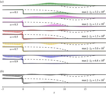
Sensitivities to wall control are shown in figure 12. Arrows point in the direction of positive sensitivity: at each point of the wall, blowing or suction in the direction of the corresponding arrow would increase the gain. More generally, an actuation direction whose scalar product with the sensitivity is positive would increase the gain, while an actuation direction orthogonal to the sensitivity would have no first-order effect. The sensitivity of the harmonic optimal gain (figure 12
a) is essentially normal to the wall and, again, changes sign with frequency, except notably at the lower wall of the inlet channel. The sensitivity of the stochastic gain (figure 12
b), once again mostly dominated by that of the optimal harmonic gain at the optimal frequency, is maximum just upstream of the step corner. Given the sign of the sensitivity, wall suction at this location should reduce noise amplification. Note that the step corner is often chosen for wall control in this flow and similar ones (Pastoor et al.
Reference Pastoor, King, Noack and Tadmor2005; Beaudoin et al.
Reference Beaudoin, Cadot, Aider and Wesfreid2006; Henning & King Reference Henning and King2007; Hervé et al.
Reference Hervé, Sipp, Schmid and Samuelides2012), but other locations have a sensitivity of comparable magnitude, like the vertical wall (where blowing should reduce
 $E$
) and the upper wall of the inlet channel (where suction should reduce
 $E$
). These locations could offer interesting alternatives to the step corner depending on technical feasibility constraints.
Sensitivity to wall control of (a) the optimal harmonic gain (
 $\boldsymbol{{\rm\nabla}}_{\boldsymbol{U}_{c}}G_{in,1}^{2}$
) and (b) the stochastic gain (
 $\boldsymbol{{\rm\nabla}}_{\boldsymbol{U}_{c}}E$
).
 ${\it\Gamma}=0.5$
,
 $\mathit{Re}=500$
. Arrows point in the direction of positive sensitivity (i.e. increasing gain).

5.2.2. Validation
We illustrate the effect of steady wall control on the harmonic/stochastic gain, and use this opportunity to validate the sensitivity analysis. We consider several locations upstream and downstream of the step corner, both at the lower and upper walls, as represented in figure 13(a). For the sake of simplicity, and since we observed that sensitivity to wall-normal control was much larger than that of tangential control, we use blowing and suction in the normal direction only. We choose Gaussian actuation profiles
 $V_{c}(x)=(-\boldsymbol{n}\boldsymbol{\cdot }\boldsymbol{e}_{y})\,W\exp (-(x-x_{c})^{2}/{\it\sigma}_{c}^{2})/({\it\sigma}_{c}\sqrt{{\rm\pi}})$
for control on horizontal walls, and
 $U_{c}(y)=(-\boldsymbol{n}\boldsymbol{\cdot }\boldsymbol{e}_{x})\,W\exp (-(y-y_{c})^{2}/{\it\sigma}_{c}^{2})/({\it\sigma}_{c}\sqrt{{\rm\pi}})$
for control on the vertical wall, with characteristic width
 ${\it\sigma}_{c}=0.1$
and flow rate
 $W$
, positive for blowing and negative for suction (recall that
 $\boldsymbol{n}$
points outward). We compare results from full gain calculations for flows actually controlled with the Gaussian actuation profile applied as a boundary condition, and predictions from sensitivity analysis according to (2.13)–(2.16), i.e.
 ${\it\delta}G_{in,k}^{2}=(\boldsymbol{{\rm\nabla}}_{\boldsymbol{U}_{c}}G_{in,k}^{2}\mid {\bf\delta}\boldsymbol{U}_{c})$
and
 ${\it\delta}E=(\boldsymbol{{\rm\nabla}}_{\boldsymbol{U}_{c}}E\mid {\bf\delta}\boldsymbol{U}_{c})$
.
Wall control with steady Gaussian blowing/suction for
 ${\it\Gamma}=0.5$
,
 $\mathit{Re}=500$
. (a) Sketch of control configurations 1–5. Blowing corresponds to positive flow rates (
 $W>0$
), suction to negative flow rates (
 $W<0$
). (b) Variation of harmonic gain at
 ${\it\omega}=0.5$
with flow rate in configuration 4 (
 $x_{c}=-1$
,
 $y_{c}=2$
). (c) Overall optimal harmonic gain reduction in control configuration 4 with suction flow rate
 $W_{4}=-0.01$
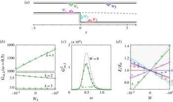
. (d) Variation of stochastic gain (normalised by its uncontrolled value) with flow rate. Solid lines show predictions from sensitivity analysis, symbols are actual results from controlled flows.

Figure 13(b) shows the effect of steady blowing and suction at the upper wall upstream of the step (configuration 4) on the optimal harmonic gain and the first two sub-optimal gains at the optimal frequency
 ${\it\omega}_{0}=0.5$
. Predictions from sensitivity analysis (solid lines) are in good agreement with full calculations (symbols), as could be expected for small control amplitudes (
 $W$
less than 0.01, to be compared to the inlet flow rate
 $2U_{\infty }h_{in}/3=2/3$
). The effect of wall suction on the optimal gain at other frequencies is shown in figure 13(c). As predicted by sensitivity (figure 12), the gain is reduced over the whole range of most amplified frequencies. Moving to the stochastic gain in figure 13(d), we observe a good agreement too: sensitivity analysis (solid line) captures well the reduction in
 $E$
from its uncontrolled value
 $E_{0}$
compared to actual results from full calculations (symbols). In some control configurations, the actual variation of
 $E$
departs from sensitivity predictions as the flow rate becomes larger, due to nonlinear effects not taken into account in the first-order linear sensitivity analysis based on the assumption of small-amplitude control. These nonlinear effects are larger in configurations 3 and 5, i.e. for wall actuation downstream of the step.
5.2.3. Towards passive wall actuation
Wall control allows us to choose the actuation direction (blowing or suction) and orientation (angle) freely. This is an advantage over volume control: typically, a small cylinder can only produce a force in the direction of the flow. The price to pay is a more complex actuation system and a potentially higher power requirement to drive the control, unless one takes advantage of pressure differences: connecting wall regions of relative higher and lower pressure with a small channel could induce natural suction and blowing at the inlet and at the outlet, respectively. This configuration would not require any mechanical device and would therefore constitute a means of passive control.
(a) Passive control by means of a channel connecting regions of high and low pressure (solid line). The induced flow results in wall suction at
 $A$
and wall blowing at
 $B$
, and reduces the stochastic response
 $E$
as predicted by the sensitivity to wall-normal actuation (the dash-dotted line shows the normal component, much larger than the tangential component as observed in figure 12). (b) Reduction in optimal harmonic gain for
 $x_{A}=-1$
,
 $y_{B}=0.75$
and channel height
 $h_{c}=0.15$
. Dash-dotted line: uncontrolled flow; solid line: estimation from (5.4) (Poiseuille flow concentrated at
 $A$
and
 $B$
); symbols joined with dashed lines: actual optimal harmonic gain for the flow with channel.

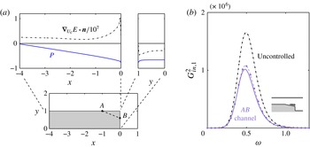
This could be implemented in the backward-facing step flow between the lower wall upstream of the corner (suction at higher pressure) and the vertical wall (blowing at lower pressure): figure 14(a) shows that pressure (solid line) along the horizontal wall is larger than on the vertical wall, and that the sign of the sensitivity of
 $E$
(dash-dotted line) is such that the stochastic gain can be reduced precisely with suction on the horizontal wall and blowing on the vertical wall.
A crude estimate of the expected reduction in
 $E$
can be obtained by assuming that connecting points
 $A$
and
 $B$
with coordinates
 $\boldsymbol{x}_{A}=(x_{A},h_{s})$
and
 $\boldsymbol{x}_{B}=(0,y_{B})$
with a straight channel would result in a fully developed plane Poiseuille flow of mean velocity
 $U_{m}=\mathit{Re}\,h_{c}^{2}\,{\rm\Delta}P/12l_{c}$
, where
 ${\rm\Delta}P=P_{A}-P_{B}$
is the pressure difference, and
 $h_{c}$
and
 $l_{c}=\sqrt{x_{A}^{2}+(h_{s}-y_{B})^{2}}$
are the channel height and length. Assuming further that at both ends the induced flow is localised at points
 $A$
and
 $B$
, the velocity vector is
 $$\begin{eqnarray}{\bf\delta}\boldsymbol{U}(\boldsymbol{x}_{A})={\bf\delta}\boldsymbol{U}(\boldsymbol{x}_{B})=U_{m}\left(\begin{array}{@{}c@{}}\cos {\it\theta}\\ -\text{sin}\;{\it\theta}\end{array}\right)=\frac{U_{m}}{l_{c}}\left(\begin{array}{@{}c@{}}|x_{A}|\\ h_{s}-y_{B}\end{array}\right),\end{eqnarray}$$
where
 ${\it\theta}>0$
is the angle between the channel axis and the horizontal
 $\boldsymbol{e}_{x}$
. Taking the inner product with the sensitivity yields the stochastic response reduction
 $$\begin{eqnarray}{\it\delta}E=\frac{\mathit{Re}\,h_{c}^{2}\,{\rm\Delta}P}{12l_{c}^{2}}\left(\boldsymbol{{\rm\nabla}}_{\boldsymbol{U}_{c}}E(\boldsymbol{x}_{A})+\boldsymbol{{\rm\nabla}}_{\boldsymbol{U}_{c}}E(\boldsymbol{x}_{B})\right)\boldsymbol{\cdot }\left(\begin{array}{@{}c@{}}|x_{A}|\\ h_{s}-y_{B}\end{array}\right),\end{eqnarray}$$
and a similar expression for harmonic gains
 $G_{k}^{2}({\it\omega})$
. This expression shows that there is a trade-off among pressure difference, channel length, channel angle, and sensitivity: for instance, choosing
 $A$
far upstream increases both
 ${\rm\Delta}P$
and
 $l_{c}$
, which have opposite effects on the channel velocity; similarly, choosing
 $A$
close to the step corner yields a larger sensitivity but also increases unfavourably the angle
 ${\it\theta}$
between the control jet and the wall normal in
 $B$
.
Figure 14(b) shows the reduction in optimal harmonic gain for
 $x_{A}=-1,y_{B}=0.75$
and
 $h_{c}=0.15$
, as estimated with (5.4) from geometry, pressure and sensitivity information only (solid line), and as obtained from the controlled nonlinear flow with the channel included in the computational mesh (symbols). In spite of strongly simplifying assumptions, the estimated reduction has the correct order of magnitude. Note that the channel velocity
 $U_{m}$
scales like
 $h_{c}^{2}$
, thus only a limited benefit can be expected when using narrow channels.
6. Discussion
The analysis of § 5 for
 ${\it\Gamma}=0.5$
,
 $\mathit{Re}=500$
showed that the sensitivity of the stochastic gain was very similar to the sensitivity of the optimal harmonic gain at the optimal frequency
 ${\it\omega}_{0}$
. One can therefore reduce noise amplification using a steady volume or wall control configuration which reduces the amplification of harmonic forcing at
 ${\it\omega}_{0}$
. This a posteriori observation implies that summation over frequencies and sub-optimals is not required in practice to predict the effect of steady control.
In this section, we investigate the following two aspects: (i) whether one can get an a priori hint about the effect of steady control on the stochastic gain from the sensitivity of an alternative scalar quantity, the recirculation length; (ii) whether the optimal harmonic response at
 ${\it\omega}_{0}$
still dominates in different
 ${\it\Gamma}{-}\mathit{Re}$
configurations.
6.1. Recirculation length
In many flows, the length of the recirculation region is related to stability properties. It increases with Reynolds number as long as the flow is steady, while its mean value decreases when the flow becomes unsteady (Sinha, Gupta & Oberai Reference Sinha, Gupta and Oberai1981; Armaly et al. Reference Armaly, Durst, Pereira and Schönung1983) as a consequence of mean-flow corrections induced by Reynolds stresses. Due to the presence of the recirculation region, a shear layer forms, adjacent to the separatrix, which drives the strong convective inviscid instability underpinning the large harmonic/stochastic amplification, as detailed in § 4.
In this context, it is natural to investigate whether there exists any relationship between recirculation length and stochastic gain when steady control is applied to the flow. To this end, we focus on steady wall control, and compute the effect of blowing/suction at the upstream channel walls (configurations 1 and 4 in figure 13
a) on the length of the lower recirculation region
 $l_{l}=x_{lr}$
, and the length of the upper recirculation region
 $l_{u}=x_{ur}-x_{us}$
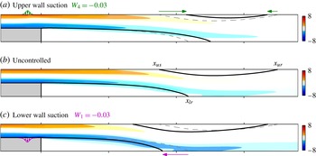
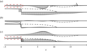
. Figure 15 shows vorticity contours in the controlled and uncontrolled flows. Upper-wall suction (figure 15
a) deflects the main flow upwards, which moves the upper separation and lower reattachment points downstream (compare dashed and solid separatrices without and with control). As a result, the recirculation region on the upper wall is shortened while that on the lower wall is lengthened. Conversely, lower-wall suction (figure 15
c) deflects the main flow downwards, which moves the upper separation and lower reattachment points upstream, resulting in a shorter recirculation region on the lower wall and a longer one on the upper wall.
Effect of steady wall actuation: wall-normal suction at the upstream (a) upper or (c) lower wall shortens the recirculation region at the upper or lower wall, respectively, compared to the (b) uncontrolled flow whose separatrices are shown as thin dashed lines in (a) and (c). Contours show spanwise vorticity
 $\partial _{x}V-\partial _{y}U$
.
 ${\it\Gamma}=0.5$
,
 $\mathit{Re}=500$
.

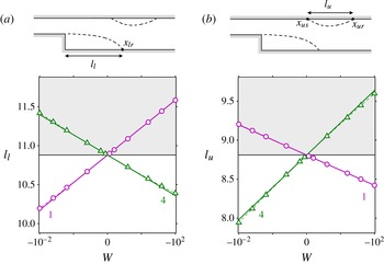
Figure 16 shows the variation in lower and upper recirculation length with control flow rate. Relatively small control flow rates have a significant impact on both recirculation lengths:
 $|{\it\delta}l|\simeq 5{-}10\,\%$
for
 $|W|=0.01$
. Applying sensitivity analysis to the recirculation lengths (Boujo & Gallaire Reference Boujo and Gallaire2014a
,Reference Boujo and Gallaire
b
), we find that variations are almost linear in this range of flow rates: nonlinear results from full Navier–Stokes calculations (symbols) closely follow predictions from sensitivity analysis (lines).
Variation of (a) lower and (b) upper recirculation lengths with steady wall blowing/suction flow rate (configurations 1 and 4 shown in figure 13). Solid lines show predictions from sensitivity analysis, symbols joined with dashed lines are actual results from controlled flows.
 ${\it\Gamma}=0.5$
,
 $\mathit{Re}=500$
.

Figure 17 shows the sensitivity of the recirculation lengths to wall control. The upper recirculation region (figure 17
a) is most effectively shortened using wall suction on the upper wall upstream of
 $x_{us}$
, or wall blowing on the vertical wall and the lower wall downstream of the step. The sensitivity of the lower recirculation region (figure 17
c) has a similar distribution but the opposite sign almost everywhere, indicating that any wall control has opposite effects on
 $l_{u}$
and
 $l_{l}$
. As a side note, the sensitivity of
 $l_{u}$
is very large in the vicinity of
 $x_{us}$
and
 $x_{ur}$
, and the sensitivity of
 $l_{l}$
is very large in the vicinity of
 $x_{lr}$
.
Sensitivity to wall control of (a) the upper recirculation length (
 $\boldsymbol{{\rm\nabla}}_{\boldsymbol{U}_{c}}l_{u}$
), (b) the stochastic gain (
 $\boldsymbol{{\rm\nabla}}_{\boldsymbol{U}_{c}}E$
) (reproduced from figure 12
b) and (c) the lower recirculation length (
 $\boldsymbol{{\rm\nabla}}_{\boldsymbol{U}_{c}}l_{l}$
).
 ${\it\Gamma}=0.5$
,
 $\mathit{Re}=500$
. Arrows point in the direction of positive sensitivity (i.e. increasing lengths and gain).

If we now compare these two sensitivity maps to that of the stochastic gain (figure 17
b, reproduced from figure 12
b), overall distributions are different, and it seems unlikely at first sight that considerations about recirculation lengths can guide the design of a simple wall control configuration aiming at reducing noise amplification. However, if we focus on the upstream channel (
 $x<0$
) it appears that
 $E$
and
 $l_{u}$
(respectively
 $l_{l}$
) have sensitivities of the same sign on the upper (respectively lower) walls. This suggests that if
 $E$
is to be reduced with wall control in the upstream channel, one can use wall control on the upper wall and aim at shortening the upper recirculation region, or use wall control on the lower wall and aim at shortening the lower recirculation region.
6.2. On the predominance of the optimal harmonic response
We observed in § 5 that for
 ${\it\Gamma}=0.5$
,
 $\mathit{Re}=500$
the sensitivity of the stochastic gain
 $E$
was very similar to that of the optimal gain
 $G_{in,1}$
at the optimal frequency
 ${\it\omega}_{0}$
. In order to test the robustness of this observation, we now consider two other configurations where the sensitivity of
 $E$
is more likely to differ from the sensitivity of
 $G_{in,1}({\it\omega}_{0})$
. In the first configuration we keep the same geometry (
 ${\it\Gamma}=0.5$
) but decrease the Reynolds number to
 $\mathit{Re}=200$
; in the second one we use a smaller step with expansion ratio
 ${\it\Gamma}=0.3$
at the stable Reynolds number
 $\mathit{Re}=2800$
(recall that
 $\mathit{Re}_{c}>2900$
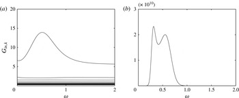
for this expansion ratio, as mentioned in § 3). From the harmonic gains shown in figure 18 we can make the following remarks: (i) reducing the Reynolds number makes the peak of
 $G_{in,1}$
less marked, thus possibly increasing the relative importance of frequencies other than the optimal one, as well as the importance of sub-optimal forcings relative to the optimal one; (ii) a double peak appears when reducing the step height, which might result in contributions of equal importance from two well-separated frequencies (
 ${\it\omega}_{0}=0.31$
and
 ${\it\omega}_{0}^{\prime }=0.55$
in the present case).
Optimal harmonic gain and sub-optimal gains for inlet forcing. (a)
 ${\it\Gamma}=0.5,\mathit{Re}=200$
, (b)
 ${\it\Gamma}=0.3,\mathit{Re}=2800$
.

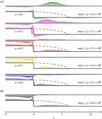
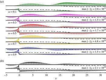
Figures 19 and 20 show sensitivities to wall control for these two configurations. Although slight differences can be noticed, the stochastic gain still has a sensitivity largely dominated by the sensitivity of the optimal harmonic gain at the optimal frequency
 ${\it\omega}_{0}$
. In particular, locations of maximal sensitivity of
 $E$
are captured robustly by the sensitivity of
 $G_{in,1}({\it\omega}_{0})$
. Therefore, even though integrating over a range of frequencies (i.e. performing a weighted average) should have a smoothing effect, the net result is almost unaffected by frequencies far from the optimal one. Close inspection shows that all sensitivity fields (for base-flow modification, volume control and wall control) change continuously with
 ${\it\omega}$
around the optimal frequency, and slowly enough for their integral to be eventually dominated by
 $\boldsymbol{{\rm\nabla}}_{\ast }G_{in,1}^{2}({\it\omega}_{0})$
. For instance, the two distinct peaks in
 $G_{in,1}$
for
 ${\it\Gamma}=0.3$
,
 $\mathit{Re}=2800$
(figure 18
b), are actually associated with very similar sensitivity fields. In addition, sub-optimals appear to contribute only little. This is not surprising for
 ${\it\Gamma}=0.5$
,
 $\mathit{Re}=500$
, since sub-optimal gains
 $G_{k}$
for
 $k\geqslant 2$
are smaller than
 $G_{1}$
by a factor of about two orders of magnitude in the range of most amplified frequencies (see figure 4). This is more surprising for
 ${\it\Gamma}=0.5$
,
 $\mathit{Re}=200$
, where this factor is reduced to approximately 5 (figure 18
a). We conclude that sub-optimals play a role only at even lower Reynolds numbers, where amplification mechanisms are weak anyway. Therefore, sensitivity analysis and steady control design can be conducted with good confidence on the optimal harmonic gain at the optimal frequency alone, rather than on the full stochastic response, thereby dramatically reducing the computational cost of the process.
Sensitivity of (a) optimal harmonic gain (
 $\boldsymbol{{\rm\nabla}}_{\boldsymbol{U}_{c}}G_{in,1}^{2}$
) and (b) stochastic gain (
 $\boldsymbol{{\rm\nabla}}_{\boldsymbol{U}_{c}}E$
) to wall control.
 ${\it\Gamma}=0.5$
,
 $\mathit{Re}=200$
.

Sensitivity of (a) optimal harmonic gain (
 $\boldsymbol{{\rm\nabla}}_{\boldsymbol{U}_{c}}G_{in,1}^{2}$
) and (b) stochastic gain (
 $\boldsymbol{{\rm\nabla}}_{\boldsymbol{U}_{c}}E$
) to wall control.
 ${\it\Gamma}=0.3$
,
 $\mathit{Re}=2800$
.

These observations are limited to the backward-facing step flow and to expansion ratios and Reynolds numbers investigated in this paper, although we believe they might bear generality in other strong amplifier flows. In flows where perturbations undergo large amplification in well-separated frequency ranges, the relationship among local stability, transient growth, and response to harmonic/stochastic forcing might be more subtle.
7. Conclusion
The response to time-harmonic and time-stochastic forcing in the two-dimensional flow past a backward-facing step was analysed. For the expansion ratio
 ${\it\Gamma}=0.5$
and Reynolds number
 $\mathit{Re}=500$
, a global linear stability analysis predicts that the flow is stable but a large amplification of both harmonic and stochastic forcing was observed, typical of noise amplifier flows. A local spatial stability analysis yielded very good agreement with global harmonic response, transient growth studies and direct numerical simulation, especially in terms of most amplified frequency (
 ${\it\omega}_{0}=0.5$
) and streamwise location of maximum response (
 $x\simeq 25{-}27$
).
Sensitivity analysis was used to study in a systematic way the effect of small-amplitude steady control in the volume or at the wall. A variational technique was used to derive analytical expressions for sensitivity, extending existing methods to stochastic forcing localised at the inlet. For volume forcing, sensitivity is classically computed from the forcing and corresponding response, while for inlet forcing it is found from the response and from an intermediate adjoint velocity field. In both cases, the sensitivity of the stochastic gain is expressed as a simple combination of sensitivities of optimal and sub-optimal harmonic gains over all frequencies.
Sensitivity maps obtained from this analysis allowed us, without computing any controlled flows, to identify most-sensitive regions where control can increase or decrease harmonic/stochastic gain the most efficiently. In particular, passive control by means of a small cylinder decreases the gain in the main stream downstream of the step, and increases the gain in the shear layers at the edges of the recirculation regions. Active control by means of wall blowing and suction is most effective on the vertical wall of the step and on the horizontal walls of the upstream channel.
For several Reynolds numbers and expansion ratios, it was observed that the sensitivity of the stochastic response was dominated to a large extent by the sensitivity of the optimal harmonic response at the most amplified frequency. This suggests that in this noise amplifier flow, and possibly in others, the design of open-loop control aiming at reducing noise amplification can be performed by targeting the optimal harmonic response at the optimal frequency only.
Possible extensions of the sensitivity analysis presented in this study include coloured noise, unsteady control and three-dimensional flows.
Acknowledgements
Unpublished work (Marquet, Sipp & Lesshafft Reference Marquet, Sipp and Lesshafft2010) dealing with the backward-facing step for
 ${\it\Gamma}=0.5$
,
 $\mathit{Re}=500$
, was brought to our attention during the reviewing process. We thank these authors for interesting information and stimulating discussions. We also wish to thank X. Garnaud, C. Arratia and E. Serre for their advice and comments, and the referees for valuable suggestions. This work was supported by the Swiss National Science Foundation (grant no. 200021-130315) and the French National Research Agency (project no. ANR-09-SYSC-001).
Optimal harmonic gain for (a) volume and (b) inlet forcing for different inlet lengths:
 $L_{in}=1$
(dashed line),
 $L_{in}=5$
(dash-dotted line) and
 $L_{in}=10$
(solid line). Insets show the convergence of the maximum gain value with increasing inlet length.
 ${\it\Gamma}=0.5$
,
 $\mathit{Re}=500$
.

Influence of inlet length (
 $L_{in}=1$
, 5 and 10 from top to bottom) on optimal harmonic forcing (left: real part of streamwise component
 $\boldsymbol{f}_{1}\boldsymbol{\cdot }\boldsymbol{e}_{x}$
) and optimal harmonic response (right: real part of cross-stream component
 $v_{1}$
): (a) volume forcing and corresponding response, (b) inlet forcing and corresponding response.
 ${\it\Gamma}=0.5$
,
 $\mathit{Re}=500$
,
 ${\it\omega}=0.5$
.

Stochastic gain
 $E$
versus
 $\mathit{Re}$
(solid lines) for cut-off frequencies
 ${\it\omega}_{c}=2$
(thick line) and
 ${\it\omega}_{c}=3$
, 5, 7, 10 (thin lines). The maximum harmonic optimal gain is also shown for reference (dashed line).

Appendix A. Influence of inlet length
Figures 21 and 22 show how the optimal harmonic gain, forcing and response depend on the inlet length. In the case of volume forcing (figure 21
a), the optimal gain
 $G_{vol,1}$
is not much affected by the inlet length, since the optimal forcing is well localised near the step corner and only a small amount of energy is introduced in the upstream inlet region. This is illustrated for
 ${\it\omega}=0.5$
in figure 22(a). In the case of inlet forcing (figure 21
b), the optimal gain varies significantly when the inlet length is increased up to
 $L_{in}\simeq 5$
, consistent with the observation of Garnaud et al. (Reference Garnaud, Lesshafft, Schmid and Huerre2013). Here
 $G_{in,1}$
decreases with
 $L_{in}$
due to viscous effects which smooth out perturbations when they enter the flow farther upstream of the step corner, i.e. upstream of the locally unstable region. Figure 22(b) shows that the optimal response keeps the same spatial structure although the inlet optimal forcing does vary with
 $L_{in}$
due to a phase effect (as mentioned in § 4, the inlet optimal forcing is similar to the profile of the volume optimal forcing close to
 $x=L_{in}^{+}$
, and here we fix the phase at
 $x=0$
,
 $y=1.5$
for all cases).
Convergence of the partial sum
 $\sum _{k}I_{k}$
(2.7) towards the full stochastic gain
 $E$
. Reynolds number
 $\mathit{Re}=100,200,\dots ,700$
.

Appendix B. Influence of cut-off frequency
Figure 23 shows the effect of the cut-off frequency in the integral evaluation of the stochastic response (see § 3). Increasing
 ${\it\omega}_{c}$
yields a slight increase in
 $E$
because the optimal harmonic gain
 $G_{in,1}({\it\omega})$
does not decrease to zero at large frequencies
 ${\it\omega}\geqslant 2$
but instead saturates to a finite value. However for large Reynolds numbers this finite value is negligible compared to the peak value
 $\max _{{\it\omega}}G_{in,1}$
at
 ${\it\omega}_{0}=0.5$
, and
 $E$
is unaffected by the exact value of the cut-off frequency provided
 ${\it\omega}_{c}$
is sufficiently larger than
 ${\it\omega}_{0}$
.
Appendix C. Influence of
 $k$
and
$\mathit{Re}$


As mentioned in §§ 5–6, the stochastic gain
 $E$
and its sensitivities
 $\boldsymbol{{\rm\nabla}}_{\ast }E$
are mainly influenced by optimal harmonic quantities
 $G_{1}^{2}$
and
 $\boldsymbol{{\rm\nabla}}_{\ast }G_{1}^{2}$
, especially at larger Reynolds numbers. Figure 24 quantifies this phenomenon. At
 $\mathit{Re}=300$
, the contribution from the optimal harmonic gain alone reaches more than 97 % of
 $E$
, while that of the first sub-optimal gain
 $k=2$
amounts to a mere 1 %. Even at a Reynolds number as low as
 $\mathit{Re}=100$
,
 $G_{in,1}$
contributes for 85 %,
 $G_{in,2}$
for 5 %, and 25 sub-optimals are enough to reach 99 % of
 $E$
.