1. Introduction
The atmospheric boundary layer (ABL) is often stably stratified at night, in polar regions or, in general, when relatively warm air is advected over a colder surface (Stull Reference Stull1988). This implies that the surface and adjacent lower air layers are colder and denser than the upper layers, related to an increase of potential temperature with height. As a result, vertical motions and turbulence are suppressed by buoyancy. Due to the relatively weak turbulence under stably stratified conditions, the complicated interaction with both large-scale forcings and small-scale phenomena, such as radiation, fog and dew formation, drainage flow, atmospheric subsidence, internal gravity waves, and low-level jets, becomes more important (Holtslag et al. Reference Holtslag2013). A particular feature of the stable atmospheric boundary layer is that the wind direction substantially changes with height as a consequence of Coriolis forces arising from the Earth’s rotation, also referred to as the Ekman layer. Moreover, the influence of even small local variations in surface properties such as topography, roughness or temperature, which may be less important under neutral or unstable conditions, can be substantial in stably stratified flows (McCabe & Brown Reference McCabe and Brown2007; Mahrt Reference Mahrt2014; Lee, Gohari & Sarkar Reference Lee, Gohari and Sarkar2020). To date, many aspects of the stable boundary layer (SBL) and non-uniform surface–flow interaction remain poorly understood, posing challenges on weather and climate modelling, as well as fluid-related engineering applications (Fernando & Weil Reference Fernando and Weil2010; Mahrt Reference Mahrt2014; Zonta & Soldati Reference Zonta and Soldati2018; Bou-Zeid et al. Reference Bou-Zeid, Anderson, Katul and Mahrt2020; Couvreux et al. Reference Couvreux2020; Calaf et al. Reference Calaf, Vercauteren, Katul, Giometto, Morrison, Margairaz, Boyko and Pardyjak2022). In the present work, we examine the impact of surface temperature heterogeneity on the stably stratified Ekman layer.
Variations in surface characteristics that are parallel to the mean flow have received particular attention, as they generate large-scale secondary circulations in the cross-stream plane, significantly affecting mixing of momentum, heat and mass. This generally occurs when the dominant length scale of the heterogeneity,
 $\lambda _y$
, is of the same order as the outer length scale of the flow,
 $\delta _o$
, as illustrated in figure 1. A vast body of literature has focused on spanwise variations in surface roughness or topography, which induce Prandtl’s secondary flows of the second kind that are attributed to local variations in turbulence generation and dissipation (Barros & Christensen Reference Barros and Christensen2014; Anderson et al. Reference Anderson, Barros, Christensen and Awasthi2015, see figure 1
a). Most of the previous work only examined neutrally stratified flows (e.g. Yang & Anderson Reference Yang and Anderson2018; Vanderwel et al. Reference Vanderwel, Stroh, Kriegseis, Frohnapfel and Ganapathisubramani2019; Castro et al. Reference Castro, Kim, Stroh and Lim2021; Medjnoun et al. Reference Medjnoun, Rodriguez-Lopez, Ferreira, Griffiths, Meyers and Ganapathisubramani2021), although the effect of stable and unstable stratification on roughness-induced secondary flows has been recently addressed by Forooghi, Yang & Abkar (Reference Forooghi, Yang and Abkar2020) and Schäfer et al. (Reference Schäfer, Frohnapfel and Mellado2022). Moreover, it has been demonstrated lately that similar secondary circulations are induced by spanwise variations in thermal properties of the surface (figure 1
b). Salesky et al. (Reference Salesky, Calaf and Anderson2022) performed large-eddy simulation (LES) of unstably stratified channel flow with prescribed spanwise heterogeneous surface heat flux, whereas Bon & Meyers (Reference Bon and Meyers2022) studied the impact of laterally varying surface temperature on stably stratified channel flow using direct numerical simulation (DNS). The latter work showed that surface temperature heterogeneity and the induced large-scale secondary flows significantly impact skin friction and heat transfer in stable channel flows. Particularly, the overall heat transfer was reduced by 20 %–30 %, related to upward dispersive fluxes that counteract the mean down-gradient turbulent heat transfer (see also Bon et al. Reference Bon, Broos, Cal and Meyers2023; Mironov & Sullivan Reference Mironov and Sullivan2025).
Schematic of the formation of secondary circulations over different types of spanwise surface heterogeneity with length scale
 $\lambda _y\approx \delta _o$
. (a) Strip-type roughness heterogeneity generating Prandtl’s secondary flows of the second kind (Anderson et al. Reference Anderson, Barros, Christensen and Awasthi2015), with downwdrafts of ‘turbulence-poor’ fluid above the relatively high-roughness region,
 $z_0^H$
, and updrafts above the relatively low roughness region,
 $z_0^L$
. (b) Thermally induced secondary flows resulting from buoyancy differences between strips with relatively high (
 $\theta _s^H$
) and low (
 $\theta _s^L$
) surface temperature, as recently studied by Salesky, Calaf & Anderson (Reference Salesky, Calaf and Anderson2022), Bon & Meyers (Reference Bon and Meyers2022) and the present work. The high and low momentum pathways (HMPs and LMPs) of the mean flow, directed inside the plane, are indicated by green and red areas.

A ‘channel flow’ approach, where Coriolis forces and the resulting rotation of the mean wind with height are ignored, is often used as a simplification of the ABL. It can be argued to be a good approximation of the atmospheric surface layer, where rotational effects are typically assumed to be small (e.g. Calaf, Meneveau & Meyers Reference Calaf, Meneveau and Meyers2010; Abkar & Porté-Agel Reference Abkar and Porté-Agel2016). However, the aforementioned studies have shown that the large-scale secondary flows extend into the outer layer, where the mean ABL flow changes direction due to Coriolis effects. Hence, it can be expected that large-scale secondary circulations are affected by the mean-wind rotation in the Ekman layer. It should be noted, however, that the Coriolis term itself merely alters the wind direction, it does not create or destroy energy (Stull Reference Stull1988, p. 168). The deflection of the mean wind is particularly relevant in the SBL, where the misalignment between the surface wind and geostrophic wind can be up to
 $50^{\circ}$
(e.g. van der Linden et al. Reference van der Linden2019; Dai et al. Reference Dai, Basu, Maronga and de Roode2021; Bon, Cal & Meyers Reference Bon, Cal and Meyers2024), in contrast to the daytime convective boundary layer where the atmosphere is better vertically mixed.
In the present work, we address the impact of secondary circulations, generated by spanwise varying surface temperature, on the SBL, including Coriolis effects and its associated mean-wind rotation. We present answers to the following research questions. (i) Are buoyancy-induced secondary flows still important in a stable Ekman layer, or are they completely disrupted by deflection of the mean wind? (ii) How does spanwise surface temperature heterogeneity alter the mean structure of the SBL, and what is the role of surface temperature difference, heterogeneity length scale and surface roughness? (iii) Can we find a universal scaling for the impact of surface temperature heterogeneity for situations with varying heterogeneity parameters?
Towards that goal, we employ wall-modelled LES driven by a geostrophic wind and subjected to large-scale atmospheric subsidence, and consider several sets of simulations. Following Bon et al. (Reference Bon, Cal and Meyers2024), a linear subsidence term is added to the temperature equation to obtain a steady-state stably stratified Ekman layer, where the cooling at the surface is balanced by heating due to subsidence. It should be emphasised that the surface temperature remains fixed during the present simulations, in contrast to the more common way of simulating a quasi-steady SBL with an imposed surface cooling rate, such as the often used GABLS1 (Global Energy and Water Cycle Experiment Atmospheric Boundary Layer Study 1) case set-up (Beare et al. Reference Beare2006). A steady-state SBL allows for long averaging times and more formal systematic comparison of different scenarios than a transient simulation with constantly decreasing surface temperature cooling and strong inertial oscillation (Sescu & Meneveau Reference Sescu and Meneveau2014; Maronga & Li Reference Maronga and Li2022). Although the scenario of a truly steady SBL may only occur under long-lived conditions with constant synoptic forcing, for instance, the polar winter (Mirocha & Kosović Reference Mirocha and Kosović2010; van der Linden et al. Reference van der Linden2019), it offers a compelling case for structured investigation of the impact of surface temperature heterogeneity on SBLs. Moreover, as shown by Bon et al. (Reference Bon, Cal and Meyers2024), these steady profiles resemble the quasi-steady profiles observed in the GABLS1 case.
Schematic figure of the studied stably stratified Ekman layer with heterogeneous surface temperature. Green and red lines illustrate mean profiles of horizontal wind speed
 $\langle M\rangle$
and potential temperature
 $\langle \theta \rangle$
, where
 $G$
indicates the geostrophic wind vector and
 $\phi _G$
the geostrophic angle. Further,
 $h_\theta$
denotes the thermal boundary-layer depth and
 $\varDelta _z\theta$
the vertical temperature difference of the SBL. Red and blue strips at the surface illustrate respective high- and low-temperature patches, with surface temperature contrast
 $\varDelta _y\theta$
and wavelength
 $\lambda _y$
.

Heterogeneous surface temperature boundary conditions, consisting of strips with high and low temperature (
 $\theta ^H_s$
,
 $\theta ^L_s$
) as depicted in figure 2, are imposed through Monin–Obukhov similarity theory (MOST). While the applicability of MOST to heterogeneous surfaces may be subject to debate, it is worth noting that previous LES studies of heterogeneous (stable) ABLs have also employed MOST as a practical and reasonable method for computing surface fluxes, in light of the lack of better alternatives (e.g. Stoll & Porté-Agel Reference Stoll and Porté-Agel2009; Miller & Stoll Reference Miller and Stoll2013; Mironov & Sullivan Reference Mironov and Sullivan2016; Margairaz et al. Reference Margairaz, Pardyjak and Calaf2020a
; Fogarty & Bou-Zeid Reference Fogarty and Bou-Zeid2023, see also § 2.2 for further discussion). It should further be pointed out that the global SBL strength, i.e. the difference between the mean surface temperature and that of the neutral layer at the top of the domain (
 $\varDelta _z\theta = \theta _\infty - \langle \theta \rangle _s$
, where
 $\langle \boldsymbol{\cdot }\rangle = \langle \boldsymbol{\cdot }\rangle _{\textit{xy}}$
denotes a horizontal average and subscript
 $s$
the surface), remains fixed in all cases. Consequently, depending on the value of the surface temperature difference
 $\varDelta _y\theta = \theta _s^H{-}\,\theta _s^L$
, two scenarios can be distinguished. If
 $\varDelta _y\theta \lt 2\varDelta _z\theta$
, both strips individually would lead to an SBL, whereas for
 $\varDelta _y\theta \gt 2\varDelta _z\theta$
, the colder strips would still lead to an SBL, while the warmer strips have a high enough temperature relative to the overlying atmosphere to create unstable thermal stratification. Although both regimes are covered in the present manuscript, it will be shown that the former situation can already lead to locally unstable stratification due to horizontal mixing of near-surface air from the relatively cold to the relatively warm patch. In addition to assessing the impact of the surface temperature contrast
 $\varDelta _y\theta$
, we also investigate the influence of the spanwise heterogeneity length scale
 $\lambda _y$
. Whereas the latter parameter was also varied by Bon & Meyers (Reference Bon and Meyers2022), different thermal heterogeneity ‘amplitudes’ in the context of secondary flows have previously been investigated by Salesky et al. (Reference Salesky, Calaf and Anderson2022) (i.e. changing the contrast in surface heat flux roughly corresponds to changing the surface temperature difference
 $\varDelta _y\theta$
as in the present case). Moreover, simulations with different surface roughness length
 $z_0$
are compared to assess the importance of the mean surface–atmosphere exchange rate. Based on the generated LES dataset, empirical correlations are proposed to relate properties of the surface temperature heterogeneity (
 $\lambda _y, \varDelta _y\theta$
) to the modification of mean surface heat flux, friction and SBL depth. Further, the observations throughout this work are juxtaposed to those in the finite-Reynolds-number channel flows reported by Bon & Meyers (Reference Bon and Meyers2022).
1.1. Literature review
In the remainder of this introduction, we summarise a few relevant earlier studies. The work by Stoll & Porté-Agel (Reference Stoll and Porté-Agel2009) and Mironov & Sullivan (Reference Mironov and Sullivan2016) involved LES of quasi-steady SBLs with surface temperature variations perpendicular to the geostrophic wind. They employed the widely studied ‘GABLS1’ case set-up (Beare et al. Reference Beare2006) with horizontally varying surface cooling rate to create differences in surface temperature. Stoll & Porté-Agel (Reference Stoll and Porté-Agel2009) considered strips with sharp temperature transitions of
 $\varDelta _x\theta =3$
and 6 K, with the fetch length varying between 100 and 400 m. Their simulation results reveal that the structure of the SBL is more strongly dependent on the surface temperature contrast than the patch length. Generally, a larger temperature jump between the strips leads to an elevated SBL depth and low-level jet, larger near-surface temperature gradient and weaker mean surface heat flux, while the impact on wind speed and momentum fluxes in the near-surface region was smaller. The mean surface-flux relations from MOST, which is central to contemporary weather and climate models as well as atmospheric LES codes, were demonstrated to fail in a thermally heterogeneous SBL due to the increased dimensionless potential temperature gradients near the ground. These findings were confirmed by Mironov & Sullivan (Reference Mironov and Sullivan2016), who employed a similar configuration but with sinusoidal surface temperature variations rather than discrete patches. They relate the reduction of the surface heat flux magnitude to the very large temperature variance close to the heterogeneous surface, which acts as a source of positive (upward) heat flux that counteracts the mean negative heat flux in the SBL. Moreover, reduced buoyancy-flux magnitude implies a smaller destruction term in the budget of turbulent kinetic energy (TKE). The resulting increased TKE in a heterogeneous SBL leads to a better vertically mixed structure than in its homogeneous counterpart. It is important to note here that while the geostrophic wind was perpendicular to the temperature transitions in these two studies, the actual surface wind was rotated with respect to the geostrophic angle due to the Coriolis force. As the misalignment between the driving geostrophic wind and the surface wind in the GABLS1 case is approximately
 $30^{\circ}$
(e.g. figure 3 of Dai et al. Reference Dai, Basu, Maronga and de Roode2021), the orientation of the surface heterogeneity with respect to the wind direction was in fact oblique. While recent studies revealed that the orientation of surface heterogeneity has a critical influence on their impact (Anderson Reference Anderson2020; Sullivan et al. Reference Sullivan, Mcwilliams, Weil, Patton and Fernando2021; Mironov & Sullivan Reference Mironov and Sullivan2025), this issue was not considered by Stoll & Porté-Agel (Reference Stoll and Porté-Agel2009) and Mironov & Sullivan (Reference Mironov and Sullivan2016). In the present work, we use a wind-angle controller to ensure that the mean wind direction at the surface is parallel to the surface temperature transitions (see figure 2), which will be further explained in § 2.3. Thus, the flow in the surface layer experiences the same heterogeneity orientation as it would in a channel flow set-up, while the mean wind direction substantially changes in the outer layer.
LES studies by Sullivan et al. (Reference Sullivan, McWilliams, Weil, Patton and Fernando2020) and Sullivan et al. (Reference Sullivan, Mcwilliams, Weil, Patton and Fernando2021) investigated weakly convective marine atmospheric boundary layers with underlying single-sided variations in sea surface temperature (SST). In the former, the geostrophic wind was perpendicular to the temperature transition (‘across-front’), whereas the latter imposed the geostrophic wind direction parallel to the SST isotherms (‘along-front’). Among other things, their simulations show persistent secondary circulations generated in the case with alongfront wind, modifying the turbulent transport throughout the ABL as well as the surface fluxes. Since the unstable boundary layer is better vertically mixed than an SBL, rotation of the mean wind throughout the boundary layer plays a less important role in these scenarios.
Recently, Fogarty & Bou-Zeid (Reference Fogarty and Bou-Zeid2023) conducted LES with periodic hot and cold patches of 5 by 10 km as a proxy for sea ice and water in polar regions. An interesting feature of the polar areas is that abrupt spatial transitions between positive and negative surface buoyancy flux may occur when the near-surface air temperature falls between the surface temperature of the ice and water, as is also the case in the present study. Fogarty & Bou-Zeid (Reference Fogarty and Bou-Zeid2023) investigated cases with different geostrophic wind speed
 $G$
, surface temperature contrast
 $\varDelta _h\theta$
and two different wind directions. For the latter, they did take into account that the rotation of the mean surface wind with respect to the geostrophic wind was approximately
 $18^{\circ}$
; therefore, they turned the geostrophic wind in a way to achieve surface winds parallel and perpendicular to the ice–water interface. The cases with wind parallel to the ice–water interface exhibited secondary circulations with significant dispersive heat fluxes. Their LES results further indicate that the negative surface heat flux at the cold (ice) surface is an order of magnitude smaller than the positive heat flux at the warmer (water) patch; hence, the total surface heat flux is positive, resulting in an ABL that is unstably stratified in the mean sense. A dimensionless scaling framework was proposed to relate the surface heat flux to a heterogeneity Richardson number (based on the ratio of surface temperature difference and geostrophic wind, see § 3.3) and the wind direction. Based on the analysis of their LES data, they concluded that an additional non-dimensional group that accounts for the atmospheric stability of the flow is necessary to fully capture the ABL dynamics. In this work, we briefly investigate such scaling under mean stably stratified conditions.
Lastly, we note that there is a vast body of literature on heterogeneously heated convective boundary layers (CBLs) without mean background wind (e.g. Letzel & Raasch Reference Letzel and Raasch2003; Patton, Sullivan & Moeng Reference Patton, Sullivan and Moeng2005; Heerwaarden et al. Reference Heerwaarden, Mellado and De Lozar2014 and references therein). The key finding from these studies is that there exists an optimal heterogeneity scale, relative to the height of the CBL, that generates the strongest circulations and leads to a maximum in the vertically integrated kinetic energy (KE). This optimal length is estimated to be approximately 4–9 times height of CBL, while the circulation strength was shown to be also dependent on heterogeneity amplitude. To the best of our knowledge, no such systematic studies have been conducted for boundary layers in the stably stratified regime, except for those already mentioned.
The remainder of this manuscript is structured as follows. The numerical methodology and set-up of all different LES cases is detailed in § 2. The main simulation suite, where the surface temperature contrast
 $\varDelta _y\theta$
, heterogeneity length scale
 $\lambda _y$
and the surface roughness length
 $z_{0}$
are varied, is analysed in § 3. We first investigate the impact of surface temperature heterogeneity on mean profiles and surface fluxes (§ 3.1, 3.2), followed by an effort of scaling the mean flow properties (§ 3.3). Further, we examine the heterogeneity of the surface fluxes (§ 3.4) Finally, § 4 provides a summary of the primary lessons learned. It is further noted that resolution sensitivity is briefly addressed in Appendix A. In Appendix B, we isolate the impact of Coriolis effects on thermally induced secondary flows by comparing simulations with homogeneous and heterogeneous surface temperature with and without Coriolis force.
2. Numerical methods
In the present section, the set-up of the large-eddy simulation (LES) that is used to investigate stably stratified Ekman flow with surface temperature heterogeneity is discussed. We first describe the LES framework (§§ 2.1, 2.2) and the wind-angle controller that is applied to regulate the surface wind direction (§ 2.3). Subsequently, the different simulation configurations considered in the present work are outlined in § 2.4.
2.1. Large-eddy simulation framework
The LES model used here is essentially identical to that used by Bon et al. (Reference Bon, Cal and Meyers2024), except for a few additions that will be detailed in the current section. The flow is governed by the continuity and Navier–Stokes equations for the filtered velocity components
 $u_i$
and an advection equation for potential temperature
 $\theta$
, under the assumptions of incompressible dry air and using the Boussinesq approximation:
 \begin{align} \frac {\partial {u}_i}{\partial x_i} &= 0, \end{align}
 \begin{align} \frac {\partial {u}_i}{\partial t} &= -\frac {\partial }{\partial x_{\!j}} \left({u}_i {u}_{\!j} + \tau _{\textit{ij}}^{\textit{sgs}} \right) - \frac {\partial {p}^*}{\partial x_i} \nonumber\\ &\quad +\, f_c\epsilon _{\textit{ij}3}({u}_{\!j} - G) + \frac {g}{\theta _r} ({\theta } - \langle {\theta } \rangle ) \delta _{i3} + F_i, \end{align}
 \begin{align} \frac {\partial {\theta }}{\partial t} &= - \frac {\partial }{\partial x_{\!j}} \left({u}_{\!j} {\theta } + q_{\!j}^{\textit{sgs}}\right) + {\varGamma }_w x_3 \frac {\partial \langle {\theta } \rangle }{\partial x_3}. \end{align}
A turbulent kinetic energy (TKE) model is used to compute the subgrid-scale (SGS) fluxes of momentum,
 $\tau _{\textit{ij}}^{\textit{sgs}}$
, and heat,
 $q_{\!j}^{\textit{sgs}}$
, based on Deardorff (Reference Deardorff1980). We remark that this TKE-based turbulence closure is not only frequently employed in LES codes (Heus et al. Reference Heus2010; Maronga et al. Reference Maronga, Gryschka, Heinze, Hoffmann, Kanani-Sühring, Keck, Ketelsen, Letzel, Sühring and Raasch2015; Gibbs & Fedorovich Reference Gibbs and Fedorovich2016; Stoll et al. Reference Stoll, Gibbs, Salesky, Anderson and Calaf2020), but also in NWP models (Edwards et al. Reference Edwards, Beljaars, Holtslag and Lock2020). As per usual,
 $p^* = (p-p_0)/\rho _0 + \tau _{\textit{kk}}/3$
denotes a modified filtered pressure, which is in fact a deviation from the mean background pressure
 $p_0$
divided by a reference density
 $\rho _0$
, where the trace of the SGS stress tensor is also absorbed (e.g. Allaerts & Meyers Reference Allaerts and Meyers2015). The flow is driven by a large-scale pressure gradient that is parametrised through the geostrophic wind
 $G$
, of which the direction is determined by the wind-angle controller described in the next section. Further,
 $\epsilon _{\textit{ijk}}$
is the Levi–Civita symbol and
 $\delta _{\textit{ij}}$
the Kronecker delta. The last term in (2.1b) represents additional forces, further described in § 2.3.
Equal to the formulation of Bon et al. (Reference Bon, Cal and Meyers2024), the potential temperature
 $\theta$
in (2.1c
) represents a deviation from the potential temperature
 $\theta _\infty = \theta _r$
at the top of the domain. Moreover, a subsidence heating term
 $w_s \partial \langle \theta \rangle /\partial z$
with linearly increasing subsidence velocity
 $w_s(z) = -\varGamma _w z$
is included in the transport equation for the filtered potential temperature. As previously found by Mirocha & Kosović (Reference Mirocha and Kosović2010), van der Linden et al. (Reference van der Linden2019) and Bon et al. (Reference Bon, Cal and Meyers2024), the subsidence heating in an SBL can balance the cooling heat flux, leading to a truly steady state. Preliminary tests have shown that using the local temperature gradient instead of the mean one in the subsidence contribution (cf. (2.1c
)) does not have a notable influence on the simulation results, even though the temperature field is heterogeneous. This could be heuristically explained by the notion that the thermal heterogeneity is only present near the surface (see later), where subsidence velocity
 $w_s(z)$
is very small.
The SP-Wind solver, an in-house DNS/LES code developed at KU Leuven, is used to integrate the governing equations (2.1a
)–(2.1c
) in time. This code has been applied and verified for LES of stably stratified Ekman layers (Allaerts Reference Allaerts2016; Allaerts & Meyers Reference Allaerts and Meyers2018; Bon et al. Reference Bon, Cal and Meyers2024), as well as DNS of stable channel flows with heterogeneous surface temperatures (Bon & Meyers Reference Bon and Meyers2022; Bon et al. Reference Bon, Broos, Cal and Meyers2023). In the horizontal directions (
 $x,y$
), the SP-Wind solver employs pseudo-spectral discretisation with the widely used 3/2-dealiasing rule for nonlinear terms (e.g. Canuto et al. Reference Canuto, Hussaini, Quarteroni and Zang2007). The vertical direction is discretised with a fourth-order energy conserving finite-difference scheme (Verstappen & Veldman Reference Verstappen and Veldman2003).
In accordance with the pseudo-spectral discretisation, the governing equations (2.1) are subjected to periodic boundary conditions in the horizontal directions. Neumann boundary conditions with zero derivative are applied for
 $u,v$
and
 $\theta$
at the top. As usual, the vertical velocity is zero at both the upper and lower walls. The other lower boundary conditions are described in the next subsection.
2.2. Surface boundary conditions
At the lower boundary, the widely used flux-gradient relationships from Monin–Obukhov similarity theory (MOST) are used to impose surface fluxes of momentum and heat (e.g. Foken Reference Foken2006). The eventual aim of the surface model is to estimate the kinematic (i.e. already divided by the reference density
 $\rho _0$
) surface momentum flux
 $\tau _w = - u_* ^2$
and heat flux
 $q_0 = -u_*\theta _*$
, based on given velocity and potential temperature fields. Hence, we use
 \begin{align} u_* &= \frac {\kappa M_1}{\ln (z_1/z_{0m}) - \varPsi _m (z_1/L_O) + \varPsi _m(z_{0m}/L_O)}, \end{align}
 \begin{align} \theta _* &= \frac {\kappa (\theta _1-\theta _s)}{\ln (z_1/z_{0h}) - \varPsi _h (z_1/L_O) + \varPsi _h(z_{0h}/L_O)}, \end{align}
where
 $z_1$
is the height of the first cell-centred grid level, and
 $z_{0m}, z_{0h}$
denote the roughness lengths for momentum and heat, respectively. For simplicity, we use
 $z_{0m} = z_{0h} = z_0$
here similar to Bon & Meyers (Reference Bon and Meyers2024). The exact definition of the velocity magnitude
 $M_1$
and temperature
 $\theta _1$
is discussed later. The expressions for
 $u_*$
and
 $\theta _*$
are coupled through the Obukhov length
 $L_O=\theta _r u_*^2/(\kappa g\theta _*)$
, a characteristic length scale for the stratified surface layer. The stability correction functions
 $\varPsi _m$
and
 $\varPsi _h$
are the integrated similarity functions from MOST which are given by different expressions for stable and unstable conditions. We remark here that even though we consider boundary layers that are stably stratified in the mean sense, the local surface stratification in the present simulations with spatially heterogeneous surface temperature can be unstable (Stoll & Porté-Agel Reference Stoll and Porté-Agel2009). For instance, secondary motions induce near-surface flows from colder to warmer patches (see figure 1
b), where the air is locally heated by the surface (Bon & Meyers Reference Bon and Meyers2022).
Under stable stratification, we employ
 \begin{align} \varPsi _m^s \left (\frac {z}{L_O}\right ) &= -\beta _m \frac {z}{L_O}, \end{align}
 \begin{align} \varPsi _h^s \left (\frac {z}{L_O}\right ) &= -\beta _h \frac {z}{L_O}, \\[9pt] \nonumber \end{align}
whereas for unstable stratification, the following expressions are used (Paulson Reference Paulson1970):
 \begin{align} \varPsi _m^u \left (\frac {z}{L_O}\right ) &= \ln \left [ \left (\frac {1+\phi _m^{-2}}{2} \right ) \left (\frac {1+\phi _m^{-1}}{2} \right )^2 \right ] - 2 \arctan \big(\phi _m^{-1}\big) + \frac {\pi }{2}, \end{align}
 \begin{align} \varPsi _h^u \left (\frac {z}{L_O}\right ) &= \ln \left [ \left (\frac {1+\phi _h^{-1}}{2} \right )^2 \right ]. \end{align}
In the latter,
 $\phi _m = (1-\gamma _m z/L_O)^{-1/4}$
and
 $\phi _h = (1-\gamma _h z/L_O)^{-1/2}$
are the similarity functions for unstable stratification. The empirical coefficients
 $\beta _m=4.8$
,
 $\beta _h=7.8$
,
 $\gamma _m=19.3$
and
 $\gamma _h=11.6$
are used in SP-Wind. The
 $\beta _{m/h}$
-values, applied under stable conditions, are adopted from the recommendation in the GABLS1 study, a widely referred intercomparison study for LES codes (Beare et al. Reference Beare2006). In the unstably stratified scenario, the empirical constants are based on the values proposed by Businger et al. (Reference Businger, Wyngaard, Izumi and Bradley1971) and Högström (Reference Högström1988) (see also Allaerts Reference Allaerts2016). As already mentioned, the local stability near the thermally heterogeneous surface can become stable as well as unstable; therefore, both (2.3) and (2.4) are applied in the present study.
Although the flux-gradient relations from MOST are strictly developed for steady homogeneous flows, they are frequently used to compute the instantaneous local fluxes in each grid box that is adjacent to the surface (Stoll & Porté-Agel Reference Stoll and Porté-Agel2009; Maronga et al. Reference Maronga, Gryschka, Heinze, Hoffmann, Kanani-Sühring, Keck, Ketelsen, Letzel, Sühring and Raasch2015; Heerwaarden et al. Reference Heerwaarden, Stratum, Heus, Gibbs, Fedorovich and Mellado2017). To approximate ensemble-mean quantities and filter out small-scale fluctuations, we use locally averaged velocity and temperature fields in (2.2) as proposed by Bou-Zeid, Meneveau & Parlange (Reference Bou-Zeid, Meneveau and Parlange2004). That is,
 $M_1 \equiv (\tilde {\tilde {u}}(x,y,z_1,t)^2 + \tilde {\tilde {v}}(x,y,z_1,t)^2 )^{1/2}$
and
 $\theta _1 \equiv \tilde {\tilde {\theta }}(x,y,z_1,t)$
in (2.2) are the instantaneous double-filtered velocity magnitude and potential temperature at the first grid level above the surface, where the two tildes indicate that the resolved LES field is additionally filtered using a filter width of
 $4\varDelta _h$
(with
 $\varDelta _h$
the horizontal grid spacing). Yang, Park & Moin (Reference Yang, Park and Moin2017) demonstrated that this local spatial filtering resolves the issue of ‘log-layer mismatch’ of the modelled velocity profile in LES. Given that the surface heterogeneity length scale in the present work is always significantly larger than the grid spacing, the large-scale variations in the lower boundary conditions are not affected by the additional filtering operation.
Enforcement of heterogeneous surface temperature in our wall-modelled LES is straightforward, by simply imposing a spatially dependent
 $\theta _s=\theta _s(x,y)$
in (2.2b). It should be pointed out here that the surface temperature
 $\theta _s(x,y)$
is fixed in time. Further, we note that previous LES of heterogeneous (stable) ABLs also applied MOST in the local sense as a pragmatic yet sensible method to compute surface fluxes, since a better approach is currently not available (e.g. Stoll & Porté-Agel Reference Stoll and Porté-Agel2009; Miller & Stoll Reference Miller and Stoll2013; Mironov & Sullivan Reference Mironov and Sullivan2016; Margairaz et al. Reference Margairaz, Pardyjak and Calaf2020a
; Fogarty & Bou-Zeid Reference Fogarty and Bou-Zeid2023).
2.3. Wind-angle controller and geostrophic damping
In contrast to the simulations reported by Bon et al. (Reference Bon, Cal and Meyers2024), where the geostrophic pressure gradient was always in the
 $x$
-direction, the (geostrophic) wind direction in the present heterogeneous simulations is regulated through a wind-angle controller. As a result of the complex interplay between Coriolis forces and turbulent stresses, which in turn are affected by stability and surface heterogeneity, the effective wind direction at the surface is not know a priori (see e.g. figures 2 b, g and h of Bon et al. Reference Bon, Cal and Meyers2024). To ensure that the flow in all simulations experiences the same heterogeneity orientation, we use the wind-angle controller developed and tuned by Allaerts & Meyers (Reference Allaerts and Meyers2015). In this strategy, the geostrophic wind direction is adjusted at each time step to ensure that the mean wind angle at some selected height
 $z_c$
remains close to a prescribed angle. Here, this controller is applied to enforce that the surface wind (effectively, the flow at the first grid level above the surface,
 $z_c = z_1$
) is parallel to the
 $x$
-axis. In fact, the angle adjustment amounts to a rotation of the reference frame, and the pseudo Coriolis-like forces induced by this are added to the momentum equations. The rotation speed is equal to the rotation of the wind velocity at
 $z_c$
to cancel out any change in the mean horizontal wind direction. To average out rapid turbulent fluctuations of the mean flow direction, a first-order time filter is applied. It should be noted that the effective rotation speed due to the pseudo forces is a least two orders of magnitude smaller than the Coriolis parameter
 $f_c$
, so that the rotation does not significantly affect the shear-stress profiles in the ABL.
Weighting functions for geostrophic damping (blue) and Rayleigh damping (red). The values for geostrophic damping
 $A_{k,d}$
are given by (2.6) with
 $H_d=300$
m and
 $\varDelta _d=100$
m, whereas the Rayleigh function is
 $A_{k,R} = 1-\cos [\pi /2 (z_k-H_R)/(L_z-H_R)]$
with
 $H_R$
the height where the Rayleigh damping layer starts (Lanzilao & Meyers Reference Lanzilao and Meyers2023). For ease of comparison, we set
 $H_R=H_d-0.3\varDelta _d$
here.

As a consequence of the change in geostrophic wind direction due to the wind angle controller, which particularly occurs in the initial phase of a simulation if the initial condition does not comply with the desired wind angle, inertial oscillations are triggered in the upper non-turbulent part of the domain. To resolve this, the so-called geostrophic damping method described by Stipa et al. (Reference Stipa, Ajay, Allaerts and Brinkerhoff2024) is used. That is, an additional forcing is added to the horizontal momentum equations:
 \begin{equation} F_i^{\textit{GD}} = 2\alpha _d f_c\big(u_i- U_i^G\big) \times A_k \end{equation}
for
 $i=1,2$
. As pointed out by Stipa et al. (Reference Stipa, Ajay, Allaerts and Brinkerhoff2024), the momentum balance in the absence of turbulence can be written as a harmonic oscillator, where the forcing term in (2.5) corresponds to a damping term. Hence, the coefficient
 $\alpha _d$
determines if the system is over-damped (
 $\alpha _d \gt 1$
), under-damped (
 $\alpha _d \lt 1$
) or critically damped (
 $\alpha _d=1$
). To limit the forcing to the upper part of the domain, it is multiplied with a height-dependent coefficient:
 \begin{equation} A_k = \frac {1}{2} \left [1+\tanh \left (\frac {7\big(z^{cc}_k-H_{d}\big)}{\varDelta _{d}}\right )\right ] \end{equation}
to create a smooth transition of approximately
 $0.6\varDelta _d$
wide centred around
 $H_{d}$
, below which the damping is not applied (see figure 3). In the present simulations, we set
 $\alpha _d = 1$
,
 $H_{d} = 0.75L_z$
and
 $\varDelta _{d}=0.25L_z$
(with
 $L_z = 400$
m the domain height, see table 1) to ensure that the velocity inside the turbulent boundary layer is not affected by the geostrophic damping method. It should be remarked that this strategy has many similarities to the Rayleigh damping approach that is often applied to damp atmospheric gravity waves (Allaerts Reference Allaerts2016; Lanzilao & Meyers Reference Lanzilao and Meyers2023). The primary differences are that the Rayleigh damping force also works on the vertical velocity component and the weighting function (2.6) used for Rayleigh damping is determined by a cosine function as illustrated in figure 3. As also stated by Bon et al. (Reference Bon, Cal and Meyers2024), there is no need to apply Rayleigh damping (i.e. additional damping of oscillations in
 $w$
) as the neutrally stratified upper layer in the present simulations does not support gravity waves. Lastly, it should be mentioned here that both the wind-angle controller and geostrophic damping become negligible after the spin-up phase of the simulations, as further detailed in the next section.
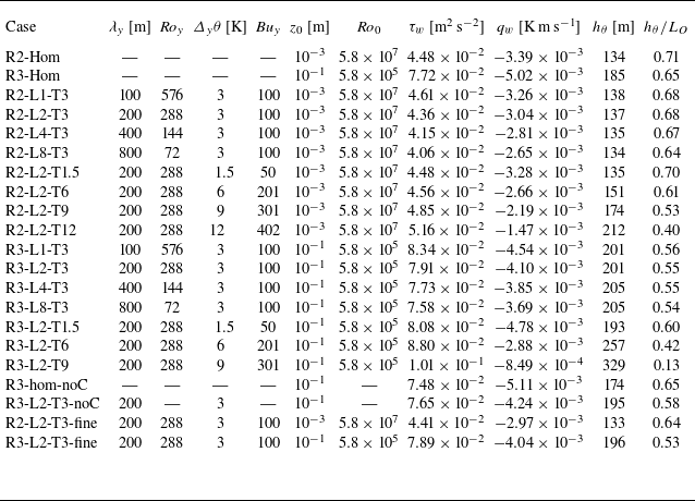
Overview of physical and simulation parameters that are common for all simulations in the present paper.

*
The domain length and width of cases with
 $\lambda _y=800$
m was adapted to 800 m, see text.
2.4. Description of case set-up and non-dimensionalisation
The LES cases of heterogeneous stably stratified boundary layers are derived from the homogeneous steady SBL simulations with subsidence of Bon et al. (Reference Bon, Cal and Meyers2024, cf. their table 1). The relevant physical and numerical parameters that all simulations have in common are summarised in table 1. Considering dimensional values, we use a fixed linear gradient of subsidence velocity,
 $\varGamma _w\equiv {\textrm{d}}w_s/{\textrm{d}}z=1.25\times 10^{-5}\,\textrm{s}^{-1}$
, and the difference between the prescribed mean surface temperature and the potential temperature of the free atmosphere
 $\varDelta _z\theta = \theta _\infty -\langle \theta _s\rangle$
equals 3 K (cf. figure 2). Note that both
 $\theta _\infty$
and
 $\theta _s$
remain constant in time, and therefore the vertical temperature difference
 $\varDelta _z\theta$
does not change either. Identical to the GABLS1 benchmark intercomparison case for SBL flows (Beare et al. Reference Beare2006), we set the reference temperature
 $\theta _r = 263.5$
K, acceleration due to gravity
 $g=9.81$
m s
 $^{-2}$
, geostrophic wind magnitude
 $G=8$
m s
 $^{-1}$
and Coriolis frequency
 $f_c = 1.39 \times 10^{-4}$
s
 $^{-1}$
. The latter parameter corresponds to a latitude of 73
 $^{\circ}$
N, which has been adopted in many other LES studies of the canonical SBL (e.g. Stoll & Porté-Agel Reference Stoll and Porté-Agel2009; Mironov & Sullivan Reference Mironov and Sullivan2016; Sullivan et al. Reference Sullivan, Weil, Patton, Jonker and Mironov2016). The domain size and grid resolution of the simulations here is also identical to that employed for the homogeneous SBLs of Bon et al. (Reference Bon, Cal and Meyers2024), as reported in table 1. The adequacy of this numerical domain for heterogeneous simulations is addressed in Appendix A through a succinct sensitivity analysis.
In the previous work by Bon et al. (Reference Bon, Cal and Meyers2024), the governing equations (2.1) of the steady-state homogeneous SBL subjected to linear subsidence were argued to be fully determined by a set of five input parameters, i.e.
 $G, f_c, z_0, \varDelta _z B, \varGamma _w$
. Here, we denote the vertical buoyancy difference
 $\varDelta _z B\equiv g/\theta _r (\theta _\infty - \langle \theta _s\rangle ) = g/\theta _r \varDelta _z\theta$
. Dimensional analysis then reveals that a set of three non-dimensional groups can be formed, consisting of a (vertical) buoyancy number
 $\textit{Bu}_z \equiv \varDelta _z B /(Gf_c)$
, surface Rossby number
 $\textit{Ro}_0 \equiv G/(f_c z_0)$
and subsidence number
 $\varPi _w \equiv \varGamma _w/f_c$
(cf. (9) of Bon et al. Reference Bon, Cal and Meyers2024). In all the present cases, the non-dimensional Buoyancy number
 $\mathit{\textit{Bu}_z} = 100$
and subsidence number
 $\varPi _w=0.09$
correspond to the ‘base configuration’ of Bon et al. (Reference Bon, Cal and Meyers2024). Note that the subscript
 $z$
is added here to the buoyancy number to emphasise that it concerns a vertical temperature difference and to distinguish it from the horizontal (surface) buoyancy number introduced later. Regarding the surface Rossby number
 $\textit {Ro}_0$
, denoting the scale separation between the Rossby radius
 $G/f_c$
and the surface roughness
 $z_0$
, we consider two different scenarios. One where
 $z_0 = 10^{-3}$
m (
 $\textit{Ro}_0 = 5.8\times 10^{7}$
), corresponding to the base configuration (case S3B2R2 of Bon et al. Reference Bon, Cal and Meyers2024, abbreviated to ‘R2’ here) and a second scenario where
 $z_0 = 10^{-1}$
m (
 $\textit{Ro}_0 = 5.8\times 10^{5}$
). The latter conforms to the GABLS1 case (Beare et al. Reference Beare2006) and case R3 of Bon & Meyers (Reference Bon and Meyers2024), representing typical onshore roughness. We remind the reader that equal roughness lengths are assumed for momentum and heat, i.e.
 $z_{0h} = z_{0m} = z_0$
for simplicity.
The inclusion of surface heterogeneity gives rise to a huge parameter space, as the heterogeneity, distribution and geometry can be varied in many ways (as previously pointed out by e.g. Kostelecky & Ansorge Reference Kostelecky and Ansorge2025). Similar to the heterogeneous channel flows considered by Bon & Meyers (Reference Bon and Meyers2022), we limit ourselves here to strips of high and low temperature that are oriented parallel to the surface wind, as illustrated in figure 2. We note that the sharp transitions in the boundary conditions were smoothed over a few grid points using a narrow Gaussian filter in the way described by Bon et al. (Reference Bon, Broos, Cal and Meyers2023, Appendix A.1) to avoid spurious oscillations in our spectral code. Considering figure 2, it is clear that the surface heterogeneity configuration is fully defined by two parameters: the surface temperature contrast
 $\varDelta _y\theta$
between the warm and cold strips, and the wavelength
 $\lambda _y$
which corresponds to two times the strip width. Regarding the dimensional analysis described previously, two new dimensionless groups are introduced by the surface heterogeneity. Using again the Rossby radius
 $G/f_c$
and inverse Coriolis frequency
 $1/f_c$
as the length and time scale to non-dimensionalise the problem, we define
 \begin{equation} \mathit{\textit{Ro}_y} = \frac {G}{f_c \lambda _y} \quad \textrm{and} \quad \mathit{\textit{Bu}_y} = \frac {g}{\theta _r} \frac {\varDelta _y\theta }{Gf_c}. \end{equation}
We can interpret the first as a (spanwise) heterogeneity Rossby number, representing the ratio between inertial forces at the heterogeneity scale (
 $\sim\!G^2/\lambda _y$
) and Coriolis acceleration (
 $\sim\!f_cG$
). The spanwise buoyancy number
 $\textit{Bu}_y$
is the ratio of acceleration due to surface buoyancy differences and Coriolis forcing. In § 3.3, these parameters are related to previously proposed dimensionless groups that describe surface heterogeneity (i.e. the heterogeneity Richardson number
 $\textit{Ri}_h$
from Fogarty & Bou-Zeid Reference Fogarty and Bou-Zeid2023 and heterogeneity parameter
 $\mathcal{H} = \textit{Bu}_{y}/\textit{Ro}_{y}$
introduced by Margairaz et al. Reference Margairaz, Pardyjak and Calaf2020b
).
All simulations that have been performed in the present study are outlined in table 2. There are two main sets of simulations that are used to systematically examine the effect of changing the surface temperature difference and wavelength separately. Two subsets of simulations with the surface temperature contrast fixed to 3 K and
 $\lambda _y \in \{100, 200, 400, 800\}$
m were conducted, for
 $z_0 = 10^{-3}$
m and
 $z_0 = 10^{-1}$
m. These cases are labelled R2-L
 $\{\lambda _y/100\}$
-T3 and R3-L
 $\{\lambda _y/100\}$
-T3, respectively. Since the SBL depth for the homogeneous R2 and R3 cases was approximately 130–200 m (Bon et al. Reference Bon, Cal and Meyers2024), these characteristic heterogeneity length scales are indeed of the same order as the boundary-layer height and are therefore expected to generate large-scale secondary flows. We note that the two cases with
 $\lambda _y=800$
m required a larger horizontal domain size; therefore, both the width and length of the domain were doubled to 800 m, while keeping the grid resolution equal to the other cases (i.e.
 $N_x$
and
 $N_y$
were also increased by a factor 2). In addition to varying
 $\lambda _y$
, two more subsets of cases where the surface heterogeneity strip width is fixed to 200 m, but with
 $\varDelta _y\theta \in \{1.5, 3, 6, 9, 12\}$
K are considered. We refer to these cases as R2(3)-L2-T
 $\{\varDelta _y\theta \}$
, where it is remarked that there is no ‘R3’-case with
 $\varDelta _y\theta =12$
K for reasons that will be explained in § 3.2. It is relevant to note here that the range of surface temperature differences and heterogeneity length scales is in line with earlier LES studies into thermal surface heterogeneity (Stoll & Porté-Agel Reference Stoll and Porté-Agel2009; Mironov & Sullivan Reference Mironov and Sullivan2016; Margairaz et al. Reference Margairaz, Pardyjak and Calaf2020a
; Fogarty & Bou-Zeid Reference Fogarty and Bou-Zeid2023).
Overview of simulations and bulk quantities. The heterogeneous surface temperature is defined by the characteristic wavelength
 $\lambda _y$
and surface temperature contrast
 $\varDelta _y\theta$
, or the corresponding dimensionless Rossby and buoyancy number
 $\textit{Ro}_y, \textit{Bu}_y$
. Simulations are further distinguished by the surface roughness
 $z_0$
or surface Rossby number
 $\textit{Ro}_0$
. Reported internal flow parameters are the horizontally averaged surface shear stress
 $\tau _w$
, heat flux
 $q_0$
thermal boundary-layer depth
 $h_\theta$
and stability indicator
 $h_\theta /L_O$
, where
 $L_O = -\theta _r\tau _w^{3/2}/(\kappa g q_0)$
.

Each of these cases was initialised from the latest instantaneous flow field of the corresponding homogeneous simulation (R2-hom or R3-hom in table 2). (Since the simulations with
 $\lambda _y=800$
m employed a larger computational domain, we used a tiling-approach to periodically extend the initial field in the
 $x$
- and
 $y$
-directions (similar to Gomez et al. Reference Gomez, Lundquist, Mirocha and Arthur2023; Lanzilao & Meyers Reference Lanzilao and Meyers2024). To break the periodicity and fill the Fourier modes that are zero after the periodic expansion, the tiled field was slightly perturbed at one horizontal location. Otherwise, the streamwise velocity field remained periodic between the patches as a result of the meticulous spectral discretisation.) The heterogeneous surface boundary conditions (§ 2.1), wind-angle controller and geostrophic damping (§ 2.3) were applied from the beginning of the simulation. The flow was then advanced for 12–24 physical hours (
 $\textit{tf}_c \approx 6{-}12$
), allowing the simulation to reach a steady state. Since the thermal surface heterogeneity can be expected to alter the mean surface heat flux and/or boundary layer height, this startup phase is required to guarantee that a new thermal equilibrium as described by Bon et al. (Reference Bon, Cal and Meyers2024) is established. Moreover, during this period, the geostrophic wind direction is turned by the wind-angle controller (cf. § 2.3) to obtain surface flow aligned with the surface temperature transitions. Subsequently, all simulations were run for a period of 12 dimensional hours (
 $T_{av}f_c=6$
) which was used to collect mean flow statistics. In agreement with the simulations reported by Bon et al. (Reference Bon, Cal and Meyers2024), this duration roughly conforms with a full inertial period. The wind-angle controller and geostrophic damping could in principle be turned off when the flow has reached a steady state. Although we did not do that in the present simulations, test simulations of the steady data collection period with and without the controller revealed no significant impact on simulation results of interest.
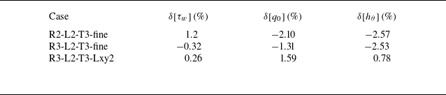
The cases reported in the lower rows of table 2 are included for comparison of several different simulation features, as will be further detailed throughout this text. In particular, the two simulations with suffix ‘-fine’ were performed with a doubled grid resolution in all directions to investigate how the representation of thermal surface heterogeneity is influenced by changes in grid resolution. These cases are further discussed in Appendix A. In the two simulations labelled with -noC, the Coriolis force and geostrophic forcing were replaced by a streamwise pressure forcing as explained in more detail Appendix B.
3. Results
We first systematically investigate the influence of altering the strip width
 $\lambda _y$
in § 3.1, followed by considering different surface temperature contrasts
 $\varDelta _y\theta$
in § 3.2. New approaches to scale mean flow characteristics are proposed in § 3.3, while we examine the local variations of surface fluxes in § 3.4.
3.1. Impact of strip width
In this section, we discuss the simulations where the heterogeneity wavelength
 $\lambda _y$
is varied between 100 and 800 m. Time- and horizontally averaged profiles of all cases with equal surface temperature difference but differing strip widths are presented in figure 4. To enable mutual comparison, all values in figure 4 are normalised by a reference thermal boundary layer height
 $h_{rh}$
and surface fluxes from case R3-hom. Here, the thermal boundary-layer height
 $h_\theta$
is defined as the level at which
 $(\langle \theta \rangle -\theta _s)/\varDelta _z\theta = 99\,\%$
. This criterion has been shown by Bon et al. (Reference Bon, Cal and Meyers2024) to provide a consistent characterisation of the SBL depth in thermal equilibrium. With this definition, the ratio between the strip width and SBL depth,
 $\lambda _y/h_\theta$
, ranges from approximately 0.7 to roughly 6 (cf. table 2 and figure 10
b), which is in line with previous studies into surface-induced secondary motions in channel flows (e.g. Chung, Monty & Hutchins Reference Chung, Monty and Hutchins2018; Bon & Meyers Reference Bon and Meyers2022; Salesky et al. Reference Salesky, Calaf and Anderson2022; Schäfer et al. Reference Schäfer, Frohnapfel and Mellado2022). In figure 4 and subsequent figures, red lines indicate cases from set R2 with
 $z_0=10^{-3}$
m, while blue lines indicate cases from set R3 (with
 $z_0=10^{-1}$
m). Overall, the difference between the red and blue lines evidently shows that larger surface roughness length leads to a deeper SBL, with larger surface fluxes and a higher low-level jet.
Mean profiles of (a) wind speed normalised by geostrophic value, (b) flow angle with respect to surface wind, (c) potential temperature deviation relative to vertical temperature difference, (d) normalised total vertical shear stress and (e) normalised total vertical heat flux for cases with varying heterogeneity wavelength
 $\lambda _y$
. Darker lines indicate larger
 $\lambda _y$
, while blue and red colours refer to simulations with
 $z_0=10^{-1}$
m and
 $z_0=10^{-3}$
m, respectively. Profiles are normalised by the thermal boundary layer height and surface fluxes from case R3-hom.

Comparing the heterogeneous cases to the homogeneous ones (black, grey lines), we observe that the the boundary-layer height is slightly increased, the surface momentum flux is nearly equal while the surface heat flux is reduced compared with the corresponding uniform-temperature cases. The profiles of the heterogeneous cases also show stronger velocity and potential temperature gradients in the near-surface region, while the potential temperature in the bulk of the SBL is significantly increased. For both Rossby numbers (red and blue lines), the influence of thermal surface heterogeneity on the mean profiles is qualitatively similar.
With growing strip widths (darker lines), the impact of thermal surface heterogeneity increases: the near-surface velocity and temperature gradients increase, boundary-layer depth grows slightly more and the magnitude of the surface heat flux throughout the boundary layer is further diminished. This is opposed to the findings from Stoll & Porté-Agel (Reference Stoll and Porté-Agel2009), who investigated an SBL with streamwise heterogeneous surface temperature with
 $\varDelta _x\theta =3$
and 6 K, and
 $\lambda _x=200$
, 400 and 800 m, and concluded that the potential temperature profiles did not significantly depend on the horizontal heterogeneity length scale. Hence, mean flow orientation is a crucial parameter when considering surface heterogeneity effects (Anderson Reference Anderson2020; Mironov & Sullivan Reference Mironov and Sullivan2025).
To quantify the mean flow heterogeneity, we employ the triple decomposition framework that has been widely used in studies into secondary flows (e.g. Raupach & Shaw Reference Raupach and Shaw1982; Vanderwel et al. Reference Vanderwel, Stroh, Kriegseis, Frohnapfel and Ganapathisubramani2019; Wangsawijaya et al. Reference Wangsawijaya, Baidya, Chung, Marusic and Hutchins2020; Calaf et al. Reference Calaf, Vercauteren, Katul, Giometto, Morrison, Margairaz, Boyko and Pardyjak2022; Schäfer et al. Reference Schäfer, Frohnapfel and Mellado2022). As illustrated in figure 5, turbulent flow variables are split into a horizontal-time average
 $\langle \overline {u}\rangle$
(where the overline denotes a time average), a turbulent (or ‘random’) fluctuation denoted by
 $u' = a-\overline {a}$
and a dispersive (or ‘coherent’) fluctuation indicated by
 $\overline {u}'' \equiv \overline {u} - \langle \overline {u}\rangle$
. Hence, the latter represents the horizontal heterogeneity of the mean flow, which is inherently zero in a homogeneous boundary layer. When this space–time averaging procedure is applied to transport equations of momentum or heat, new covariance terms (i.e. ‘dispersive fluxes’) naturally emerge (e.g. Raupach & Shaw Reference Raupach and Shaw1982; Vanderwel et al. Reference Vanderwel, Stroh, Kriegseis, Frohnapfel and Ganapathisubramani2019; Forooghi et al. Reference Forooghi, Yang and Abkar2020; Margairaz et al. Reference Margairaz, Pardyjak and Calaf2020a
; Calaf et al. Reference Calaf, Vercauteren, Katul, Giometto, Morrison, Margairaz, Boyko and Pardyjak2022).
Illustrative example of triple decomposition of streamwise velocity field in case R3-L2-T3. Red and blue patches indicate high and low surface temperature, respectively. The top row illustrates the classic Reynolds decomposition
 $u = \overline {u} + u'$
, whereas the bottom row reveals the decomposition of
 $\overline {u}$
into a horizontal mean
 $\langle \overline {u}\rangle$
and dispersive part
 $\overline {u}''$
. Figure inspired by Wangsawijaya et al. (Reference Wangsawijaya, Baidya, Chung, Marusic and Hutchins2020, figure 3).

Cross-stream planes of streamwise velocity deviation
 $\langle \overline {u}-\langle \overline {u}\rangle _{xy}\rangle _x$
, averaged over time and the streamwise direction. (a–d) Cases R3-L1-T3, R3-L2-T3, R3-L4-T3, R3-L8-T3. Vectors are obtained from the dispersive in-plane velocity components
 $\overline {v}'', \overline {w}''$
, while red and blue patches at the bottom correspond to high and low surface temperature. The red contour traces the line where the vertical temperature gradient is 0.

To obtain a general overview of the mean flow, figure 6 provides
 $x$
-averaged slices of the time-averaged dispersive velocity fields in the cases with
 $z_0=10^{-1}$
m with varying
 $\lambda _y$
. The streamwise velocity deficit
 $\langle \overline {u}''\rangle _x = \langle \overline {u} - \langle \overline {u}\rangle _{xy}\rangle _x$
reaches 20 % of the geostrophic wind
 $G$
. From both figures 5 and 6, it is clear that high-momentum pathways (HMPs,
 $\langle \overline {u}''\rangle _x\gt 0$
) are formed above the low-temperature patches, and low-momentum pathways (LMPs,
 $\langle \overline {u}''\rangle _x\lt 0$
) above the regions with higher temperature. It should be emphasised that the in-plane vectors here also represent the dispersive velocities, i.e. the mean
 $\langle \overline {v}\rangle _{\textit{xy}}$
and
 $\langle \overline {w}\rangle _{xy}(=0)$
are subtracted from the respective velocity components. Note that the mean flow (that was subtracted) is along the
 $x$
-direction at the ground surface and turns towards the geostrophic wind direction (away from the pressure gradient) when moving upward (i.e. to the left on figure 6). Figure 6 demonstrates that secondary circulations are induced in thermally heterogeneous stable Ekman layers and their extent increases as
 $\lambda _y$
increases. However, in contrast to secondary motions in unidirectional channel flows (Bon & Meyers Reference Bon and Meyers2022; Salesky et al. Reference Salesky, Calaf and Anderson2022), the flow is highly asymmetric as the HMPs and LMPs are tilted towards the direction of the mean spanwise velocity. Despite this difference, Appendix B demonstrates that the impact of spanwise surface temperature heterogeneity on mean flow profiles in SBLs with secondary circulations that are asymmetric due to Coriolis effects remains broadly similar to that in analogous cases without Coriolis forcing.
Further, we note that the bold red curves near the surface in figure 6 trace the height where
 $\partial \langle \overline {\theta }\rangle _x/\partial z = 0$
. As the mean temperature gradient in the SBL is positive, the areas below these lines exhibit a negative temperature gradient and therefore unstable stratification. These convective regions are obviously centred above the strips with relatively high surface temperature, while both the vertical an horizontal extent increases as the heterogeneity length scale
 $\lambda _y$
increases.
(a, b) Decomposition of (a) vertical momentum and (b) heat flux into dispersive (full lines) and turbulent (dashed lines) parts for cases with
 $\lambda _y=100$
and 800 m and the homogeneous reference cases. Line colours are similar to figure 4. All cases are normalised by their respective surface heat (
 $q_0$
) and momentum fluxes (
 $\tau _w$
) and thermal boundary layer height
 $h_\theta$
. (c, d) Square root of normal stresses of (c) streamwise velocity and (d) potential temperature variance, decomposed in dispersive and turbulent parts.

To evaluate the contribution of the dispersive motions to the vertical mixing of momentum and heat, figure 7(a, b) presents a decomposition into dispersive and turbulent fluxes of momentum and heat. Compared with the triple decomposition in some DNS and experimental studies (e.g. Medjnoun, Vanderwel & Ganapathisubramani Reference Medjnoun, Vanderwel and Ganapathisubramani2020; Stroh et al. Reference Stroh, Schäfer, Forooghi and Frohnapfel2020; Bon & Meyers Reference Bon and Meyers2022; Bon et al. Reference Bon, Broos, Cal and Meyers2023), the viscous transport is ignored, while the turbulent transport is computed as the sum of the SGS and resolved fluxes. We refer to Appendix A for an evaluation of their individual contributions. For clarity of presentation, only the homogeneous cases and the cases with the minimum and maximum strip widths are displayed. Panel (a) reveals that the relative contribution of dispersive transport to the total vertical mixing of momentum is at most approximately 20 %, although the (relative) height where the maximum occurs rises for larger
 $\lambda _y$
and smaller surface roughness. The relative magnitude of the dispersive heat flux appears to decrease with
 $\lambda _y$
for the R3 (blue) cases, whereas it remains more or less constant for the R2 (red) cases. The increment in the level of the peak in dispersive fluxes can be related to the growing size of the secondary flows for larger surface heterogeneity. We point out that the fact that the dispersive heat flux is opposite to the turbulent one, as well as the reduction of the total surface heat flux due to spanwise temperature heterogeneity (cf. figure 4
e), are consistent with the findings in the DNS of stably stratified channel flows presented by Bon & Meyers (Reference Bon and Meyers2022), Bon et al. (Reference Bon, Broos, Cal and Meyers2023) and Mironov & Sullivan (Reference Mironov and Sullivan2025).
Figures 7(c) and 7(d) present the spatial standard deviation of mean streamwise velocity (
 $\langle \overline {u}''\overline {u}''\rangle ^{1/2}$
) and temperature (
 $\langle \overline {\theta }''\overline {\theta }''\rangle ^{1/2}$
). The round markers in panel(c) indicate the ‘blending height’
 $z_b$
, which is often loosely defined as the elevation above which the flow becomes approximately horizontally homogeneous, i.e. where turbulent mixing or advection has blended the signature of individual surface patches (Wieringa Reference Wieringa1976; Mahrt Reference Mahrt2000). Here, we define it as the level where
 $\langle \overline {u}''\overline {u}''\rangle ^{1/2}$
approaches zero, as further explained in § 3.3. Figure 7(c) shows that the blending height, or the ‘penetration depth’ of the surface heterogeneity, increases from
 $z_b/h_\theta \approx 0.4$
for
 $\lambda _y$
= 100 m (‘L1’-cases) to near the boundary-layer height for cases with
 $\lambda _y =$
800 m Particularly, the latter cases exhibit a second peak in dispersive stresses around
 $h_\theta$
. Examination of the streamwise-averaged dispersive flow field in figure 6(d) reveals that tertiary vortices are formed near the top of the boundary layer, above the wall-attached secondary vortices. This vortex ‘stacking’ in spanwise heterogeneous SBLs has been previously observed by Forooghi et al. (Reference Forooghi, Yang and Abkar2020) and Bon & Meyers (Reference Bon and Meyers2022).
An explanation for the seemingly deeper impact of surface heterogeneity with
 $\lambda _y=800$
m at lower surface roughness may simply lie in the different SBL depth. This suggests that the effect of secondary flows induced by spanwise surface heterogeneity depends on the ratio
 $\lambda _y/h_\theta$
, which is larger in the R2 cases, consistent with previous findings in the context of both roughness-induced (e.g. Chung et al. Reference Chung, Monty and Hutchins2018; Medjnoun, Vanderwel & Ganapathisubramani Reference Medjnoun, Vanderwel and Ganapathisubramani2018; Wangsawijaya et al. Reference Wangsawijaya, Baidya, Chung, Marusic and Hutchins2020) and thermally induced secondary flows (Bon & Meyers Reference Bon and Meyers2022). We examine this idea further in § 3.3. We note that in the DNS of spanwise heterogeneous channel flows presented by e.g. Chung et al. (Reference Chung, Monty and Hutchins2018) and Bon & Meyers (Reference Bon and Meyers2022), the impact of surface heterogeneity was maximised for intermediate surface wavelengths (
 $\lambda _y/h_c \approx 1$
, see e.g. figure 3 of Bon & Meyers Reference Bon and Meyers2022), whereas here we find that the impact on the SBL keeps growing as the strip width increases up to
 $\lambda _y/h_\theta \approx 6$
(cf. figure 10). This contrast can be ascribed to the fact that the upper wall in these channel flows was also heterogeneous, generating opposing circulations extending downward towards the channel centre. As a result, these channel flows were symmetric about their centre plane and the vertical size of the secondary motions is limited by the fixed half-channel height. In contrast, the SBL depth in the atmosphere is not fixed but a dynamical result of the balance between boundary-layer turbulence and stratification. Buoyancy-induced secondary circulations modify both, as illustrated in figures 4 and 7, thereby increasing the boundary-layer depth and hence lifting the vertical confinement for the secondary flows.
Regarding the turbulent fluctuations, figure 7(c) reveals that they are remarkably similar in all cases and do not deviate much from the homogeneous cases. Hence, total fluctuation energy (of the turbulent and dispersive fluctuations combined, not shown) is increased by the thermal surface heterogeneity. Particularly, we note that the spatial variance of the streamwise velocity is of the same magnitude as the temporal variance near the surface, This is in line with the observations in the stable channel flows with heterogeneous wall temperature at finite Reynolds number studied by Bon et al. (Reference Bon, Broos, Cal and Meyers2023).
Considering the dispersive temperature variance, figure 7(d) shows that it decreases from its maximum at the surface to zero around
 $z/h_ \theta = 0.2$
, indicating that the blending height for temperature is significantly lower than for momentum (in line with the DNS of Bon & Meyers Reference Bon and Meyers2022; Bon et al. Reference Bon, Broos, Cal and Meyers2023). Moreover, we emphasise that the surface value of
 $\langle \overline {\theta }''\overline {\theta }''\rangle ^{1/2}$
is directly imposed by the heterogeneous temperature boundary conditions. Considering that the surface temperature is a (smoothed) square wave with peak-to-peak amplitude
 $\varDelta _y\theta$
, the spatial standard deviation of the surface temperature is approximately
 $\varDelta _y\theta /2$
and should not depend on the wavelength. Nevertheless, the values of
 $(\overline {\theta }''\overline {\theta }'')^{1/2}$
at the first grid point are notoriously different, indicating local differences in heat transfer between the surface and the first grid point, which appears to be not only affected by the thermal roughness length (
 $\textit{Ro}_0$
, compare blue and red lines), but also by the surface wavelength. The local surface fluxes are further inspected in § 3.4. Lastly, we observe that the turbulent temperature fluctuations (dashed lines) have their maximum within the strongly stratified inversion layer for all cases, which can be related to internal gravity waves (Nappo Reference Nappo2012; Lloyd, Dorrell & Caulfield Reference Lloyd, Dorrell and Caulfield2022). Note that this peak in temperature variance also occurs in the entertainment zone of convective boundary layers (e.g. Sullivan & Patton Reference Sullivan and Patton2011).
Mean profiles of (a) wind speed normalised by geostrophic value, (b) flow angle with respect to surface wind, (c) potential temperature deviation relative to vertical temperature difference, (d) normalised total vertical shear stress and (e) normalised total vertical heat flux for cases with varying surface temperature contrast. Darker lines indicate larger
 $\varDelta _y\theta$
, while blue and red colours refer to simulations with
 $z_0=10^{-1}$
m and
 $z_0=10^{-3}$
m, respectively. Profiles are normalised by the thermal boundary layer height and surface fluxes from case R3-hom.

(a, b) Decomposition of (a) vertical momentum and (b) heat flux into dispersive (full lines) and turbulent (dashed lines) parts for cases with
 $\varDelta _y\theta =1.5$
and
 $9$
K and the homogeneous reference cases. Line colours are similar to figure 8. All cases are normalised by their respective surface heat (
 $q_0$
) and momentum fluxes (
 $\tau _w$
) and thermal boundary layer height
 $h_\theta$
. (c, d) Square root of normal stresses of (c) streamwise velocity and (d) potential temperature variance, decomposed in dispersive and turbulent parts.

3.2. Impact of surface temperature difference
Mean profiles of all cases with
 $\lambda _y = 200$
m and changing surface temperature difference are presented in figures 8 and 9. Generally, increasing
 $\varDelta _y\theta$
leads to an elevated low-level jet, a stronger near-surface mean velocity gradient and less wind turning over the full boundary layer (figures 8
a and 8
b). Moreover, the potential temperature in an SBL over a heterogeneous surface with larger temperature contrasts is higher and better vertically mixed, while the magnitude of the total heat flux is reduced. In contrast to the cases with changing patch width in the previous section, we observe that the surface temperature substantially influences the total momentum flux throughout the boundary layer. These results are roughly consistent with previous findings of Stoll & Porté-Agel (Reference Stoll and Porté-Agel2009) and Mironov & Sullivan (Reference Mironov and Sullivan2016) in LES of quasi-steady heterogeneous SBLs with streamwise thermal surface heterogeneity.
In case R3-L2-T9, the bulk temperature is so much increased and the heat flux magnitude so far reduced that the boundary layer is almost neutrally stratified, and, consequently, reaches the top of the computational domain. Therefore, the results of this simulation should be interpreted with caution. Given the extreme nature of this case, we did not perform an R3 simulation with
 $\varDelta _y\theta = 12$
K, as this would require a substantially higher domain where assuming a uniform background temperature above the SBL becomes less realistic. In the cases with smaller
 $z_0$
(R2, red lines), both the mean and local surface heat fluxes are smaller due to less efficient surface–atmosphere exchange (see also the next to sections), and therefore, the absolute impact on the SBL is not as large as for the R3 (blue) cases with identical
 $\varDelta _y\theta$
.
The dispersive fluxes and normal stresses of cases with
 $\varDelta _y\theta =1.5$
and 9 K are presented in figure 9. The penetration depth of the flow heterogeneity (scaled with SBL depth
 $h_\theta$
), i.e. the height above which the dispersive stresses vanish as indicated by the square markers in panel (c), is more or less similar in all cases. Meanwhile, the relative contribution of the dispersive fluxes to the total vertical mixing substantially increases for larger surface temperature differences (panels a and b). These results are roughly opposite to the findings for changing
 $\lambda _y$
in the previous section, where the blending height was significantly changed by varying
 $\lambda _y$
while the magnitude of the dispersive stresses was less responsive. Here, the dispersive momentum flux attains up to 50 % of the surface shear stress for large
 $\varDelta _y\theta$
, while the magnitude of the dispersive heat flux is more than 10 times larger than the mean surface heat flux
 $q_0$
. Figure 9(d) shows significant variations in temperature variance near the surface, which is not only imposed by the different values of
 $\varDelta _y\theta$
, but also a result of the differences in
 $z_0$
as described in the previous section (compare the blue and red lines with equal
 $\varDelta _y\theta$
). As pointed out in the works of Mironov & Sullivan (Reference Mironov and Sullivan2016, Reference Mironov and Sullivan2023, Reference Mironov and Sullivan2025), temperature variance occurs as the buoyancy production term in the budget equation for vertical heat flux and, therefore, is a source of positive (upward) heat flux. This argument explains the substantial increase in the (upward) dispersive heat flux for larger
 $\varDelta _y\theta$
in figure 9(b).
3.3. Scaling of mean flow properties
The preceding two sections have demonstrated that the spanwise heterogeneity length scale and surface temperature contrast modify the SBL in different ways. Here, we investigate quantitative relations between the surface heterogeneity and mean flow properties.
The first quantity of interest that we will consider is the blending height
 $z_b$
, or the level up to which the heterogeneity effects penetrate into the boundary layer (Wieringa Reference Wieringa1976). Although a consistent formal definition of the blending height is lacking in the literature (e.g. Mahrt Reference Mahrt2000), it is often based on the level at which the streamwise velocity becomes homogeneous (Bou-Zeid et al. Reference Bou-Zeid, Meneveau and Parlange2004; Miller & Stoll Reference Miller and Stoll2013; Calaf, Higgins & Parlange Reference Calaf, Higgins and Parlange2014). This height is of particular relevance for large-scale modelling, where mean similarity profiles can only be applied above the blending height (e.g. Stoll & Porté-Agel Reference Stoll and Porté-Agel2009; Bou-Zeid et al. Reference Bou-Zeid, Anderson, Katul and Mahrt2020), and practical applications such as wind energy (e.g. Porté-Agel et al. Reference Porté-Agel, Bastankhah and Shamsoddin2020; Bon et al. Reference Bon, Van Craenenbroeck and Meyers2025). In the present work, we define
 $z_b$
as the height where the square root of the dispersive streamwise velocity variance
 $\langle \overline {u}''\overline {u}''\rangle _{xy}^{1/2}$
drops below 0.1 % of the geostrophic wind magnitude
 $G$
. This level is indicated by the circular markers in figure 7(c) and the square markers in figure 9(c), and appears to accurately trace the height where the dispersive variance vanishes. We point out that definitions based on e.g. dispersive vertical velocity or potential temperature are more ambiguous in the present cases, as they do not approach zero in a consistent manner (not shown).
Blending height
 $z_b$
for all R2 (
 $z_0=10^{-3}$
m, red) and R3 (
 $z_0=10^{-1}$
m, blue) simulations with varying surface temperature difference (square markers) and changing heterogeneity length scale (round markers). Colours are identical to the figures in the previous section, with darker colour indicating a higher value of
 $\varDelta _y\theta$
or
 $\lambda _y$
. Panel (a) shows
 $z_b$
as function of
 $\lambda _y$
, whereas in panel (b), both are scaled with the SBL depth
 $h_\theta$
of each simulation. The grey dashed line in panel (b) represents
 $0.4(\lambda _y/h_\theta )^{1/2}$
.

In figure 10(a), we plot
 $z_b$
as a function of
 $\lambda _y$
for all heterogeneous R2 and R3 cases. Square and round markers indicate simulations with varying
 $\varDelta _y\theta$
and
 $\lambda _y$
, respectively, whereas darker colours denote higher values. It is evident that in the absolute sense, a stronger surface temperature contrast, larger strip width and larger surface roughness lead to deeper penetration above the surface. In panel (b), both
 $z_b$
and
 $\lambda _y$
are non-dimensionalised with the thermal boundary layer depth
 $h_\theta$
of each respective simulation. As noted in the previous section, the effect of varying
 $\varDelta _y\theta$
on the blending height is captured by the scaling with
 $h_\theta$
. That is, a larger surface temperature contrast leads to stronger secondary flows that penetrate deeper into the boundary layer, but the SBL depth is simultaneously increased (cf. figure 8) and therefore the effect on
 $z_b/h_\theta$
is mitigated. In fact, the relative penetration depth of the heterogeneity slightly decreases for larger
 $\varDelta _y\theta$
, indicated by the notion that the darker coloured square markers lie slightly below the lighter ones in figure 10(b). The SBL depth is not as much modified in the cases with changing heterogeneity length scale (cf. figure 4); therefore, the trends in figures 10(a) and 10(b) are similar. However, the blending heights of cases with different surface roughness (denoted by red and blue coloured markers) more or less collapse on one line when scaling with the SBL depth. The grey dashed line in figure 10(b) suggests that
 $z_b/h_\theta \sim (\lambda _y/h_\theta )^{1/2}$
, or equivalently
 $z_b \sim (\lambda _y h_\theta )^{1/2}$
, in the present simulations. From a physical point of view, it may be surprising that there is no global stability parameter included in this dependency. However, we point out that stratification effects are included implicitly through the boundary-layer depth. Particularly, a more stably stratified boundary layer will be shallower, resulting in a lower blending height. This should however be tested further for more strongly stratified boundary layers.
Scaling of (a, b) mean surface heat flux, (c) shear stress and (d) SBL depth of simulations with changing spanwise surface temperature heterogeneity and surface roughness, normalised by values from the corresponding homogeneous case. The horizontal axes of panels (a) and (b–d) respectively represent the heterogeneity parameter and a modified heterogeneity Richardson number, defined in (3.1). Squares (circles) symbolise simulation sets with with varying surface temperature contrast (heterogeneity length scale), while blue and red indicate simulations with higher (R3) and lower (R2) surface roughness.

Next, we examine the modification of surface heat and momentum flux that is caused by the spanwise surface heterogeneity, analogous to our previous DNS studies reported by Bon & Meyers (Reference Bon and Meyers2022) and Bon et al. (Reference Bon, Broos, Cal and Meyers2023). Two recently proposed dimensionless numbers to characterise the impact of thermal surface heterogeneity on the mean flow are the ‘heterogeneity parameter’
 $\mathcal{H}$
(Margairaz et al. Reference Margairaz, Pardyjak and Calaf2020b
) and the heterogeneity Richardson number
 $\textit{Ri}_h$
(Fogarty & Bou-Zeid Reference Fogarty and Bou-Zeid2023), respectively defined as
 \begin{equation} \mathcal{H} \equiv \frac {g}{\theta _r}\frac {\varDelta _y\theta{\kern-1pt} \lambda _y}{G^2} = \frac {\textit{Bu}_y}{\textit{Ro}_\lambda } \quad \textrm{and} \quad \textit{Ri}_h \equiv \frac {g}{\theta _r} \frac {\varDelta _y\theta h_\theta }{G^2} = \mathcal{H}\frac {h_\theta }{\lambda _y} = \frac {h_\theta\!f_c}{G}\textit{Bu}_y. \end{equation}
Both numbers represent a ratio of buoyancy acceleration generated by the heterogeneous surface (
 $g\varDelta _y\theta /\theta _r \equiv \varDelta _yB$
) to inertia generated by the mean wind (
 $G^2/h_\theta$
or
 $G^2/\lambda _y$
). The right-hand side in (3.1) illustrates that
 $\mathcal{H}$
is fully defined by external parameters in the present LES, whereas
 $\textit{Ri}_h$
depends on the SBL depth that is not known a priori.
Figure 11(a) shows the surface heat flux in the heterogeneous simulations normalised by the value of the corresponding homogeneous case (i.e. R2-hom or R3-hom), as a function of heterogeneity parameter
 $\mathcal{H}$
. Although the decrease of surface heat flux is generally stronger for larger
 $\mathcal{H}$
, the data clearly do not collapse. The simulation sets with different surface roughness (red and blue colours) show different dependencies on
 $\mathcal{H}$
. This is related to one of the caveats regarding the formulations of
 $\mathcal{H}$
highlighted by Margairaz et al. (Reference Margairaz, Pardyjak and Calaf2020b
): the buoyancy acceleration
 $g\varDelta _y \theta /\theta _r$
experienced by the near-surface air depends not only on the surface temperature contrast
 $g\varDelta _y T / T_r$
, but also on how effectively this temperature contrast is transferred to the overlying air. This is exemplified by the dispersive temperature variance in figure 7(d), demonstrating that the buoyancy difference between the different patches depends on both the horizontal heterogeneity length scale and the surface roughness. Considering figure 6, the strength of the horizontal dispersive fluxes likely plays a crucial role in the spanwise mixing of buoyancy, which is a compelling topic for future research. Furthermore, it should be noted that the efficiency of vertical heat transfer between the surface and first grid level is essentially parametrised by
 $z_{0h}$
in wall-modelled LES.
The simulation results of Margairaz et al. (Reference Margairaz, Pardyjak and Calaf2020b
), which all exhibited the same thermal roughness length (i.e.
 $z_{0h}=z_{0m}/10=10^{-2}$
m), scaled quite well as a function of
 $\mathcal{H}$
, and the present dataset reveals that any scaling parameter should somehow account for scenarios with different surface roughness. Moreover, Margairaz et al. (Reference Margairaz, Pardyjak and Calaf2020b
) propose that the impact of thermal dispersive fluxes is small for
 $\mathcal{H} \lt 1$
, intermediate for
 $1\lt \mathcal{H} \lt 5$
and ‘considerable’ for
 $\mathcal{H}\gt 5$
, for a broad range of unstably stratified conditions and thermal isotropic surface heterogeneity. Figure 11(a) (as well as the figures in the two preceding sections) provides evidence that stably stratified flows over spanwise surface temperature variations with
 $\mathcal{H}$
below 1 can already be substantially affected by thermal dispersive fluxes, indicating that the three proposed regimes are modified by the mean flow stratification and the shape of the surface temperature distribution.
Although the heterogeneity Richardson number
 $\textit{Ri}_h$
includes the boundary-layer depth, which can be regarded as a representation of (mean) flow stratification, it lacks a dependency on the surface heterogeneity wavelength. In an attempt to derive a new scaling parameter, we start from the definition of
 $\textit{Ri}_h$
as a ratio between two velocity scales (Fogarty & Bou-Zeid Reference Fogarty and Bou-Zeid2023):
 \begin{equation} \textit{Ri}_h = \frac {W_b^2}{G^2}, \end{equation}
where
 $W_b=(g/\theta _r \varDelta _y\theta h_\theta )^{1/2} = (\varDelta _y B h_\theta )^{1/2}$
is a buoyancy velocity scale. First, we propose replacing the SBL depth
 $h_\theta$
by the blending height
 $z_b$
, as this represents the height of the layer that is affected by the buoyancy acceleration. Based on figure 10(b) and the previous discussion, we parametrise
 $z_b$
as
 $(\lambda _y h_\theta )^{1/2}$
. Next, we consider
 $f_ch_\theta /G$
as a measure of the mean SBL stability, which can be interpreted as the ratio between the SBL depth and the height of a neutral Ekman layer that roughly scales as
 $G/f_c$
. All things considered, figure 11(b) demonstrates that the ratio
 $q_0/q_{0,hom}$
of all simulations in the current dataset collapses as a linear function of
 $\textit{Ri}_h f_c (\lambda _y h_\theta )^{1/2}/G$
or
 $\textit{Ri}_{h,b} f_ch_\theta /G$
with
 $\textit{Ri}_{h,b}$
a heterogeneity Richardson number based on the blending height.
Using the same scaling as in panel (b) for the impact of spanwise thermal surface heterogeneity on the surface shear stress and SBL depth, the cases with larger
 $\lambda _y$
were shifted too far to the right (not shown). Replacing the Rossby radius by
 $\lambda _y$
on the horizontal axis improved the collapse of data points as shown in figure 11(c, d). Since the physical mechanisms underlying these relations remain uncertain owing to the large number of interacting parameters, their universality should be further investigated over a broader range of conditions. Nevertheless, if such universal relations between surface fluxes over homogeneous and heterogeneous surfaces can be established, they would provide valuable guidance for the parametrisation of subgrid-scale heterogeneity in coarse-resolution models. It should be noted that the present correlations require the SBL depth, which is generally not known a priori. Therefore, they should be used in conjunction with existing estimation methods for determining the SBL depth (e.g. Zilitinkevich, Esau & Baklanov Reference Zilitinkevich, Esau and Baklanov2007; Bon et al. Reference Bon, Cal and Meyers2024; Narasimhan, Gayme & Meneveau Reference Narasimhan, Gayme and Meneveau2024; Shen et al. Reference Shen, Liu, Lu and Stevens2025).
3.4. Surface flux heterogeneity
Time- and streamwise-averaged distributions of (a) surface shear stress, (b) heat flux and (c) stability parameter (i.e. the ratio between SBL depth and Obukhov length) for simulation with spanwise heterogeneous surface temperature of varying strip width, normalised by results from the homogeneous case. Darker blue colours indicate cases with larger
 $\lambda _y$
. The spanwise coordinate is scaled with
 $\lambda _y$
and centred around a hot patch, indicated by the grey background. Dashed horizontal lines represent the mean of each simulation.

We conclude by examining the local surface fluxes rather than the horizontally averaged ones from the previous sections. Figure 12 displays the streamwise- and time-averaged surface shear stress
 $\langle \tau _w\rangle _x(y) = \langle (\overline {\tau }_{w1}^2(x,y) + \overline {\tau }_{w2}^2(x,y))^{1/2}\rangle _x$
(panel a) and heat flux
 $q_0(y) = -\langle \overline {u_*(x,y)\theta _*(x,y)}\rangle _x$
(panel b) for the R3 cases (
 $z_0=10^{-1}$
m) with varying wavelength as a function of spanwise distance
 $y$
. Note that
 $\tau _{w1}, \tau _{w2}$
and
 $q_0$
are imposed by the wall model described in § 2.2 and their time-averaged local values are given as output by SP-Wind. The curves are normalised by the horizontally averaged
 $\overline {u}_*^2$
and
 $|\overline {q_0}|$
from case R3-hom, while the spanwise coordinate is scaled by the surface heterogeneity length scale
 $\lambda _y$
and centred at a warm strip. The local heterogeneity parameter
 $h_\theta /\langle L_O\rangle _x$
is displayed in panel (c), where the streamwise and time-averaged Obukhov length was calculated as
 \begin{equation} \langle L_O\rangle _x(y) = -\biggl \lt \frac {\theta _r\overline {\tau }_w^{3/2}(x,y)}{\kappa g \overline {q}_0(x,y)}\biggr \gt _x. \end{equation}
Figure 12 shows that the surface momentum and heat fluxes are positive above the warm strip, while the stability parameter (hence,
 $L_O$
) is negative. These are all indications of locally unstable stratification, corresponding to the convective regions below the red curves in figure 6. The surface momentum flux is reduced above the colder strips, where the heat flux is negative and relatively constant over the patch. The observed asymmetry in surface shear stress is in line with the pronounced asymmetry of the secondary circulations in the presence of Coriolis effects (cf. figures 6 and 18). By contrast, the surface heat flux shows a nearly symmetric pattern, where the maxima occur around the edge of the patches. This is likely a result of local advection of relatively cold air from the colder patches over the warmer patch due to the secondary circulations (cf. figures 6 and 18), resulting in a sharp vertical temperature contrast and therefore large positive surface flux near the edge. We note that a similar observation has been reported by Stoll & Porté-Agel (Reference Stoll and Porté-Agel2009, their figure 2), where the mean flow was perpendicular to the temperature strips and the positive surface heat flux over the warm patch peaked at the upstream cold-to-hot transition. The spanwise development of the stability in figure 12(c) is similar to that of the surface heat flux. This is related to the fact that the horizontal variation in
 $\tau _w$
is significantly smaller than the modification of
 $q_0$
. The latter not only changes sign from the hot to the cold patch, but the local heat fluxes are also approximately an order of magnitude larger than the mean heat flux. This is again in line with the LES results presented by Stoll & Porté-Agel (Reference Stoll and Porté-Agel2009).
Same as figure 12, but for simulations with different surface temperature contrast where darker blue lines represent larger
 $\varDelta _y\theta$
. The spanwise coordinate here is centred around the centre of the domain, and the entire width of the computational domain is shown. Grey shaded areas indicate warm strips.

The spanwise distributions of the surface fluxes for the R3 cases with varying surface temperature are presented in figure 13. The arrangements are qualitatively similar to those in figure 12, except that the amplitude of the deviations from the mean fluxes substantially increases for larger surface temperature contrasts. As a result, the local stability parameter
 $h_\theta /L_O$
exceeds 20. It is relevant to point out here that in all cases with
 $\varDelta _y\theta \lt 2\varDelta _z\theta = 6$
K, both the colder and warmer strips individually would lead to a stable boundary layer since they are colder than the neutral upper atmosphere. Nevertheless, due to the presence of the colder strips, the relatively warmer strips become locally unstably stratified. As mentioned previously, this is a result of spanwise advection of near-surface cold air from the cold to the warm strips, as shown for instance in figure 2(a) of Bon & Meyers (Reference Bon and Meyers2022).
Lastly, we note that the cases with smaller surface roughness (R2, not shown) have similar patterns but with smaller variations from the mean, due to the prescribed less efficient land-atmosphere interaction (smaller
 $z_{0h}$
).
In general, this section highlights that the mean surface fluxes in a heterogeneous SBL may not fully capture the underlying physical processes at play. Although the rise in mean Obukhov length and decrease in the mean stability parameter
 $h_\theta /L_O$
(see table 2) suggest that surface temperature heterogeneity reduces stability of the boundary layer, the local fluxes present a different perspective. As the local gradients and flow stability substantially deviate from the mean stratification, more extreme phenomena can occur. Particularly, the strongly negative surface heat fluxes and small Obukhov length at the cold patches are indicators of the very stable regime, where turbulence may become intermittent (e.g. Mahrt Reference Mahrt2014; Kostelecky & Ansorge Reference Kostelecky and Ansorge2025). This puts severe reliance of LES results on the subgrid model and surface flux parametrisation, which may even rise the question whether LES is appropriate for these kind of studies. Nevertheless, the resolution study in Appendix A reveals that the surface fluxes are reasonably robust, despite a reduction of subgrid transport with finer grid resolution.
4. Conclusions
In the present work, the simulation set-ups from two of our previous studies, i.e. the DNS of stable channel flows with spanwise varying surface temperatures by Bon & Meyers (Reference Bon and Meyers2022) and the LES of the steady-state SBL subjected to subsidence of Bon et al. (Reference Bon, Cal and Meyers2024), were merged to examine buoyancy-induced secondary motions in a steady, subsidence-prone, moderately stable Ekman layer in LES at ‘infinite’ Reynolds number. Hence, the research presented here extends previous investigations into unidirectional low-Reynolds-number flows with spanwise surface temperature heterogeneity towards the stable atmospheric boundary layer with Coriolis effects. The considered surface consisted of long strips with high and low temperature, where the imposed surface temperature contrast
 $\varDelta _y\theta$
was varied from 1.5 to 12 K, and the heterogeneity wavelength
 $\lambda _y$
from 100 to 800 m. The near-surface wind was ensured to be parallel to the isotherms using a wind-angle controller that redirects the geostrophic forcing to accommodate the desired surface wind direction.
The simulation results demonstrate that spanwise thermal surface heterogeneity induces asymmetric secondary circulations that have a substantial impact on the mean state of the SBL, despite the deformation of the secondary flows due to Coriolis effects. The most important influence on the mean flow are the horizontal redistribution of streamwise velocity (i.e. formation of HMPs and LMPs) and upward dispersive transport of heat. In stably stratified boundary layers, the latter implies that the magnitude of the negative mean surface heat flux is considerably reduced, while near-surface temperature gradients are increased. Generally, both an increase of surface temperature contrast and larger strip width resulted in reduced surface heat flux and increased near-surface gradients of velocity and temperature, consistent with previous DNS studies of channel flows at small Reynolds numbers (Bon & Meyers Reference Bon and Meyers2022; Bon et al. Reference Bon, Broos, Cal and Meyers2023; Mironov & Sullivan Reference Mironov and Sullivan2025). In contrast to the previously considered channel flows where the flow is confined to the fixed channel height, one of the effects of surface heterogeneity in the present cases was to elevate the boundary-layer depth and low-level jet. This impact was most pronounced in cases where the surface temperature contrast was increased, resulting in the particular notion that the penetration depth of the secondary motions remained more or less constant when scaled with the SBL depth. However, wider strips were shown to result in larger secondary circulations that penetrate deeper into the SBL, up to the boundary-layer height for the case with the highest width-to-SBL-height ratio (
 $\lambda _y/h_\theta \approx 6$
). Furthermore, results indicated that a smaller surface roughness length mitigates the impact of temperature heterogeneity, since the heat transfer from the ground to the near-surface air is reduced. Therefore, the buoyancy difference experienced by the near-surface air is reduced compared with the surface temperature difference.
Based on the present data set, novel correlations between surface heterogeneity characteristics and the impact on the mean structure of the SBL were proposed. However, the local surface fluxes of momentum and heat were shown to significantly deviate from their mean values, highlighting that the horizontally averaged SBL properties do not capture all physical processes in a heterogeneous flow.
Comparison to a simulation without Coriolis forcing (Appendix B) revealed that Coriolis effects enhance counterclockwise secondary circulations, while reducing the clockwise ones (in the northern hemisphere; opposite trends would hold in the southern hemisphere), thereby tilting the secondary flows and associated high- and low-momentum pathways. Although dispersive fluxes and stresses in the Ekman layer were slightly smaller than in a comparable purely unidirectional flow, the impact of surface-induced secondary motions on the mean state of the SBL was substantial in all considered cases.
Overall, this work stresses the important role of surface temperature heterogeneity in the stably stratified atmospheric boundary layer and may pave the way towards physically sound parametrisations of surface heterogeneity effects in coarse-scale models. Future work should focus on increased physical understanding of the suggested scaling relations and test them over a broader range of conditions, including oblique flow angles. Regarding the latter, the impact of surface heterogeneity on the surface flow angle could be investigated by removing the wind-angle controller. Lastly, the locally strong stable stratification advocates investigations of heterogeneous Ekman layers with DNS, including evaluations of MOST as surface boundary condition.
Supplementary movies
Supplementary movies are available at https://doi.org/10.1017/jfm.2026.11198 to get insight in the instantaneous flow and temperature field.
Acknowledgements
T.B. thanks the examination committee of his PhD for the valuable feedback and discussions on the work presented here, in particular, Dr D. Mironov and Professor C. Vanderwel.
Funding
The authors acknowledge support from the Research Foundation Flanders (T.B., FWO grant number G098320N).
Declaration of interests
The authors report no conflict of interest.
Author contributions
T.B. performed code implementations, carried out the simulations and analysis, and wrote the initial draft of the manuscript. R.B.C. and J.M. supervised the research, reviewed the initial draft and were responsible for acquisition of funding.
Data availability statement
The data that support the findings of this study can be provided by contacting the corresponding author. Data from the homogeneous SBL simulations with subsidence (Bon et al. Reference Bon, Cal and Meyers2024) is already available open source as a KU Leuven RDR dataset at https://doi.org/10.48804/SPJL3Z (Bon & Meyers Reference Bon and Meyers2024).
Appendix A. Domain sensitivity for LES with heterogeneous surface temperature
To assess how a change in the numerical grid size affects the mean flow characteristics in LES with heterogeneous surface temperature, two additional simulation with a doubled grid resolution were performed. Namely, simulations R2-L2-T3-fine and R3-L2-T3-fine had an identical numerical configuration to their coarser grid counterparts (see tables 1 and 2), except that the number of grid points was increased to
 $N_x \times N_y \times N_z = 256 \times 256 \times 512$
, resulting in a grid spacing of
 $\Delta x \times \Delta y \times \Delta z = 1.56 \times 1.56 \times 0.78$
m
 $^3$
. This grid resolution is equal to that of the simulations reported in the grid-sensitivity study by Bon et al. (Reference Bon, Cal and Meyers2024) and the simulation procedure was also the same. The fine-grid simulations were initialised from instantaneous flow fields of the coarser cases, interpolated towards the finer mesh. For the horizontal directions, this was achieved by zero-padding the flow field in the Fourier domain, while in the vertical direction, straightforward linear interpolation was used. The flow was subsequently advanced for a period of 12 physical hours to let the resolved small-scale turbulence develop, after which another 12 h period (
 $\textit{tf}_c\approx 6$
) was used to compute statistics. Of note, these simulations required a walltime of approximately 6 days on 24 computational nodes, each containing 128 AMD Epyc 7763 cores in the HPC ‘Hortense’ cluster from the Flemish Supercomputer Center (VSC).
Difference in mean quantities between coarse- and fine-grid simulations (denoted by -fine), and one case with horizontal domain size (-Lxy2). Considered variables are plane-averaged surface wall shear stress
 $\tau _w$
, heat flux
 $q_0$
and SBL depth
 $h_\theta$
. The relative error is defined as
 $\delta [\chi ] = (\chi _f-\chi _c)/\chi _c$
, where
 $\chi _f$
refers to the value from the simulations with the finer grid and
 $\chi _c$
to the coarser-grid simulation results given in table 2.

Mean profiles of (a) wind speed normalised by geostrophic value, (b) flow angle, (c) potential temperature deviation relative to vertical temperature difference, (d) normalised total vertical shear stress and (e) normalised total vertical heat flux for cases with the different grid resolution and surface roughness (see table 2). Lines with lighter colours represent cases with finer resolution. Profiles are normalised by the thermal boundary layer height and surface fluxes from case R3-L2-T3.

Decomposition of (a, c) vertical momentum and (b, d) heat flux into dispersive (full lines) and turbulent (dashed lines) parts. (c, d) Zoom of the top panels, with the turbulent flux further split into the resolved (dashed) and subgrid-scale (dash-dotted lines) contributions. Line colours are equal to figure 14. All cases are normalised by the surface heat fluxes and boundary-layer depth from case R3-L2-T3.

Time- and streamwise-averaged distributions of (a) surface shear stress and (b) heat flux for simulation with different resolution. Line colours are equal to figure 14. The spanwise coordinate is scaled with
 $\lambda _y$
and centred around the central cold strip in the domain. Grey shaded areas indicate the location of warm strips, while dashed horizontal lines represent the mean of each simulation. The profiles are normalised by mean surface fluxes from case R3-L2-T3.

The relative differences between the cases with doubled resolution and the main simulations on the coarser grid are reported in table 3. Mean profiles in figures 14 and 15 show the impact of increasing the grid resolution by a factor two in all directions. In figure 14, the clearest difference is in the wind turning (panel b). While the near-surface oscillation of the mean vertical heat flux is reduced in the high-resolution cases, the magnitude of the mean surface heat flux only changes by at most 2.1 % (see table 3). This indicates that this near-surface peak does not significantly affect the mean flow properties.
Moreover, the decomposition of vertical momentum and heat fluxes in figure 15 demonstrates that both the (total) turbulent and dispersive contributions remain similar. In panels (c, d), the turbulent fluxes are further decomposed in resolved (dashed lines) and subgrid-scale (dash-dotted) lines. With increasing grid resolution, the SGS fluxes decrease and resolved turbulent fluxes increase, as expected because a larger fraction of the turbulence is explicitly resolved in LES at finer resolution. Meanwhile, only small discrepancies are observed in the dispersive fluxes (full lines), which are slightly larger in the case with higher surface roughness (R3, blue lines).
The streamwise-averaged surface flux distribution displayed in figure 16 indicates that the local fluxes are sensitive to the grid resolution, particularly near the surface temperature transitions. This is in accordance with the results of Stoll & Porté-Agel (Reference Stoll and Porté-Agel2009) in their LES of streamwise heterogeneous SBLs. They also reported that the main impact of increasing the LES resolution is to refine profiles in regions with large gradients, while general trends remain consistent. We observe that the disparity in local surface heat flux appears smaller than the local shear stress, which may however be related to the difference in scale on the vertical axis.
Finally, we note that the sensitivity to the computational domain size was tested by performing a simulation of case R3-L2-T3 on a domain where both the length and width were doubled, indicated by -Lxy2 in table 3. The simulations were initialised from an instantaneous realisation of the small-domain flow field using the tiling method described in § 2. Subsequently, the same spin-up and time-averaging procedure as described previously was used. This resulted in indistinguishable mean profiles (not shown), and the relative differences in surface shear stress, heat flux and SBL depth are reported in table 3.
Overall, given the relatively small deviations of mean surface fluxes and SBL depth presented in table 3 and the profiles displayed in the figures here, we conclude that the used LES domain is adequate for the study of heterogeneous SBLs in the present work.
Appendix B. Secondary circulations with and without Coriolis effects
In this appendix, we aim to specifically assess the impact of the Coriolis effects on thermally-induced secondary flows, through comparison of case R3-L2-T3 with a case without Coriolis force and geostrophic forcing. Towards that goal, simulations are performed in which the flow is driven by a unidirectional pressure gradient. Since the vertical structure of the common channel flow with uniform pressure gradient differs in many aspects from typical SBL profiles, a height-dependent pressure forcing is used to mimic the SBL structure as closely as possible. That is, we define a forcing term based on the assumption that the mean momentum flux follows the
 $3/2$
power law derived by Nieuwstadt (Reference Nieuwstadt1984), i.e.
 $\tau _z = u_*^2 (1-z/h)^{3/2}$
. The results from Bon et al. (Reference Bon, Cal and Meyers2024, cf. their figure 5b) demonstrated that this is a reasonable assumption for steady SBLs where the subsidence rate is not extremely high. From a mean transport equation for momentum driven by a streamwise pressure gradient, it is readily seen that a steady-state turbulent boundary layer requires that the pressure gradient is equal to
 ${\textrm{d}} \tau _z/{\textrm{d}}z$
. Therefore, the unidirectional pressure forcing that corresponds to the given mean shear stress profile is
 \begin{equation} F_x^p(z) = \frac {{\textrm{d}}p_\infty }{{\textrm{d}}x}(z) = \frac {{\textrm{d}}\tau _z}{{\textrm{d}}z} = \frac {3}{2} \frac {u_{*,r}^2}{h_r} \left (1-\frac {z}{h_r}\right )^{1/2} \end{equation}
(for
 $z \leqslant h_r$
, otherwise 0), where
 $u_{*,r}$
and
 $h_r$
are a reference surface shear stress and boundary-layer height that must be given as an input to the simulation. This approach has been used previously by Abkar & Porté-Agel (Reference Abkar and Porté-Agel2016) to examine the influence of the Coriolis force on wind turbine wakes.
We first conducted a homogeneous simulation with the forcing given in (B1), referred to as R3-hom-noC, aiming to match case R3(-hom) from Bon et al. (Reference Bon, Cal and Meyers2024). Hence, the values
 $u_{*,r}=0.278$
m s
 $^{-1}$
and
 $h_r=h^{\prime \prime}_\tau =182.4$
m are taken from that simulation, where the latter is obtained by fitting Nieuwstadt’s expression to the mean stress profile (cf.
 $h^{\prime \prime}_\tau$
of Bon et al. Reference Bon, Cal and Meyers2024; Narasimhan et al.
Reference Narasimhan, Gayme and Meneveau2024). Simulation R3-hom-noC is initialised from an instantaneous flow field of case R3-hom, where the mean spanwise velocity was set to 0. After a long spinup phase (
 $\textit{tf}_c\approx 42$
) in which the mean wind above the former low-level jet kept slowly accelerating due to small upward momentum flux, a steady state was reached. The light blue and red lines in figure 17 allow comparison of the homogeneous cases with and without Coriolis forcing. It is evident that the spanwise velocity component and mean flow angle with respect to the
 $x$
-axis (
 $\phi$
) are indeed zero in the case with streamwise pressure forcing, while the direction of the wind changes with height in the other case due to the effect of the Coriolis force in the momentum equations. As a result, the change of wind direction from the surface to the top of the boundary layer is approximately 37
 $^{\circ }$
. Nevertheless, the horizontal wind speed magnitude
 $M$
remains identical in both cases up to
 $z/h_{rh}\approx 0.7$
. Beyond this height, the velocity in the case without Coriolis forcing continues to increase with altitude, reaching its maximum at the level where the pressure gradient becomes zero (
 $h_r$
in (B1)). Moreover, the temperature, momentum and heat flux profiles are almost exactly equal, demonstrating that imposing the forcing in (B1) is a reasonable approach to obtain a unidirectional mean flow field with similar vertical structure as a case with geostrophic forcing.
Mean profiles of (a) wind speed, (b) flow angle, (c) potential temperature, (d) total vertical shear stress and (e) total vertical heat flux for homogeneous and heterogeneous simulations with Coriolis force (blue) or streamwise pressure forcing (noC, red). Darker lines are simulations with spanwise varying surface temperature, while lighter lines indicate simulations with a uniform ground. All profiles are normalised by the reference values from case R3-hom. In panel (a), the
 $x$
- and
 $y$
-components of the wind speed are displayed by dashed and dash-dotted lines, while the full lines represent total wind magnitude.

Comparison of
 $yz$
-planes from simulations with heterogeneous surface temperature driven by (a, c) geostrophic forcing and Coriolis force and (b, d) streamwise pressure gradient. (a, b) Instantaneous streamwise velocity at
 $x=0$
(see supplementary material for movies of potential temperature field). (c, d) Streamwise- and time-averaged dispersive streamwise velocity fluctuation
 $\langle \overline {u}''\rangle _x =\langle \overline {u} - \langle \overline {u}\rangle _{xy}\rangle _x$
. Streamlines indicate the direction of in-plane velocity
 $(\overline {v},\overline {w})$
, where it should be noted that the magnitude of these motions cannot be inferred from the figure. Red and blue patches below
 $z=0$
indicate high and low temperature, while the thick red contours trace the points where the temperature gradient is 0.

Departing from case R3-hom-noC, simulation R3-L2-T3-noC with heterogeneous surface temperature consisting of high- and low-temperature strips with
 $\varDelta _y\theta =3$
K and
 $\lambda _y = 200$
m is started, analogous to the corresponding case R3-L2-T3. Similar to the homogeneous cases described previously,
 $u_{*,r}$
and
 $h_{r}$
that determine the streamwise forcing profile in (B1) are adopted from this heterogeneous simulation with Coriolis forces. Again, this case is run for
 $\textit{tf}_c \approx 12$
(24 dimensional hours), after which statistics were collected over another period of
 $T_{av}f_c=6$
. Figure 18 allows us to compare the resulting velocity fields for the heterogeneous simulations with and without Coriolis force. The instantaneous turbulent fields in panels (a) and (b) display low-momentum pathways above the strips with elevated temperature, which are somewhat more clearly pronounced in the case with streamwise forcing. Panels (c) and (d) present the time- and streamwise-averaged dispersive velocity
 $\langle \overline {u}''\rangle _x =\langle \overline {u} - \langle \overline {u}\rangle _{xy}\rangle _x$
, as well as streamlines obtained from the time-averaged in-plane velocity components
 $\overline {v}$
and
 $\overline {w}$
. We observe in figure 18(a,c) that the HMPs and LMPs are tilted in the direction of the mean
 $v$
, whereas the flow structure of the case with streamwise forcing is visually similar to the pressure-driven channel flows of e.g. Bon & Meyers (Reference Bon and Meyers2022) and Salesky et al. (Reference Salesky, Calaf and Anderson2022). While the emerging secondary flows are symmetric in the latter, figure 18(c) primarily shows mean counterclockwise circulations in the case with Coriolis forces. As in figure 6, the bold red contours near the surface in figures 18(c) and 18(d) trace the height where
 $\partial \langle \overline {\theta }\rangle _x/\partial z = 0$
. As the mean temperature gradient in the SBL is positive, the areas below these lines exhibit a negative (unstable) stratification. These convective regions are obviously centred above the strips with higher surface temperature and reach up to
 $z/\lambda _y \approx 0.15$
. The figures suggest that mean spanwise transport of low-temperature fluid above the colder (blue) patches towards the warmer (red) patches affects the shape of these unstably stratified regions, in line with the contours of the LMPs.
Despite the apparent asymmetry in the secondary circulations, there are only small differences in the mean profiles of the heterogeneous simulations with and without Coriolis force in figure 17 (dark blue and red lines).
Decomposition of (a) vertical momentum and (b) heat flux into dispersive (full lines), turbulent (dashed lines) and subgrid-scale (dash-dotted lines) parts. Line colours are equal to figure 17. All cases are normalised by their respective surface heat (
 $q_0$
) and momentum fluxes (
 $u_*^2$
) and thermal boundary layer height
 $h_\theta$
.

Figure 19 presents a decomposition into dispersive, turbulent and subgrid-scale fluxes. Although the total vertical momentum flux is equal in the cases with and without Coriolis force, figure 19(a) reveals that the contributions of dispersive (full lines) and resolved turbulent (dashed lines) fluxes are not. The dispersive fluxes, arising from the time-averaged coherent structures, are larger in the case with streamwise forcing, while the turbulent transport is diminished. In contrast, the dispersive contribution to the heat flux displayed in panel (b) is equal in both cases.
Square root of normal stresses of (a–c) velocity components and (d) temperature variance. Full lines indicate dispersive parts, while dashed lines indicate the turbulent Reynolds stresses. Line colours are identical to figure 17. The vertical coordinate is normalised by the respective thermal boundary layer height
 $h_\theta$
of each case. Normal stresses and temperature variance are normalised by the nominal geostrophic wind speed
 $G$
and spanwise surface temperature difference
 $\varDelta _y\theta$
of case R3-L2-T3.

Figure 20 presents the square root of the turbulent and dispersive variances (normal stresses) for the velocity components and potential temperature. Similar to the dispersive shear stress, the dispersive normal stresses in the streamwise-forced case are slightly larger than in the the case with Coriolis forces, while there are no dispersive stresses in the homogeneous flows (lighter lines). Particularly, the secondary off-wall peaks in
 $\langle \overline {v}''\overline {v}'' \rangle$
and
 $\langle \overline {w}''\overline {w}'' \rangle$
, which are related to the upper half of the secondary circulations, are absent in the case with Coriolis force. Nevertheless, the height where the dispersive stresses vanish, which is an indication of the blending height
 $z_b$
above which the flow becomes homogeneous (see § 3.3), is approximately 0.5
 $z/h_\theta$
in both cases. This clearly indicates that the effect of surface heterogeneity penetrates into a significant portion of the boundary layer, with or without Coriolis forces.
In the homogeneous and heterogeneous case with Coriolis force, the turbulent normal stresses (dashed lines) exhibit a notable local peak close to the top of the boundary layer. As these peaks do not occur in the cases with streamwise pressure forcing, we hypothesise that they arise from increased veer and shear around the low-level jet, that is not present in the ‘noC’ cases.