1. INTRODUCTION
In GPS positioning, ionospheric induced errors could be measured, estimated or eliminated depending upon requirement and the availability of the observables. There are several general methods for correcting the errors in the measurements. GPS positioning can be divided into short or medium baseline and long baseline. The most precise GPS positioning uses carrier phase as a final observable for real time and post-processed positioning and may also utilise code measurements in the algorithm. In practice there are several methods of GPS positioning for shorter and medium baselines for single frequency determination. For example, single frequency receiver L1 phase measurements alone can be used when the sunspot activity is low and a long period of data can be observed because GPS receivers can allow carrier phase ambiguity resolution for baseline distances up to 60 km. During higher sunspot activity, there can be problems even for short baselines (distances of 10 km) so that single frequency measurements plus an ionospheric model are required to improve results. This single frequency ionospheric correction, limited to 8 coefficients, can reduce the error to about 50% of the ionospheric delay (Klobuchar and Kunches, Reference Klobuchar and Kunches2001). If other ionospheric models with hundreds of coefficients are used such as IRI and the Bent models, this can be improved to higher than 75% (ibid).
If dual frequency receivers are available, improved methods such as differential range delay measurements i.e. geometric free linear combination, L4, are used to add/subtract the error from measurements. This method is said to eliminate almost 99% of the error (ibid). For final processing, the double difference method, that is differencing the observables between two satellites and two receivers at the same epoch, may be used with fixed ambiguities. However, if the ionospheric-free linear combination is used to resolve the ambiguities, it might provide a less precise solution for this baseline because it amplifies the noise-induced error of the phase observable due to multipath and antenna phase centre offsets, the noise of which is about three times larger than L1 (Teunissen and Kleusberg, Reference Teunissen and Kleusberg1998). For longer baselines, such as those more than 60 km, this method is commonly used where most of the ionospheric error is cancelled out in this linear combination of the observables. In a more recent approach, a network of reference stations may also be used. This method can deliver better results but it requires proper planning of the network and can be costly. All these methods work well during periods of low sunspot activity but a longer time (i.e. more than one hour) is required to resolve the phase ambiguities during high sunspot activity when, for example, the ionospheric error increases rapidly during relatively short time intervals.
The general practice in developed countries is to use a dense network of dual frequency receivers for precise positioning. However, in developing countries, a sparse network of only one dual frequency receiver at a reference station and a series of single frequency receivers might be affordable. So, a correction model that is applicable with single frequency receivers is practical in such a situation. The cheaper receivers could be used in developing and third world countries in applications where precise measurements might be crucial for continuous monitoring such as earthquake and tsunami precursor detection and deformation studies. Intensive research has to be done to provide support to the single frequency GPS users.
The dispersive model of the ionosphere, combined with dual frequency receivers, predicts the first order ionospheric error sufficiently well during periods of low sunspot activity. But the increased error due to the ionospheric variability during high sunspot activity is more problematic and cannot be resolved by integrating dual frequency corrections (Wanninger, Reference Wanninger1993). This results in higher ionospheric gradients such as a measured decorrelation of 50 cm over a 9 km baseline (Goad, Reference Goad1990). Furthermore, by using precise numerical ray tracing to millimetre accuracy, it was found that the ionosphere-induced delay is not the same for closely spaced paths. The phase advance and extra delay due to propagation through the ionosphere will not be the same for the two paths because one of the paths travels through the ionosphere on a slightly steeper path than the other. The electron density of the ionosphere will also be different for the two paths if horizontal gradients are present (Abdullah et al., Reference Abdullah, Strangeways and Walsh2007). A baseline with a North-South component will also have a magnetic field gradient, which will result in a refractive index gradient since this depends on the local magnetic field strength. Furthermore, when scintillations are present, they are likely to have different effects on both paths if the outer scale of the irregularities producing them is smaller than the baseline distance (Gherm et al., Reference Gherm, Zernov and Strangeways2001). This type of error, which is more important at equatorial latitudes, is difficult to correct and will not be considered in this paper. The effect of the ionosphere most often appears to cause shortening of the path length if phase measurements are considered.
The purpose of this work is to develop an accurate ionospheric model that best suits the local and regional area, at any location. This is necessary to aid ambiguity resolution for phase measurements and to obtain the most precise positioning. The model could also be the model of choice for single frequency users.
2. ACCURATE IONOSPHERIC ERROR CORRECTION FOR DIFFERENTIAL GPS
The ionosphere-induced error in GPS signals received on the ground was determined precisely by utilising the modified Jones 3-D ray tracing program, which includes the effects of the geomagnetic field, together with a Nelder-Mead algorithm, to home in precisely on the satellite to Earth station path (Strangeways, Reference Strangeways2000). The ionospheric model used in the ray tracing is determined by fitting realistic ionosphere profiles (such as IRI2001 and the NeQuick prediction model) with a number of exponential layers to arrive at a minimum total electron content (TEC) residual as required (Ioannides and Strangeways, Reference Ioannides and Strangeways2002). The use of a base exponential rather than Chapman or quasi-parabolic layer improves the ray tracing accuracy, which is essential in this work. The minimization function was run to find the satellite location at GPS altitude for every set of initial azimuth and elevation angles that were chosen for simulation. Since the ionospheric delay is a function of elevation angle, its variations are the main parameters to be considered in the modelling.
2.1. Variation of elevation angle
The ionospheric error for two closely separated stations can be evaluated and corrected. Calculations were performed for both reference and mobile stations located at mid-latitude and in the equatorial region to investigate the ionospheric effect for both the carrier phase and group paths for GPS frequencies L1 and L2. Ionosphere-induced group or phase delay at reference (td,ref) and mobile (td,mob) stations are determined by the difference between the group or phase delay found from the ray tracing and the line of sight (LOS) distance for each path. Then the difference in the delays (Δtd) between the paths can be found from the difference in delays between the reference and mobile stations. The difference in LOS (ΔLOS) can be found from the difference in LOS between the reference and mobile stations.
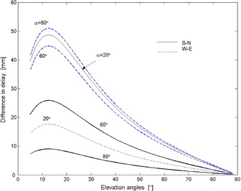
The difference in delays was calculated for a baseline length of 10 km, for both West-East (W-E) and South-North (S-N) baseline orientations. Three azimuth angles (α=20°, 60° and 80°) were investigated for these two baseline directions for 30 elevation angles ranging from 5° to 89° with an ionospheric profile of 67 TECU (1 TECU=1016 el.m−2) corresponding to local summer at equatorial region. The difference in ionosphere-induced delays is shown in Figure 1 for the S-N and W-E baseline directions. The relation between the baseline direction and the azimuth is most likely due to the different orientation of this line with regard to the satellite to receiver path.
Difference in delay for S-N and W-E baseline orientations of 10 km distance.

To model the ionospheric error correction for differential GPS (dGPS), these two figures are extremely useful in obtaining and understanding the relationship between the difference in delay and the difference in LOS as a function of the elevation angles. The relation between Δtd and ΔLOS for a given satellite position and their ratio:
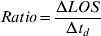
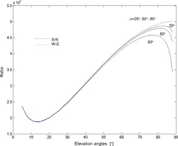
was determined for the two baseline orientations as a function of elevation angle (β). The ratio for the S-N direction is almost constant with azimuth at lower elevations but slightly dependent on azimuth at high elevations as shown in Figure 2. The difference in delay is actually higher at 20° azimuth for elevations less than 60° but so is ΔLOS. For the W-E direction, the ratio is almost constant at any azimuth angle. The ratios for both S-N and W-E baselines are approximately constant at any elevation angles (at least for elevations less than 60°). For a given azimuth, both Δtd and ΔLOS are approximately proportional to 1/cosβ. Results also show that the ratio is independent of the orientation of the baseline and the azimuth angle.
Ratio of group path.

The phase path shows similar results where the ratios are approximately the same for different azimuths at lower elevations but vary a little with azimuth at higher elevations although Δtd is less than 1 cm at these higher elevations. Furthermore, the difference between Δtd, g and Δtd, φ for dGPS is small (<0·05 mm) compared with that in the absolute value of group and phase at a single station so that either the group or phase path can be used to evaluate the ionospheric errors in dGPS. Both baselines located at mid-latitude and in the equatorial region show a similar variation of the ratio with elevation and dependence on the TEC value.
To facilitate correction for the difference in ionosphere-induced delay between the two paths, the ratio was modelled for a range of elevations from 10° to 60° (the range where the ionosphere-induced delay between the two paths is most pronounced). For example, this was done by fitting the ratio at 20° azimuth of the S-N direction determined from ray tracing by a 10th order polynomial function as defined in (2) as a function of elevation angle. This ratio is for the TEC of 44 TECU, a more realistic value for the temperate zone than that used in earlier work.

This function is almost constant at any baseline length as it was tested at 40 km baseline since the difference in the baseline length is normalised by including the ΔLOS. From (1) and (2), the difference in ionospheric delay at the reference station compared with the mobile station is given as:
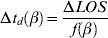
From this empirical equation, the difference in delay at any azimuth angle and at any baseline direction for a given reference station can be determined as long as ΔLOS is known. In practical relative positioning, this delay difference can be used directly in single difference processing between the receivers.
Horizontal gradients could also be included either by introducing linear gradients or by modelling the real latitudinal and longitudinal variation of the ionospheric electron density at all heights. In this work, however, only linear gradient was considered (Abdullah et al., Reference Abdullah, Strangeways and Walsh2003, Reference Abdullah, Strangeways and Walsh2007).
2.2. Variation of TEC and Profile Shape
In addition to the variation with elevation angle, the variation in TEC also affects the difference in delay between the two stations. To make the empirical model applicable at any location and for any TEC and geomagnetic conditions, the difference in delay due to differences of TEC and the profile shape was also investigated. To evaluate the TEC variation, one reference profile with 50 TECU was chosen and then scaled without changing the profile shape. The delay difference is about 1 mm for 20° elevation with an error of 1 TECU. To simplify the parameter fitting, instead of the ratio as in (1), the inverse ratio was plotted. Results show that the inverse ratio increases linearly with TEC and also goes to zero when the TEC is zero. So, for a given elevation angle, f(TEC)=(required TEC)/(TEC used in (2)) and then:

From (3) and (4), the difference in delay can be obtained from:

where:

which can be utilized for precise dGPS measurement.
The difference in delay due to differences of the profile shape was investigated using different profile shapes having the same TEC (50 TECU). The variation of delay difference with profile shape is not significant (~ sub-mm) and thus can be neglected for dGPS although it gives a small contribution for a single station measurement (Ioannides and Strangeways, op. cit.).
From the above results, ionospheric error correction can be made using the empirical formula including both elevation angle and TEC, which should be applicable to any location for accurate differential positioning.
3. EVALUATION OF THE MODEL
The developed model was evaluated using real GPS data recorded at differently spaced stations in the mid-latitude region. The parameters to be used in the model can be determined from several methods. For accurate results, the carrier phase (which is also affected by a significant ionospheric error) was primarily used instead of code pseudorange measurements. However, the integer ambiguity needs to be resolved. In doing so, short baseline measurements should be used but this might be corrupted with spatial disturbances such as travelling ionospheric disturbances or horizontal gradients. To overcome these irregularities, a long baseline and a magnetic undisturbed day are considered. The ambiguity can be resolved by using available software which offers various methods of ambiguity resolution. However, this depends on the availability of data recorded by the single or dual frequency receivers at suitably spaced stations. An example of implementing the model is also presented here by adding the model correction to data from reference station. The influence of the model can be examined by looking into its effect on the quality checking and on the carrier phase ambiguity resolution. As the surveyed true position is available, the estimated position with corrected measurements could be compared with this value.
3.1. Employing the model
Two main parameters, namely the difference in LOS and the TEC, need to be determined for this model.
3.1.1. ΔLOS
To obtain the LOS, the receiver and satellite positions should be known and there are several methods to obtain them. The receiver position can be used from a previously surveyed position or computed from navigation or observation data. In this work, the International GPS service (IGS) fixed positions were used as initial input to the calculation of the satellite position using broadcast ephemerides data. For comparison purposes the precise satellite position was also obtained from IGS precise ephemeris data. However, it was found that there is no significant difference between both methods as the difference in modelled differential ionospheric delay (Δtd) was sub-millimetre. So, either method can be used to obtain ΔLOS for the model.
3.1.2. TEC
Another essential parameter is the TEC and there are also several methods to obtain the TEC over the reference station. This depends on the required accuracy and the availability of the data. The simple but less accurate method is by using the Klobuchar model for single frequency where the required parameters are available from the ephemerides data. The TEC map can also be used either simulated from e.g. Bernese software, BGS, (Hugentobler, Reference Hugentobler, Schaer and Fridez2001) or downloaded from the IGS website. In this work TEC was obtained from the IGS TEC map and from the standard dual frequency method. Even though there is a significant difference (average of 8 TECU) between the TEC computed from each method, it only contributes to about 6% of the maximum value. This shows that the TEC accuracy is not that crucial and either method can be used.
It should be noted that IGS precise position and TEC map data is not available in real time but with latency of approximately one week (IGS, 2005).
3.2. Evaluating the model with real data
In order to evaluate the model, real GPS measurements were obtained from the IGS stations Brussels (50·8°N, 4·7°E), BRUS, and Zimmerwald (46·9°N, 7·5°E), ZIMM, on 5 August 2002. The longer baseline distance of approximately 500 km was used (BRUS-ZIMM) to overcome the spatial irregularities. Four other stations were added to make a network centred at BRUS. These nearby stations produce more measurements and therefore aid in the parameterisation. The integer ambiguity was resolved and the data was then processed using BGS software to get the absolute differential delay. The differential error from this real data was investigated and dominated by the effects of ionospheric effects rather than the multipath and noise.
Even though the TEC is slowly varying over this baseline, it still results in significant differential delay, especially at low elevation angles. The delay due to the gradients could be added or subtracted from the modelled differential delay depending on the propagation path and the baseline direction above. For the BRUS-ZIMM baseline, the propagation path was affected by the latitudinal gradients at low elevation angles. Then the latitudinal gradients were included with reference to the IRI-2001 ionospheric model. It was found that ionospheric differential delay of a real data is in a good agreement with the modelled differential delay.
4. APPLICATION OF THE MODEL
The differential delay correction can be applied either at the reference or mobile station. The corrected range of phase L1 single difference measurements between reference station A and mobile station B, without considering the ambiguity term is given as:

where
φA, φB: phase measurements in unit of cycles of stations A and B
IA, IB: ionospheric error experienced by both paths
Δtd: differential delays between the stations in unit of cycles
With reference to (5), the correction model is determined by a function of two variables of the particular satellite observed at both stations. It is controlled by the elevation angles at particular epochs and correction should be applied for low elevation angles of less than 60°. The second controlling factor, the TEC, can be obtained from line of sight TEC experienced by the satellite-receiver path epoch by epoch.
In current practice, the correction is calculated at the reference station, transmitted to the mobile station, and then applied. Here, in this preliminary application and investigation, the approach taken was to apply the differential correction by modifying the carrier phase measurements as in (6). The TEC over the reference station was computed from the observation data using the dual frequency model and the elevation angle was computed from navigation data at the reference station. The difference in LOS was computed from the navigation data of both stations. The TEC and LOS could alternatively be obtained from other sources described earlier. Using these parameters as an input, the differential correction was computed and applied to the reference station L1 measurements. The corrected observation files in RINEX format (Gurtner, Reference Gurtner2001) were then used in the processing. GPSurvey software (Trimble, 1994) was used to process both corrected and uncorrected measurements. The broadcast ephemeredes was used, and to avoid estimated position with poor geometry, GDOP (geometric dilution of precision) smaller or equal to 6 was used. The Hopfield tropospheric correction model was used instead of measured meteorological data. The elevation mask was set to 10° and the L1 fixed double difference solution was used as the final solution but no ionospheric correction was used from the software.
In the GPSurvey software, there are two quality indicators to evaluate the processing results after the ambiguity is resolved. They are generated from the statistical results of the observation used as:
• Variance ratio: This is applied for fixed solutions only. From the integer ambiguity search, variances can be determined. The software processors rank the variances where the lowest is the best variance. The second lowest is the next best variance. The variance ratio is the ratio of the second best over the first best. A higher variance ratio is favoured and generally, it is more than 1·5 for a valid fixed solution.
• Reference variance: This value indicates how well the observed data fit into the computed solution. A value of 1 up to 10 is acceptable for kinematics and single frequency measurements, for example a 30 km L1 single frequency baseline may result in a reference variance of 10 to 20 or more due to ionospheric errors (ibid). A short period such as 5 minutes may also have high variance due to multipath effects. Lower variance implies more precision.
Both the ratio and the variance distribution can be controlled by the specific level of confidence, which was set to be 95%.
There are several parameters from the summary report of GPSurvey output that can be examined to evaluate the influence of the correction model. They are:
— the estimated position of the mobile station
— the standard deviation of position or baseline components
— ambiguity resolution rate and
— the variance ratio and reference variance of the processing solution
Applying the correction model into the phase measurements should deliver better ranges. This can be evaluated by examining the above parameters that should give:
— better position; the computed position can be compared with the true position, if it is available
— the standard errors of position or baseline components are smaller
— ambiguity can be resolved in shorter period and
— if the ambiguity is resolved, the variance ratio is larger and the reference variance is smaller
Then the influence of the correction was examined from the quality check resulting from the data processing and its effect on carrier phase ambiguity resolution errors. The standard deviation of baseline component in local geodetic coordinate system, North, East and Up was also compared.
4.1. Evaluation of ambiguity resolution rate
The observation data was taken from Glasgow (55·9°N, 4·3°E), GLAS, and Stirling (56·1°N, 4·1°E), STI1, on 13 August 2002. Glasgow was assumed as a reference station and Stirling was a mobile station giving a baseline of about 28 km. Even though dual frequency data are available on both stations, only single frequency L1 measurements were used for positioning. This is the most critical condition where only single frequency receivers, which are mostly affordable in developing countries, are available. The data quality was initially checked using TEQC (i.e. the multipath noise) (Estey and Meertens, Reference Estey and Meertens1999). The pseudorange multipath is 0·21 m for Glasgow and 0·33 m for Stirling. Since it is hard to determine the phase multipath that could be only millimetric, where the multipath effect on the phase is two orders of magnitude less than that on the code (Seeber, Reference Seeber2003), the results obtained are contaminated with multipath. According to Leick (Reference Leick2004) the multipath effect for short baseline was likely cancelled in the single difference observables used in this work. The multipath effects were also checked using technique suggested by Georgiadou and Kleusberg (Reference Georgiadou and Kleusberg1988), and Wanninger and May (Reference Wanninger and May2000), showing that the multipath effect is small. Furthermore, the stations were well sited and are run by established organizations and therefore, should have less noise; so, it was assumed that the multipath effects induced in the measurements are small.
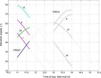
Figure 3 shows some of the satellite elevation angles. The first 5 solid lines in the figure show a specific duration of 40 minutes (161 propagation paths with 15 seconds interval for every epoch). This is the duration for which the ionospheric correction was applied. A shorter time was chosen to see how this correction influences the ambiguity resolution. The ambiguity can be resolved for longer periods without applying any ionospheric correction. Within the 40-minute period from 11:00:00 to 11:40:00, the observed satellites PRNs are 1, 4, 13, 24, and 27 from both stations. The model was evaluated by firstly applying the correction to the PRN27 measurements, then applying it to both the 27 and 24 measurements (because both satellites were seen at low elevation angles at the earlier epochs), and finally by applying it to the 27, 24, 01 and 04 measurements together. PRN13, on the other hand, is a reference satellite at high elevation angles.
Satellite elevation angles.

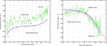
In applying the model, the TEC was computed from observation measurements using the dual frequency method considering every epoch for the specific satellites. By doing this, the actual TEC experienced by the propagation path is used instead of the weighted values of TEC from several satellites paths obtained from a TEC map. The TEC over Glasgow at that 40-minute duration is about 15 to 20 TECU, which can be considered as a medium TEC values for mid-latitude region. The differential delays computed from the model for PRN27 and 24 are shown in Figure 4. The differential delay obtained from the L4 residual was plotted in the same figure where it was scaled to L1 and with the ambiguity eliminated. Since the differential delay obtained from the measurements was noisy, a fitted value was plotted. The model, however, cannot be evaluated by looking at the delay difference from the real measurements because the ambiguity was not resolved. The modelled differential delay shows a good agreement in terms of its pattern (the delay difference with variation of time) with the measured values for both figures. The differential delay of satellite PRN27 is about 2 cm whereas for PRN24 (that was observed at higher elevation angles) is less than 1 cm.
Differential delay computed from the model and L4 residual (PRN27&24). Left – Diff delay scaled to L1 of PRN27. Right – Diff delay scaled to L1 of PRN24.

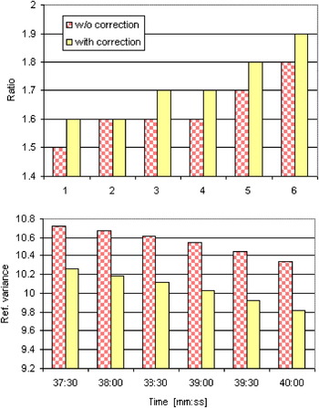
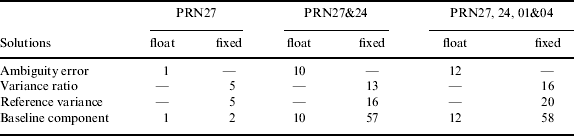
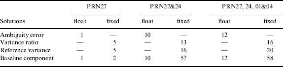
When the processing cannot resolve the ambiguity, it produces a float solution non-integer ambiguity estimate. Whereas, when the processing can resolve the ambiguity to a correct integer number, it results in a fixed solution. With these 4 satellites, (uncorrected data) the ambiguities were resolved with the occupation time of 11:37:30. By applying the correction model to PRN27, ambiguities were resolved at 11:36:30, which is 1 minute earlier corresponding to a reduction of 4 epochs. The deviation of rounded values of the float ambiguities cannot be compared because the fixed value of ambiguity is not available from the software. However, the improvement can be seen by comparing the variance ratio, reference variance and estimated position errors of the processing after the ambiguities were resolved. For example, the ratio in Figure 5 increases while the reference variance decreases indicating the improvement in the processing results. The difference gives an average of 5% improvement in the ratio and the reference variance compared to uncorrected measurements. To see how this improvement influences the estimated position, the standard deviations of local position of North, East and Up were compared with corrected measurements. Results show the standard deviations improve by about 2% and a trend of increasing improvement with time. Of course the improvement increases with the correction applied to most satellites measurements. The ambiguity was resolved at 11:35:00, which is 2·5 minutes faster than without the correction, after PRNs 27, 24, 01 and 04 measurement were corrected. Significant improvements were obtained with an average of 16% and 20% for the ratio and the reference variance respectively. Meanwhile the East, North, and Up components improve on average by 71%, 59% and 45%, respectively.
Comparison of variance ratio and reference variance with corrected measurements of PRN27.

Table 1 summarises the ambiguity resolution success rate without and with the correction applied and Table 2 summarises the percentage of average improvements with the corrected measurements.
Ambiguity resolution success rate.

Percent improvement with the corrected measurements.
4.2. Measurements corrected for significant differential delay
In the previous case, the corrected measurements were found not to have brought about much of an improvement when the estimated position was compared with the true position. This might be due to the short period of time that was taken soon after the ambiguities were resolved and the small differential ionospheric delays between the stations of less than 2 cm in all four satellite measurements. The measurements were then further corrected with higher differential delays. A significant increase in differential delay of PRN24 of about 1·5 cm to 5·5 cm can be seen in Figure 4 (Right) from the 13th to 14th hour. This one-hour period of data was taken to evaluate the correction method and was compared with the quality of processing solution and true position as the above process. Figure 3 also shows the elevation angles for the satellites (PRN10, 8, 24 27) seen from both stations and used in this processing. PRN10 was a reference satellite with elevation angles of 59° to 74°. Even though PRN27 can be seen at an elevation angle of 45° at 14th hour, it only contributes to about 4 mm of differential delay (see Figure 4 (Left)). Therefore, only PRN24 measurements with elevation angles from about 40° to 15° were corrected in this processing.
4.2.1. Evaluation of corrected data with estimated position
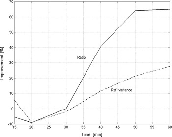
The ambiguities were resolved at about the same time, at 13:14:15, for both uncorrected and corrected measurements. This is likely due to all the measurements being less affected by the ionosphere for elevation angles of more than 40°. Both ratio and reference variances show little difference between uncorrected and corrected measurements until after 40 minutes of processing. This is when the differential delay is about 4 cm for PRN24. Then the ratios for the corrected measurements increase sharply and show about 40% improvement as shown in Figure 6. The improvement in ratio increases to about 65% at 60 minutes. In contrast, the reference variance at first shows a decrease for the corrected measurements. However, it contributes to about 28% improvement after 60 minutes of processing.
Improvement in the ratio and reference variance after PRN24 measurements were corrected for 1 hour.

4.2.2. Evaluation of corrected data with true position
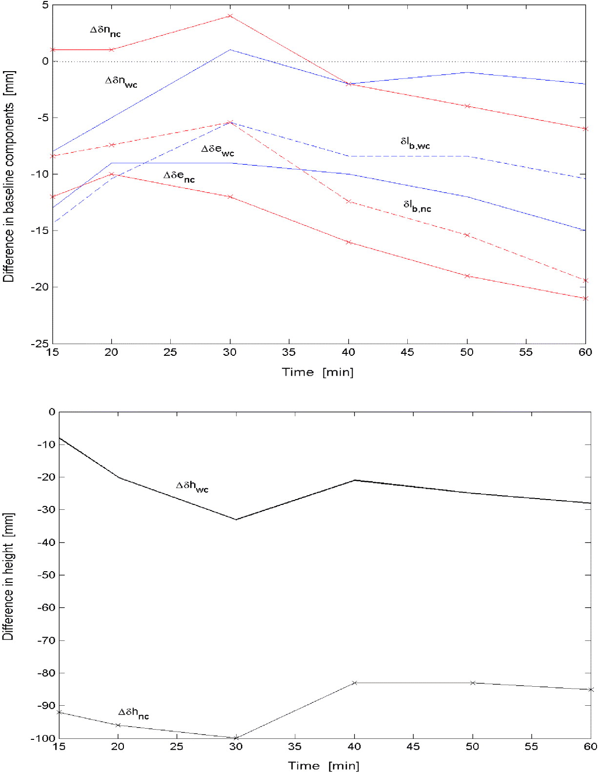
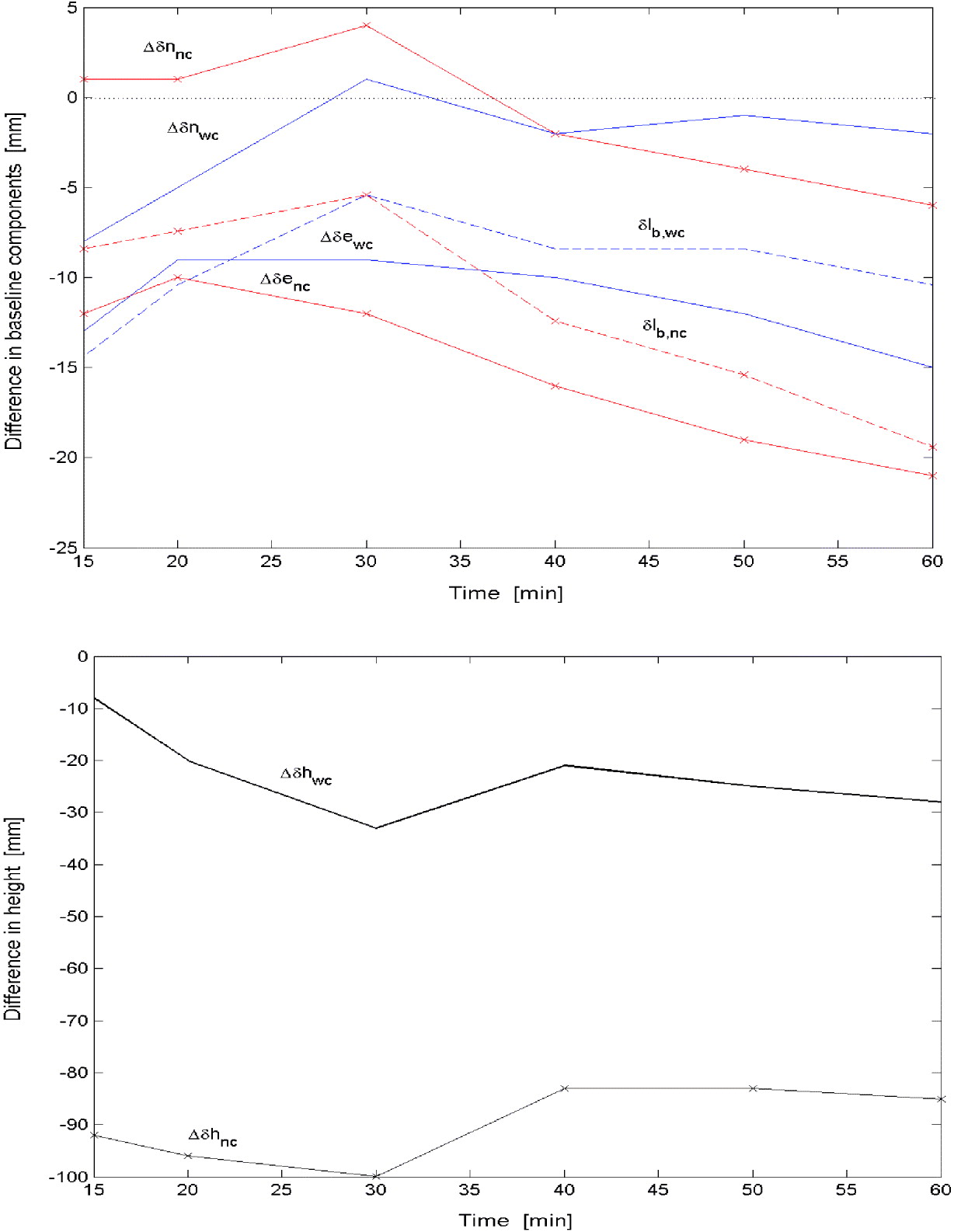
Again the estimated processing solutions show encouraging results. The estimated position was then compared with the true position using the United Kingdom national grid system. STI1 is located at 15511·999 m easting, 23725·489 m northing and 425·675 m height away from GLAS with a baseline distance of 28354·669 m. The estimated baseline components with uncorrected and corrected measurements were compared with the true baseline components of easting (e), northing (n) and height (h). The differences in baseline components are shown in Figure 7. The uncorrected measurements were marked whereas the corrected measurements were not. The differences in baseline components of easting (Δ δe) and northing (Δ δn) are shown in Figure 7 (Top) and, since the difference in the height component (Δ δh) was much larger, it is shown separately in Figure 7 (Bottom), for comparison. In these figures, subscripts nc and wc denote uncorrected and corrected measurements respectively. Both uncorrected and corrected measurements do not vary monotonically with increasing time, especially around 30 minutes. After 40 minutes, all corrected measurements show some improvements. Comparison at 60 minutes is discussed next. For the northing component, the estimated values are in error by 6 mm for Δ δnnc and by 2 mm for Δ δnwc, showing significant improvement of about 67%. For the easting component, they are in error by 21 mm and 15 mm for Δ δenc, and Δ δewc respectively, improving by about 29%. While for the height component, the estimated values are in error by 85 mm and 28 mm for Δ δhnc, and Δ δhwc respectively, showing a significant improvement of 67%. The baseline distance (lb), superimposed in Figure 7 (Top) is in error by 19 mm for δlb,nc and by 10·4 mm for δlb,wc, which shows about 45% improvement. Overall, an average improvement of easting, northing and height is about 54% when approximately 5·5 cm differential delay was corrected at 60 minutes. Other error sources that were not fully eliminated or corrected during the processing might still be contaminating the measurements. However, the estimated position shows good agreement with the true position.
Comparison with true position with PRN24 corrected measurements. (Top) Difference in baseline components with true position. (Bottom) Difference in height with true height.
5. CONCLUSION
The results show an improvement in the correction of the differential ionospheric error over short and medium baselines. For longer baseline, ionospheric gradients should be considered. Although still preliminary, by applying the corrected model, the obtained results compared to uncorrected measurements have indicated that the ambiguity success rate is faster even when only correcting one satellite seen at low elevation angles. This success rate increases by correcting other satellite paths. After the ambiguities are resolved, the variance ratio is larger and the reference variances are smaller. This implies good processing results. When a longer period was used after the ambiguities were resolved, and significant differential delay (about 5 cm) was corrected, all baseline components showed improvement of more than 50% on average compared to the true position. This shows an encouraging improvement. However, further studies to improve L1 relative positioning should be performed, aiming to fully eliminate the differential ionospheric delay.
In general, it is hoped that this developed model will give a significant contribution to radio propagation by introducing a better ionospheric model for precise positioning including short and medium baselines. The application of this model can give better GPS surveying results for single frequency receivers. In addition, the proposed method could be extended for global and wide area ionosphere estimation if electron density gradients (ionosphere model with 3-D electron density gradients) become available and therefore, some improvement could be made.
ACKNOWLEDGEMENTS
The services of the Natural Environment Research Council (NERC) British Isles GPS archive Facility (BIGF), www.bigf.ac.uk, and International GPS Service (IGS), igscb.jpl.nasa.gov, are gratefully acknowledged, for providing archived GPS data for this project.