2 Governing equations

We consider a buoyancy driven flow in an infinitely long and weakly curved vertical channel. A concise derivation of the equations and explanation of the key points of our model is presented in this section. Full details are given in appendix A. The derivation of the governing equations for this configuration is analogous to that for heated curved pipes, presented in Yao & Berger (Reference Yao and Berger1978).

The steady NS equations, coupled with the steady heat equation govern the velocity, $\boldsymbol{u}$ , pressure, $p$ , and temperature, $T$ . These are given by

(2.1) $$\begin{eqnarray}\displaystyle & \displaystyle \unicode[STIX]{x1D735}\boldsymbol{\cdot }\left(\unicode[STIX]{x1D70C}\boldsymbol{u}\right)=0, & \displaystyle\end{eqnarray}$$

(2.2) $$\begin{eqnarray}\displaystyle & \displaystyle \unicode[STIX]{x1D70C}\boldsymbol{u}\boldsymbol{\cdot }\unicode[STIX]{x1D735}\boldsymbol{u}=-\unicode[STIX]{x1D735}p+\unicode[STIX]{x1D70C}\boldsymbol{g}+\unicode[STIX]{x1D707}\unicode[STIX]{x1D6FB}^{2}\boldsymbol{u}, & \displaystyle\end{eqnarray}$$

(2.3) $$\begin{eqnarray}\displaystyle & \displaystyle \boldsymbol{u}\boldsymbol{\cdot }\unicode[STIX]{x1D735}T=\unicode[STIX]{x1D705}\unicode[STIX]{x1D6FB}^{2}T, & \displaystyle\end{eqnarray}$$

where $\unicode[STIX]{x1D70C}$ is the density, $\boldsymbol{g}$ the acceleration of gravity, $\unicode[STIX]{x1D707}$ the dynamic viscosity and $\unicode[STIX]{x1D705}$ the thermal diffusivity.

Figure 1.

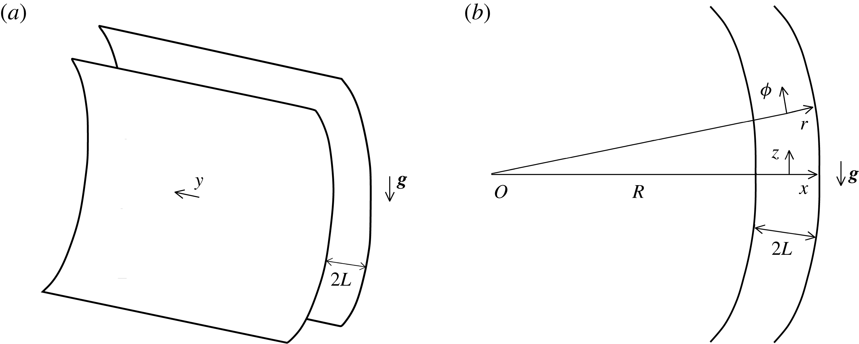
Depiction of curved channel. Gravity acts in the negative $z$ direction and $y$ is in the transverse direction. On the right we indicate the cylindrical and Cartesian reference frames. The width of the channel is $2L$ , and the radius of curvature $R$ , are such that $L\ll R$ .

We consider a cylindrical coordinate system $(r,\unicode[STIX]{x1D719},y)$ , as depicted in figure 1, where the curvature is greatly exaggerated. We have that $y$ is in the transverse direction, $r$ is across the gap, and $\unicode[STIX]{x1D719}$ along the channel. The length scales are the width of the gap $2L$ , and the radius of curvature $R$ . The geometry is unbounded in the $y$ direction. We assume that the channel is very weakly curved, so that, to leading order, gravity only acts in the negative $\unicode[STIX]{x1D719}$ direction. Furthermore, we assume fully developed flow in this direction, thus independent of $\unicode[STIX]{x1D719}$ . We employ the Boussinesq assumption (Boussinesq Reference Boussinesq1897), so that density variations are only important in the gravitational term. We also make the Dean approximation (Dean Reference Dean1927), regarding the channel curvature, $\unicode[STIX]{x1D706}=2L/R$ , as small, and neglect terms of $O(\unicode[STIX]{x1D706})$ . Once all assumptions are taken into account, the system of equations can be described in the local Cartesian reference frame $(x,y,z)$ , depicted in figure 1. We also make the equations non-dimensional (details in appendix A). The following nomenclature is adopted,

(2.4) $$\begin{eqnarray}\boldsymbol{u}=\left(\frac{\unicode[STIX]{x2202}\unicode[STIX]{x1D713}}{\unicode[STIX]{x2202}y},-\frac{\unicode[STIX]{x2202}\unicode[STIX]{x1D713}}{\unicode[STIX]{x2202}x},w\right),\end{eqnarray}$$

where $\unicode[STIX]{x1D713}$ is a streamfunction, and $w$ the velocity component in $z$ . We adopt $\unicode[STIX]{x1D703}$ as the non-dimensional temperature. Taking all assumptions into account, we obtain the thermally modified Dean equations

(2.5) $$\begin{eqnarray}\displaystyle & \displaystyle {\mathcal{J}}(w,\unicode[STIX]{x1D713})=\unicode[STIX]{x1D6FB}^{2}w+G\unicode[STIX]{x1D703}, & \displaystyle\end{eqnarray}$$

(2.6) $$\begin{eqnarray}\displaystyle & \displaystyle {\mathcal{J}}(\unicode[STIX]{x1D6FB}^{2}\unicode[STIX]{x1D713},\unicode[STIX]{x1D713})=\unicode[STIX]{x1D6FB}^{4}\unicode[STIX]{x1D713}+2w\frac{\unicode[STIX]{x2202}w}{\unicode[STIX]{x2202}y}, & \displaystyle\end{eqnarray}$$

(2.7) $$\begin{eqnarray}\displaystyle & \displaystyle {\mathcal{J}}(\unicode[STIX]{x1D703},\unicode[STIX]{x1D713})=Pr^{-1}\unicode[STIX]{x1D6FB}^{2}\unicode[STIX]{x1D703}, & \displaystyle\end{eqnarray}$$

where

(2.8) $$\begin{eqnarray}{\mathcal{J}}(A,B)=\frac{\unicode[STIX]{x2202}A}{\unicode[STIX]{x2202}x}\frac{\unicode[STIX]{x2202}B}{\unicode[STIX]{x2202}y}-\frac{\unicode[STIX]{x2202}A}{\unicode[STIX]{x2202}y}\frac{\unicode[STIX]{x2202}B}{\unicode[STIX]{x2202}x},\end{eqnarray}$$

and

(2.9a,b ) $$\begin{eqnarray}G=\frac{g\unicode[STIX]{x1D6FD}\unicode[STIX]{x0394}TL^{3}}{\unicode[STIX]{x1D708}^{2}}\left(\frac{L}{R}\right)^{1/2},\quad Pr=\frac{\unicode[STIX]{x1D708}}{\unicode[STIX]{x1D705}},\end{eqnarray}$$

i.e. $G$ is proportional to the Grashof number and the square root of the curvature, $Pr$ is the Prandtl number, $\unicode[STIX]{x1D708}$ the kinematic viscosity. The resulting system of equations is essentially the thermally coupled NS equations in two dimensions, with a centrifugal body force acting towards the inside wall.

These equations are valid for any buoyancy driven flow in a weakly curved channel. We now particularise to flow driven by a linearly varying temperature gradient, by imposing at the walls

(2.10) $$\begin{eqnarray}\unicode[STIX]{x1D703}(\pm 1,y)=\pm y,\end{eqnarray}$$

where the inner and outer wall are located, respectively, at $x=-1$ and $x=1$ . We seek solutions linear in $y$ , assuming $w(x,y)={\hat{w}}(x)y$ , $\unicode[STIX]{x1D703}(x,y)=\hat{\unicode[STIX]{x1D703}}(x)y$ , $\unicode[STIX]{x1D713}(x,y)=\hat{\unicode[STIX]{x1D713}}(x)y$ . Dropping the hats, the system of equations becomes

(2.11) $$\begin{eqnarray}\displaystyle & \displaystyle w^{\prime }\unicode[STIX]{x1D713}-w\unicode[STIX]{x1D713}^{\prime }=w^{\prime \prime }+G\unicode[STIX]{x1D703}, & \displaystyle\end{eqnarray}$$

(2.12) $$\begin{eqnarray}\displaystyle & \displaystyle \unicode[STIX]{x1D713}^{\prime \prime \prime }\unicode[STIX]{x1D713}-\unicode[STIX]{x1D713}^{\prime \prime }\unicode[STIX]{x1D713}^{\prime }=\unicode[STIX]{x1D713}^{\prime \prime \prime \prime }+2w^{2}, & \displaystyle\end{eqnarray}$$

(2.13) $$\begin{eqnarray}\displaystyle & \displaystyle \unicode[STIX]{x1D703}^{\prime }\unicode[STIX]{x1D713}-\unicode[STIX]{x1D703}\unicode[STIX]{x1D713}^{\prime }=Pr^{-1}\unicode[STIX]{x1D703}^{\prime \prime }, & \displaystyle\end{eqnarray}$$

where the primes denote derivatives with respect to $x$ . Our variables $w$ , $\unicode[STIX]{x1D713}$ and $\unicode[STIX]{x1D703}$ are functions of $x$ only, as now our solutions are self-similar in $y$ .

We also wish to impose no-slip condition on the walls, thus, our complete set of boundary conditions is

(2.14a,b ) $$\begin{eqnarray}w=\unicode[STIX]{x1D713}=\unicode[STIX]{x1D713}^{\prime }=0,\quad \unicode[STIX]{x1D703}=\pm 1\quad \text{at }x=\pm 1.\end{eqnarray}$$

We have assumed that, to leading order, gravity only acts in the negative $z$ direction. A fairly simple extension of this work would be to consider an inclined channel. This requires gravity to have components in the $x$ - and $z$ - directions. We derive this system in appendix B. However, as the dominant characteristics of the flow are unchanged, we do not consider the channel inclination further.

3 Extended Stokes series

We shall solve the system numerically in § 5, but it is useful first to obtain an analytical representation of the solution by expanding the variables in powers of $G$ ,

(3.1a-c ) $$\begin{eqnarray}w=\mathop{\sum }_{n=0}^{\infty }w_{n}G^{n},\quad \unicode[STIX]{x1D703}=\mathop{\sum }_{n=0}^{\infty }\unicode[STIX]{x1D703}_{n}G^{n},\quad \unicode[STIX]{x1D713}=\mathop{\sum }_{n=0}^{\infty }\unicode[STIX]{x1D713}_{n}G^{n}\end{eqnarray}$$

and truncate at $N$ coefficients. The leading-order coefficients are given by the straight channel solution, $w_{0}=0$ , $\unicode[STIX]{x1D713}_{0}=0$ , $\unicode[STIX]{x1D703}_{0}=x$ and $w_{1}=(x-x^{3})/6$ . We can derive recurrence relations to compute higher-order coefficients of the series. For example, for $\unicode[STIX]{x1D703}$ we have

(3.2) $$\begin{eqnarray}\unicode[STIX]{x1D703}_{n}^{\prime \prime }=\mathop{\sum }_{i,j:i+j=n}Pr(\unicode[STIX]{x1D703}_{i}^{\prime }\unicode[STIX]{x1D713}_{j}-\unicode[STIX]{x1D703}_{i}\unicode[STIX]{x1D713}_{j}^{\prime }),\end{eqnarray}$$

which we can use to determine

(3.3) $$\begin{eqnarray}\unicode[STIX]{x1D703}_{2}=\frac{1}{59875200}Pr(x^{2}-1)(45x^{10}-263x^{8}+562x^{6}+562x^{4}-703x^{2}-5323).\end{eqnarray}$$

The series coefficients are polynomials in $x$ and $Pr$ . We find that the $\unicode[STIX]{x1D713}$ and $\unicode[STIX]{x1D703}$ series are even in $G$ , while the $w$ series is odd.

By computing the series coefficients using recurrence relations, our nonlinear system reduces to a sequence of linear problems. Naturally, it becomes increasingly computationally expensive to compute higher-order coefficients. We have used the software MAPLE to compute up to $N=236$ coefficients of the series.

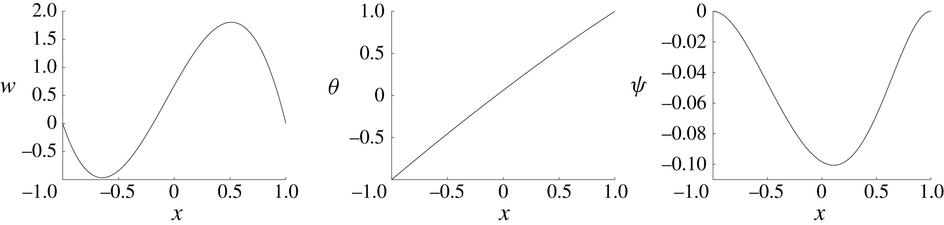
The velocity and temperature fields for $Pr=1.1$ and $G=21$ are presented in figure 2. We recall that the fluid velocity is $\boldsymbol{u}=(\unicode[STIX]{x1D713},-y\unicode[STIX]{x1D713}^{\prime },yw)$ and the temperature is $y\unicode[STIX]{x1D703}$ . We can see that for $y>0$ , the inner wall is cold and the fluid sinks ( $\unicode[STIX]{x1D703}<0,w<0$ ), whereas it rises by the warm, outer wall. For this moderate value of $G$ , the temperature profile is almost linear. As $\unicode[STIX]{x1D713}<0$ , we see that the $x$ -velocity is always towards the inner wall. Fluid then departs the inner wall in the positive and negative $y$ -directions. The outer wall behaviour is reversed.

Figure 2.

Velocity and temperature profiles for $Pr=1.1$ and $G=21$ . We see $w<0$ close to the inner wall which is cold for $y>0$ , whereas $w>0$ near the outer (hot) wall. The temperature profile is approximately linear. The $x$ -velocity is towards the inner wall, for all $y$ , as $\unicode[STIX]{x1D713}<0$ .

3.1 Limits of validity

This solution is only valid inside the radius of convergence of the series, $G_{c}$ , which is limited by the nearest singularity in the complex $G$ -plane (Van Dyke Reference Van Dyke1974). We can estimate $G_{c}$ , using a Domb–Sykes plot, following Domb & Sykes (Reference Domb and Sykes1957). In case of an algebraic singularity $(G-G_{c})^{\unicode[STIX]{x1D6FC}}$ , the ratios of consecutive coefficients of a series $\sum c_{n}G^{n}$ , should be linear in $1/n$ , for large $n$

(3.4) $$\begin{eqnarray}\frac{c_{n}}{c_{n-1}}=\frac{1}{G_{c}}\left(1-\frac{1+\unicode[STIX]{x1D6FC}}{n}+O\left(\frac{1}{n^{2}}\right)\right).\end{eqnarray}$$

All measures of the series solution will have the same value of $G_{c}$ . For this discussion we chose to compute the ratios of $\unicode[STIX]{x1D713}$ at $x=0.5$ , which we refer to as,

(3.5) $$\begin{eqnarray}f(G)=\mathop{\sum }_{n=2}^{N}c_{n}G^{n}.\end{eqnarray}$$

Since the series is even, we started by computing the ratios $c_{n}/c_{n-2}$ . However, this Domb–Sykes plot alternated between two lines, indicating that we should consider instead the ratios $c_{n}/c_{n-4}$ . We find that the singularity is of the type $f(G)\sim (G_{c}^{4}-G^{4})^{1/2}$ , which corresponds to four singularities $\{\pm G_{c},\pm iG_{c}\}$ . As one of these values is real and positive, this suggests that a solution branch will turn at $G=G_{c}$ . We will observe later that the first fold in the bifurcation diagram indeed occurs at $G_{c}$ .

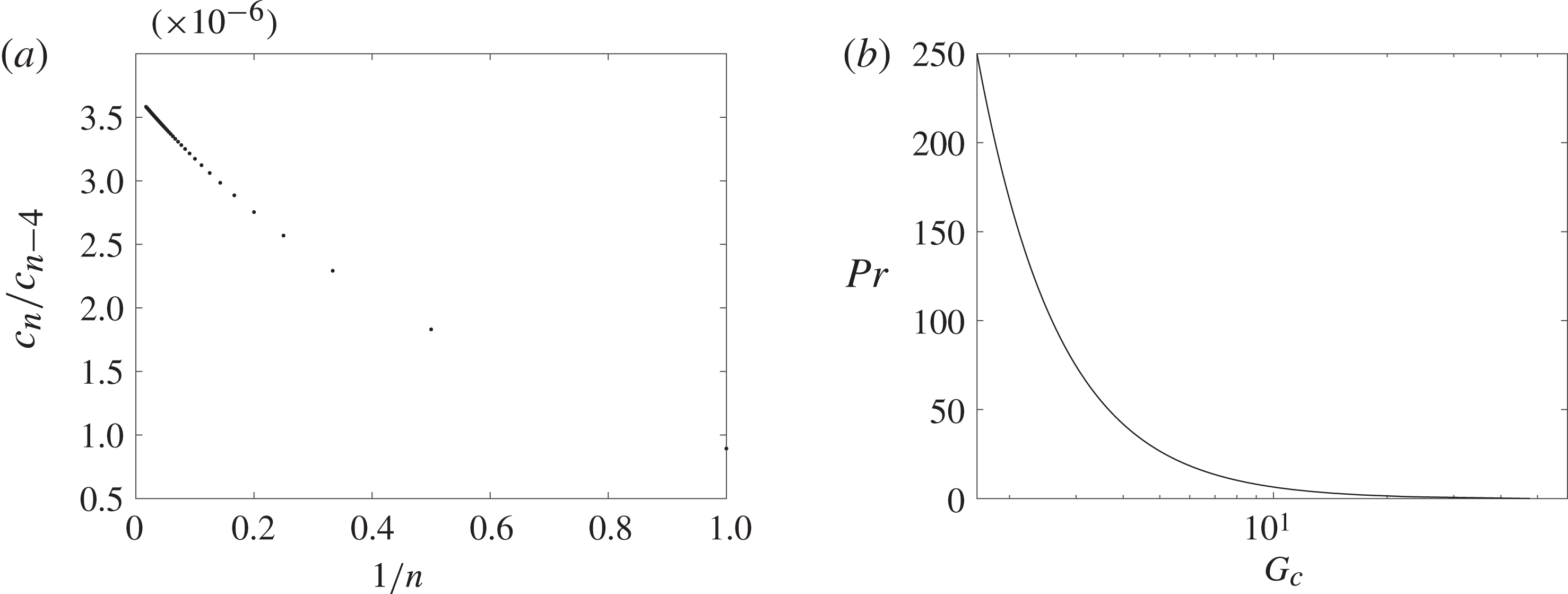
For $Pr=1$ the Domb–Sykes plot is presented in figure 3. Using polynomial extrapolation we find that $G_{c}\simeq 22.8$ . The value of $G_{c}$ for different values of $Pr$ can be observed in figure 3. For $Pr=0$ we find $G_{c}\simeq 44.7$ . Furthermore, as $Pr\rightarrow \infty$ we observe that $G_{c}\sim Pr^{-1/2}$ .

Figure 3.

(a) Domb–Sykes plot for $Pr=1$ . Since the ratios of the coefficients are positive, this indicates a real singularity in the complex $G$ -plane which anticipates a turning point at $G=G_{c}$ . As $n\rightarrow \infty$ the ratio approaches $G_{c}^{-4}$ . (b) $G_{c}$ for different values of $Pr$ . We observe that $G_{c}\sim Pr^{-1/2}$ as $Pr\rightarrow \infty$ .

4 Analytic continuation by high-order Hermite–Padé approximants

In this section we explore a method to bypass the limitation of our series solution and extend our analysis to higher parameter values by means of generalised Hermite–Padé approximants. This method was implemented in Boshier & Mestel (Reference Boshier and Mestel2014, Reference Boshier and Mestel2017), and is introduced and described in detail in Drazin & Tourigny (Reference Drazin and Tourigny1996). The key points of the method are as follows. From a series expansion

(4.1) $$\begin{eqnarray}U_{N}(G)=\mathop{\sum }_{n=1}^{N}c_{n}G^{n}+O(G^{N+1}),\end{eqnarray}$$

we construct a polynomial,

(4.2) $$\begin{eqnarray}F_{d}(u,G)=\mathop{\sum }_{m=1}^{d}\mathop{\sum }_{k=0}^{m}f_{m-k,k}G^{m-k}u^{k}=0,\end{eqnarray}$$

where the coefficients $f_{i,j}$ , are computed such that $u=U_{N}$ is a solution to (4.2). The maximum order of the approximant, $d$ , is determined by how many coefficients of the series are available. In order to ensure that the number of unknown coefficients $f_{i,j}$ equals the number of equations, we truncate $u$ at $N$ where,

(4.3) $$\begin{eqnarray}N={\textstyle \frac{1}{2}}(d^{2}+3d-2).\end{eqnarray}$$

The main advantage of this method is the possibility of finding multiple solution branches. For each order $d$ of the approximant a polynomial is constructed and its roots for a certain $G$ value yield $d$ solutions. Some of these roots are spurious, but we can track actual flow solutions as they appear consistently as the order $d$ is increased.

Figure 4.

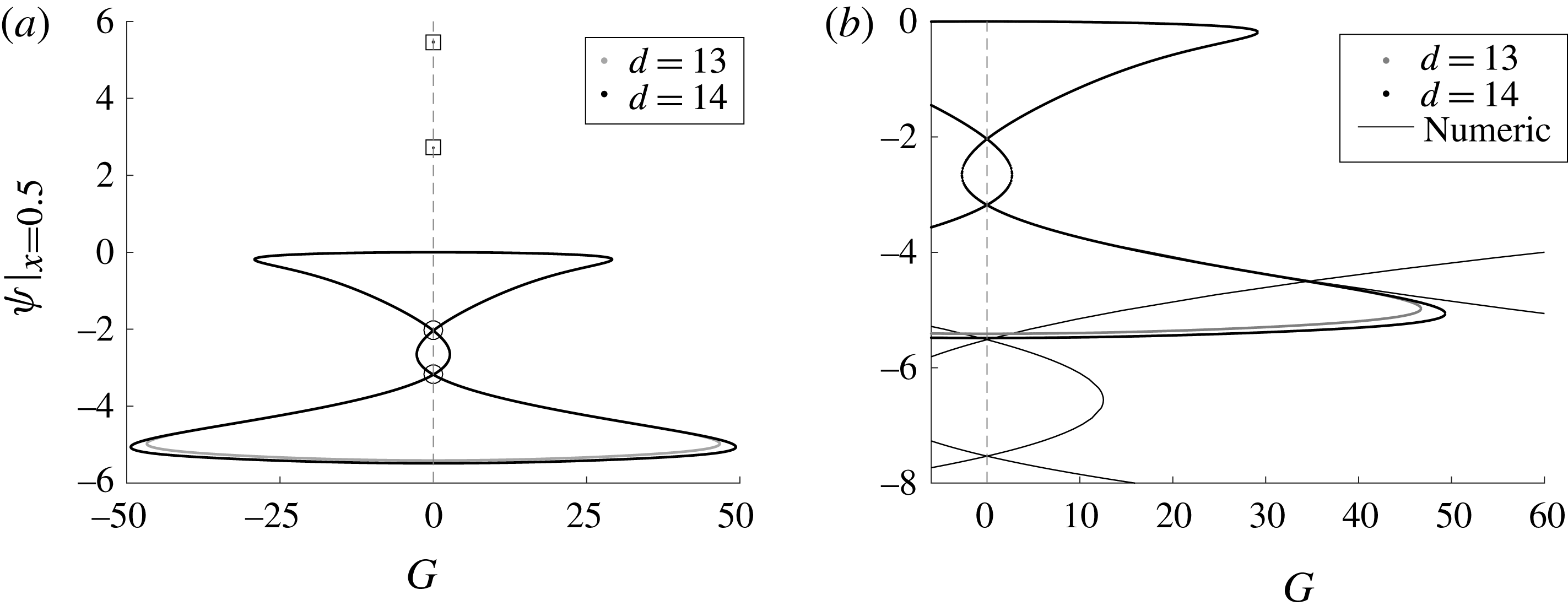
(a) Bifurcation diagram for $Pr=0.5$ , the selected measure is $\unicode[STIX]{x1D713}(0.5)$ . The approximants for $d=13$ and $d=14$ are shown. The solutions are multivalued and symmetric in $G$ . Non-trivial solutions for $G=0$ are highlighted with squares for positive $\unicode[STIX]{x1D713}$ , and circles for negative values. (b) Comparison between analytical continuation and numerical results. The latter allows us to extend the bifurcation diagram and reveals two additional unforced solutions.

The highest order of approximant that we have obtained is $d=14$ . In figure 4, we observe a typical bifurcation diagram. The case considered is $Pr=0.5$ and the measure selected is $\unicode[STIX]{x1D713}(0.5)$ . We show the results obtained with approximant order $d=13$ and $d=14$ . In the interest of clarity we omit spurious solutions. Many interesting aspects of the solution are revealed. First we note the symmetry of the solution branches about $G=0$ . This occurs as the system of (2.11)–(2.13) is invariant under the transformation $G\rightarrow -G$ , $w\rightarrow -w$ , $\unicode[STIX]{x1D713}\rightarrow \unicode[STIX]{x1D713}$ and $\unicode[STIX]{x1D703}\rightarrow \unicode[STIX]{x1D703}$ . Secondly, we observe three turning points, the first at $G\simeq 29.1$ corresponds to the value predicted by Domb–Sykes analysis, and two more. One at $G\simeq 2.7$ , and the last one apparently at $G\approx 50$ is not fully resolved as the approximants have yet to agree. We shall see that in fact the third turning point occurs at a much larger value of $G$ . The final, and more surprising observation, is the existence of unforced solutions, i.e. non-trivial solutions at $G=0$ . There are three such solutions predicted with $\unicode[STIX]{x1D713}<0$ , where the solution branches cross the line $G=0$ . The two that are fully resolved at this approximant order are highlighted with circles. We also note two isolated points at $G=0$ with $\unicode[STIX]{x1D713}>0$ , these originate from complex branches that cross the real $(G,\unicode[STIX]{x1D713})$ plane, and are highlighted with squares in the diagram. They correspond to complex branches of $\unicode[STIX]{x1D713}(-0.5)$ , under the invariance $G\rightarrow iG$ , $w\rightarrow iw$ , $x\rightarrow -x$ , $\unicode[STIX]{x1D713}\rightarrow -\unicode[STIX]{x1D713}$ and $\unicode[STIX]{x1D703}\rightarrow \unicode[STIX]{x1D703}$ .

Up to the approximant order that we computed, the bifurcation diagram is not fully resolved after the first two turning points. In order to ascertain the complete bifurcation diagram, and shed some light on the nature of the unforced solutions, we solve the problem using a numerical approach. Using numerical continuation we were able to extend the bifurcation diagram and find additional solution branches. We can observe in figure 4 a portion of the diagram for $Pr=0.5$ obtained both with analytical and numerical continuation. There are two additional fully resolved non-trivial solutions with $G=0$ . In order to perform a comprehensive analysis of this problem we consider different $Pr$ values and further explore the nature of the unforced solutions.

5 Numerical path continuation

We discretise our system of equations using second-order centred finite differences with ghost nodes at the walls to impose Neumann boundary conditions. We use a minimum of $1000$ mesh points in our results, however, higher resolution is used in certain computations to ensure accuracy throughout.

Since we are interested in the dependence of the solution on $G$ , and in different solution branches, it is advantageous to write our system in the form,

(5.1) $$\begin{eqnarray}F(U,G)=0,\end{eqnarray}$$

where $U$ is the solution, which in our case corresponds to velocity and temperature fields. In this form we can use standard path-continuation techniques to obtain the bifurcation diagram for $G$ at different $Pr$ values. These techniques are variations of Newton’s method applied to (5.1), that make use of the Jacobian of $F$ . However, near turning points or bifurcation points, the Jacobian becomes singular making continuation less straightforward. In our work we overcome this by using a pseudo-arclength continuation method that is presented in depth in Chan (Reference Chan1984). A thorough discussion of continuation and path-following techniques is presented in Allgower & Georg (Reference Allgower and Georg1993).

Henceforth, unless stated otherwise, we use the infinity norm of $\unicode[STIX]{x1D713}$ and $\unicode[STIX]{x1D703}$ as measures, which we write as $\Vert \unicode[STIX]{x1D713}\Vert$ and $\Vert \unicode[STIX]{x1D703}\Vert$ , respectively. In the interest of clarity, we do not draw $w$ as its results are similar to $\unicode[STIX]{x1D713}$ and we also omit the symmetry of the $\unicode[STIX]{x1D713}$ diagram. We are using the infinity norm as this is a global quantity and arguably better to depict our solution, than the value at a single point. When we performed analytical continuation we did not use this measure, as it would require constructing a series and its extension at every point, which would be computationally inefficient.

Figure 5.

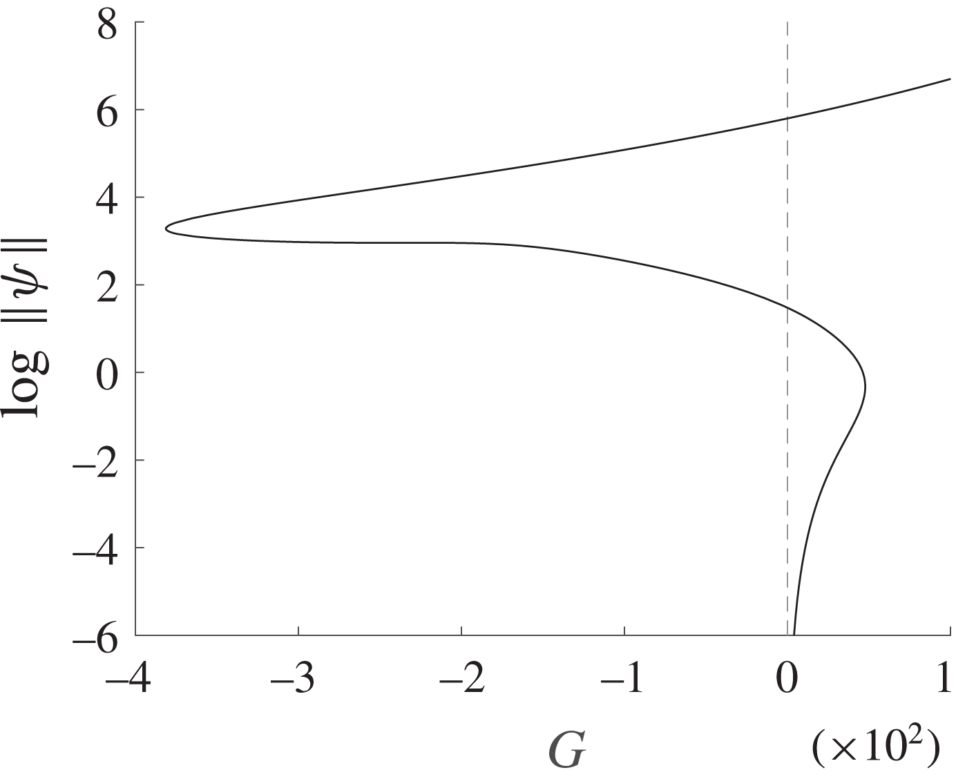
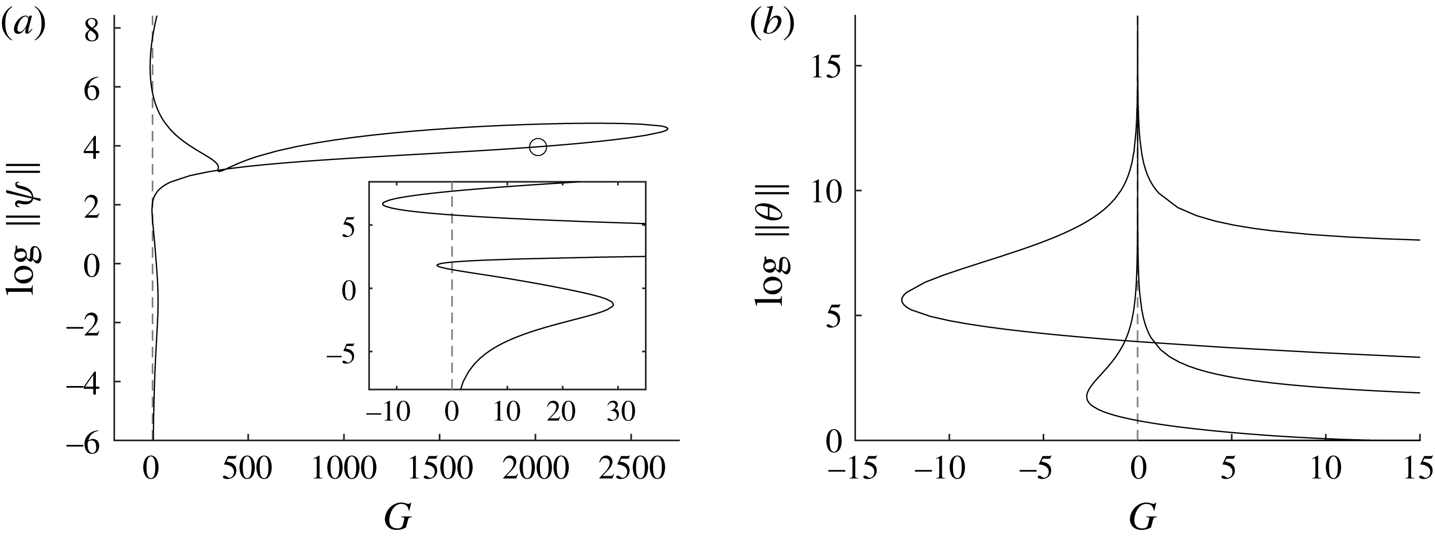
Bifurcation diagrams for $Pr=0.5$ . On (a) we have the logarithm of $\Vert \unicode[STIX]{x1D713}\Vert$ as a function of $G$ , and we observe four distinct solutions with $G=0$ . In the interest of clarity, the region near $G=0$ has been magnified to display all relevant behaviour. We have marked with a circle the point for which we show the solution profiles in figure 6. On (b) we have the logarithm of $\Vert \unicode[STIX]{x1D703}\Vert$ , and observe that two of the solutions with $G=0$ have finite $\unicode[STIX]{x1D703}$ , and in the other two we have $\unicode[STIX]{x1D703}\sim 1/G$ as $G\rightarrow 0$ .

Figure 6.

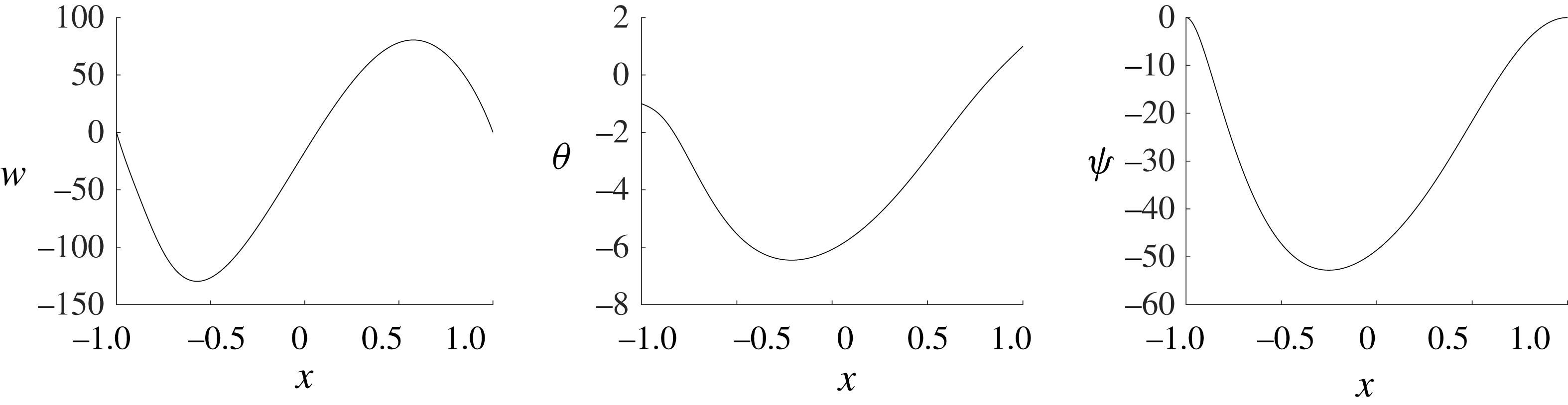
Velocity and temperature profiles for $Pr=0.5$ and $G=2.02\times 10^{3}$ . We see $w<0$ close to the inner wall which has imposed $\unicode[STIX]{x1D703}=-1$ , whereas $w>0$ near the outer ( $\unicode[STIX]{x1D703}=1$ ) wall. The $x$ -velocity is towards the inner wall, as $\unicode[STIX]{x1D713}<0$ . Note that the temperature is not bounded by the boundary conditions, $|\unicode[STIX]{x1D703}|>1$ .

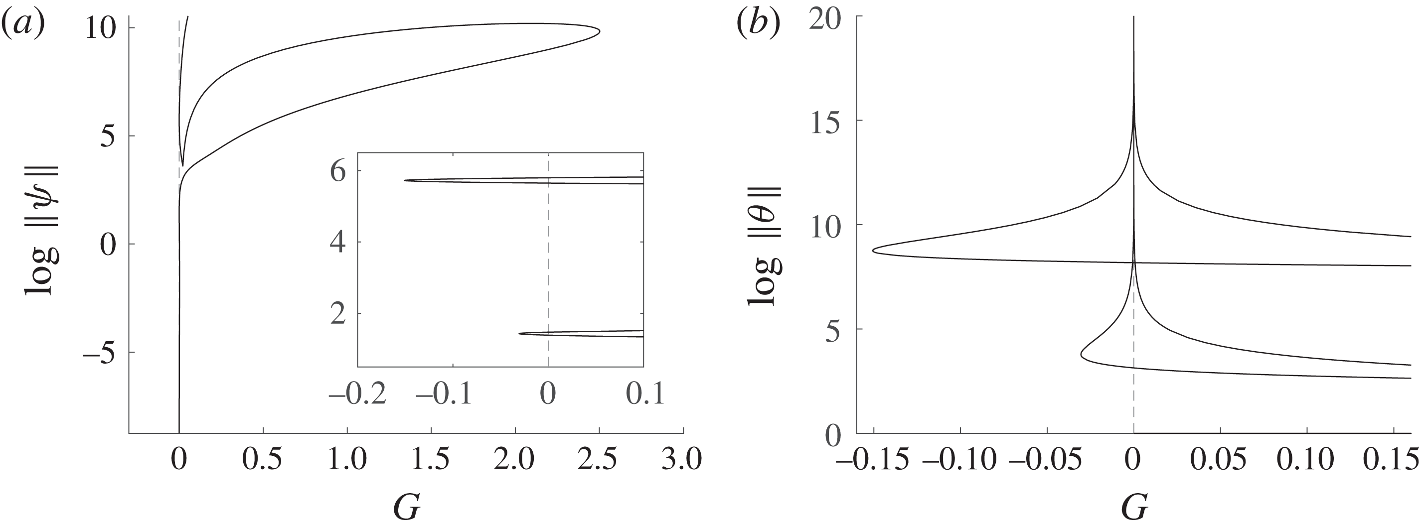
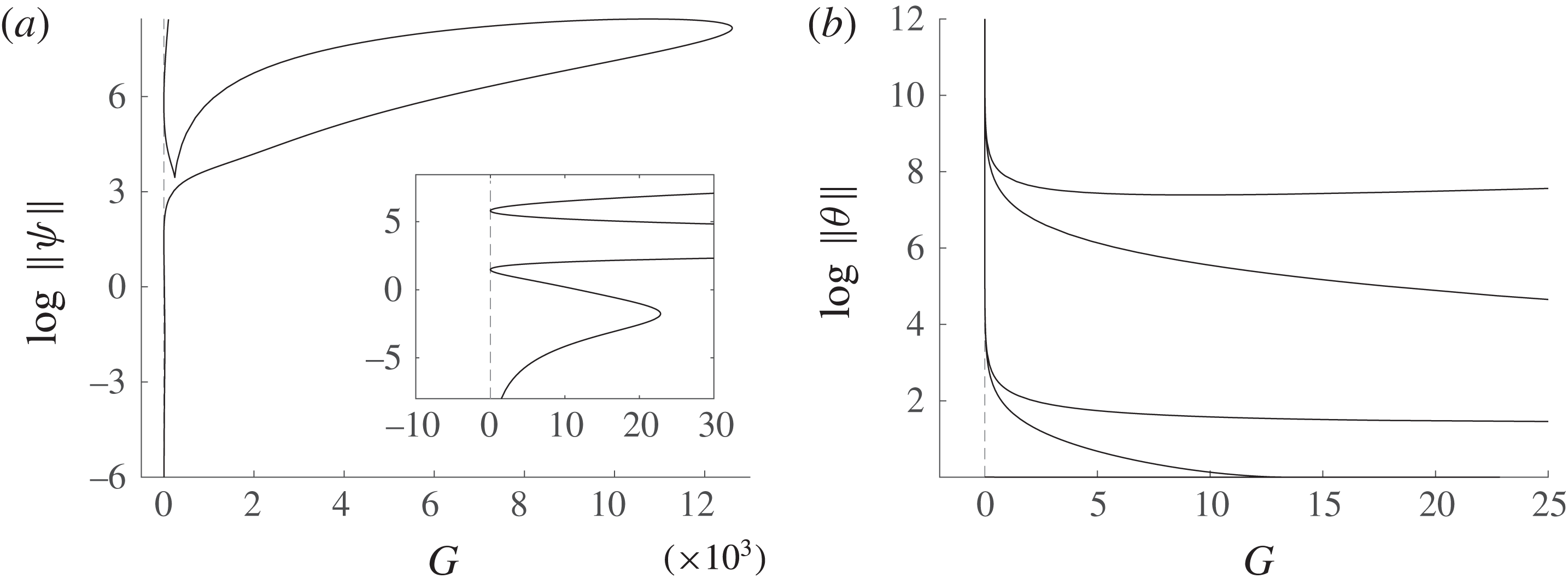
The solution is found to be multivalued in all cases studied, and exhibits four solutions at $G=0$ for every $Pr$ value considered, except for the two special cases $Pr=1$ and $Pr=0$ discussed below. The bifurcation diagrams are shown for $Pr=0.5$ , in figure 5, and for $Pr=1.1$ , in figure 7. As we consider different measures from the ones in the previous section the $\unicode[STIX]{x1D713}$ diagram for $Pr=0.5$ differs from figure 4, but the turning points occur at the same values of $G$ .

For $Pr=0.5$ , in figure 6, we show the velocity and temperature profiles of the point marked in figure 5 with $G=2.02\times 10^{3}$ . The velocity and temperature profiles exhibit the same key characteristics that we found for moderate $G$ , before the first turning point (figure 2), except for the temperature profile that is no longer approximately linear. This implies that the nonlinear terms in (2.13) become important, which we expect since the magnitude of $\unicode[STIX]{x1D713}$ has increased several orders. In addition, the temperature is not bounded by the boundary conditions, $|\unicode[STIX]{x1D703}|>1$ , but is still of the same order.

Figure 7.

Bifurcation diagrams for $Pr=1.1$ . On (a) we have the logarithm of $\Vert \unicode[STIX]{x1D713}\Vert$ as a function of $G$ , and we observe four distinct solutions with $G=0$ . In the interest of clarity, the region near $G=0$ has been magnified to display all relevant behaviour. On (b) we have the logarithm of $\Vert \unicode[STIX]{x1D703}\Vert$ , and again we can observe four unforced solutions, where in two of those cases $\unicode[STIX]{x1D703}\sim 1/G$ as $G\rightarrow 0$ .

We identify two types of unforced solutions. In the first case the temperature fully decouples from the problem and we refer to these as hydrodynamic unforced solutions. We may think of these as zero gravity solutions, with non-zero flow and a passive temperature field. In the second case $\unicode[STIX]{x1D703}\sim 1/G$ as $G\rightarrow 0$ , so that the buoyancy term remains in (2.11). We refer to these as thermally induced. It would of course be physically questionable were the actual temperature to become infinite, as say the Boussinesq approximation would break down. However, if the wall temperature difference $\unicode[STIX]{x0394}T\rightarrow 0$ , it is quite consistent for the temperature, $T$ and the buoyancy term to remain $O(1)$ even though $\unicode[STIX]{x1D703}$ is formally infinite. Following this solution branch through $G=0$ leads to other physical solution branches. In this case, as $|\unicode[STIX]{x1D703}|\gg 1$ , the solution with the boundary conditions $\unicode[STIX]{x1D703}(\pm 1)=\pm 1$ is a small perturbation of an unforced solution with $\unicode[STIX]{x1D703}(\pm 1)=0$ . The existence of both kinds of unforced solutions can be explained by the unbounded nature of the domain which permits advection from $y=\pm \infty$ . Nevertheless, their existence has not been previously reported.

Figure 8.

Bifurcation diagrams for $Pr=1$ . On (a) we have the logarithm of $\Vert \unicode[STIX]{x1D713}\Vert$ as a function of $G$ , and we observe two solutions with $G=0$ . On (b) we have the logarithm of $\Vert \unicode[STIX]{x1D703}\Vert$ , and we observe that both solutions at $G=0$ are singular for $Pr=1$ each pair of thermal and hydrodynamic unforced solutions merges into one solution. Despite the temperature being singular we have $\unicode[STIX]{x1D703}\sim G^{-1/2}$ as $G\rightarrow 0$ , thus the velocity field remains unaffected by temperature.

In the case $Pr=1$ we observe only two unforced flows, shown in figure 8. These must be the unforced hydrodynamic flows, which exist independently of $Pr$ . The scaled temperature field is formally infinite as $G\rightarrow 0$ , but does not modify the flow. This can be explained as follows. Regarding $\unicode[STIX]{x1D713}$ as given, we can rewrite (2.11) and (2.12) in the self-adjoint Sturm–Liouville form,

(5.2) $$\begin{eqnarray}\displaystyle & \displaystyle (pw^{\prime })^{\prime }+qw=-Gp\unicode[STIX]{x1D703}, & \displaystyle\end{eqnarray}$$

(5.3) $$\begin{eqnarray}\displaystyle & \displaystyle (p\unicode[STIX]{x1D703}^{\prime })^{\prime }+q\unicode[STIX]{x1D703}=0, & \displaystyle\end{eqnarray}$$

where

(5.4a,b ) $$\begin{eqnarray}p^{\prime }=-p\unicode[STIX]{x1D713},\quad q=p\unicode[STIX]{x1D713}^{\prime }.\end{eqnarray}$$

Multiplying (5.2) by $\unicode[STIX]{x1D703}$ and (5.3) by $w$ , subtracting and integrating between $x=\pm 1$ , we obtain

(5.5) $$\begin{eqnarray}-\int _{-1}^{1}Gp\unicode[STIX]{x1D703}^{2}\,\text{d}x=[pw^{\prime }\unicode[STIX]{x1D703}-pw\unicode[STIX]{x1D703}^{\prime }]_{-1}^{1}.\end{eqnarray}$$

Imposing the boundary conditions we obtain

(5.6) $$\begin{eqnarray}p(1)w^{\prime }(1)+p(-1)w^{\prime }(-1)=-\int _{-1}^{1}Gp\unicode[STIX]{x1D703}^{2}\,\text{d}x.\end{eqnarray}$$

There is no reason why the left-hand side should vanish (for example if $w$ is odd it cannot). As $G\rightarrow 0$ , we infer that $\unicode[STIX]{x1D703}\propto G^{-1/2}$ . It follows that the $G\unicode[STIX]{x1D703}$ term becomes negligible, and the associated flow approaches the unforced hydrodynamic flow. This behaviour is confirmed numerically.

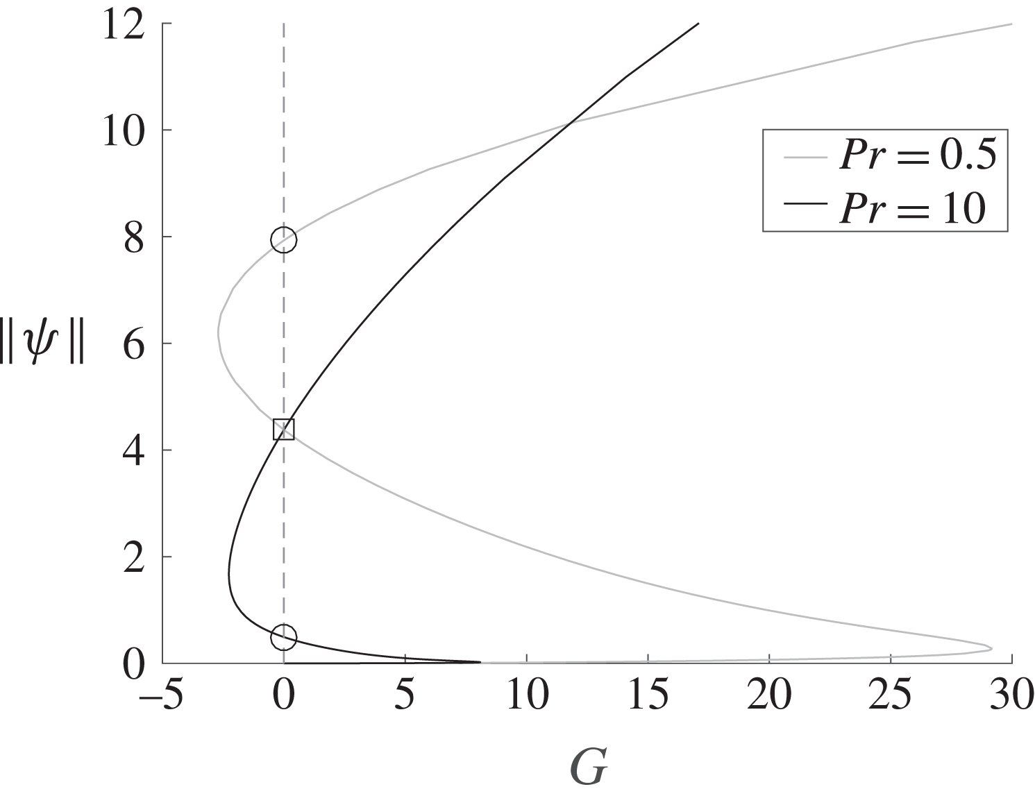
Another characteristic of the system is that as $Pr$ passes through $1$ , the hydrodynamic unforced solutions and the thermally induced ones swap their order of appearance. In order to illustrate this, we show in figure 9, the bifurcation diagram for $Pr=0.5$ and $10$ , for the first unforced hydrodynamic solution and the first thermally induced one.

Figure 9.

Bifurcation diagrams for $Pr=0.5$ and $10$ . Illustration of the change in order of appearance of the hydrodynamic solution (marked with squares) and the thermally induced one (marked with circles). This swap occurs at $Pr=1$ .

The other special case is the limit $Pr\rightarrow 0$ , when (2.13) reduces to $\unicode[STIX]{x1D703}^{\prime \prime }=0$ , with the linear solution, $\unicode[STIX]{x1D703}(x)=x$ . Therefore, in this case solutions with $\unicode[STIX]{x1D703}\sim 1/G$ are not possible. Indeed, the only unforced solutions we find decouple from $\unicode[STIX]{x1D703}$ . Figure 10, shows the bifurcation diagram for $Pr=0$ .

Figure 10.

Bifurcation diagram for $Pr=0$ , showing $\log \Vert \unicode[STIX]{x1D713}\Vert$ as a function of $G$ . There are two fully hydrodynamic solutions for $G=0$ .

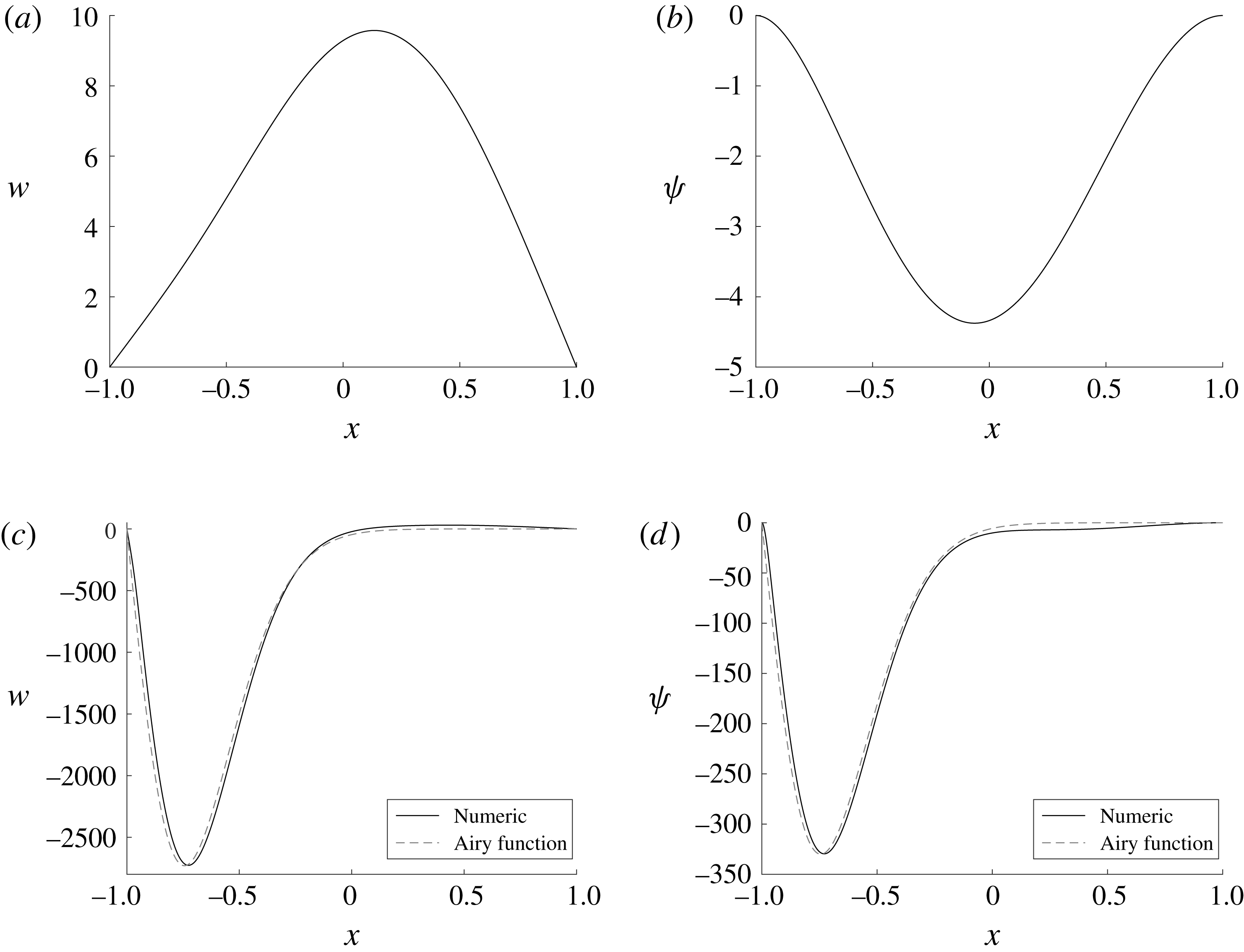
The fully hydrodynamic unforced solutions are naturally independent of the $Pr$ number. The $w$ and $\unicode[STIX]{x1D713}$ profiles are presented in figure 11. In the top solution all variables are $O(1)$ and there are no small length scales. In the lower solution however, the flow is large in magnitude, suggesting that it is inertially dominated. If the viscous terms in (2.11) and (2.12) are neglected, then the equations have the general solution for arbitrary constants $A$ , $C$ , $x_{0}$

(5.7a,b ) $$\begin{eqnarray}w=A\unicode[STIX]{x1D713},\quad \unicode[STIX]{x1D713}=C\text{Ai}[(2A^{2})^{1/3}(x-x_{0})],\end{eqnarray}$$

where Ai is an Airy function. The constant $x_{0}$ can be chosen to satisfy the solid wall condition $\unicode[STIX]{x1D713}(-1)=0$ . The no-slip condition at the inner wall requires a viscous layer of thickness $O(C^{-1/2})$ . Note that matching with the core requires that $C<0$ , so that the core flow is directed towards the viscous stagnation point. For $x\gg x_{0}$ , the Airy function decays exponentially and the viscous terms become important before the outer wall is reached. It is worth observing that although asymptotic matching is useful here, strictly speaking $C$ has a fixed finite value rather than being arbitrarily large. Nevertheless, as shown in the figure, there is good agreement between the numerical solution and the Airy approximation.

Figure 11.

$\unicode[STIX]{x1D713}$ and $w$ profiles for fully hydrodynamic unforced solutions. (a,b) First hydrodynamic unforced solution. (c,d) Second hydrodynamic unforced solution, with inviscid core and boundary layer on inner wall. There is good agreement between the numerical solution and the Airy function, equation (5.7).

We have not yet remarked on the stability of our solutions. We can obtain some information in a fairly straightforward manner by computing the eigenvalues of the Jacobian of our discretised system, equation (5.1) (Sharma et al. Reference Sharma, Coetzee, Lowenberg, Neild and Krauskopf2015). This analysis indicates that the lower solution branch is stable, but after the first turning point the solution branches are unstable. We should stress that these conclusions only address temporal stability to modes of the same spatial structure as the solution.

Our main focus so far has been on the study of steady state solutions and we have not considered what happens for large $G$ . For example, for $Pr=0.5$ we have not found any solution for $G\gtrsim 2.7\times 10^{3}$ . Numerical solution of the time dependent equations,

(5.8) $$\begin{eqnarray}\displaystyle & \displaystyle \frac{\unicode[STIX]{x2202}w}{\unicode[STIX]{x2202}t}+w^{\prime }\unicode[STIX]{x1D713}-w\unicode[STIX]{x1D713}^{\prime }=w^{\prime \prime }+G\unicode[STIX]{x1D703}, & \displaystyle\end{eqnarray}$$

(5.9) $$\begin{eqnarray}\displaystyle & \displaystyle \frac{\unicode[STIX]{x2202}\unicode[STIX]{x1D713}^{\prime \prime }}{\unicode[STIX]{x2202}t}+\unicode[STIX]{x1D713}^{\prime \prime \prime }\unicode[STIX]{x1D713}-\unicode[STIX]{x1D713}^{\prime \prime }\unicode[STIX]{x1D713}^{\prime }=\unicode[STIX]{x1D713}^{\prime \prime \prime \prime }+2w^{2}, & \displaystyle\end{eqnarray}$$

(5.10) $$\begin{eqnarray}\displaystyle & \displaystyle \frac{\unicode[STIX]{x2202}\unicode[STIX]{x1D703}}{\unicode[STIX]{x2202}t}+\unicode[STIX]{x1D703}^{\prime }\unicode[STIX]{x1D713}-\unicode[STIX]{x1D703}\unicode[STIX]{x1D713}^{\prime }=Pr^{-1}\unicode[STIX]{x1D703}^{\prime \prime }, & \displaystyle\end{eqnarray}$$

indicates that this system becomes singular in finite time. This is reminiscent of the work of Childress et al. (Reference Childress, Ierley, Spiegel and Young1989). We find that near some critical time $t_{0}$ , away from the walls our variables behave as

(5.11a-c ) $$\begin{eqnarray}w(x,t)\sim \frac{f(x)}{t_{0}-t},\quad \unicode[STIX]{x1D713}(x,t)\sim \frac{g(x)}{t_{0}-t},\quad \unicode[STIX]{x1D703}(x,t)\sim \frac{h(x)}{t_{0}-t}.\end{eqnarray}$$

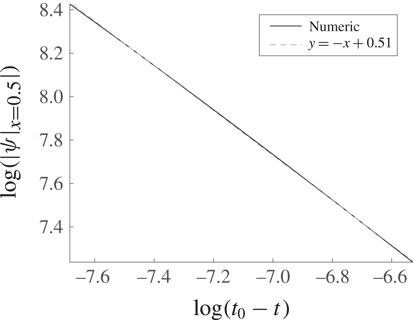
The buoyancy and diffusive terms become negligible away from the walls as they behave as $(t_{0}-t)^{-1}$ rather than $(t_{0}-t)^{-2}$ . There are boundary layers near the walls of thickness $(t_{0}-t)^{1/2}.$ As an example, we set $Pr=0.5$ , for which the stable steady state ceases for $G\geqslant 29.1$ . If we follow the time evolution of a zero initial state for $G=60$ , we find that the solution becomes singular at $t_{0}\simeq 2.55$ . We illustrate this case in figure 12, where the $(t_{0}-t)^{-1}$ behaviour is demonstrated by linear fitting.

Figure 12.

$\log (|\unicode[STIX]{x1D713}|_{x=0.5}|)$ as a function of $\log (t_{0}-t)$ near time singularity for $Pr=0.5$ and $G=60$ . Evolution from a zero initial state. The solution becomes singular at $t_{0}\simeq 2.55$ . The behaviour $(t_{0}-t)^{-1}$ is evident (dashed grey line).

For any value of $Pr$ , as the solution branches are followed, eventually the velocity becomes large, resulting in a wall boundary layer. Adequate resolution requires a high number of mesh points which in turn leads to conditioning issues for the Jacobian matrix. Away from the walls the flow is inertially dominated, unaffected by the temperature similar to (5.7). For the rest of the paper we therefore focus attention on the unforced hydrodynamic solutions. In order to ascertain whether these are generic to the NS, rather than an artifice of the Dean approximation, in the next section we relax the assumption of small curvature so that our infinite channel transforms into the gap between two concentric cylinders. This annular geometry can then support any value of curvature.

Figure 13.

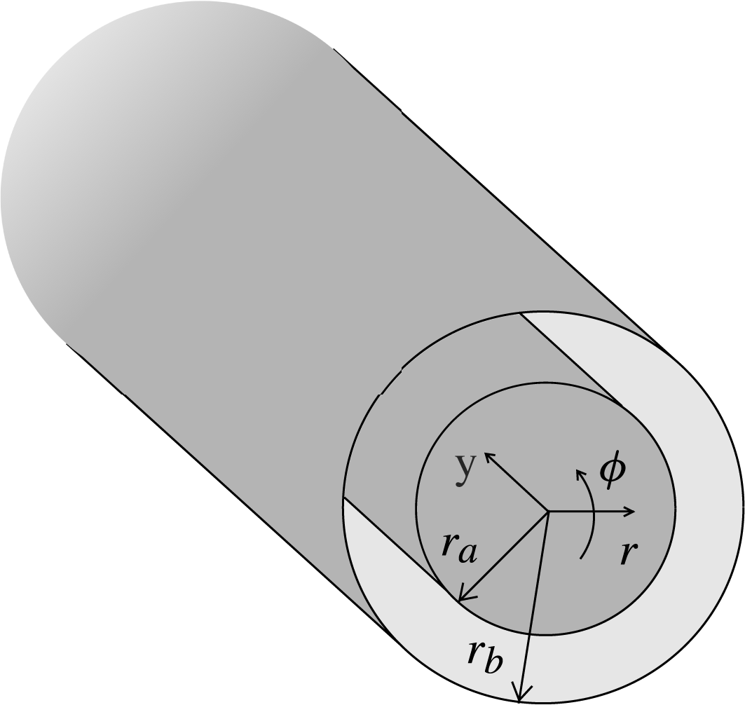
Depiction of annulus geometry and coordinate system $(r,\unicode[STIX]{x1D719},y)$ . The annulus is unbounded in the $y$ direction.

6 Unforced flow in an infinite annulus

We consider steady and axisymmetric flow inside an annulus. The coordinate system is $(r,\unicode[STIX]{x1D719},y)$ , and the inner and outer radii are given by $r_{a}$ and $r_{b}$ , respectively, as drawn in figure 13. We introduce a Stokes streamfunction, $y\unicode[STIX]{x1D713}(r)$ , and the velocity field is described by,

(6.1) $$\begin{eqnarray}\boldsymbol{u}=\left(-\frac{\unicode[STIX]{x1D713}}{r},yw,y\frac{\unicode[STIX]{x1D713}^{\prime }}{r}\right).\end{eqnarray}$$

In addition we scale $w$ and $\unicode[STIX]{x1D713}$ with the Reynolds number. Thus, the NS equations reduce to:

(6.2) $$\begin{eqnarray}\displaystyle & \displaystyle -\unicode[STIX]{x1D713}w^{\prime }+\unicode[STIX]{x1D713}^{\prime }w-\frac{\unicode[STIX]{x1D713}w}{r}=w^{\prime \prime }r+w^{\prime }-\frac{w}{r}, & \displaystyle\end{eqnarray}$$

(6.3) $$\begin{eqnarray}\displaystyle & \displaystyle \qquad -\unicode[STIX]{x1D713}^{\prime \prime \prime }\unicode[STIX]{x1D713}+\unicode[STIX]{x1D713}^{\prime \prime }\unicode[STIX]{x1D713}^{\prime }+3\frac{\unicode[STIX]{x1D713}^{\prime \prime }\unicode[STIX]{x1D713}}{r}-\frac{(\unicode[STIX]{x1D713}^{\prime })^{2}}{r}-3\frac{\unicode[STIX]{x1D713}^{\prime }\unicode[STIX]{x1D713}}{r^{2}}+2w^{2}r & \displaystyle \nonumber\\ \displaystyle & \displaystyle \qquad \qquad \qquad \qquad ~=\unicode[STIX]{x1D713}^{\prime \prime \prime \prime }r-2\unicode[STIX]{x1D713}^{\prime \prime \prime }+3\frac{\unicode[STIX]{x1D713}^{\prime \prime }}{r}-3\frac{\unicode[STIX]{x1D713}^{\prime }}{r^{2}}+F, & \displaystyle\end{eqnarray}$$

where $F$ is a fictitious forcing which we use as a continuation parameter. We seek non-trivial solutions with $F=0$ . We impose no-slip boundary conditions at the wall,

(6.4) $$\begin{eqnarray}w(r_{a,b})=\unicode[STIX]{x1D713}(r_{a,b})=\unicode[STIX]{x1D713}^{\prime }(r_{a,b})=0.\end{eqnarray}$$

The curvature is given by,

(6.5) $$\begin{eqnarray}\unicode[STIX]{x1D706}=\frac{2(r_{b}-r_{a})}{r_{b}+r_{a}},\end{eqnarray}$$

which has the maximum value of $\unicode[STIX]{x1D706}=2$ , that occurs in the limit $r_{b}\gg r_{a}$ . In order to reduce the number of parameters in our problem we have fixed the gap width to $r_{b}-r_{a}=2$ , the same as the channel.

We use second-order centred finite differences to discretise our equations and the path-continuation techniques described in the previous section. We use the two fully hydrodynamic solutions obtained with the Dean equations as initial estimates for small $\unicode[STIX]{x1D706}$ . Once we obtain a converged solution, we perform continuation in $\unicode[STIX]{x1D706}$ to find the solutions for larger curvatures where we observe a more intricate structure as $\unicode[STIX]{x1D706}\rightarrow 2$ . 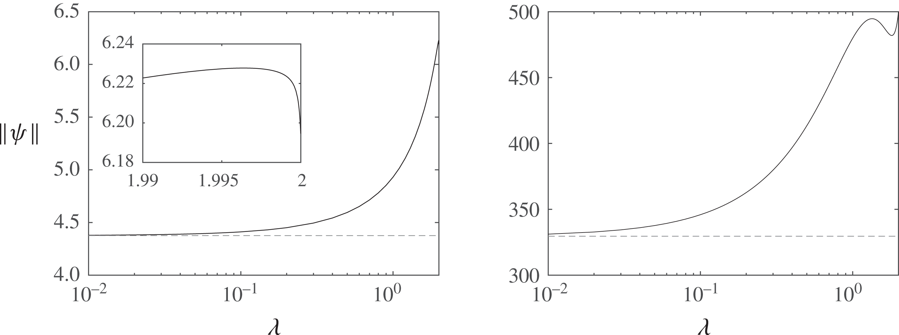In figure 14, we show $\Vert \unicode[STIX]{x1D713}\Vert$ as a function of $\unicode[STIX]{x1D706}$ . As expected, for small curvature values the solutions tend to the Dean solutions, indicated by a dashed line in figure 14.

Figure 14.

Dependence of $\Vert \unicode[STIX]{x1D713}\Vert$ with $\unicode[STIX]{x1D706}$ , for the two hydrodynamic unforced solutions. The dashed grey lines mark the solutions obtained with the Dean equations, which we retrieve when $\unicode[STIX]{x1D706}\rightarrow 0$ . We can also observe a different structure as $\unicode[STIX]{x1D706}\rightarrow 2$ . The results with $w$ are similar.

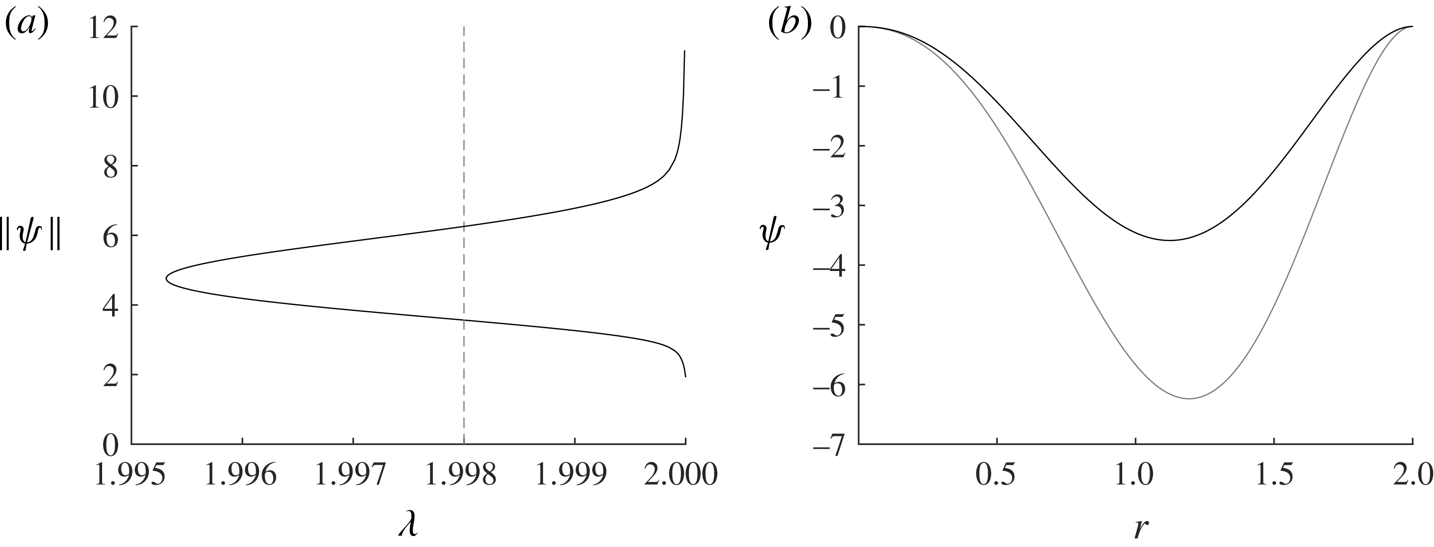
We also look for unforced solutions for the $\unicode[STIX]{x1D713}$ equation decoupled from $w$ , i.e. $w=0$ . In this case, we find that for $\unicode[STIX]{x1D706}\approx 2$ , with $r_{a}/r_{b}\rightarrow 0$ , two $\unicode[STIX]{x1D713}$ -only solutions exist. In figure 15 we can observe $\Vert \unicode[STIX]{x1D713}\Vert$ as a function of $\unicode[STIX]{x1D706}$ , as well as the $\unicode[STIX]{x1D713}$ profiles for $\unicode[STIX]{x1D706}=1.998$ . These solutions only exist for $r_{b}\gg r_{a}$ . We find that along the upper branch, the solution has $\unicode[STIX]{x1D713}\rightarrow \infty$ as $\unicode[STIX]{x1D706}\rightarrow 2$ .

Figure 15.

Solutions of the unforced $\unicode[STIX]{x1D713}$ equation near the maximum value of $\unicode[STIX]{x1D706}$ . For $\unicode[STIX]{x1D706}=1.998$ (highlighted by the dashed grey line), we can observe the $\unicode[STIX]{x1D713}$ profiles for the two solutions found, on (b). These solutions have $w=0$ .

We can rewrite (6.3), in a more compact form, if we consider the variable transformation $\unicode[STIX]{x1D709}=r^{2}$ (Yuan & Finkelstein Reference Yuan and Finkelstein1956),

(6.6) $$\begin{eqnarray}\unicode[STIX]{x1D713}^{\prime }\unicode[STIX]{x1D713}^{\prime \prime }-\unicode[STIX]{x1D713}^{\prime \prime \prime }\unicode[STIX]{x1D713}-4\unicode[STIX]{x1D713}^{\prime \prime \prime }=2\unicode[STIX]{x1D709}\unicode[STIX]{x1D713}^{\prime \prime \prime \prime }+\hat{F},\end{eqnarray}$$

where $\hat{F}$ is a continuation parameter and $^{\prime }$ now denotes a $\unicode[STIX]{x1D709}$ -derivative. The boundary conditions in this case are

(6.7) $$\begin{eqnarray}\unicode[STIX]{x1D713}(r_{a,b}^{2})=\unicode[STIX]{x1D713}^{\prime }(r_{a,b}^{2})=0.\end{eqnarray}$$

We have constructed a power series in $\hat{F}$ , and performed analytical continuation with high-order Hermite–Padé approximants, which confirmed the existence of the two newly found solutions with $\hat{F}=0$ .

7 Summary and concluding remarks

Horizontal temperature gradients always drive motion. For the idealised case of two vertical walls at constant temperature, the flow is one-dimensional. With our two generalisations, including channel curvature and $y$ -variation, the equilibrium flow is three-dimensional and is governed by nonlinear ODEs. The solutions have interesting structure, with multiple solutions even as $G\rightarrow 0$ .

Some of the solutions may be considered ‘local’, in the sense that for given $y$ the temperature lies between the boundary values $\unicode[STIX]{x1D703}=\pm y$ . But in others, including those as $G\rightarrow 0$ , the local temperature is relatively large, suggesting that advection of heat from large $|y|$ is important. This is physically plausible. As the temperature is unbounded as $y\rightarrow \pm \infty$ , it is always possible that advection from infinity should dominate over the local boundary conditions. When this occurs, the solutions are perturbations of what would be obtained with the homogeneous conditions $\unicode[STIX]{x1D703}(\pm 1)=0$ . We call such solutions ‘unforced’. We have distinguished two types of unforced solutions for $G=0$ , hydrodynamic and thermal. In the first case the temperature fully decouples from the hydrodynamics, while in the latter, $\unicode[STIX]{x1D703}$ becomes singular, $\unicode[STIX]{x1D703}\sim 1/G$ as $G\rightarrow 0$ so that the buoyancy forcing remains significant. If we regard $G\rightarrow 0$ as $\unicode[STIX]{x0394}T\rightarrow 0$ , then we note that the physical temperature $T$ remains finite in this limit.

We have presented here results only for moderate Prandtl number. At high $Pr$ the structure of the unforced solutions is similar, while the first critical $G$ value is reduced. The behaviour of the subsequent turning points is, however, more involved.

Stability information can be obtained from the eigenvalues of the Jacobian of the discretised system. This analysis only considers modes of the same spatial structure as the solution, but nevertheless, it reveals that past the first turning point the solution branches are unstable. In order to ascertain the large $G$ behaviour we study the time dependent system, equations (5.8)–(5.10). We then find that the system exhibits a finite-time singularity.

Relaxing the assumption of small curvature, we have shown that the unforced hydrodynamic solutions extend to previously unreported solutions of the full Navier–Stokes in an annulus. These solutions can also be understood as the local solution being dominated by the counterrotating shear flows at $y=\pm \infty$ . However, the annular configuration also yields two extra unforced solutions with $w=0$ , which are harder to visualise. These only exist at high aspect ratio, when $r_{b}\gg r_{a}$ .

The existence of solutions which do not depend on the local boundary conditions but are dominated by the behaviour at infinity may be important in many instances where we have a shear at large distances proportional to $y$ . For example, in recent work, Vaz, Boshier & Mestel (Reference Vaz, Boshier and Mestel2018) we have demonstrated that when the fluid is electrically conducting, the unforced flows described in this paper are able to drive nonlinear dynamos, which may be significant in astrophysical contexts.