1. Introduction
During the past few decades, there has been a widely growing interest in the study of nonlinear wave propagations in dusty plasmas. The existence of dusty plasmas in several important areas, such as planetary rings, asteroid zones, the lower part of the Earth’s ionosphere and magnetosphere (Goertz Reference Goertz1989), coating of thin films (Selwyn Reference Selwyn1993), plasma crystals (Thomas, Morfill & Dammel Reference Thomas, Morfill and Dammel1994) and cometary tails, has become an interesting and challenging research area. Owing to the presence of different types of dust charged grains in a plasma, many interesting new eigenmodes are observed, for example, dust acoustic mode (Rao, Shukla & Yu Reference Rao, Shukla and Yu1990; El-Labany et al. Reference El-Labany, El-Taibany, El-Bedwehy and El-Fayoumy2011), dust-ion acoustic mode (D’Angelo Reference D’Angelo1990; Kourakis & Shukla Reference Kourakis and Shukla2004), dust lattice mode (Melandso Reference Melandso1996), Shukla–Varma mode (Shukla & Varma Reference Shukla and Varma1993), dust Berstain–Green–Kruskal mode (Tribeche & Zerguini Reference Tribeche and Zerguini2004) and dust drift mode (Shukla, Yu & Bharuthram Reference Shukla, Yu and Bharuthram1991). Rao et al. (Reference Rao, Shukla and Yu1990) studied the existence of dust acoustic waves (DAWs) theoretically in an unmagnetized dusty plasmas. Later Shukla & Silin (Reference Shukla and Silin1992) investigated theoretically the characteristics of dust-ion acoustic waves (DIAWs) in dusty plasma. Experimental and theoretical investigations by many researchers, such as D’Angelo (Reference D’Angelo1995), Barkan, Merlino & D’Angelo (Reference Barkan, Merlino and D’Angelo1995, Reference Barkan, Merlino and D’Angelo1996), Nakamura, Bailing & Shukla (Reference Nakamura, Bailung and Shukla1999) and Duan, Lu & Zhao (Reference Duan, Lu and Zhao2001), confirmed the existence of linear and nonlinear phenomena of both DAWs and DIAWs. A number of investigations have been carried out to study nonlinear wave structures, such as solitons, shock and vortices in dusty plasma by several authors (El-Labany & El-Taibany Reference El-Labany and El-Taibany2004; Verheest, Hellberg & Kourakis Reference Verheest, Hellberg and Kourakis2008) during the past few decades.
In most of the theoretical investigations on dusty plasmas, the dust charge was assumed to be constant. However, this assumption is questionable in different realistic situations. Nejoh (Reference Nejoh1997) studied whether the dust grains have a variable charge due to fragmentation, coalescence, etc. It has been proved that the dust charge variation with parameters such as electrostatic plasma potential, electron and ion densities would influence the collective behaviour of the plasma. Thus, the effect of dust charge variation is of great importance in understanding nonlinear wave propagation in dusty plasmas. Xie, He & Huang (Reference Xie, He and Huang1999) investigated dust acoustic solitary waves in a dusty plasma with variable dust charge. They applied the reductive perturbation method to study the soliton solution. But recently Malfliet & Wieers (Reference Malfliet and Wieers1996) reviewed the studies on solitary waves and observed that the reduction perturbation technique is based on the smallness of the amplitude. So the result obtained by them is valid only for small-amplitude solitary waves. Many investigators (Watanabe & Jiang Reference Watanabe and Jiang1993; Chatterjee & Roychoudhury Reference Chatterjee and Roychoudhury1994; Chatterjee & Das Reference Chatterjee and Das2004b
) studied solitary waves in plasmas through a non-perturbative approach by using Sagdeev’s pseudopotential technique. More recently, Johnston & Epstein (Reference Johnston and Epstein2000) derived Sagdeev’s potential in terms of the ion acoustic speed
 $u$
instead of the electric potential
 ${\it\phi}$
. They found that the oscillatory behaviour of the solitary waves may be destroyed as a result of a very small change in the initial conditions. Maitra & Roychoudhury (Reference Maitra and Roychoudhury2003) studied dust acoustic solitary waves through a non-perturbative approach. Chatterjee (Reference Chatterjee2004) and Chatterjee & Das (Reference Chatterjee and Das2004a
,Reference Chatterjee and Das
b
) studied the effect of different parameters on the critical value of the ion speed
 $u$
of the solitary waves beyond which solitary waves cease to exist. Recently, Tribeche & Bacha (Reference Tribeche and Bacha2010) studied nonlinear DAWs in a charge-varying dusty plasma and obtained some soliton-like solutions for the electrostatic potential. A number of works (Rao & Shukla Reference Rao and Shukla1994; Mendis Reference Mendis2002; Asgari, Muniandy & Wong Reference Asgari, Muniandy and Wong2011) have been reported on DAWs considering dust charge fluctuations. In two of those works (Mendis Reference Mendis2002; Asgari et al.
Reference Asgari, Muniandy and Wong2011), the authors considered the inside ionopause plasma with the following parameters:
 $n_{e}=10^{3}~\text{cm}^{-3}$
,
 $T_{e}=0.1~\text{eV}$
,
 $n_{d}=10^{-3}~\text{cm}^{-3}$
,
 $r_{d}=10^{-6}~\text{cm}$
and
 $z_{d}=10^{3}$
, which gives the numerical value of
 ${\it\omega}/{\it\eta}\approx 10^{-1}$
. It is clear that the DAW frequency
 ${\it\omega}$
and the dust charging frequency
 ${\it\eta}$
are comparable for the inside ionopause plasma. Hence, the DAW time period and the dust charging time period are comparable for the inside ionopause plasma. Thus, the present work is valid for space plasma environments, where the DAW frequency
 ${\it\omega}$
and the dust charging frequency
 ${\it\eta}$
are comparable.
Recently, Samanta, Saha & Chatterjee (Reference Samanta, Saha and Chatterjee2013a ,Reference Samanta, Saha and Chatterjee b ,Reference Samanta, Saha and Chatterjee c ) investigated small-amplitude nonlinear travelling waves in plasmas in the frameworks of the Kadomtsev–Petviashili (KP) equation and the Zakharov–Kuznetsov (ZK) equation obtained by the reductive perturbation technique (RPT) by using the bifurcation theory of planar dynamical systems. Saha & Chatterjee (Reference Saha and Chatterjee2014a ) studied nonlinear electron acoustic travelling waves in an unmagnetized quantum plasma in the framework of the Korteweg–de Vries (KdV) equation obtained by the RPT by using the bifurcation theory of planar dynamical systems. Very recently, Saha & Chatterjee investigated ion acoustic (Saha & Chatterjee Reference Saha and Chatterjee2014b ,Reference Saha and Chatterjee c ) and dust acoustic (Saha & Chatterjee Reference Saha and Chatterjee2014d ,Reference Saha and Chatterjee e ) solitary and periodic waves through a non-perturbative approach.
In the present work, our aim is to study dust acoustic solitary waves, blow-up solitary waves and periodic waves in an unmagnetized dusty plasma with Maxwell-distributed electrons and ions with variable dust charge using the bifurcation theory of planar dynamical systems. Four exact solutions of the solitary, blow-up solitary and periodic waves are derived depending on the physical parameters. Regarding the solitary, blow-up solitary and periodic wave solutions, we have presented the combined effects of the density ratio of electrons and ions (
 ${\it\alpha}$
), temperature ratio of electrons and ions
 $({\it\beta})$
and speed of the travelling wave (
 $v$
).
The remainder of the paper is organized as follows: In § 2, we consider basic equations. In § 3, we obtain bifurcations of phase portraits. Four exact solutions are presented in § 4. We discuss the parametric effects in § 5, and § 6 is kept for conclusions.
2. Basic equations
In this work, we consider a collisionless unmagnetized three-component dusty plasma with dust charge fluctuations. In this case, the plasma contains negatively charged dust particles, Maxwell-distributed electrons and ions. The dynamics of low-phase-velocity nonlinear DAWs is described by the following normalized equations:
 $$\begin{eqnarray}\displaystyle & \displaystyle \frac{\partial n_{d}}{\partial t}+\frac{\partial (n_{d}u_{d})}{\partial x}=0, & \displaystyle\end{eqnarray}$$
 $$\begin{eqnarray}\displaystyle & \displaystyle \frac{\partial u_{d}}{\partial t}+u_{d}\frac{\partial u_{d}}{\partial x}=z_{d}\frac{\partial {\it\phi}}{\partial x}, & \displaystyle\end{eqnarray}$$
 $$\begin{eqnarray}\displaystyle & \displaystyle \frac{\partial ^{2}{\it\phi}}{\partial x^{2}}=(1-{\it\alpha})z_{d}n_{d}+n_{e}-n_{i}, & \displaystyle\end{eqnarray}$$
 $$\begin{eqnarray}\displaystyle & \displaystyle \left(\frac{\partial }{\partial t}+u_{d}\frac{\partial }{\partial x}\right)Q_{d}=I_{e}+I_{i}. & \displaystyle\end{eqnarray}$$
 $$\begin{eqnarray}\displaystyle \displaystyle n_{e} & = & \displaystyle {\it\alpha}\text{e}^{{\it\phi}},\end{eqnarray}$$
 $$\begin{eqnarray}\displaystyle \displaystyle n_{i} & = & \displaystyle \text{e}^{-{\it\beta}{\it\phi}},\end{eqnarray}$$
 ${\it\alpha}=n_{e0}/n_{i0}$
and
 ${\it\beta}=T_{e}/T_{i}$
. Here
 $n_{d}$
,
 $n_{e}$
and
 $n_{i}$
denote the number densities of the dust particles, electrons and ions, respectively;
 $Q_{d}$
and
 $z_{d}$
are dust charge variable and variable charge number of the dust particles, respectively; and
 $u_{d}$
and
 ${\it\phi}$
are the dust fluid velocity and electrostatic potential, respectively, normalized by the dust acoustic speed
 $c=(Z_{d0}T_{e}/m_{d})^{1/2}$
and
 $T_{e}/e$
, where
 $Z_{d}$
is the number of charges residing on the dust grain surface and
 $m_{d}$
is the mass of dust particles. The time
 $t$
and space variable
 $x$
are normalized to the dust plasma period
 ${\it\omega}^{-1}=(m_{d}/4{\rm\pi}n_{d0}Z_{d0}^{2}\text{e}^{2})^{1/2}$
and the Debye length
 ${\it\lambda}=(T_{e}/4{\rm\pi}n_{e0}z_{d0}\text{e}^{2})^{1/2}$
, respectively.
The current balance equation is given by
 $$\begin{eqnarray}I_{e}+I_{i}=0,\end{eqnarray}$$
where
 $I_{e}$
and
 $I_{i}$
are given by the following relations:
 $$\begin{eqnarray}\displaystyle & \displaystyle I_{e}=-e{\rm\pi}r^{2}\sqrt{\left(\frac{8T_{e}}{{\rm\pi}m_{e}}\right)}\,n_{e}\text{e}^{{\it\phi}}, & \displaystyle\end{eqnarray}$$
 $$\begin{eqnarray}\displaystyle & \displaystyle I_{i}=e{\rm\pi}r^{2}\sqrt{\left(\frac{8T_{i}}{{\rm\pi}m_{i}}\right)}\,n_{i}(1-{\it\beta}{\it\phi}). & \displaystyle\end{eqnarray}$$
 $I_{e}+I_{i}=0$
. Thus, we get a relation between the dust charge and the potential approximately given by (neglecting terms of higher order)
 $$\begin{eqnarray}\displaystyle & \displaystyle z_{d}=1+a{\it\phi}+b{\it\phi}^{2},\qquad \text{where} & \displaystyle \nonumber\\ \displaystyle & a=\displaystyle \frac{2({\it\alpha}\sqrt{{\it\mu}{\it\beta}}+{\it\beta})}{({\it\alpha}\sqrt{{\it\mu}{\it\beta}}-1)}\quad \text{and}\quad b=\displaystyle \frac{3}{2}\frac{(4{\it\alpha}\sqrt{{\it\mu}{\it\beta}}-{\it\beta}^{2})}{({\it\alpha}\sqrt{{\it\mu}{\it\beta}}-1)} & \displaystyle\end{eqnarray}$$
with
 ${\it\mu}=m_{i}/m_{e}$
.
In order to study all localized travelling wave solutions, we introduce a new variable
 ${\it\xi}=x-vt,$
where
 $v$
is the velocity of the travelling wave. Using the new variable
 ${\it\xi}$
and the initial conditions
 $u_{d}=0$
,
 $n_{d}=1$
and
 ${\it\phi}=0$
in (2.1) and (2.2), we get
 $$\begin{eqnarray}\displaystyle n_{d}=\frac{v}{\sqrt{v^{2}+2{\it\phi}+a{\it\phi}^{2}+\displaystyle {\textstyle \frac{2}{3}}b{\it\phi}^{3}}}. & & \displaystyle\end{eqnarray}$$
Using (2.5), (2.6), (2.10) and (2.11) in (2.3) and considering the terms of
 ${\it\phi}$
up to second degree, we have
 $$\begin{eqnarray}\displaystyle & \displaystyle \frac{\text{d}^{2}{\it\phi}}{\text{d}{\it\xi}^{2}}=A{\it\phi}+B{\it\phi}^{2},\qquad \text{where} & \displaystyle \nonumber\\ \displaystyle & \displaystyle A={\it\alpha}+{\it\beta}+(1-{\it\alpha})\left(\!a-\frac{1}{v^{2}}\!\right)\quad \text{and}\quad \displaystyle B=\frac{1}{2}({\it\alpha}-{\it\beta}^{2})+(1-{\it\alpha})\left(\!b+\frac{3}{2v^{2}}(1-a)\!\right). & \displaystyle \nonumber\\ \displaystyle & & \displaystyle\end{eqnarray}$$
Xie et al. (Reference Xie, He and Huang1999) studied dust acoustic solitary waves and double layers in a dusty plasma with variable dust charge and two temperature ions. If one can consider travelling wave transformation, then the KdV equation of Xie et al. (Reference Xie, He and Huang1999) can easily be transformed to an equation that will be similar to equation (2.12). Then, one can obtain the corresponding dynamical system and its phase portraits. Using phase plane analysis with
 $ab>0$
(
 $a$
and
 $b$
are coefficients of the nonlinear term and dispersion term in the KdV equation, respectively) in Xie et al. (Reference Xie, He and Huang1999), one can obtain the solitary wave and periodic wave solutions corresponding to homoclinic and periodic orbits in the phase portrait of the corresponding dynamical system. Applying the same analysis with
 $ab<0$
in Xie et al. (Reference Xie, He and Huang1999), one can derive the blow-up solitary wave and periodic wave solutions corresponding to homoclinic orbit and periodic orbits in the phase portrait of the dynamical system. In Xie et al. (Reference Xie, He and Huang1999), the authors obtained compressive and rarefactive solitary waves of the KdV equation but not a periodic wave solution. But, in this case, we have obtained solitary, blow-up solitary and periodic travelling wave solutions using bifurcation theory of planar dynamical systems. So, the extension is important for further study. It is also important to note that applying bifurcation theory of planar dynamical systems, one can obtain not only solitary but also periodic travelling wave solutions, which is an advantage of this method.
Then (2.12) can be expressed as the following dynamical system:
 $$\begin{eqnarray}\left.\begin{array}{@{}c@{}}\displaystyle \frac{\text{d}{\it\phi}}{\text{d}{\it\xi}}=z,\\ \displaystyle \frac{\text{d}z}{\text{d}{\it\xi}}=A{\it\phi}+B{\it\phi}^{2}.\end{array}\right\}\end{eqnarray}$$
The system (2.13) is a planar Hamiltonian system with Hamiltonian function:
 $$\begin{eqnarray}H({\it\phi},z)=\frac{z^{2}}{2}-A\frac{{\it\phi}^{2}}{2}-B\frac{{\it\phi}^{3}}{3}=h,\text{ say}.\end{eqnarray}$$
The system (2.13) is a planar dynamical system with parameters
 ${\it\alpha},{\it\beta},{\it\mu}$
and
 $v$
. It is well known that the phase orbits defined by the vector fields of (2.13) will determine all travelling wave solutions of (2.12). We will investigate the bifurcations of phase portraits of (2.13) in the
 $({\it\phi},z)$
phase plane depending on the physical parameters. A solitary wave solution of (2.12) corresponds to a homoclinic orbit of (2.13). A periodic orbit of (2.13) corresponds to a periodic travelling wave solution of (2.12).
3. Bifurcations of phase portraits of equation (2.13)
In this section, we study all possible phase orbits defined by the vector field (2.13) as the parameters
 ${\it\alpha},{\it\beta},{\it\mu}$
and
 $v$
are varied. When
 $AB\neq 0$
, then the dynamical system (2.13) has two equilibrium points at
 $E_{0}({\it\phi}_{0},0)$
and
 $E_{1}({\it\phi}_{1},0)$
, with
 ${\it\phi}_{0}=0$
and
 ${\it\phi}_{1}=-A/B$
. If
 $M({\it\phi}_{i},0)$
denotes the coefficient matrix of the linearized system of equations (2.13) at an equilibrium point
 $E_{i}({\it\phi}_{i},0)$
, then one can easily obtain
 $$\begin{eqnarray}J=\det M({\it\phi}_{i},0)=-A-2B{\it\phi}_{i}.\end{eqnarray}$$
By the theory of planar dynamical systems (Guckenheimer & Holmes Reference Guckenheimer and Holmes1983; Saha Reference Saha2012), we know that an equilibrium point
 $E_{i}({\it\phi}_{i},0)$
of the planar dynamical system (2.13) is a saddle point when
 $J<0$
and the equilibrium point
 $E_{i}({\it\phi}_{i},0)$
of the planar dynamical system (2.13) is a centre when
 $J>0$
.
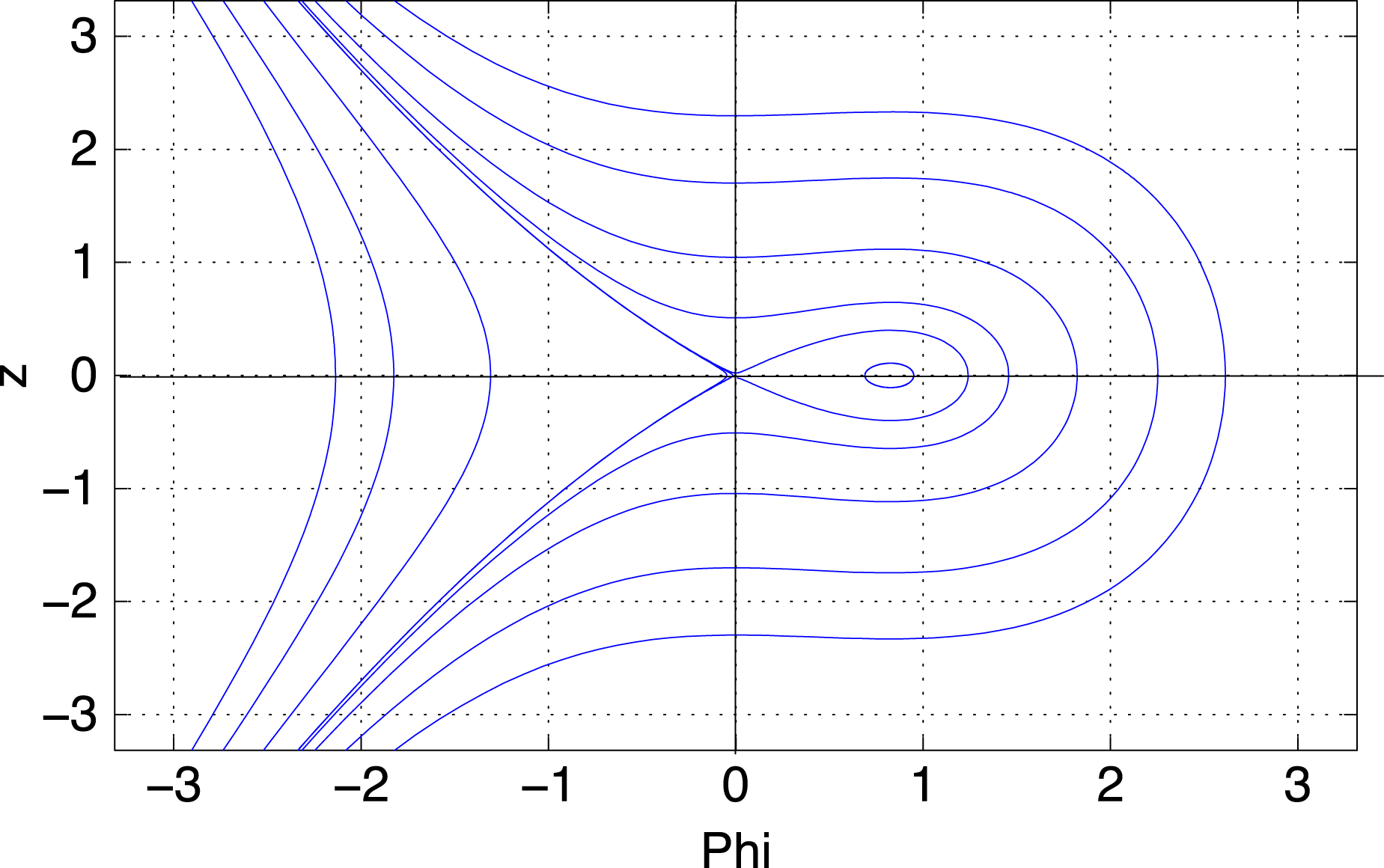
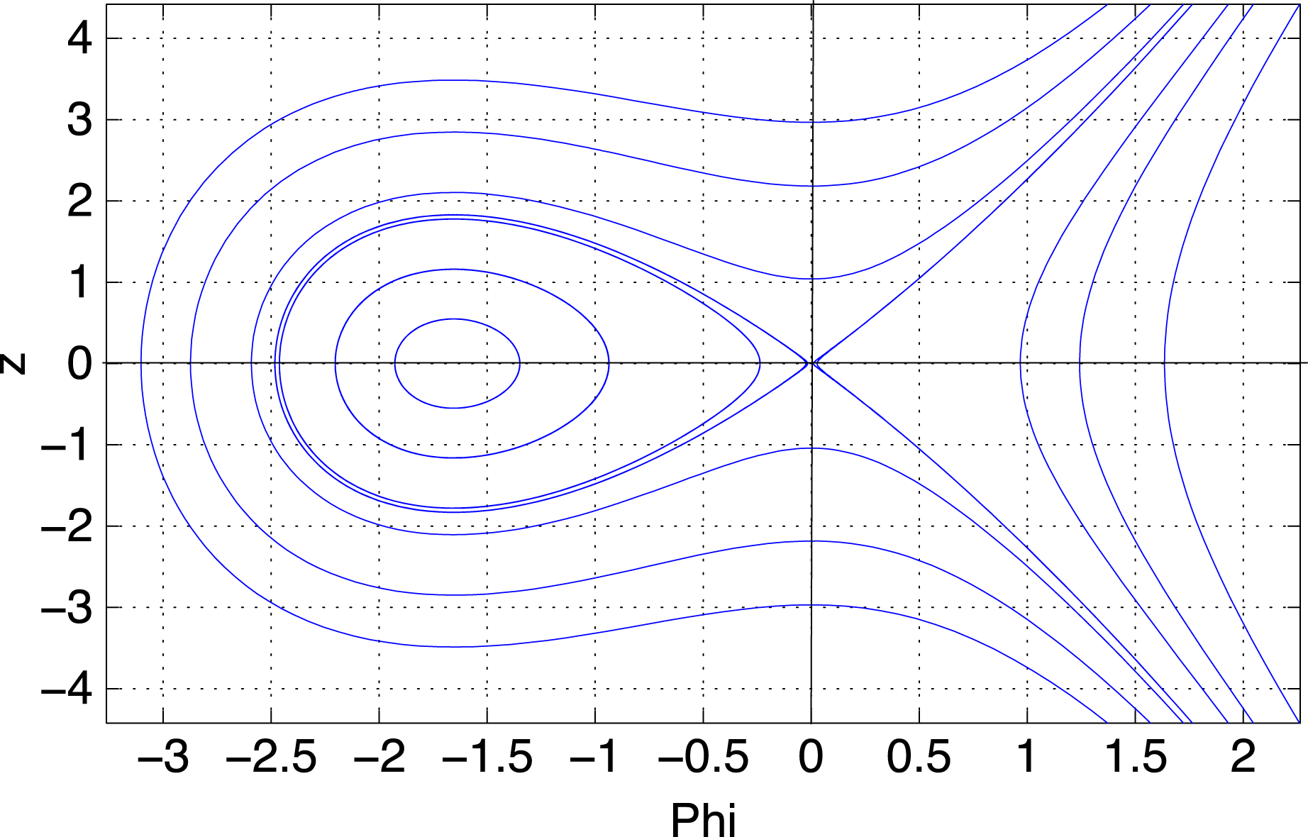
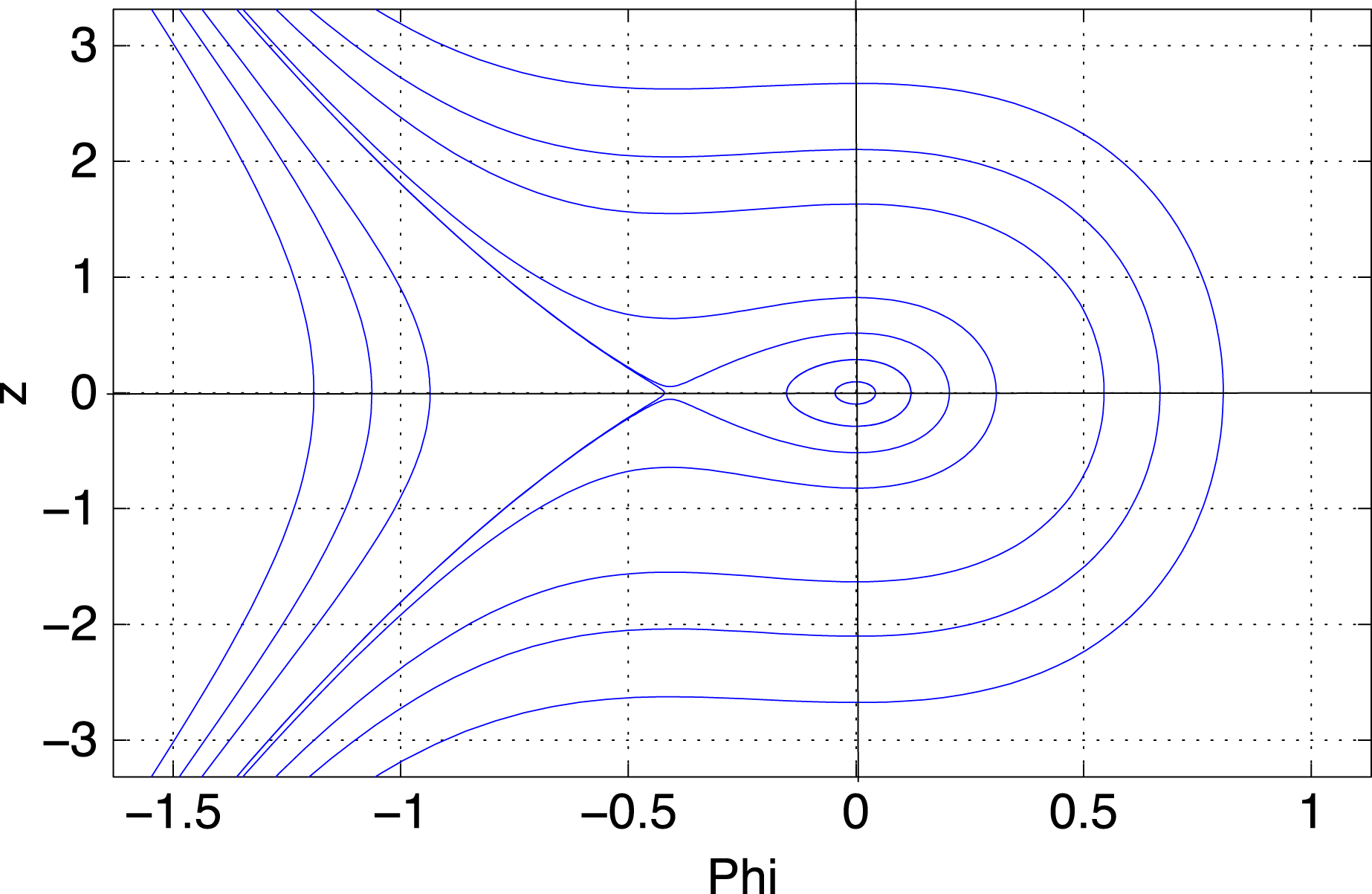
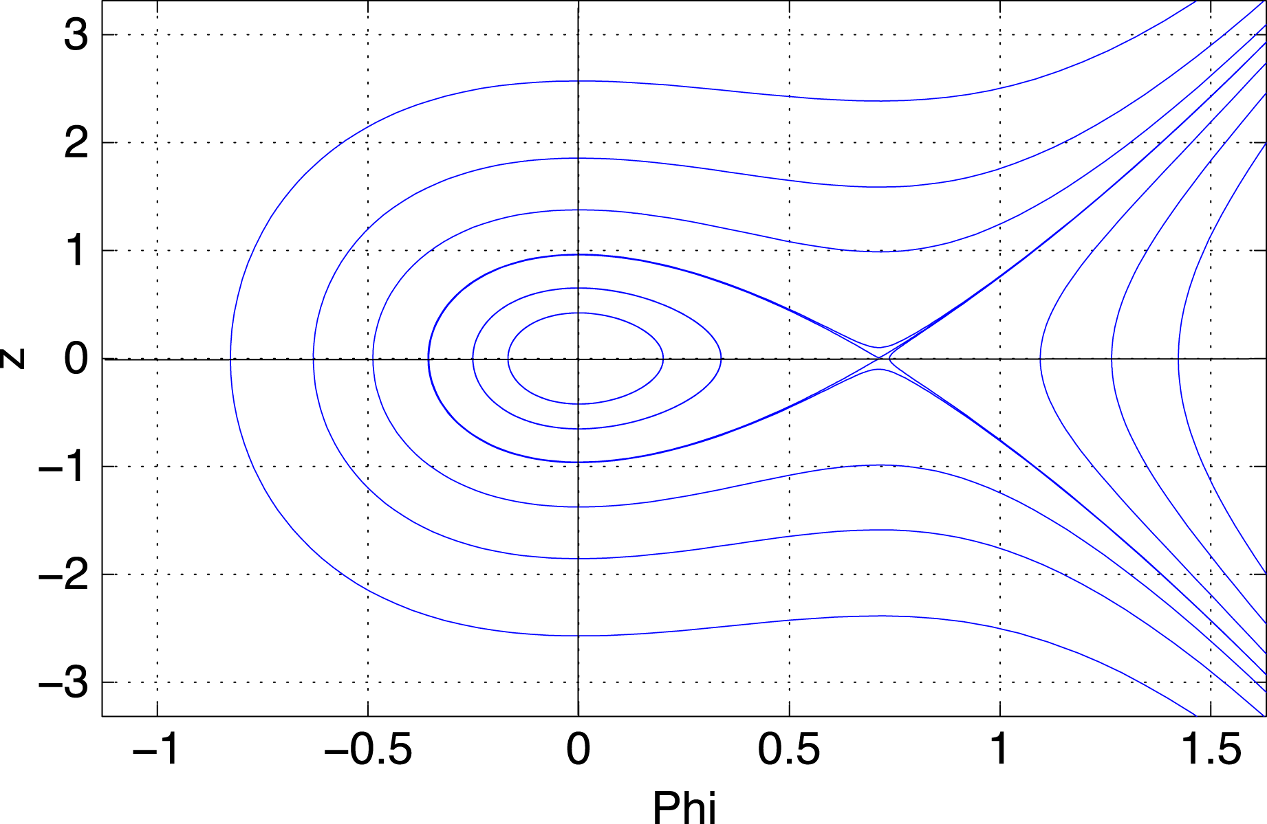
Applying the above analysis, we obtain the different phase portraits of (2.13) depending on the physical parameters
 ${\it\alpha},{\it\beta},{\it\mu}$
and
 $v$
, shown in figures 1–4.
Phase portrait of (2.13) for
 ${\it\alpha}=0.5,{\it\beta}=1.1,{\it\mu}=1837$
and
 $v=0.5$
.

Phase portrait of (2.13) for
 ${\it\alpha}=0.3,{\it\beta}=1.9,{\it\mu}=1837$
and
 $v=2$
.

Phase portrait of (2.13) for
 ${\it\alpha}=0.3,{\it\beta}=1.1,{\it\mu}=1837$
and
 $v=0.3$
.

Phase portrait of (2.13) for
 ${\it\alpha}=0.01,{\it\beta}=1.1,{\it\mu}=1837$
and
 $v=1$
.

For the phase portrait presented in figure 1, the parameters
 ${\it\alpha},{\it\beta},{\it\mu}$
and
 $v$
satisfy the relations
 $A>0$
and
 $B<0$
. In this case the velocity of the travelling wave is subsonic. There exist a homoclinic orbit at the equilibrium point
 $E_{0}({\it\phi}_{0},0)$
and a family of periodic orbits at
 $E_{1}({\it\phi}_{1},0)$
. Here
 $E_{1}({\it\phi}_{1},0)$
is a centre and
 $E_{0}({\it\phi}_{0},0)$
is a saddle point.
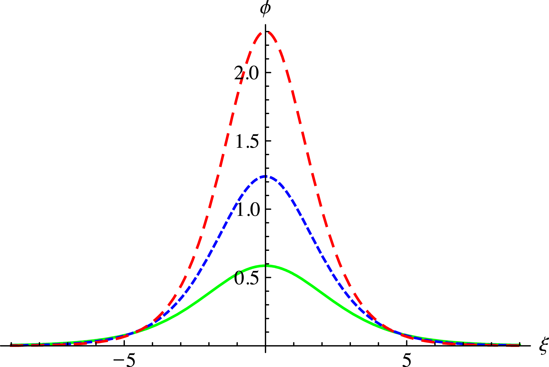
Solitary wave profile of (2.12) plotted for different ratios of electron and ion densities,
 ${\it\alpha}=0.4$
(green full curve),
 ${\it\alpha}=0.5$
(blue dashed curve) and
 ${\it\alpha}=0.6$
(red long dashed curve), with
 ${\it\beta}=1.1,{\it\mu}=1837$
and
 $v=0.5$
.

For the phase portrait presented in figure 2, the parameters
 ${\it\alpha},{\it\beta},{\it\mu}$
and
 $v$
satisfy the relations
 $A>0$
and
 $B>0$
. In this case the velocity of the travelling wave is supersonic. There exist a homoclinic orbit at the equilibrium point
 $E_{0}({\it\phi}_{0},0)$
and a family of periodic orbits at
 $E_{1}({\it\phi}_{1},0)$
. Here
 $E_{1}({\it\phi}_{1},0)$
is a centre and
 $E_{0}({\it\phi}_{0},0)$
is a saddle point.
For the phase portrait presented in figure 3, the parameters
 ${\it\alpha},{\it\beta},{\it\mu}$
and
 $v$
satisfy the relations
 $A<0$
and
 $B<0$
. In this case the velocity of the travelling wave is subsonic. There exist a homoclinic orbit at the equilibrium point
 $E_{1}({\it\phi}_{1},0)$
and a family of periodic orbits at
 $E_{0}({\it\phi}_{0},0)$
. Here
 $E_{1}({\it\phi}_{1},0)$
is a saddle point and
 $E_{0}({\it\phi}_{0},0)$
is a centre.
For the phase portrait presented in figure 4, the parameters
 ${\it\alpha},{\it\beta},{\it\mu}$
and
 $v$
satisfy the relations
 $A<0$
and
 $B>0$
. In this case the velocity of the travelling wave is sonic. There exist a homoclinic orbit at the equilibrium point
 $E_{1}({\it\phi}_{1},0)$
and a family of periodic orbits at
 $E_{0}({\it\phi}_{0},0)$
. Here
 $E_{1}({\it\phi}_{1},0)$
is a saddle point and
 $E_{0}({\it\phi}_{0},0)$
is a centre.
4. Exact solutions of equation (2.12)
In this section, with the help of the planar dynamical system (2.13) and the Hamiltonian function given by (2.14) with
 $h=0$
, we derive dust acoustic solitary wave, blow-up solitary wave and periodic travelling wave solutions of (2.12) depending on different parametric conditions.
-
(i) When
 $A>0$
and
$B<0$
(see figures 1 and 5–7), the system (2.12) has a compressive solitary wave solution given by (4.1)
$$\begin{eqnarray}{\it\phi}=-\frac{3A}{2B}\,\text{sech}^{2}\left(\frac{1}{2}\sqrt{A}{\it\xi}\right).\end{eqnarray}$$
-
(ii) When
$A>0$
and
$B>0$
(see figures 2 and 8–10), the system (2.12) has a blow-up solitary wave solution given by (4.2)
$$\begin{eqnarray}{\it\phi}=\frac{3A}{2B}\,\text{cosech}^{2}\left(\frac{1}{2}\sqrt{A}{\it\xi}\right).\end{eqnarray}$$
-
(iii) When
$A<0$
and
$B<0$
(see figures 3 and 11–13), the system (2.12) has a periodic travelling wave solution given by (4.3)
$$\begin{eqnarray}{\it\phi}=\frac{3A}{2B}\,\text{cosec}^{2}\left(\frac{1}{2}\sqrt{-A}{\it\xi}\right).\end{eqnarray}$$
-
(iv) When
$A<0$
and
$B>0$
(see figures 4 and 14–16), the system (2.12) has a periodic travelling wave solution given by (4.4)
$$\begin{eqnarray}{\it\phi}=-\frac{3A}{2B}\sec ^{2}\left(\frac{1}{2}\sqrt{-A}{\it\xi}\right).\end{eqnarray}$$


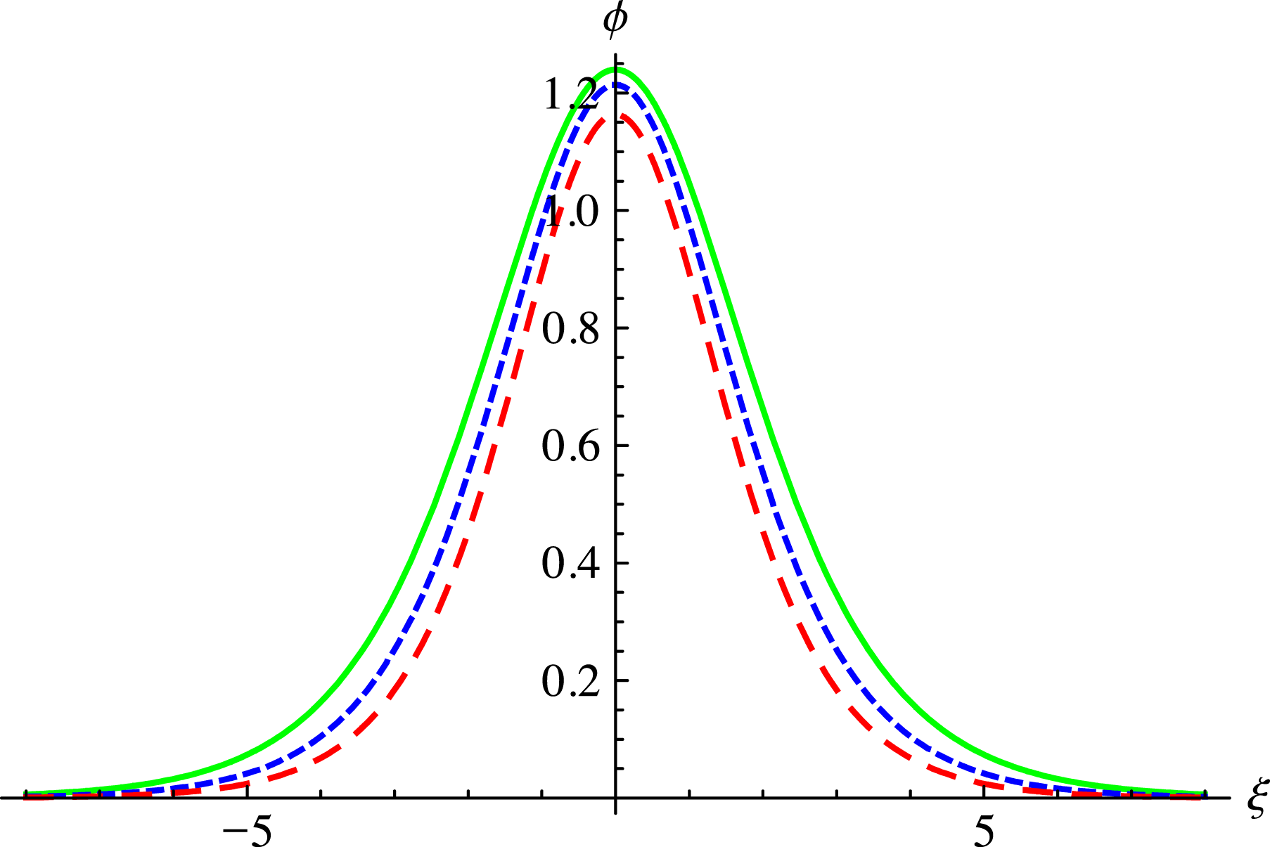
Solitary wave profile of (2.12) plotted for different ratios of electron and ion temperature,
 ${\it\beta}=1.1$
(green full curve),
 ${\it\beta}=1.3$
(blue dashed curve) and
 ${\it\beta}=1.5$
(red long dashed curve), with
 ${\it\alpha}=0.5,{\it\mu}=1837$
and
 $v=0.5$
.

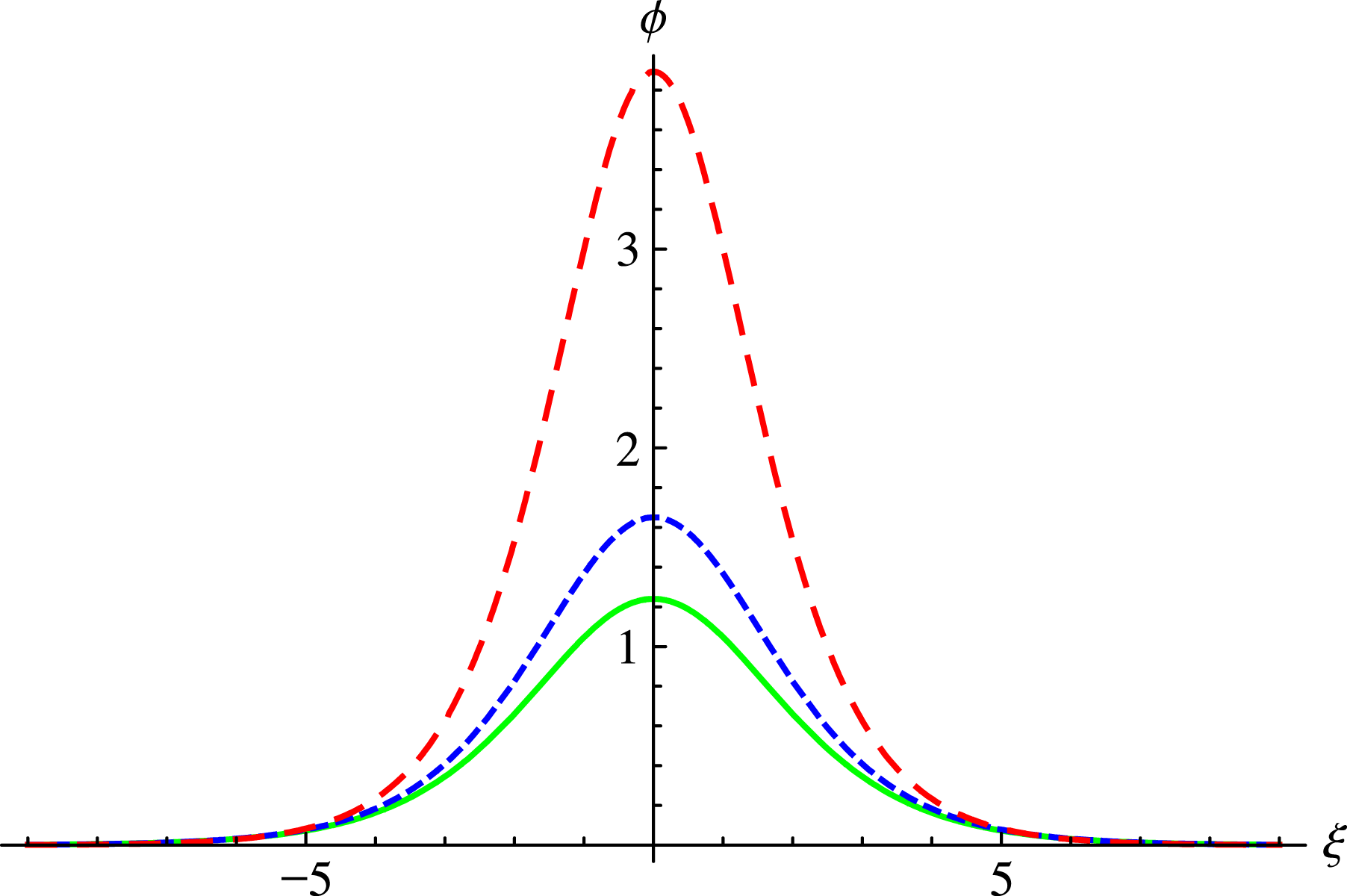
Solitary wave profile of (2.12) plotted for different values of the travelling wave speed,
 $v=0.5$
(green full curve),
 $v=0.51$
(blue dashed curve) and
 $v=0.52$
(red long dashed curve), with
 ${\it\alpha}=0.5,{\it\beta}=1.1$
and
 ${\it\mu}=1837$
.

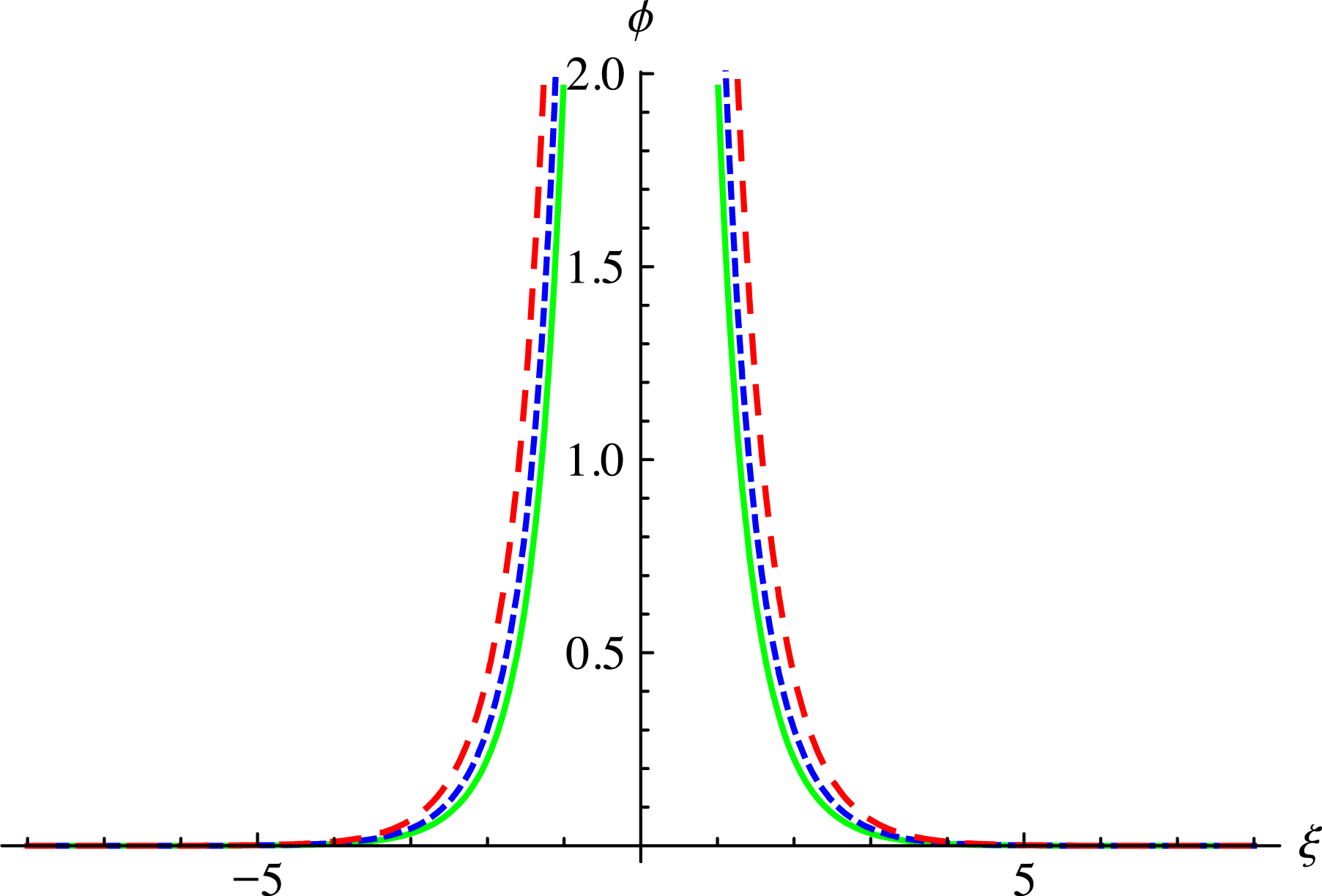
Blow-up solitary wave profile of (2.12) plotted for different ratios of electron and ion densities,
 ${\it\alpha}=0.3$
(green full curve),
 ${\it\alpha}=0.4$
(blue dashed curve) and
 ${\it\alpha}=0.5$
(red long dashed curve), with
 ${\it\beta}=1.9,{\it\mu}=1837$
and
 $v=2$
.

Blow-up solitary wave profile of (2.12) plotted for different ratios of electron and ion temperature,
 ${\it\beta}=1.5$
(green full curve),
 ${\it\beta}=1.7$
(blue dashed curve) and
 ${\it\beta}=1.9$
(red long dashed curve), with
 ${\it\alpha}=0.3,{\it\mu}=1837$
and
 $v=2$
.

5. Parametric effects
We now show the parametric effects of different physical parameters
 ${\it\alpha},{\it\beta},{\it\mu}$
and
 $v$
on the characteristics of dust acoustic solitary, blow-up solitary and periodic waves due to dust charge fluctuations.
Figure 5 provides information about the variation in amplitude and width of dust acoustic solitary waves (4.1) for different density ratios
 ${\it\alpha}$
of electrons and ions with fixed values of
 ${\it\beta},{\it\mu}$
and
 $v$
. The amplitude of dust acoustic solitary wave increases and the width of dust acoustic solitary wave decreases with increase in density ratio
 ${\it\alpha}$
of electrons and ions. Thus, the dust acoustic solitary wave becomes spiky as the density ratio
 ${\it\alpha}$
of electrons and ions is enhanced.
Figure 6 shows the variation of solitary wave profile (4.1) for different ratios
 ${\it\beta}$
of electron and ion temperature with fixed values of
 ${\it\alpha},{\it\mu}$
and
 $v$
. The amplitude and width of solitary waves decrease with increase in temperature ratio
 ${\it\beta}$
. Thus, the dust acoustic solitary wave is seen to diminish as the ratio of electron and ion temperature is enhanced.
Figure 7 shows the variation of solitary wave profile (4.1) for different values of
 $v$
with fixed values of
 ${\it\alpha},{\it\beta}$
and
 ${\it\mu}$
. The amplitude and width of solitary waves increase with increase in
 $v$
. Thus, the dust acoustic solitary wave is seen to flourish as the values of
 $v$
is enhanced.
Figure 8 provides information about the variation of dust acoustic blow-up solitary waves (4.2) for different density ratios
 ${\it\alpha}$
of electrons and ions with fixed values of
 ${\it\beta},{\it\mu}$
and
 $v$
. The width of dust acoustic blow-up solitary wave increases with increase in density ratio
 ${\it\alpha}$
of electrons and ions.
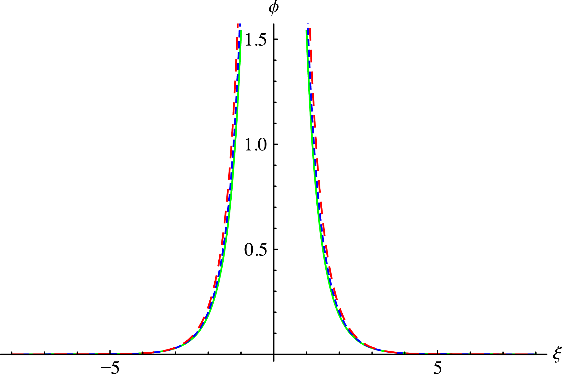
Blow-up solitary wave profile of (2.12) plotted for different values of the travelling wave speed,
 $v=2$
(green full curve),
 $v=3$
(blue dashed curve) and
 $v=4$
(red long dashed curve), with
 ${\it\alpha}=0.3,{\it\beta}=1.9$
and
 ${\it\mu}=1837$
.

Periodic wave profile of (2.12) plotted for different ratios of electron and ion densities,
 ${\it\alpha}=0.3$
(green full curve),
 ${\it\alpha}=0.33$
(blue dashed curve) and
 ${\it\alpha}=0.36$
(red long dashed curve), with
 ${\it\beta}=1.1,{\it\mu}=1837$
and
 $v=0.3$
.

Periodic wave profile of (2.12) plotted for different ratios of electron and ion temperature,
 ${\it\beta}=1.1$
(green full curve),
 ${\it\beta}=1.4$
(blue dashed curve) and
 ${\it\beta}=1.6$
(red long dashed curve), with
 ${\it\alpha}=0.3,{\it\mu}=1837$
and
 $v=0.3$
.

Periodic wave profile of (2.12) plotted for different values of the travelling wave speed,
 $v=0.3$
(green full curve),
 $v=0.305$
(blue dashed curve) and
 $v=0.31$
(red long dashed curve), with
 ${\it\alpha}=0.3,{\it\beta}=1.1$
and
 ${\it\mu}=1837$
.

Periodic wave profile of (2.12) plotted for different ratios of electron and ion densities,
 ${\it\alpha}=0.01$
(green full curve),
 ${\it\alpha}=0.013$
(blue dashed curve) and
 ${\it\alpha}=0.016$
(red long dashed curve), with
 ${\it\beta}=1.1,{\it\mu}=1837$
and
 $v=1$
.

Periodic wave profile of (2.12) plotted for different ratios of electron and ion temperature,
 ${\it\beta}=1.1$
(green full curve),
 ${\it\beta}=1.2$
(blue dashed curve) and
 ${\it\beta}=1.3$
(red long dashed curve), with
 ${\it\alpha}=0.01,{\it\mu}=1837$
and
 $v=1$
.

Periodic wave profile of (2.12) plotted for different values of the travelling wave speed,
 $v=1$
(green full curve),
 $v=1.2$
(blue dashed curve) and
 $v=1.4$
(red long dashed curve), with
 ${\it\alpha}=0.01,{\it\beta}=1.1$
and
 ${\it\mu}=1837$
.

Figure 9 shows the variation of dust acoustic blow-up solitary waves (4.2) for different ratios
 ${\it\beta}$
of electron and ion temperature with fixed values of
 ${\it\alpha},{\it\mu}$
and
 $v$
. The width of dust acoustic blow-up solitary waves increases with increase in temperature ratio
 ${\it\beta}$
.
Figure 10 shows the variation of dust acoustic blow-up solitary waves (4.2) for different values of
 $v$
with fixed values of
 ${\it\alpha},{\it\beta}$
and
 ${\it\mu}$
. The width of dust acoustic blow-up solitary waves decreases with increase in
 $v$
.
Figure 11 provides information about the variation in amplitude and width of dust acoustic periodic waves (4.3) for different density ratios
 ${\it\alpha}$
of electrons and ions with fixed values of
 ${\it\beta},{\it\mu}$
and
 $v$
. The amplitude and width of dust acoustic periodic wave increase with increase in density ratio
 ${\it\alpha}$
of electrons and ions. Thus, the dust acoustic periodic wave is seen to flourish as the value of
 ${\it\alpha}$
is enhanced.
Figure 12 shows the variation of periodic wave profile (4.3) for different ratios
 ${\it\beta}$
of electron and ion temperature with fixed values of
 ${\it\alpha},{\it\mu}$
and
 $v$
. The amplitude and width of solitary waves increase with increase in temperature ratio
 ${\it\beta}$
. Thus, the dust acoustic periodic wave is seen to flourish as the ratio of electron and ion temperature is enhanced.
Figure 13 shows the variation of dust acoustic periodic wave profile (4.3) for different values of
 $v$
with fixed values of
 ${\it\alpha},{\it\beta}$
and
 ${\it\mu}$
. The amplitude and width of dust acoustic periodic waves increase with increase in
 $v$
. Thus, the dust acoustic periodic wave is seen to flourish as the value of
 $v$
is enhanced.
Figure 14 provides information about the variation in amplitude and width of dust acoustic periodic waves (4.4) for different density ratios
 ${\it\alpha}$
of electrons and ions with fixed values of
 ${\it\beta},{\it\mu}$
and
 $v$
. The amplitude and width of dust acoustic periodic wave decrease with increase in density ratio
 ${\it\alpha}$
of electrons and ions. Thus, the dust acoustic periodic wave is seen to diminish as the value of
 ${\it\alpha}$
is enhanced.
Figure 15 shows the variation of periodic wave profile (4.4) for different ratios
 ${\it\beta}$
of electron and ion temperature with fixed values of
 ${\it\alpha},{\it\mu}$
and
 $v$
. The amplitude of dust acoustic periodic wave increases and the width of dust acoustic periodic wave decreases with increase in temperature ratio
 ${\it\beta}$
. Thus, the dust acoustic periodic wave becomes spiky as the ratio of electron and ion temperature is enhanced.
Figure 16 shows the variation of dust acoustic periodic wave profile (4.4) for different values of
 $v$
with fixed values of
 ${\it\alpha},{\it\beta}$
and
 ${\it\mu}$
. The amplitude and width of the periodic waves decrease with increase in
 $v$
. Thus, the dust acoustic periodic wave is seen to diminish as the value of
 $v$
is enhanced.
6. Conclusions
We have addressed dust acoustic solitary waves, blow-up solitary waves and periodic waves in an unmagnetized dusty plasma with Maxwell-distributed electrons and ions in the presence of variable dust charge. Applying the bifurcation theory of planar dynamical systems, we have proved that our model has a solitary wave solution, a blow-up solitary wave solution and periodic travelling wave solutions. Analytical solutions for solitary, blow-up solitary and periodic waves are obtained using the dynamical system (2.13) and the Hamiltonian function given by (2.14). From these analytical solutions, the effects of the density ratio of electrons and ions (
 ${\it\alpha}$
), the temperature ratio of electrons and ions (
 ${\it\beta}$
) and the speed of the travelling wave (
 $v$
) on the characteristics of dust acoustic solitary, blow-up solitary and periodic waves are presented. The parameters
 ${\it\alpha},{\it\beta}$
and
 $v$
significantly affect the characteristics of dust acoustic solitary, blow-up solitary and periodic structures. Our present investigation may be helpful in understanding the salient features of the nonlinear solitary and periodic structures in space plasma environments (Verheest Reference Verheest2000), where the dust acoustic wave frequency and the dust charging frequency are comparable.
Acknowledgements
This work is partially supported by DST, India (under D.O. no. SR/S2/HEP-32/2012). The authors are really grateful to the reviewers for their useful comments and suggestions, which helped to improve the paper.