Advances in scanning transmission electron microscopy

Materials underpin civilization, ranging from structural materials used to build higher buildings and faster, longer-lived, and multifunctional machines, to the batteries and fuel cells that power them, and from the semiconductors that constitute modern electronics, to biomaterials that promise to open new chapters in medicine and biotechnology. Correspondingly, making materials better and cheaper and developing materials with new functionalities are central tasks for the aspiring materials scientist. Similarly, explosive growth in quantum materials and devices and approaching the limits of Moore’s Law in electronics (where the number of transistors incorporated in a chip will approximately double every two years) in the last several years has started to lower the barriers between top-down and bottom-up synthesis approaches, with the size of classical semiconductor electronics approaching the single-digit nanometer length scales of large clusters, and single atom and single defect qubits and devices becoming a rapidly developing technological paradigm.

Progress in materials science is inseparable from the development of new methods and ideas. Materials science emerged as a result of the gradual cross-pollination between classical 19th century disciplines, such as ceramics, metallurgy, and glass science, and condensed-matter physics of the mid-20th century.^{Reference Martin1} Much of this progress was aided by the development of imaging tools, notably electron and scanning probe microscopes, which provided deep insights into microstructures and mechanisms responsible for materials functionalities. Examples as diverse as dislocation dynamics during plastic deformation, ferroelectric domain dynamics during switching, formation of nanoscale phase separated states in relaxors, superconductors, and metal–insulator systems have provided insight into the associated functionalities and have stimulated new generations of theory (or pointed to the need of new models beyond macroscopic theories). However, until now, both scanning probe microscopy (SPM) and electron microscopy communities have been heavily focused on instrument development and qualitative interpretations.^{Reference Mody2}

Yet, at certain junctions, the normally slow progress in instrumentation is interspersed with revolutions, giving rise to fundamentally new concepts and opportunities. In scanning transmission electron microscopy (STEM), the practical realization of aberration correction by Krivanek et al.^{Reference Krivanek, Dellby, Spence, Camps, Brown and Rodenburg3} (and by Haider et al. in the TEM^{Reference Haider, Uhlemann, Schwan, Rose, Kabius and Urban4}) has given rise to a cascade of developments, the impact of which is only now being fully appreciated.

Briefly, the fundamental principles of electron optics impose a limit on achievable resolution for the electron beam—provided that the beam is cylindrically symmetric. This limitation can be circumvented by breaking rotational symmetry, as was proposed more than 50 years ago by Scherzer.^{Reference Scherzer5} However, the practical realization of aberration correction had to wait for the development of sufficiently powerful computers, capable of performing the automatic tuning of tens of lens elements.^{Reference Dellby, Krivanek, Nellist, Batson and Lupini6} Once implemented, however, aberration correction opened a treasure trove of high-resolution observation data. Perhaps the key benefit being that for common medium-energy (40–300 keV) electron microscopes, the “typical” resolution advanced from slightly worse to noticeably better than atomic resolution.

The structures of objects such as grain boundaries in SrTiO₃ and superconductors, and quasicrystals, were suddenly available for exploration in detail, providing high-clarity images where once only poorly resolved images had been available.^{Reference Pennycook and Nellist7} Within less than a decade, this opened the pathway for quantitative studies of the physics of solids. These developments further led to advances in associated spectroscopic techniques, in particular electron energy-loss spectroscopy. Advances in sensitivity and spatial resolution have enabled single-atom spectroscopy^{Reference Varela, Findlay, Lupini, Christen, Borisevich, Dellby, Krivanek, Nellist, Oxley, Allen and Pennycook8} and have further enabled nearly routine probing of chemical composition, electronic properties, and oxidation states in a broad range of materials. This, in turn, enabled quantitative studies of coupled physical and electrochemical processes in multiple materials (e.g., oxide interfaces, batteries, fuel cells, and even ferroelectric domain walls). The addition of monochromation has further pushed the energy resolution to the ∼meV regime,^{Reference Idrobo, Lupini, Feng, Unocic, Walden, Gardiner, Lovejoy, Dellby, Pantelides and Krivanek9} opening the vibrational properties of solids and molecular structures for exploration.

Recent developments that are capturing the attention of the STEM community include vortex beams^{Reference Larocque, Bouchard, Grillo, Sit, Frabboni, Dunin-Borkowski, Padgett, Boyd and Karimi10} capable of probing local magnetism, ferrotoroid properties, orbital orderings, and four-dimensional (4D) STEM based on subatomic diffraction imaging.^{Reference Jiang, Chen, Hang, Deb, Gao, Xie, Purohit, Tate, Park, Gruner, Elser and Muller11} Most recently, groups at Oak Ridge National Laboratory (ORNL) and the University of Vienna have experimentally demonstrated that the electron beam in a STEM can be used to manipulate single atoms and assemble structures atom by atom,^{Reference Dyck, Kim, Jimenez-Izal, Alexandrova, Kalinin and Jesse12,Reference Susi, Meyer and Kotakoski13} similar to scanning tunneling microscopy (STM) three decades ago.^{Reference Eigler and Schweizer14} The impact of these developments is amplified by the availability of hundreds of commercial microscopes that can now operate as small imaging facilities in academia, national labs, and industry and are available for broad communities via user centers.

The impact of these developments has propelled the STEM beyond being a mere imaging tool, settling the discussions for the need for high-resolution machines that started since the days of Gabor and have continued recently.^{Reference Pennycook and Kalinin15} Currently, STEM is becoming a quantitative tool capable of probing atomic coordinates with picometer precision, providing high veracity information on electronic, plasmonic, and vibrational properties, and even allowing for controllable modification of solid structures. Correspondingly, a new set of questions has emerged:

1. 1. What can we do with these data?

2. 2. How can we use them for making better materials?

3. 3. Can we understand fundamental physics, including quantifying known interactions and mechanisms and discovering new ones, based on these data?

4. 4. Ultimately, can we transition from imaging to manipulation of matter at the atomic limit?

Challenges for STEM

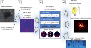
The challenges facing researchers in the STEM, materials, and condensed-matter physics communities are fourfold (Figure 1).^{Reference Ziatdinov, Dyck, Jesse and Kalinin16,Reference Jesse, He, Lupini, Leonard, Oxley, Ovchinnikov, Unocic, Tselev, Fuentes-Cabrera, Sumpter, Pennycook, Kalinin and Borisevich17} The first challenge is whether materials-specific information (e.g., atomic coordinates from STEM, scattering potentials from 4D STEM) can be obtained from microscopy data, at which level of confidence, and how this knowledge is affected by and can be improved from knowledge of an imaging system (e.g., classical beam parameters, resolution function, all the way to full imaging system modeling) and knowledge of the material. Note that a significant advantage of Z-contrast STEM is that the contrast is more directly associated with the position of atomic nuclei, as compared to the considerably more complex contrast formation mechanisms in conventional TEM and atomically resolved SPM. It is largely this ease of interpretation that attracted the attention of physicists and materials scientists to this instrument, and, significantly, which may no longer be the case for the interpretation of 4D STEM and vortex beams.

Figure 1.

The four challenges for atomically resolved imaging. (a) Starting with data flow from the detector and (b) using (partial) knowledge of the imaging system and material (in this example, graphene with impurities), we aim to obtain material-specific information (e.g., type and positions of individual atoms).^{Reference Ziatdinov, Dyck, Jesse and Kalinin16} (c) From this (partial) materials-specific information, we aim to generate correlative or causative knowledge about materials behavior (e.g., defect libraries or constitutive equations describing materials behavior).^{Reference Ziatdinov, Dyck, Jesse and Kalinin16} (d) With this information in hand, we can predict materials functionalities in the broad parameter space or use it as feedback during microscope operation.^{Reference Jesse, He, Lupini, Leonard, Oxley, Ovchinnikov, Unocic, Tselev, Fuentes-Cabrera, Sumpter, Pennycook, Kalinin and Borisevich17} Shown for illustrative purposes in (c) are the bipartite lattice Hamiltonian (with a ^†/a being creation/annihilation operators of spin σ (σ = ↑↓) at site i of the sublattice A and t being the nearest neighbor hopping energy) and force field (with k being a force constant, and l and θ being bonds and angles, respectively) equations, while the exact form of modeling equations may be different for different systems and applications.

The second challenge is whether materials-specific information with uncertainties determined by incomplete knowledge of the imaging system or intrinsic limitations of the imaging process can be used to infer physics and chemistry, via either correlative models or recovery of generative physics (force fields, exchange integrals). Assuming that we possess information on the position of all (or a significant number of) atoms in a given volume of material, what conclusions can we derive on the physics and chemistry of the material? Similarly, if certain types of responses are associated with particular structural elements, what does this tell us about the material?

The third challenge is whether the determined materials information, either correlative or causative, can be used to reconstruct materials behaviors (phase diagrams, properties) in the broader parameter space (e.g., for temperatures and concentrations different to the specific sample studied) and to determine how the reliability of such predictions depends on position in parameter space. In other words, how far can we generalize from the information we derive?

The fourth challenge is whether we can harness the data stream from the microscope to engender real-time feedback (e.g., for autonomous experimentation and atomic manipulation).

The first of these challenges lies firmly in the domain of the instrumental STEM community and provides the impetus for the continuous development of microscopic tools and data analysis methods. Instrument development and forward modeling are being undertaken by multiple research centers and commercial entities worldwide and are generally well underway. What is often missing is the uncertainty quantification in data interpretation (i.e., what are the instrument-imposed uncertainties in materials properties—for example, atomic coordinates—obtained from the data)? This knowledge is necessary since physics is often related to the subtle details of symmetry breaking or local responses. Although for macroscopically uniform systems, scattering methods often will provide the missing or corroborative information, the primary application for imaging methods are physics and chemistry of local phenomena, where such verification can be impossible.

Image recognition tools and machine learning

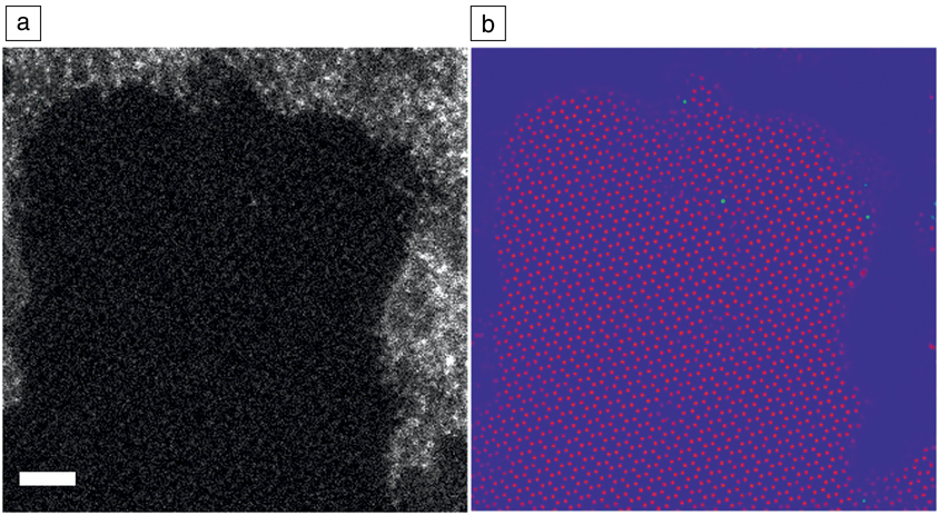
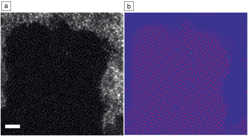
At this stage, machine learning and image recognition tools can be of immense utility. For example, a typical task that underpins virtually all materials-specific analysis is the conversion of a STEM image or movie into a set of atomic coordinates or trajectories. A large number of approaches have been suggested for this, ranging from Fourier-based methods to local contrast enhancement, to more sophisticated tools based on Hough transforms and local clustering. However, most of these techniques demonstrate performance roughly comparable to the visual recognition by a trained operator. As in many areas, the introduction of deep-learning methods based on the convolutional neural networks has demonstrated uncanny efficiency in these tasks, as illustrated in Figure 2, as well as in ancillary tasks such as drift correction and denoising. Currently, intensive research is underway to establish whether these approaches can be used for more complex tasks (e.g., inversion of 4D STEM data to details of the projected scattering potential or to recover 3D atomic coordinates).

Figure 2.

Application of deep-learning networks for feature finding and image inversion. (a) Scanning transmission electron microscope image of Si adatoms on graphene in the presence of contaminants. Scale bar = 1 nm. The data show graphene lattice (darker regions with periodic pattern), amorphous SiC regions (larger brighter regions), and point Si dopants in graphene lattice (isolated bright spots). (b) Deep-learning analytics of the image in (a). Green corresponds to Si atoms, red to carbon. The output represents the probability density that a certain pixel belongs to a particular atom type. Note the robustness of the network to noise, when the locations of carbon atoms are identified above the human eye perception. The open codes for these analyses are available on the PyCroscopy domain on GitHub.²⁰ Data courtesy of O. Dyck.

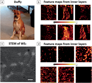
Notably, this conversion of image data to materials-specific information can be greatly assisted by partial knowledge of the materials structure. For example, Fourier methods explicitly rely on the periodicity of the material and implicitly assume that they are not affected by the presence of point defects (they often fail where the periodicity is piecewise continuous, necessitating the development of appropriate segmentation methods). Most local contrast analyses rely on the knowledge that contrast maxima correspond to atomic features, and the features have certain characteristic sizes and spacing. These assumptions can be quantified via the use of corresponding Bayesian methods, as demonstrated recently for STEM^{Reference Feng, Kvit, Zhang, Hoffman, Bhattacharya, Morgan and Voyles18} and STM.^{Reference Ziatdinov, Maksov and Kalinin19} In deep-learning methods, the choice of the training set allows one to encode prior knowledge of possible materials structures, imposing a form of regularization on the feature finding process. As shown by Ziatdinov²⁰ (Figure 3),^{Reference Simonyan and Zisserman21,22} a deep-learning network trained to find “dogs and cats” would still find them even in atomically resolved images of 2D materials. At the same time, a neural net trained to recognize atomic defects or atomic species can perform better and far faster than a human operator and in a robust and automated fashion.^{Reference Ziatdinov, Dyck, Maksov, Li, Sang, Xiao, Unocic, Vasudevan, Jesse and Kalinin23–Reference Rashidi and Wolkow26} This performance, when combined with new open-source software (such as Nion Swift^{Reference Swift27}), allows these networks to be deployed as real-time analysis tools.

Figure 3.

Illustration of the potential pitfall of deep-learning analytics of experimental images. (a) The pretrained (on the standard image collection) Visual Geometry Group (VGG)-19²¹ deep-learning network can immediately identify the dog in the photo (Pit Bull-Shepherd-Collie mix) and even establish its breed as Staffordshire bull terrier (43%), American pit bull terrier (23%), and Basenji (11%). The neural network achieves this by learning features directly from the raw data. It first locates an object by finding its contours and then learns finer features associated in this case with the dog’s body structure and the shape of its ears, nose, etc., which allows a network to identify the dog’s breed. (b) Some of the feature maps learned by the inner layers of VGG neural network. These feature maps can provide some insight into how a network learns that there is a dog in the image. However, the use of this network for the atomically resolved images such as (c) a scanning transmission electron microscope experiment on WS₂ yielded spurious identification as (d) wool (6.3%), chain mail, or velvet , simply because the network was not trained on such images. It also becomes quite obvious that a network trained on a standard set of images deals with experimental noise poorly (despite being a powerful feature extractor, it cannot extract meaningful features of an atomic lattice as can be seen from (d). Correspondingly, choice of the proper training set representing possible materials microstructures and microscope parameter uncertainties become the primary issue in successful applications of deep learning in image analytics. The feature maps in (b) and (d) are obtained from the eighth layer of the VGG-19 network (the total number of feature maps in this layer is 256, and then it becomes 512 in the next one). Notice that because the image size is reduced by a factor of 2 multiple times as it moves through a network, the feature maps in the next layers become too small for meaningful (to humans) visualization. (c) Scale bar = 1 nm. Image of dog Duffy is courtesy of M. Ziatdinov. Readers can perform this analysis themselves (with their own images and their own experimental data) using our notebook (see Reference 22).

The availability of large volumes of structural information enabled by automatic image processing will allow us to considerably expand our knowledge of materials. For example, observations of point and extended defects in layered materials, for the equilibrium structure of the material, as well as those emerging as a result of electron irradiation, have recently been achieved.^{Reference Krivanek, Chisholm, Nicolosi, Pennycook, Corbin, Dellby, Murfitt, Own, Szilagyi, Oxley, Pantelides and Pennycook28} Analysis of large volumes of such data enable the creation of defect libraries that contain information on the types and populations of the individual defects and potentially their properties and interactions. Naturally, defect populations in solids are fundamentally linked to the thermodynamics and kinetics of solid-state (electro) chemistry, providing atomistic insights into the latter.

Rajan et al. ^{Reference Govind Rajan, Silmore, Swett, Robertson, Warner, Blankschtein and Strano29} demonstrated a method for creating a theoretical library of nano-sized pore defects in 2D materials and exploring their energetics. Knowledge of defect populations opens the pathway for cross-correlative studies (i.e., via imaging by complementary techniques). Ziatdinov et al.^{Reference Ziatdinov, Dyck, Sumpter, Jesse, Vasudevan and Kalinin30} recently demonstrated the creation of a defect library for Si atoms in graphene and predicted the electronic signatures of defects via density functional modeling, further verifying STM observations of the same material. These images are now saved in an open data repository on a Citrination platform.³¹

Perhaps the most interesting challenge facing the microscopy and physics communities is what information on materials physics can be obtained from such data? Indeed, observations of near-surface relaxations and ferroic orderings on multiple materials have been reported, showing broad variability of behaviors due to the interplay among physical, chemical, and morphological effects. Yet the underpinning physics often can be represented in terms of low-dimensional depictions, such as characteristic energies and interaction potentials and force fields. The question is whether such generalizable low-dimensional representations can be extracted from observations of multiple spatially resolved degrees of freedom. A pertinent comparison in this case is with the field of astronomy, where (due to the obvious and perhaps fortuitous lack of experimental capabilities) involved models of the universe are obtained from observations rather than large-scale experiments.

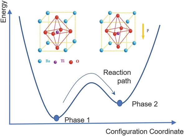
This challenge can be further understood from the following example. Often the macroscopic physics of solids is illustrated by simplified schemes, as for the case of ferroelectric materials in Figure 4. Here, the energy of the system is represented as a function of a certain collective variable (order parameter) that determines the free energy of the system and can be unambiguously related to the structural properties and symmetry changes across the phase transition. However, the macroscopic (and even microscopic) volumes contain large numbers of atomic units, and the representations, such as in Figure 4, demonstrate the collective effects of multiple units.

Figure 4.

Physics of ferroelectric materials is often illustrated via the concept of double well potential, with potential energy minima corresponding to antiparallel polarization orientations. This picture naturally presents the switching process via the addition of an extra PE term (P is polarization and E is electric field) representing the coupling with the external field. However, while the vertical axis has a straightforward meaning, the horizontal axis is a collective variable representing collective dynamics of all unit cells within the material. Inset shows (left) a high symmetry unpolled state and (right) lower symmetry poled state of a BiTeO₃ ferroelectric material.

Phase-field theories based on the free-energy expansion in powers of order parameters are a powerful tool to describe materials properties and structure, topological defects, and emergence of new functionalities. Yet while bulk components are often well understood, the nature of the terms defining order parameter behaviors at interfaces and surfaces (boundary conditions) and gradient terms are often unknown and cannot be determined from the mesoscopic theory. Similarly, for materials possessing frustrated ground states (i.e., due to competing symmetry-incompatible interactions) or large disorder, the appropriateness of order parameter-based descriptions is continuously debated. These include ferroelectric relaxors, materials at the morphotropic phase boundaries, Kitaev spin liquids,^{Reference Takagi, Takayama, Jackeli, Khaliullin and Nagler32} and phase-separated oxides. Naturally, these are the materials of a strong interest to the materials community, both due to the fundamental physics challenges they offer and to the unique functional properties they possess (e.g., giant magnetoresistance in manganites or giant electromechanical coupling in relaxors).

Materials properties from observations

One approach for extracting materials-specific properties from atomically resolved data is based on matching to mesoscopic models. For materials with well-known (from macroscopic measurements) free-energy functional and unknown forms of boundary conditions at surfaces, interfaces, and defects, analytical solutions for order parameter profiles can be derived and further fitted to experimental data. This approach was used for describing antiphase boundaries in vacancy-ordered brownmillerites (materials having a structure of brownmillerite Ca₂(Al,Fe)₂O₅)^{Reference Borisevich, Morozovska, Kim, Leonard, Oxley, Biegalski, Eliseev and Kalinin33} and flexoelectric coupling from the shape of vortex defects in lead titanate.^{Reference Li, Nelson, Hsu, Damodaran, Li, Yadav, McCarter, Martin, Ramesh and Kalinin34} Multiple solutions for domain walls and other topological defects are available, allowing further extension of this approach to cases where only numerical solutions are available (i.e., due to complex geometries). This approach can also be used in more complex cases, where analytical solutions using numerical schemes are absent.

Similar analyses can be performed for dynamic observations. Many observations of dynamic processes, including electrochemistry of batteries and dendrite formation, have been reported. However, of interest is the extraction of the relevant mesoscopic descriptors (e.g., reaction and diffusion rates, orientation-dependent free energies). Recently, such an approach was demonstrated for electrochemical deposition, where matching of the experimentally observed particle growth rates with those calculated from the experimental geometry was used to determine the reaction and diffusion rates.^{Reference Ievlev, Jesse, Cochell, Unocic, Protopopescu and Kalinin35} Similar approaches can be used for other dynamics processes, including ferroelectric domain growth.

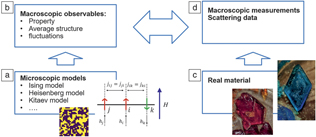
The analysis of materials properties can be performed on a deeper level by directly analyzing atomically resolved degrees of freedom to extract pairwise interactions (Figure 5). For example, many physical descriptors of solids rely on lattice-based models, where individual degrees of freedom of atoms in the lattice are represented by “spins” interacting with each other via local interactions and are affected by macroscopic fields. The simplest example of such a model is the Ising model, where spins have up and down states; there are more complex models including the Heisenberg and Potts models.^{Reference Sethna36} Despite their apparent simplicity, many of these models can give rise to complex phase diagrams and behaviors, making them a traditional object of study for condensed-matter physics.

Figure 5.

(a) Traditionally, microscopic lattice and off-lattice models are used to (b) derive macroscopic properties and structures, (c) which can be further compared with experimental observations (d). We pose that the microscopic degrees of freedom from the scanning transmission electron microscope or scanning tunneling microscope experiment can be directly matched to the microscopic lattice- and off-lattice models, yielding the information on local interactions. In (a), j, i, and k are the “spin” lattice sites, j _ij denotes “spin–spin” (exchange) interaction, and h _i denotes “spin” interaction with external field H. The inset in (a) shows a snapshot of classical 2D Ising lattice at finite temperature. Photos of (left) CuSO₄ and (right) K₃[Fe(CN)₆] crystals are courtesy of A.S. Kalinin and D.S. Kalinin.

Of interest is how the relationship between specific materials and the corresponding lattice model is established. In most cases, theorists explore the behavior of a specific model, including phase diagrams in parameter space (e.g., temperature, field, strength of individual interactions) and macroscopic responses such as susceptibilities and heat capacities. From the experimental side, similar properties can be measured experimentally via macroscopic measurements and structural probes. Establishing the proper model for a specific material can be controversial. However, once the model is selected, the comparison of macroscopic observables allows determination of the local interactions, with the underlying assumption that there is a unique correspondence of a certain class of local structures to the global macroscopic observables. Moreover, it implies that many macroscopic measurements need to be made to explore the full phase diagram, generally leading to community-wide efforts that span years, especially for complex systems (such as manganites).

Local observations

In the context of STEM and other atomically resolved imaging methods, the local degrees of freedom are directly amenable for observation. Correspondingly, the natural question is whether the model parameters can be determined from such local observations, and thereby provide the lattice Hamiltonian that describes the system’s states. An example of such an approach is illustrated in Figure 6.^{Reference Vlcek, Maksov, Pan, Vasudevan and Kalinin37} Here, the STM image of the layered semiconductor FeSe_0.45Te_0.55 surface illustrates the presence of two types of atomic species (Se and Te). Direct examination of the image shows that the atomic distributions are not random, and, in fact, atoms of similar types have a profound tendency to segregate and form light and dark atom clusters. This behavior can be easily reproduced using simple statistical models, such as a nonideal solid solution, where the preferential tendency for atoms of the same kind to segregate is described by a single parameter.

Figure 6.

(a, upper) Scanning tunneling microscope image of an FeSe_0.45Te_0.55 surface with bright and dark atoms representing Se and Te, respectively. Scale bar = 3 nm. (Lower) A schematic of the layered FeSe lattice structure. (b) A lattice model is initialized with effective interactions between the different atomic species present. $w_x^p$ are the interaction parameters in system p, and quantity ${{\rm{\delta }}^x}$ is equal either to one of the interactions between particles defined by ${w_x}$ or zero. (c) Statistics of atomic configurations are computed from the experimental images (blue vertical bars in histogram; the configurations themselves are shown in the top panel, where Se and Te atoms are blue and red, respectively) and from the model (red vertical bars in histogram) and compared. The statistical distance metric between the two histograms in (c) (one from experiment, one from the model) is minimized by tuning the interaction parameters of the statistical model. Once the model is optimized in this manner, it can be used for predictions at unseen thermodynamic conditions as illustrated in (d) for reduced temperatures of ${T^*} = 0.75$ and ${T^*} = 1$ (consistent with experimental data) at Se concentration of 0.45. Note: h _anion, anion height (distance between the Fe layer and anion); σ_A, unit cell area; P _i, probability of finding outcome i in the measurement of the system p; NN, nearest neighbors; u _i, energy of configuration i.^{Reference Vlcek, Maksov, Pan, Vasudevan and Kalinin37}

In this specific case, the question is whether this parameter (and its associated uncertainty) can be extracted from the experimental observations. The approach for such analysis was developed by Vlcek^{Reference Vlcek, Vasudevan, Jesse and Kalinin38} and was demonstrated for layered semiconductors and manganites.^{Reference Vlcek, Maksov, Pan, Vasudevan and Kalinin37,Reference Vlcek, Ziatdinov, Maksov, Tselev, Baddorf, Kalinin and Vasudevan39} It relies on the principles of equilibrium thermodynamics and essentially optimizes a model’s parameters to best represent the distributions found in experiments. After optimization, taking samples from the model would be indistinguishable from drawing samples from experiments and allows the model to have predictive power. Notable is that the local interactions extracted from the image(s) of a single composition can further be used to explore a much broader parameter space of the material and ultimately reconstruct the associated phase diagram. Moreover, this approach lends immediately to uncertainty quantification under a Bayesian framework (a statistical approach to uncertainty where beliefs, called priors, are updated based on observations), where the goal is not only to determine the mean of the interaction parameters, but also to infer the most probable form of the distributions. Sampling from these distributions to produce phase diagrams then allows for calculation of the uncertainty at each point in the thermodynamic space.

The challenge of material description becomes considerably more complex for structures with broken lattice periodicity, especially for dynamic systems. Here, the fundamental challenge is the nature of the local structural materials descriptors as a first step for exploring correlation with local properties and developing causative models. As discussed previously, for periodic solids, such descriptors can be naturally constructed based on the symmetry properties of the lattice. In comparison, for molecular systems, the descriptors based on atomic connectivity and identities have been developed for several decades. For specific processes, the multiple molecular degrees of freedom can be represented as a smaller number of reaction coordinates and slow degrees of freedom (i.e., characteristic elements of molecular structure that evolve only slowly with time, similar to those illustrated in Figure 4); however, analysis of these represents one of the ongoing challenges in computational chemistry. In comparison, analysis of defects in solids represents an even more complex task, since in this case, even defects with nominally identical bonding patterns can be distorted because of the presence of nonlocal strain and electric fields.

However, in several cases, the analysis can be straightforward and achieved by direct application of well-established chemical concepts. Figure 7 illustrates the evolution of the structure of single-layer WS₂ under the action of an electron beam.^{Reference Maksov, Dyck, Wang, Xiao, Geohegan, Sumpter, Vasudevan, Jesse, Kalinin and Ziatdinov24} During this process, the electrons remove individual chalcogen atoms. This process has a small cross section, and only a few atoms are removed in each image. Combining with the fast (femtosecond) time scale of the electron passage, this allows us to represent the degradation process as a slow reduction observed at atomic resolution. Correspondingly, we observed formation of point defects, gradual aggregation and formation of extended defects and holes, and continuous degradation of the material. Since only point defects form at the early stage of the process, long-range lattice periodicity is initially maintained. In this case, the use of a deep-learning-based framework allows for the reconstruction of individual defect positions within an image frame that can further (after compensating for drift) be represented as space–time trajectories. Several characteristic defect types were identified. For sulfur vacancies, the diffusion coefficient could be extracted. For static molybdenum dopants, the kinetics of formation and isomerization of the Mo_W–S_vac complex (i.e., Mo on W site forming a pair with a sulfur vacancy) could be established.^{Reference Maksov, Dyck, Wang, Xiao, Geohegan, Sumpter, Vasudevan, Jesse, Kalinin and Ziatdinov24}

Figure 7.

(a) Experimental scanning transmission electron microscope movie of degradation of WS₂ under electron-beam irradiation. The left and right frames were obtained on the same area at ∼90 s and ∼200 s, respectively, after the start of irradiation. The degradation of the material within this ∼110 s time period can be clearly seen. Scale bars = 2 nm. (b) Spatiotemporal trajectories reconstructed from the raw data using a combination of a deep-learning network (defect localization) and a Gaussian mixture model (defect classification). Here, Class 4 and Class 5 are associated with W vacancy and S/S₂ vacancies, respectively, Classes 1 and 3 are associated with Mo dopants coupled to a S vacancy, and Class 2 corresponds to “contaminations” (the exact nature of which has not yet been explored in detail). One can identify multiple well-defined trajectories consisting either mostly of a single defect class or multiple defect classes. These trajectories can be isolated and used for an in-depth study of defect dynamics and transformations as illustrated in (c–g). (c, d) One-dimensional representation of trajectories (c) of defect subclasses originating from additional splitting of classes 1 and 3 in (b) and associated with (d) different types of Mo dopant coupling to S vacancy and with a single Mo dopant. The color scheme in (c) is the same as used for different defects in (d). Note: I, II, and III, different rotational states of the (Mo_W + V_S structure). (e, f) These trajectories are used for Markov analysis. Specifically, (e) shows a schematic of Markov transition processes for a four-state system. Each state can transition either into itself or into one of the other three states. (f) Transition probabilities calculated from the trajectories in (c). Different colors are associated with calculated values of transition probabilities. (g) A calculation of diffusion coefficient D for defect class associated with S vacancies (shown in inset; “0” and “1” denote two different trajectories) within the 2D random walk approximation from the corresponding trajectories, isolated and collapsed onto a 2D plane. Overall, this figure shows how point-defect dynamics and solid-state transformations in the material under electron-beam irradiation (or other stimuli) can be accessed on the atomic level and corresponding reaction constants can be determined for just one point defect. Note: r, 1D representation of coordinates ($\sqrt {{X^2} + {Y^2}}$); Mo_W, Mo on W site; V_S, sulfur vacancy.^{Reference Maksov, Dyck, Wang, Xiao, Geohegan, Sumpter, Vasudevan, Jesse, Kalinin and Ziatdinov24}

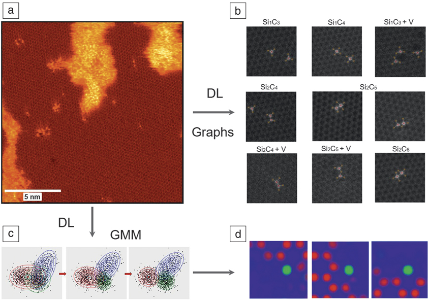
In other cases, establishing the state descriptors represents a more complex problem. For Si in carbon dynamics, these descriptors were derived based on a Gaussian mixture analysis of the images, and corresponding transition rates were determined using Markov chain models. Alternatively, libraries of defects can be established via graph segmentation analysis, as illustrated in Figure 8. However, both the establishment of structural descriptors and reaction and transformation pathways remain as open problems. For ergodic processes, Markov models offer a good start. For more complex and nonequilibrium cases, more complex Koopman formalism or VAMPNets^{Reference Mardt, Pasquali, Wu and Noe40} can offer a way forward.

Figure 8.

Schematics of learning structural descriptors from scanning transmission electron microscope (STEM) data. (a) Experimental STEM image of graphene with Si impurities. Darker areas are graphene lattice, larger brighter areas are Si-C amorphous regions, and smaller bright clusters and individual bright spots are Si-C defect complexes of interest.^{Reference Ziatdinov, Dyck, Sumpter, Jesse, Vasudevan and Kalinin30} (b) Categorization of different defects using graph structures. The graphs were constructed by applying hard chemical constraints to the output of a deep-learning (DL) model. The first row shows defect structures with only one Si. The second and third rows show defect structures containing two Si impurities. +V denotes that a defect occurred next to C atomic vacancy. The alternative way of constructing descriptors is applying a Gaussian mixture model (GMM) to the stack of DL network-decoded (“cleaned”) images of atomic defects. In this case, the categorization is performed on the level of the decoded image pixel features.^{Reference Ziatdinov, Dyck, Sumpter, Jesse, Vasudevan and Kalinin30} (c) A simple version of GMM fitting for n × 2 data set, where n is the total number of samples and 2 is the total number of features, which in this case are just x and y coordinates. The Gaussian distributed clusters/sources (denoted by red, blue, and green contour plots) are shown at different iterations (left to right: 1, 10, and 50) of GMM fitting. For imaging data, the features are associated with image pixels and the dimensionality of the data set is n× (width*height*channels), where w and h are the image width and height, respectively, defined in pixels, and c is number of channels/classes obtained from the pixel-wise classification of raw image with a DL model. Notice that overlap in the tails of Gaussian distributions means that some classes may get misidentified. (d) The classes extracted via GMM are images corresponding to different atomic structures (here red and green are pixels assigned to C and Si atomic species, respectively, by a DL network). Since the GMM analysis does not account for rotational invariance, the GMM-produced results can be further refined by taking into account a discrete symmetry of the lattice (not shown here).

The third challenge is the use of derived local laws to generalize the material’s behavior in the broader parameter space. Generally, this is a well-explored problem in the context of statistical physics. A necessary new element will be the uncertainty quantification (i.e., how far from the measurement conditions can we extrapolate). In some sense, this also guides experimental design to maximize knowledge gain of the underlying generative model, rather than specific properties.

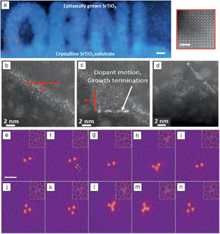
The fourth challenge refers to real-time feedback. Until now, the vast majority of atomically resolved (and mesoscopic) imaging studies have been performed using predefined rectangular scan areas, with adjustments performed based on evaluation by a human operator. For imaging systems with a small number of regions of interest, and especially for beam- or probe-induced manipulation, real-time image-based feedback is required.^{Reference Kalinin, Borisevich and Jesse41} The example of Fourier transform-based feedback for atomic fabrication has recently been introduced, as shown in Figure 9.^{Reference Dyck, Kim, Jimenez-Izal, Alexandrova, Kalinin and Jesse12,Reference Jesse, Hudak, Zarkadoula, Song, Maksov, Fuentes-Cabrera, Ganesh, Kravchenko, Snijders, Lupini, Borisevich and Kalinin42} Ultimately, we envision that such approaches can be combined with beam-induced reaction and electrocatalysis to introduce beam-powered and beam-controlled molecular actuators and machines.

Figure 9.

(a) Left: Scanning transmission electron microscope image showing text that Oak Ridge National Laboratory sculptured via electron-beam-induced crystallization of SrTiO₃. Scale bar = 5 nm. Right: Zoomed in area from the red square. Scale bar = 2 nm.^{Reference Jesse, He, Lupini, Leonard, Oxley, Ovchinnikov, Unocic, Tselev, Fuentes-Cabrera, Sumpter, Pennycook, Kalinin and Borisevich17} (b–d) Beam-induced crystallization and dopant front motion in Si, illustrating the potential for atomic-scale material and dopant engineering in commercial semiconductors. (b) Inducing crystal growth and dopant motion in [111], the result of which is shown in (c). (d) Pushing dopants deeper into the crystal. The thick red arrows show the direction of the beam slow advance. The thick red base lines illustrate the scan width.^{Reference Jesse, Hudak, Zarkadoula, Song, Maksov, Fuentes-Cabrera, Ganesh, Kravchenko, Snijders, Lupini, Borisevich and Kalinin42} (e–n) Direct electron-beam (e-beam) atom-by-atom assembly of Si clusters in graphene. Shown are sequential segments of assembly of the four-atom “fidget spinner” cluster. The arrows in (f) are pointing out the rotation of the two carbon atoms. Notice that in (h) the Si dimer obtains an additional Si atom from a Si “reservoir” outside the scan frame. The third Si atom is then knocked away by the e-beam before reattaching in a more stable configuration by substituting the two C atoms that rotated in (e–g). The insets in (e–n) show the proposed atomic structure for each observed experimental image. Scale bar = 0.5 nm.^{Reference Dyck, Kim, Jimenez-Izal, Alexandrova, Kalinin and Jesse12}

Summary

The first experimental insights into atomic structure of solids were obtained in the beginning of the 20th century, as recognized by the Nobel Prize for the Braggs in 1915. Since then, Fourier-based descriptions of structure and quasiparticles have become the primary language of condensed-matter physics. From the mid to the end of the century, the emergence of electron and probe microscopies has allowed for visualizing structures of solids with atomic resolution. Yet much of the effort has been centered on the purely instrumental aspect of this research, with relatively little effort aimed at understanding the fundamental physics and chemistry from the imaging data. Currently, advances in dynamics, low-dose imaging, and advanced sample environments allow in-depth studies of materials dynamics at the single-atom level and have opened the pathway for atomic manipulation.

These opportunities—to control materials on a single-atom level and understand the fundamental physics—provide us with a new way to address Feynman’s challenge: “What I cannot create, I do not understand.”⁴³ With the advent of local probes and local structural and chemical information, not only from electron and scanning probe, but also from tomography (e.g., atom probe), the challenges lie in determining the building blocks of the generative models that underpin the physics of the system.

Recent advances in machine learning, including generative adversarial networks, may provide a starting point for learning the important descriptors directly from available data. Combining information from diverse sources into a single framework in a self-consistent manner and using it to reinforce theory-experiment feedback loops remains an open challenge. Correctly determining the underlying physics in real time can provide in situ feedback to tailor and build structures to meet specific requirements that would otherwise be impossible without both the rapid identification (enabled by machine learning) as well as the rapid predictions enabled by integrated modeling efforts.