1. Introduction
In the classical risk model, claims occur as a Poisson process and the distribution of individual claims is fixed, meaning that in this model neither claim arrival intensities nor the individual claim amount distribution change over time. For some situations it may be more realistic to relax these assumptions and to let the arrival intensities and claim amount distribution change. This issue was addressed for the first time by Ammeter (Reference Ammeter1948). He considered a model that starts each year with a new claims intensity which is independent of past intensities. An alternative model assumes that the arrival intensities are governed by a continuous time Markov chain on a finite state space which models, for example, a changing financial environment. Discussions of risk models in a Markovian environment can be found in, for example, Reinhard (Reference Reinhard1984), Asmussen (Reference Asmussen1989), Grandell (Reference Grandell1991) and Asmussen & Albrecher (Reference Asmussen and Albrecher2010).
In this paper we study Markov-modulated risk models. In the continuous time model, the arrival intensities and the distribution of the individual claim amounts in different time intervals depend on a state process, representing, for example, different weather, economic, or environmental conditions, and therefore can be considered more flexible than the classical risk model. There is much research that considers ruin-related quantities in the framework of the continuous time Markov-modulated model. However, there are few papers that contain explicit solutions for ruin-related quantities, and these mostly relate to the case of two states. Lu & Li (Reference Lu and Li2005) find an expression for the Laplace transform of the infinite time survival probability. They invert this transform when there are two states in the cases when individual claims are exponentially distributed and when the individual claim amount distributions belong to the K n family (so that the Laplace transform of each individual claim amount density is the ratio of polynomials in the transform argument, with the degree of the denominator polynomial being higher). Lu (Reference Lu2006) expands work by Snoussi (Reference Snoussi2002) on the probability and severity of ruin. She obtains explicit solutions in the case of exponential and mixed Erlang individual claim amount distributions when there are two states. Ng & Yang (Reference Ng and Yang2006) consider the joint distribution of the surplus prior to ruin and the deficit at ruin, and obtain explicit solutions when the initial surplus is zero when individual claim amounts are phase-type distributed. Li & Lu (Reference Li and Lu2008) construct a Gerber–Shiu function and obtain explicit solutions in the case when the initial surplus is zero. Reinhard (Reference Reinhard1984) considers the finite time ruin probability and obtains formulae, but does not illustrate their application. Li et al. (Reference Li, Dickson and Li2014) also consider finite time ruin problems, give formulae for the density of the time of ruin, and consider the computational issues associated with the application of their results. Many results in the literature seem difficult to apply in the case of more than two states. For example, Lu (Reference Lu2006) derives a set of equations satisfied by the Laplace transforms of the probability and severity of ruin functions. It does not seem like a straightforward exercise to invert these, even numerically.
For the discrete time model, the main studies we build on are by Reinhard & Snoussi (Reference Reinhard and Snoussi2002) who consider the probability and severity of ruin, and by Chen et al. (Reference Chen, Yuen and Guo2014) who consider the case of two states and obtain a recursion scheme for calculating ultimate ruin probabilities, which includes equations satisfied by the ruin probabilities when the initial surplus is zero. Building on these studies, our purpose is to apply a discrete time model that can provide approximations to ruin-related quantities in a continuous time Markov-modulated risk model for which explicit solutions do not exist. Our techniques are based on numerical algorithms presented by Dickson & Waters (Reference Dickson, Egídio dos Reis and Waters1991, Reference Dickson and Waters1992); see also De Vylder & Goovaerts (Reference De Vylder and Goovaerts1988). We show how we can adapt these algorithms and find approximations to the probability of ruin in both infinite and finite time, and to the probability and severity of ruin.
This paper is organised as follows. In section 2 we present notation and state definitions. In section 3 we provide recursive formulae for the probability of ruin and the probability and severity of ruin for a discrete two-state Markov-modulated model. Then, in section 4 we show how we can apply the results in section 3 to approximate the corresponding quantities in a continuous time Markov-modulated model. Finally, in section 5 we consider the finite time ruin probability for a model with m≥2 states, and we briefly discuss how we can bound/approximate the ultimate ruin probability for such a model.
2. Models and Notation
We denote the surplus of an insurance company in continuous time by {U(t)}
t≥0 and define it as U(t)=u+ct−S(t), where
 $$S(t)\,{\equals}\mathop{\sum}\nolimits_{i\,{\equals}\,1}^{N(t)} X_{i} $$
and N(t) is the number of claims that have occurred up to time t. Let {J(t)}
t≥0 be a homogeneous, irreducible and aperiodic continuous time Markov process representing different environments in which the insurer operates (e.g. financial conditions or weather conditions). This process has a finite state space M={1, …, m}, and intensity matrix A=(α
ij
)
i,j∈M
, where α
ii
:=−α
i
, for i∈M, and π=(π
1, … , π
m
) is the unique stationary probability distribution of {J(t)}
t≥0, given by
 $$\pi _{i} \,{\equals}\,{{(\lambda _{i} \eta _{i} )/\alpha _{i} } \over {\mathop{\sum}\limits_{j\,{\equals}\,1}^m {(\lambda _{j} \eta _{j} )/\alpha _{j} } }}$$
where η i is the unique stationary probability distribution of the embedded Markov chain with transition probabilities q ii =0 and q ij =α ij /α i ; see Reinhard (Reference Reinhard1984). In this model, in the time interval (t, t+dt) claims occur according to a Poisson process with intensity λ i if J(s)=i for all s in (t, t+dt), and the corresponding claim amounts have distribution function F i and density function f i , with finite mean m i . The initial surplus is u and c is the premium income per unit of time. We assume that c is fixed regardless of the state of the environment process and satisfies the positive loading condition (see e.g. Albrecher & Boxma, Reference Albrecher and Boxma2005):
 $$\mathop{\sum}\limits_{i\,{\equals}\,1}^m {\pi _{i} m} _{j}\,\,\lt\,\,c\mathop{\sum}\limits_{i\,{\equals}\,1}^m {{\pi _{i} } \over {\lambda _{i} }}$$
Define
 $$T_{u} \,{\equals}\,{\rm inf}\{ t\:\,\colon\,\;\:U(t)\,\,\lt\,\,0\left| U \right.(0)\,{\equals}\,u\} $$
, with T
u
=∞ if U(t)≥0 for all t≥0 to be the time of ruin given initial surplus u. Then, the probability that ruin occurs in infinite time due to a claim in state j, given initial state i and initial surplus u, is defined by ψ
ij
(u)=Pr(T
u
<∞, J(T
u
)=j│U(0)=u, J(0)=i). Further, the probability that ruin occurs in infinite time given initial surplus u and initial environment state i is given by
 $$\psi _{i} (u)\,{\equals}\Pr (T_{u} \,\lt\,\infty\,\mid\,U(0)\,{\equals}\,u,J(0)\,{\equals}\,i)$$
and δ
i
(u)=1−ψ
i
(u). We denote by ψ
i
(u, t) the probability of ruin in finite time and define it by
 $$\psi _{i} (u,t){\equals}\Pr (T_{u} \leq t\,\mid\,U(0)\,{\equals}\,u,J(0)\,{\equals}\,i)$$
. Also, we define
 $$H_{{ij}} (u,y)\,{\equals}\Pr \left( {T_{u} \,\lt\,\infty\,{\rm and}\mid U\left( {T_{u} } \right)\mid\leq y,J\left( {T_{u} } \right)\,{\equals}\,j\mid U(0)\,{\equals}\,u,J(0){\equals}\,i} \right)$$
to be the probability that ruin occurs in state j and that the deficit at ruin, or the severity of ruin, is at most y, given initial state i. Then
 $$h_{{ij}} (u,y){\equals}{\partial \over {\partial y}}H_{{ij}} (u,y)$$
is its defective density, and
 $$H_{i} (u,y)\,{\equals}\,\Pr \left( {T_{u} \,\lt\,\infty\,{\rm and}\mid\,U\left( {T_{u} } \right)\mid \leq y\,\mid\,U(0)\,{\equals}\,u,J(0)\,{\equals}\,i} \right)$$
is the probability that ruin occurs and that the deficit at the time of ruin is at most y, given initial state i, and
 $$H_{i} (u,y)\,{\equals}\,\mathop{\sum}\nolimits_{j{\equals}1}^m H_{{ij}} (u,y)$$
.
We now introduce our discrete time model that can be used to approximate the continuous time Markov-modulated model. In this model, the insurer’s surplus at time n, n=1, 2, 3, … is denoted by U
d
(n) and is defined as
 $$U^{d} (n)\,{\equals}\,u{\plus}n{\minus}\mathop{\sum}\nolimits_{i\,{\equals}\,1}^n Y_{i} $$
, where u is a non-negative integer representing the insurer’s initial surplus, the premium income per unit time is 1 (so that n is the total premium income up to time n), and Y
i
denotes the insurer’s aggregate claim amount in the ith time period. Let {J
n
}
n∈N
be a homogeneous, irreducible and aperiodic Markov chain with a finite state space M={1, … , m} and transition probabilities
 $$p_{{ij}} \,{\equals}\,{\rm Pr}\left( {J_{n} {\equals}\,j \mid J_{{n{\minus}1}} \,{\equals}\,i,J_{k} \,{\rm for}\,k\leq n{\minus}1} \right)$$
, for i, j∈M. The conditional joint distribution of Y
n
and J
n
given the previous state J
n−1 is defined by
 $$g_{{ij}} (x)\,{\equals}\,{\rm Pr}\left( {Y_{n} \,{\equals}\,x,J_{n} \,{\equals} j \mid J_{{n{\minus}1}} \,{\equals}\,i,\left\{ {J_{k} ,Y_{k} } \right\},\,{\rm for}\,k\leq n{\minus}1} \right)\,{\equals}\,p_{{ij}} g_{j} (x)$$
for x=0, 1, 2, … , where
 $$\mathop{\sum}\nolimits_{x\,{\equals}\,0}^\infty g_{{ij}} (x)\,{\equals}\,p_{{ij}} $$
, with
 $$g_{i} (x){\equals}\mathop{\sum}\nolimits_{j\,{\equals}\,1}^m g_{{ij}} (x)$$
, and
 $$G_{i} (y)\,{\equals}\,\mathop{\sum}\nolimits_{j\,{\equals}\,1}^m \mathop{\sum}\nolimits_{x\,{\equals}\,0}^y g_{{ij}} (x)$$
for y=0, 1, 2, …. Further,
 $$\tilde{g}_{{ij}} (s)\,{\equals}\mathop{\sum}\nolimits_{x\,{\equals}\,0}^\infty s^{x} g_{{ij}} (x)$$
. For all i, j∈M and n=1, 2, 3, … , we define
 $$\mu _{{ij}} \,{\equals}\mathop{\sum}\nolimits_{x\,{\equals}\,1}^\infty xg_{{ij}} (x)$$
and
 $$\mu _{i} \,{\equals}\mathop{\sum}\nolimits_{j{\equals}1}^m \mu _{{ij}} $$
. We assume that the net profit condition holds, namely
 $$\mathop{\sum}\nolimits_{j\,{\equals}\,1}^m \tilde{\pi }_{j} \:\mu _{j} \,\lt\,1$$
, where
 $$\{ \tilde{\pi }_{j} \} _{{j\,{\equals}\,1}}^{m} $$
is the unique stationary distribution of
 $$\{ p_{{ij}} \} _{{i,j\,{\equals}\,1}}^{m} $$
.
Let
 $$T_{u}^{d} \,{\equals}\,min\{ n\geq 1\,\colon\,U^{d} (n)\leq 0 \mid U^{d} (0)\,{\equals}\,u\} $$
denote the time of ruin given initial surplus u, with
 $$T_{u}^{d} \,{\equals}\,\infty$$
if U
d
(n)>0 for n=1, 2, 3, …. We remark that as our aim in this paper is to approximate the continuous time Markov-modulated model we assume that ruin occurs when the surplus falls to zero or below zero in line with Dickson & Waters (Reference Dickson, Egídio dos Reis and Waters1991, Reference Dickson and Waters1992) who found that such a definition gives a better approximation to ruin probabilities in the classical risk model (which is a special case of the continuous time Markov-modulated risk model). This contrasts with Chen et al. (Reference Chen, Yuen and Guo2014) who assumed that ruin occurs on the first occasion that the surplus is strictly negative.
Denote by
 $$\psi _{i}^{d} (u)$$
the ultimate probability of ruin given initial surplus u and initial environment state i which is given by
 $$\psi _{i}^{d} (u)\,{\equals}\,{\rm Pr}(T_{u}^{d} \,\lt\,\infty \mid U^{d} (0)\,{\equals}\,u,J_{0} \,{\equals}\,i)\,{\equals}\,1{\minus}\delta _{i}^{d} (u)$$
where
 $$\delta _{i}^{d} (u)$$
is the probability of survival. Also, we denote by
 $$\psi _{i}^{d} (u,t)$$
the finite time probability of ruin given initial surplus u and initial environment state i which is given by
 $$\psi _{i}^{d} (u,t)\,{\equals}\,{\rm Pr}(T_{u}^{d} \leq t \mid U^{d} (0)\,{\equals}\,u,J_{0} \,{\equals}\,i)$$
. Further, we define the probability that ruin occurs in state j and the insurer’s deficit at ruin is at most y, given initial environment state i, as
 $$H_{{ij}}^{d} (u,y)\,{\equals}\,{\rm Pr}(T_{u}^{d} \,\lt\,\infty, \mid U(T_{u}^{d} ) \mid \lt\,y,J_{{T_{u}^{d} }} \,{\equals}\,j \mid U^{d} (0)\,{\equals}\,u,J_{0} \,{\equals}\,i)$$
with the probability mass function being
 $$h_{{ij}}^{d} (u,y)$$
, and let
 $$h_{i}^{d} (u,y){\equals}\mathop{\sum}\nolimits_{j\,{\equals}\,1}^m h_{{ij}}^{d} (u,y)$$
. Further,
 $$H_{i}^{d} (u,y){\equals}\mathop{\sum}\nolimits_{j\,{\equals}\,1}^m H_{{ij}}^{d} (u,y)$$
.
3. The Probability of Ruin and the Probability and Severity of Ruin
In this section, we consider the discrete time model and present recursive formulae for
 $$\psi _{i}^{d} (u)$$
and
 $$h_{i}^{d} (u,y)$$
when m=2. As our recursive formulae need initial values, we first give expressions for
 $$\psi _{i}^{d} (0)$$
and
 $$h_{i}^{d} (0,y)$$
, and then provide results which we can use to calculate the ultimate ruin probability and the probability and severity of ruin.
3.1. Initial values
 $$\bipsi _{\mib i}^{\mib d} (\bf 0)$$
and
$${\mib h}_{{\mib ij}}^{\mib d} (\mib {\rm \bf 0},{y})$$


Chen et al. (Reference Chen, Yuen and Guo2014) derived two equations that define the relationship between
 $$\delta _{1}^{d} (0)$$
and
 $$\delta _{2}^{d} (0)$$
under their definition of ruin. Here, we develop the equivalent of their equations for our definition of ruin. The first equation ((3.1) below) is obtained by a different approach, but for the second equation ((3.2) below) we can use the method of generating functions as in Chen et al. (Reference Chen, Yuen and Guo2014).
Theorem 3.1
When m=2,
 $$\delta _{1}^{d} (0)$$
and
 $$\delta _{2}^{d} (0)$$
satisfy
 $$p_{{12}} \:\delta _{2}^{d} (0){\plus}p_{{21}} \:\delta _{1}^{d} (0)\,{\equals}\,p_{{12}} (1{\minus}\mu _{2} ){\plus}p_{{21}} (1{\minus}\mu _{1} )$$
and
 $$\left( {\tilde{g}_{{11}} (\rho )(\tilde{g}_{{22}} (\rho ){\minus}\rho ){\minus}\tilde{g}_{{12}} (\rho )\tilde{g}_{{21}} (\rho )} \right)\delta _{1}^{d} (0)\,{\equals}\,\left( {\tilde{g}_{{12}} (\rho )\tilde{g}_{{22}} (\rho ){\minus}\tilde{g}_{{12}} (\rho )(\tilde{g}_{{22}} (\rho ){\minus}\rho )} \right)\delta _{2}^{d} (0)$$
where ρ∈(0, 1) is the solution to
 $$L_{1} (s)\,{\equals}\,\left( {\tilde{g}_{{11}} (s){\minus}s} \right)\left( {\tilde{g}_{{22}} (s){\minus}s} \right){\minus}\tilde{g}_{{12}} (s)\tilde{g}_{{21}} (s)\,{\equals}\,0$$
We remark that the existence of ρ is shown by Chen et al. (Reference Chen, Yuen and Guo2014).
Proof: By considering what can happen in the first time period we have
 $$\psi _{i}^{d} (u)\,{\equals}\,\mathop{\sum}\limits_{j\,{\equals}\,1}^2 \mathop{\sum}\limits_{x\,{\equals}\,0}^u g_{{ij}} (x)\psi _{j}^{d} (u{\plus}1{\minus}x){\plus}\mathop{\sum}\limits_{j\,{\equals}\,1}^2 \mathop{\sum}\limits_{x\,{\equals}\,u{\plus}1}^\infty g_{{ij}} (x)$$
We now assume that
 $$\mathop{\sum}\nolimits_{u\,{\equals}\,0}^\infty \psi _{i}^{d} (u)\,\lt\,\infty$$
, and we discuss conditions under which this assumption holds in the Appendix.
Summing over u from 0 to ∞ in (3.4) and changing the order of summations on the right-hand side we obtain
 $$\psi _{1}^{d} (0){\plus}\mathop{\sum}\limits_{u\,{\equals}\,1}^\infty \psi _{1}^{d} (u)\,{\equals}\,p_{{11}} \mathop{\sum}\limits_{u\,{\equals}\,1}^\infty \psi _{1}^{d} (u){\plus}\mu _{{11}} {\plus}p_{{12}} \mathop{\sum}\limits_{u\,{\equals}\,1}^\infty \psi _{2}^{d} (u){\plus}\mu _{{12}} $$
and
 $$\psi _{2}^{d} (0){\plus}\mathop{\sum}\limits_{u\,{\equals}\,1}^\infty \psi _{2}^{d} (u)\,{\equals}\,p_{{21}} \mathop{\sum}\limits_{u\,{\equals}\,1}^\infty \psi _{1}^{d} (u){\plus}\mu _{{21}} {\plus}p_{{22}} \mathop{\sum}\limits_{u\,{\equals}\,1}^\infty \psi _{2}^{d} (u){\plus}\mu _{{22}} $$
Rearranging, formula (3.1) follows.
We can build the second relationship between
 $$\delta _{1}^{d} (0)$$
and
 $$\delta _{2}^{d} (0)$$
using the method of generating functions used by Chen et al. (Reference Chen, Yuen and Guo2014). As the techniques are very similar, we omit the details.
The next result gives the initial values
 $$h_{{ij}}^{d} (0,y)$$
. This result holds under the assumptions
A1. p 22 p 11>p 12 p 21, and
A2.
 $$p_{{21}} \:A_{{11}} (1,\,y){\plus}p_{{12}} \:A_{{21}} \left( {1,\,y} \right)\,\lt\,p_{{21}} \:h_{{11}}^{d} (0,\,y){\plus}p_{{12}} \:h_{{21}}^{d} (0,\,y)$$
, where we define
Aij
(s, y)=
 $$\mathop{\sum}\limits_{u\,{\equals}\,0}^\infty s^{{u{\plus}1}} g_{{ij}} (u{\plus}1{\plus}y)$$
.
We comment on these assumptions after the proof of Theorem 3.2.
Theorem 3.2
When m=2, for y=0, 1, 2, … ,
 $$h_{{11}}^{d} (0,\,y)$$
and
 $$h_{{21}}^{d} (0,\,y)$$
satisfy
 $$p_{{12}} h_{{21}}^{d} (0,\,y){\plus}p_{{21}} h_{{11}}^{d} (0,\,y)\,{\equals}\,p_{{12}} \left( {p_{{21}} {\minus}G_{{21}} (y)} \right){\plus}p_{{21}} \left( {p_{{11}} {\minus}G_{{11}} (y)} \right)$$
and
 $$\eqalignno{ & \quad h_{{11}}^{d} (0,\,y)\left( {\tilde{g}_{{11}} (\rho )\left( {\tilde{g}_{{22}} (\rho ){\minus}\rho } \right){\minus}\tilde{g}_{{12}} (\rho )\tilde{g}_{{21}} (\rho )} \right){\plus}\tilde{g}_{{12}} (\rho )\:A_{{21}} (\rho ,\,y) \cr & {\equals}\,h_{{21}}^{d} (0,\,y)\left( {\tilde{g}_{{12}} (\rho )\tilde{g}_{{22}} (\rho ){\minus}\tilde{g}_{{12}} (\rho )\left( {\tilde{g}_{{22}} (\rho ){\minus}\rho } \right)} \right){\plus}\left( {\tilde{g}_{{22}} (\rho ){\minus}\rho } \right)A_{{11}} (\rho ,\,y) $$
Further,
 $$h_{{22}}^{d} (0,\,y)$$
and
 $$h_{{12}}^{d} (0,\,y)$$
satisfy
 $$p_{{12}} h_{{22}}^{d} (0,\,y){\plus}p_{{21}} h_{{12}}^{d} (0,\,y)\,{\equals}\,p_{{12}} \left( {p_{{22}} {\minus}G_{{22}} (y)} \right){\plus}p_{{21}} \left( {p_{{12}} {\minus}G_{{12}} (y)} \right)$$
and
 $$\eqalignno{ & \quad h_{{12}}^{d} (0,\,y)\left( {\tilde{g}_{{11}} (\rho )\left( {\tilde{g}_{{22}} (\rho ){\minus}\rho } \right){\minus}\tilde{g}_{{12}} (\rho )\tilde{g}_{{21}} (\rho )} \right){\plus}\tilde{g}_{{12}} (\rho )\:A_{{22}} (\rho ,\,y) \cr & {\equals}\,h_{{22}}^{d} (0,\,y)\left( {\tilde{g}_{{12}} (\rho )\tilde{g}_{{22}} (\rho ){\minus}\tilde{g}_{{12}} (\rho )\left( {\tilde{g}_{{22}} (\rho ){\minus}\rho } \right)} \right){\plus}\left( {\tilde{g}_{{22}} (\rho ){\minus}\rho } \right)A_{{12}} (\rho ,\,y) $$
where ρ is the solution to equation (3.3).
Proof: We adapt ideas in Reinhard & Snoussi (Reference Reinhard and Snoussi2002) to our definition of ruin and write
 $$h_{{ij}}^{d} (u,\,y){\equals}\mathop{\sum}\limits_{l{\equals}1}^2 \mathop{\sum}\limits_{x{\equals}0}^u g_{{il}} (x)h_{{lj}}^{d} (u{\plus}1{\minus}x,\,y){\plus}g_{{ij}} (u{\plus}1{\plus}y)$$
Assuming
 $$\mathop{\sum}\nolimits_{u\,{\equals}\,0}^\infty h_{{ij}}^{d} (u,\,y)\,\lt\,\infty$$
(which holds if
 $$\mathop{\sum}\nolimits_{u\,{\equals}\,0}^\infty \psi _{i}^{d} (u)\,\lt\,\infty$$
), summing over u then changing the order of summation on the right-hand side and solving a system of equations, yields formulae (3.7) and (3.9).
We next apply the method of generating functions used by Chen et al. (Reference Chen, Yuen and Guo2014) to build the second pair of equations. Multiplying formula (3.11) by s u+1 and summing over u yields:
 $$\mathop{\sum}\limits_{u\,{\equals}\,0}^\infty s^{{u{\plus}1}} h_{{ij}}^{d} (u,\,y)\,{\equals}\mathop{\sum}\limits_{l\,{\equals}\,1}^2 \mathop{\sum}\limits_{u\,{\equals}\,0}^\infty \mathop{\sum}\limits_{x\,{\equals}\,0}^u s^{{u{\plus}1}} g_{{il}} (x)h_{{lj}}^{d} (u{\plus}1{\minus}x,y){\plus}\mathop{\sum}\limits_{u\,{\equals}\,0}^\infty s^{{u{\plus}1}} g_{{ij}} (u{\plus}1{\plus}y)$$
We define
 $$\tilde{h}_{{ij}}^{d} (s,\,y)\,{\equals}\mathop{\sum}\nolimits_{u\,{\equals}\,0}^\infty s^{u} h_{{ij}}^{d} (u,\,y)$$
, and set n=u+1 in the first term on the right-hand side of (3.12) to get
 $$s\tilde{h}_{{ij}}^{d} (s,y)\,{\equals}\mathop{\sum}\limits_{l\,{\equals}\,1}^2 \mathop{\sum}\limits_{n\,{\equals}\,1}^\infty \mathop{\sum}\limits_{x\,{\equals}\,0}^{n{\minus}1} s^{n} g_{{il}} (x)h_{{lj}}^{d} (n{\minus}x,\,y){\plus}A_{{ij}} (s,\,y)$$
Hence
 $$s\tilde{h}_{{ij}}^{d} (s,\,y)\,{\equals}\mathop{\sum}\limits_{l\,{\equals}\,1}^2 \tilde{g}_{{il}} (s)\tilde{h}_{{lj}}^{d} (s,\,y){\minus}e_{{ij}} (s,\,y){\plus}A_{{ij}} (s,\,y)$$
where
 $$e_{{ij}} (s,\,y)\,{\equals}\,\mathop{\sum}\nolimits_{l\,{\equals}\,1}^2 \tilde{g}_{{il}} (s)h_{{lj}}^{d} (0,\,y)$$
. We can write (3.13) for i=1, 2 and j=1 as
 $$\left\{ {\matrix{ {(\tilde{g}_{{11}} (s){\minus}s)\tilde{h}_{{11}}^{d} (s,\,y){\plus}\tilde{g}_{{12}} (s)\tilde{h}_{{21}}^{d} (s,\,y)\,{\equals}\,e_{{11}} (s,\,y){\minus}A_{{11}} (s,\,y)} \cr {\tilde{g}_{{21}} (s)\tilde{h}_{{11}}^{d} (s,\,y){\plus}(\tilde{g}_{{22}} (s){\minus}s)\tilde{h}_{{21}}^{d} (s,\,y)\,{\equals}\,e_{{21}} (s,\,y){\minus}A_{{21}} (s,\,y)} \cr } } \right.$$
giving
 $$\eqalignno{ & \left( {\left( {\tilde{g}_{{11}} (s){\minus}s} \right)\left( {\tilde{g}_{{22}} (s){\minus}s} \right){\minus}\tilde{g}_{{12}} (s)\tilde{g}_{{21}} (s)} \right)\tilde{h}_{{11}}^{d} (s,\,y) \cr & {\equals}\,\left( {\tilde{g}_{{22}} (s){\minus}s} \right)e_{{11}} (s,\,y){\minus}\tilde{g}_{{12}} (s)e_{{21}} (s,\,y){\plus}\tilde{g}_{{12}} (s)A_{{21}} (s,\,y){\minus}\left( {\tilde{g}_{{22}} (s){\minus}s} \right)A_{{11}} (s,\,y) $$
Similarly, for i=1, 2 and j=2 we have
 $$\left\{ {\matrix{ {(\tilde{g}_{{11}} (s){\minus}s)\tilde{h}_{{12}}^{d} (s,\,y){\plus}\tilde{g}_{{12}} (s)\tilde{h}_{{22}}^{d} (s,\,y)\,{\equals}\,e_{{12}} (s,\,y){\minus}A_{{12}} (s,\,y)} \cr {\tilde{g}_{{21}} (s)\tilde{h}_{{12}}^{d} (s,\,y){\plus}(\tilde{g}_{{22}} (s){\minus}s)\tilde{h}_{{22}}^{d} (s,\,y)\,{\equals}\,e_{{22}} (s,\,y){\minus}A_{{22}} (s,\,y)} \cr } } \right.$$
giving
 $$\eqalignno{ & \quad \left( {\left( {\tilde{g}_{{11}} (s){\minus}s} \right)\left( {\tilde{g}_{{22}} (s){\minus}s} \right){\minus}\tilde{g}_{{12}} (s)\tilde{g}_{{21}} (s)} \right)\tilde{h}_{{12}}^{d} (s,y) \cr & {\equals}\,\left( {\tilde{g}_{{22}} (s){\minus}s} \right)e_{{12}} \left( {s,y} \right){\minus}\tilde{g}_{{12}} (s)e_{{22}} (s,y){\plus}\tilde{g}_{{12}} (s)A_{{22}} (s,y){\minus}\left( {\tilde{g}_{{22}} (s){\minus}s} \right)A_{{12}} (s,y) $$
Inserting for e
11(s, y) and e
21(s, y), we can write equation (3.14) as
 $$L_{1} (s)\tilde{h}_{{11}}^{d} (s,y)\,{\equals}\,L_{2}^{{(1)}} (s,y)$$
, where L
1(s) is given by (3.3), and
 $$\eqalignno{ L_{2}^{{(1)}} (s,y)\,{\equals}\, & \left( {\left( {\tilde{g}_{{22}} (s){\minus}s} \right)\tilde{g}_{{11}} (s){\minus}\tilde{g}_{{12}} (s)\tilde{g}_{{21}} (s)} \right)h_{{11}}^{d} (0,y){\plus}\tilde{g}_{{12}} (s)A_{{21}} (s,y) \cr & {\plus}\left( {\left( {\tilde{g}_{{22}} (s){\minus}s} \right)\tilde{g}_{{12}} (s){\minus}\tilde{g}_{{12}} (s)\tilde{g}_{{22}} (s)} \right)h_{{21}}^{d} \left( {0,y} \right){\minus}\left( {\tilde{g}_{{22}} (s){\minus}s} \right)A_{{11}} (s,y) $$
Similarly, equation (3.15) can be written as
 $$L_{1} (s)\tilde{h}_{{12}}^{d} (s,y)\,{\equals}\,L_{2}^{{(2)}} \left( {s,y} \right)$$
, where
 $$\eqalignno{ L_{2}^{{(2)}} \left( {s,y} \right)\,{\equals}\, & \left( {\left( {\tilde{g}_{{22}} (s){\minus}s} \right)\tilde{g}_{{11}} (s){\minus}\tilde{g}_{{12}} (s)\tilde{g}_{{21}} (s)} \right)h_{{12}}^{d} (0,y){\plus}\tilde{g}_{{12}} (s)A_{{22}} \left( {s,y} \right) \cr & {\plus}\left( {\left( {\tilde{g}_{{22}} (s){\minus}s} \right)\tilde{g}_{{12}} (s){\minus}\tilde{g}_{{12}} (s)\tilde{g}_{{22}} (s)} \right)h_{{22}}^{d} (0,y){\minus}\left( {\tilde{g}_{{22}} (s){\minus}s} \right)A_{{12}} (s,y) $$
Setting s=0 in equation (3.16), and noting that A ij (0, y)=0, we have
 $$L_{2}^{{(1)}} (0,y)\,{\equals}\,\left( {g_{{22}} (0)g_{{11}} (0){\minus}g_{{12}} (0)g_{{21}} (0)} \right)h_{{11}}^{d} (0,y)$$
Also, setting s=1 in equation (3.16) gives
 $$L_{2}^{{(1)}} (1,y)\,{\equals}\,{\minus}p_{{21}} \:h_{{11}}^{d} (0,y){\plus}p_{{12}} A_{{21}} (1,y){\minus}p_{{12}} \:h_{{21}}^{d} (0,y){\plus}p_{{21}} A_{{11}} (1,y)$$
We note that
 $$L_{2}^{{(1)}} (0,y)\,\gt\,0$$
under assumption A1, and
 $$L_{2}^{{(1)}} (1,y)\,\lt\,0$$
under assumption A2. So we can conclude that there exists ρ∈(0, 1) such that
 $$L_{1} (\rho ){\equals}L_{2}^{{(1)}} (\rho ,y){\equals}0$$
, and by the same argument that
 $$L_{1} (\rho ){\equals}L_{2}^{{(2)}} (\rho ,y){\equals}0$$
. Therefore, we can find the second pair of equations that defines the relationship between h
11(0, y), h
21(0, y) and h
12(0, y), h
22(0, y).
We cannot give any intuitive explanations of assumptions A1 and A2. In our application of the results in Theorem 3.2, we will choose parameters such that the probability of a change of state is very small regardless of the initial state, meaning that A1 will easily be satisfied. We found that A2 was always satisfied under our parameter choices. We remark that this assumption suggests that there is not a simple extension of formula (3.5) in Dickson & Waters (Reference Dickson and Waters1992).
We remark that the approach of Chen et al. (Reference Chen, Yuen and Guo2014) can be used to obtain equation (3.7). This approach does not require the assumption
 $$\mathop{\sum}\nolimits_{u\,{\equals}\,0}^\infty h_{{ij}}^{d} \left( {u,y} \right)\,\lt\,\infty$$
, but the proof is longer.
3.2. The probability of ultimate ruin
Chen et al. (Reference Chen, Yuen and Guo2014) developed recursive formulae for the probability of ultimate ruin in their discrete time model with m=2. Using exactly the same ideas, but with our definition of ruin, our result that corresponds to equation (3) of Chen et al. (Reference Chen, Yuen and Guo2014) is
 $$\psi _{i}^{d} (u)\,{\equals}\,\mathop{\sum}\limits_{j\,{\equals}\,1}^2 \mathop{\sum}\limits_{x\,{\equals}\,0}^u g_{{ij}} (x)\psi _{j}^{d} (u{\plus}1{\minus}x){\plus}\mathop{\sum}\limits_{j\,{\equals}\,1}^2 \mathop{\sum}\limits_{x\,{\equals}\,u{\plus}1}^\infty g_{{ij}} (x)$$
for i=1, 2. Proceeding with this formula, we have encountered the problem of numerical instability. This problem arises because the application of these two formulae involves subtracting many terms, which is a reason for a recursion scheme to be unstable. See Panjer & Wang (Reference Panjer and Wang1993) for a discussion of this issue in the case m=1. To address this problem, we apply ideas from Dickson et al. (Reference Dickson and Waters1995) to obtain the following result.
Theorem 3.3 When m=2, for u=1, 2, 3, … , we have
 $$\eqalignno{ \psi _{1}^{d} (u)\,{\equals}\, & f^{{{\minus}1}} \left( {\left( {1{\minus}h_{{22}}^{d} \left( {0,0} \right)} \right)\psi _{1}^{d} (0){\plus}h_{{12}}^{d} \left( {0,0} \right)\psi _{2}^{d} (0)} \right. \cr & {\plus}\mathop{\sum}\limits_{x\,{\equals}\,1}^{u{\minus}1} \psi _{1}^{d} \left( {u{\minus}x} \right)\left( {\left( {1{\minus}h_{{22}}^{d} \left( {0,0} \right)} \right)h_{{11}}^{d} \left( {0,x} \right){\plus}h_{{12}}^{d} \left( {0,0} \right)h_{{21}}^{d} \left( {0,x} \right)} \right) \cr & {\plus}\mathop{\sum}\limits_{x\,{\equals}\,1}^{u{\minus}1} \psi _{2}^{d} (u{\minus}x)\left( {\left( {1{\minus}h_{{22}}^{d} \left( {0,0} \right)} \right)h_{{12}}^{d} \left( {0,x} \right){\plus}h_{{12}}^{d} \left( {0,0} \right)h_{{22}}^{d} \left( {0,x} \right)} \right) \cr & \left. {{\minus}\left( {1{\minus}h_{{22}}^{d} \left( {0,0} \right)} \right)\mathop{\sum}\limits_{x{\equals}0}^{u{\minus}1} h_{1}^{d} (0,x){\minus}h_{{12}}^{d} \left( {0,0} \right)\mathop{\sum}\limits_{x\,{\equals}\,0}^{u{\minus}1} h_{2}^{d} \left( {0,x} \right)} \right) $$
and
 $$\eqalignno{ \psi _{2}^{d} (u)\,{\equals}\, & f^{{{\minus}1}} \left( {\left( {1{\minus}h_{{11}}^{d} \left( {0,0} \right)} \right)\psi _{2}^{d} (0){\plus}h_{{21}}^{d} \left( {0,0} \right)\psi _{1}^{d} (0)} \right. \cr & {\plus}\mathop{\sum}\limits_{x{\equals}1}^{u{\minus}1} \psi _{1}^{d} \left( {u{\minus}x} \right)\left( {\left( {1{\minus}h_{{11}}^{d} \left( {0,0} \right)} \right)h_{{21}}^{d} \left( {0,x} \right){\plus}h_{{21}}^{d} \left( {0,0} \right)h_{{11}}^{d} \left( {0,x} \right)} \right) \cr & {\plus}\mathop{\sum}\limits_{x\,{\equals}\,1}^{u{\minus}1} \psi _{2}^{d} \left( {u{\minus}x} \right)\left( {\left( {1{\minus}h_{{11}}^{d} \left( {0,0} \right)} \right)h_{{22}}^{d} \left( {0,x} \right){\plus}h_{{21}}^{d} \left( {0,0} \right)h_{{12}}^{d} \left( {0,x} \right)} \right) \cr & \left. {{\minus}\left( {1{\minus}h_{{11}}^{d} \left( {0,0} \right)} \right)\mathop{\sum}\limits_{x\,{\equals}\,0}^{u{\minus}1} h_{2}^{d} \left( {0,x} \right){\minus}h_{{21}}^{d} \left( {0,0} \right)\mathop{\sum}\limits_{x\,{\equals}\,0}^{u{\minus}1} h_{1}^{d} \left( {0,x} \right)} \right) $$
where
 $$f\,{\equals}\,\left( {1{\minus}h_{{11}}^{d} \left( {0,0} \right)} \right)\left( {1{\minus}h_{{22}}^{d} \left( {0,0} \right)} \right){\minus}h_{{12}}^{d} \left( {0,0} \right)h_{{21}}^{d} \left( {0,0} \right)$$
.
Proof: By considering the amount of the first drop below u (should such a drop take place) and whether or not it is accompanied by a change of environment state, we have
 $$\psi _{i}^{d} (u)\,{\equals}\,\mathop{\sum}\limits_{j\,{\equals}\,1}^2 \mathop{\sum}\limits_{x\,{\equals}\,0}^{u{\minus}1} h_{{ij}}^{d} (0,x)\psi _{j}^{d} (u{\minus}x){\plus}\mathop{\sum}\limits_{j\,{\equals}\,1}^2 \mathop{\sum}\limits_{x\,{\equals}\,u}^\infty h_{{ij}}^{d} (0,x)$$
We remark that we include 0 as a possible drop amount as this is consistent with our definition of ruin. By noting that
 $$\psi _{i}^{d} (0)\,{\equals}\mathop{\sum}\nolimits_{x\,{\equals}\,0}^\infty h_{i}^{d} \left( {0,x} \right)$$
, we can write
 $$\eqalignno{ \psi _{1}^{d} (u)\,{\equals}\, & h_{{11}}^{d} \left( {0,0} \right)\psi _{1}^{d} (u){\plus}h_{{12}}^{d} \left( {0,0} \right)\psi _{2}^{d} (u){\plus}\mathop{\sum}\limits_{x\,{\equals}\,1}^{u{\minus}1} h_{{11}}^{d} \left( {0,x} \right)\psi _{1}^{d} \left( {u{\minus}x} \right) \cr & {\plus}\mathop{\sum}\limits_{x\,{\equals}\,1}^{u{\minus}1} h_{{12}}^{d} \left( {0,x} \right)\psi _{2}^{d} \left( {u{\minus}x} \right){\plus}\psi _{1} (0){\minus}\mathop{\sum}\limits_{x\,{\equals}\,0}^{u{\minus}1} h_{1}^{d} \left( {0,x} \right) $$
with a similar equation for
 $$\psi _{2}^{d} (u)$$
. Rearranging and solving this pair of equations gives the result.
We have not experienced any numerical instability with formulae (3.18) and (3.19) as discussed by Dickson et al. (Reference Dickson and Waters1995) for the approximation of the classical risk model. These formulae can be applied provided that we know the values of
 $$\psi _{i}^{d} (0)$$
and
 $$h_{{ij}}^{d} (0,0)$$
for i, j=1, 2.
Unfortunately, we were unable to find formulae for the ultimate ruin probability when m>2. This issue arises because we need m equations to find the initial values for an m-state model. In section 5.2, we suggest a method that gives us a bound/approximation for the ultimate ruin probability for a model with m>2 states.
3.3. The probability and severity of ruin
We now derive recursive formulae for the probability and severity of ruin function in our discrete time model with m=2. For this, we adapt the ideas underlying equation (4.2) of Dickson et al. (Reference Dickson and Waters1995), which was used to approximate the probability and severity of ruin function in the classical risk model. The next theorem gives expressions for the probability and severity of ruin function in our discrete time model, from which we can approximate H i (u, y) in the continuous time Markov-modulated risk model.
Theorem 3.4 When m=2, for u=1, 2, 3, … and y=0, 1, 2, … we have
 $$\eqalignno{ H_{1}^{d} (u,y)\,{\equals}\, & f^{{{\minus}1}} \left( {\left( {1{\minus}h_{{22}}^{d} \left( {0,0} \right)} \right)\left( {H_{1}^{d} \left( {0,u{\plus}y} \right){\minus}H_{1}^{d} \left( {0,u} \right)} \right)} \right. \cr & {\plus}h_{{12}}^{d} \left( {0,0} \right)\left( {H_{2}^{d} \left( {0,u{\plus}y} \right){\minus}H_{2}^{d} \left( {0,u} \right)} \right) \cr & {\plus}\mathop{\sum}\limits_{x\,{\equals}\,1}^{u{\minus}1} H_{1}^{d} \left( {u{\minus}x,y} \right)\left( {h_{{11}}^{d} \left( {0,x} \right)\left( {1{\minus}h_{{22}}^{d} \left( {0,0} \right)} \right){\plus}h_{{12}}^{d} \left( {0,0} \right)h_{{21}}^{d} \left( {0,x} \right)} \right) \cr & \left. {{\plus}\mathop{\sum}\limits_{x\,{\equals}\,1}^{u{\minus}1} H_{2}^{d} \left( {u{\minus}x,y} \right)\left( {h_{{12}}^{d} \left( {0,x} \right)\left( {1{\minus}h_{{22}}^{d} \left( {0,0} \right)} \right){\plus}h_{{12}}^{d} \left( {0,0} \right)h_{{22}}^{d} \left( {0,x} \right)} \right)} \right) $$
and
 $$\eqalignno{ H_{2}^{d} \left( {u,y} \right)\,{\equals}\, & f^{{{\minus}1}} \left( {h_{{21}}^{d} \left( {0,0} \right)\left( {H_{1}^{d} \left( {0,u{\plus}y} \right){\minus}H_{1}^{d} \left( {0,u} \right)} \right)} \right. \cr & {\plus}\left( {1{\minus}h_{{11}}^{d} \left( {0,0} \right)} \right)\left( {H_{2}^{d} \left( {0,u{\plus}y} \right){\minus}H_{2}^{d} \left( {0,u} \right)} \right) \cr & {\plus}\mathop{\sum}\limits_{x\,{\equals}\,1}^{u{\minus}1} H_{1}^{d} \left( {u{\minus}x,y} \right)\left( {\left( {1{\minus}h_{{11}}^{d} \left( {0,0} \right)} \right)h_{{21}}^{d} \left( {0,x} \right){\plus}h_{{21}}^{d} \left( {0,0} \right)h_{{11}}^{d} \left( {0,x} \right)} \right) \cr & \left. {{\plus}\mathop{\sum}\limits_{x\,{\equals}\,1}^{u{\minus}1} H_{2}^{d} \left( {u{\minus}x,y} \right)\left( {\left( {1{\minus}h_{{11}}^{d} \left( {0,0} \right)} \right)h_{{22}}^{d} \left( {0,x} \right){\plus}h_{{21}}^{d} \left( {0,0} \right)h_{{12}}^{d} 0,x} \right)} \right) $$
where
 $$f\,{\equals}\,\left( {1{\minus}h_{{11}}^{d} \left( {0,0} \right)} \right)\left( {1{\minus}h_{{22}}^{d} \left( {0,0} \right)} \right){\minus}h_{{12}}^{d} \left( {0,0} \right)h_{{21}}^{d} \left( {0,0} \right)$$
.
Proof: Using the same approach as in the proof of the previous theorem, we obtain
 $$\eqalignno{ H_{i}^{d} \left( {u,y} \right)\,{\equals}\, & \mathop{\sum}\limits_{j\,{\equals}\,1}^2 \mathop{\sum}\limits_{x\,{\equals}\,0}^{u{\minus}1} h_{{ij}}^{d} \left( {0,x} \right)H_{j}^{d} \left( {u{\minus}x,y} \right){\plus}\mathop{\sum}\limits_{j\,{\equals}\,1}^2 \mathop{\sum}\limits_{x\,{\equals}\,u}^{u{\plus}y{\minus}1} h_{{ij}}^{d} \left( {0,x} \right) \cr & {\equals}\,H_{i}^{d} \left( {0,u{\plus}y} \right){\minus}H_{i}^{d} \left( {0,u} \right){\plus}\mathop{\sum}\limits_{j\,{\equals}\,1}^2 \mathop{\sum}\limits_{x\,{\equals}\,0}^{u{\minus}1} h_{{ij}}^{d} \left( {0,x} \right)H_{j}^{d} \left( {u{\minus}x,y} \right) $$
Noting that
 $$H_{i}^{d} \left( {0,y} \right)\,{\equals}\mathop{\sum}\limits_{x\,{\equals}\,0}^{y{\minus}1} h_{i}^{d} \left( {0,x} \right)$$
, we have
 $$\eqalignno{ H_{1}^{d} \left( {u,y} \right)\,{\equals}\, & H_{1}^{d} \left( {0,u{\plus}y} \right){\minus}H_{1}^{d} \left( {0,u} \right){\plus}h_{{11}}^{d} \left( {0,0} \right)H_{1}^{d} \left( {u,y} \right){\plus}h_{{12}} \left( {0,0} \right)H_{2}^{d} \left( {u,y} \right) \cr & {\plus}\mathop{\sum}\limits_{x\,{\equals}\,1}^{u{\minus}1} h_{{11}}^{d} \left( {0,x} \right)H_{1}^{d} \left( {u{\minus}x,y} \right){\plus}\mathop{\sum}\limits_{x\,{\equals}\,1}^{u{\minus}1} h_{{12}}^{d} \left( {0,x} \right)H_{2}^{d} \left( {u{\minus}x,y} \right) $$
with a similar equation for
 $$H_{2}^{d} \left( {u,y} \right)$$
. Rearranging and solving this pair of equations gives equations (3.20) and (3.21).
In the next section, we apply these algorithms to approximate the ultimate ruin probability and the probability and severity of ruin in the continuous time Markov-modulated model.
4. Numerical Illustrations
We now adapt the ideas of Dickson & Waters (Reference Dickson, Egídio dos Reis and Waters1991, Reference Dickson and Waters1992) who approximate the probability of ruin and the probability and severity of ruin in the classical risk model to obtain approximations to the corresponding quantities in the continuous time Markov-modulated model. Following their approach we first scale the individual claim amount distributions using a scaling factor β, then we discretise these distributions using the mean-preserving discretisation method introduced by De Vylder & Goovaerts (Reference De Vylder and Goovaerts1988). Following the rescaling of the claim size distribution, we similarly scale c, then work in time units of length 1/(cβ) so that the premium income per unit time is 1. We remark that a consequence of a single scaling factor, β, for the individual claim amount distributions is that if these distributions have different means, we are effectively discretising on different fractions of the mean individual claim amount. Consequently, to obtain accurate approximations, larger values of β are needed than in the case of approximations to the classical risk model.
We consider two individual claim amount distributions: exponential with mean 1/γ i , i=1, 2, for which explicit results can be obtained in the continuous time case (and therefore we can compare our approximate values with the exact values), and Pareto with parameters a i and b i for which we cannot find explicit results other than in the case u=0.
After we discretise the scaled individual claim amount distributions the next step is to apply Panjer’s (Reference Panjer1981) recursion formula to calculate the aggregate claim amount distributions in states 1 and 2 given
 $$\{ p_{{ij}} \} _{{i,j\,{\equals}\,1}}^{2} $$
. We then compute the initial values. Equations (3.2), (3.8), and (3.10) are based on the probability generating functions of the aggregate claim amount with parameter ρ and in order to find ρ we need to solve L
1(ρ)=0 from formula (3.3). The probability generating function of the claim amount distribution has an explicit form in the case of the discretised exponential distributions. Therefore, we can calculate
 $$\tilde{g}_{{ij}} (s)$$
in (3.3) and solve L
1(ρ)=0 to find ρ. However, an explicit form for the probability generating function of the discretised Pareto distribution does not exist, and we need to find ρ by numerical methods such as the Newton–Raphson method. For this we require to truncate the summation in the formula for the probability generating function. Suppose f
i
is the discretised version of f
i
and let L be the truncation point. Then we choose L such that
 $$\bar {\cal F}_{i} (L)\,{\equals}\mathop{\sum}\nolimits_{i\,{\equals}\,L{\plus}1}^\infty f_{i} (x)\,\lt\,{\epsilon}$$
, where
 $${\epsilon}$$
is a small strictly positive value.
As the sojourn times in states 1 and 2 in the continuous time model are exponentially distributed, and as we will choose β so that our time intervals are very short, we calculate the transition probability matrix as
 $$\left( {\matrix{ {e^{{{\minus}\alpha _{1} /c\beta }} } & {1{\minus}e^{{{\minus}\alpha _{1} /c\beta }} } \cr {1{\minus}e^{{{\minus}\alpha _{2} /c\beta }} } & {e^{{{\minus}\alpha _{2} /c\beta }} } \cr } } \right)$$
In our numerical examples, we consider the situations in which α 1 takes values of 0.1, 0.3, 0.5, 0.7, 0.9, and α 2=0.5 is fixed. Letting S i denote aggregate claims per unit time in state i for i=1, 2, we consider three different relationships between E[S 1] and E[S 2] as listed below. Further, in the continuous time model we set both the arrival rate and the mean individual claim amount in state 1 as 1, that is, λ 1=m 1=1. Our numerical illustrations are based on the following six cases for the continuous time model (the first three are for exponential claims, and the next three for Pareto claims):
-
1. E[S 1]=E[S 2]: λ 1=1, λ 2=2, γ 1=1, γ 2=2,
-
2. E[S 1]>E[S 2]: λ 1=1, λ 2=0.5, γ 1=1, γ 2=2,
-
3. E[S 1]<E[S 2]: λ 1=1, λ 2=2, γ 1=1, γ 2=0.5,
-
4. E[S 1]=E[S 2]: λ 1=1, λ 2=2, a 1=2, b 1=1, a 2=3, b 2=1,
-
5. E[S 1]>E[S 2]: λ 1=1, λ 2=0.5, a 1=2, b 1=1, a 2=3, b 2=1,
-
6. E[S 1]<E[S 2]: λ 1=1, λ 2=2, a 1=2, b 1=1, a 2=3, b 2=4.
Further, we assume that the implied premium loading factor is 0.1 so that the positive loading condition given by (2.2) is satisfied.
Our experiments with different scaling factors has led us to choose β=300. The final consideration is the truncation point. We have tested different values of L and found that the calculated value of ρ is not highly sensitive to L and that it does not impact approximations. Since the choice of L affects the running time of the computer programs, we used (scaled) L=3,000 in all our numerical examples.
4.1. Approximations to ψ
1(
$${u}$$
) and ψ
2(
$${u}$$
)


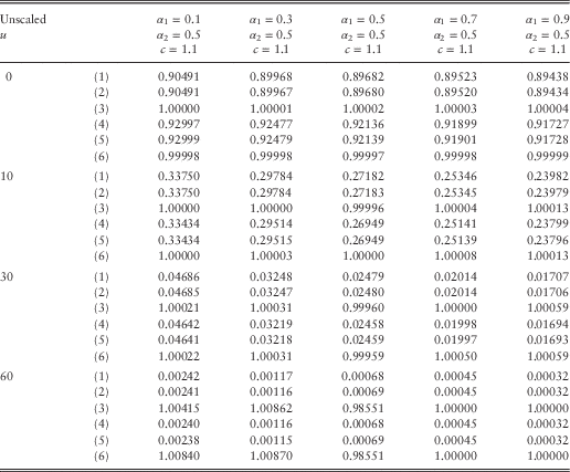
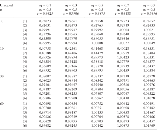
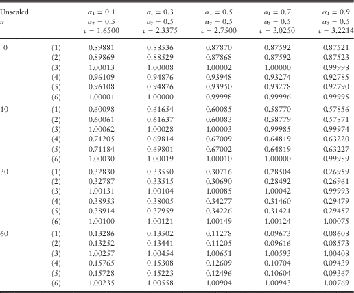
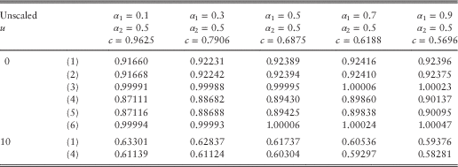
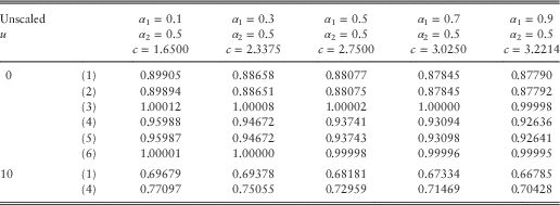
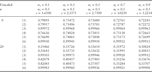
Tables 1–3 show exact and approximate values for the ultimate ruin probability in the continuous time model when the individual claim amounts are exponentially distributed. To find ψ i (u) we have applied the methods of Li & Lu (Reference Li and Lu2008). The key for these tables is as follows:
-
(1) denotes the approximation to ψ 1(u),
-
(2) denotes the exact value of ψ 1(u),
-
(3) denotes the ratio of the value in (1) to that in (2),
-
(4) denotes the approximation to ψ 2(u),
-
(5) denotes the exact value of ψ 2(u),
-
(6) denotes the ratio of the value in (4) to that in (5).
We note the following points about Tables 1–3.
-
(i) In Tables 1 and 3 most of the approximations agree with the exact values up to four decimal places with the best results being obtained in Table 1 when α 1=α 2=0.5. The approximations in Table 2 are in agreement with the exact values up to three decimal places. In this table we get better approximations when α 1<0.9.
-
(ii) The ratios of the approximate values to the exact values do not show consistent patterns. For example, in Table 2 when α 1=0.7, 0.9, the ratios are greater than 1, whereas for α 1=0.1, 0.3, 0.5, the ratios are mostly less than 1. In Table 3, unlike in Table 2, when α 1=0.1, 0.3, 0.5, the ruin probability is overstated and when α 1=0.7, 0.9, and u=0, 10, all the approximations understate the exact values. We cannot observe any pattern for the ratios with different values of u and α 1 in Table 1.
-
(iii) Generally, we observe that the approximation in the case of exponential claims performs better for small values of u and α 1.
-
(iv) Regarding the relationship between ψ 1(u) and ψ 2(u) we can see that as u increases, ψ 1(u) gets closer to ψ 2(u). In Table 2, where E[S 1]>E[S 2], values of ψ 1(u) are always greater than ψ 2(u). In Table 3, where E[S 1]<E[S 2], ψ 1(u) is always less than ψ 2(u), but in Table 1, where E[S 1]=E[S 2], we cannot identify any consistent pattern between ψ 1(u) and ψ 2(u) except that for a given value of u if ψ 1(u)>ψ 2(u), this relationship will hold across the table regardless of the mean of the sojourn time. In fact, we can see that the values of ψ 1(u) and ψ 2(u) are very close.
Exponential claims, with E[S 1]=E[S 2].

Exponential claims, with E[S 1]>E[S 2].

Exponential claims, with E[S 1]<E[S 2].

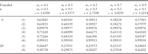
Tables 4–6 show the approximate values of ψ i (u) in the continuous time model for claim sizes with Pareto distributions, and the key to these tables is the same as in Tables 1–3.
Pareto claims when E[S 1]=E[S 2].

Pareto claims when E[S 1]>E[S 2].

Pareto claims when E[S 1]<E[S 2].

Unlike in the classical risk model, the expression for the ruin probability when u=0 is dependent on the individual claim amount distributions, as ψ ij (0) depends on the Laplace transform of the claim amount distributions in the continuous time case (and on their probability generating functions in the discrete time case). However, we can see that ruin probabilities when u=0 for exponential and Pareto claims are fairly close for Cases 1 and 4, Cases 2 and 5, and Cases 3 and 6. We can identify a similar pattern between the approximate values of the ruin probability with claim amounts following Pareto distributions and claim amounts following exponential distributions. For example, in Table 5 when α 1=0.7, 0.9, the ruin probability when u=0 is overstated, whereas for α 1=0.1, 0.3, it is understated, which is different to Table 6 in which the ruin probability is overstated for α 1=0.1, 0.3, and understated for α 1=0.7, 0.9. In addition, similar to Table 1 no particular pattern can be observed for Table 5.
We conclude from these tables that our algorithm provides good approximations to the exact values in the continuous time Markov-modulated model.
4.2. Approximations to H 1(u, y) and H 2(u, y)
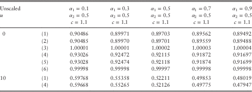
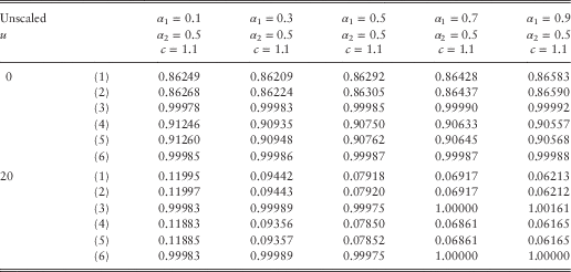
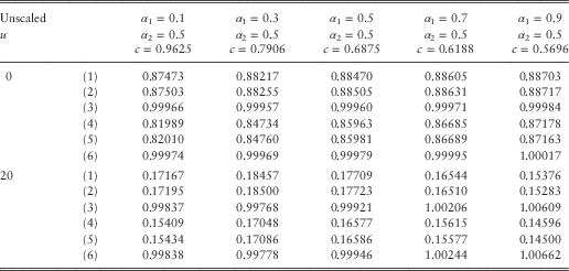
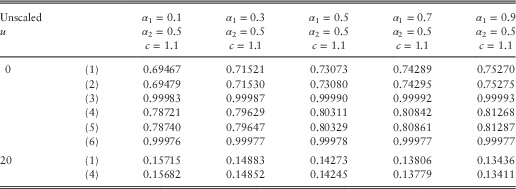
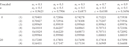
Tables 7–9 (exponential claims) and Tables 10–12 (Pareto claims) show approximations to the probability and severity of ruin for initial surplus levels u=0 and u=20. We performed calculations for different values of y, but only show the results for y=3. In the case of exponential claims, we can calculate exact values of the probability and severity of ruin in the continuous time model when u≥0 by applying the memoryless property of the exponential distribution to write
 $$H_{{ij}} \left( {u,y} \right)\,{\equals}\,\psi _{{ij}} (u)\left( {1{\minus}e^{{{\minus}\gamma _{j} \,y}} } \right)$$
for i, j=1, 2. The key for these tables is as follows:
-
(1) denotes the approximation to H 1(u, y),
-
(2) denotes the exact value of H 1(u, y),
-
(3) denotes the ratio of the value in (1) to that in (2),
-
(4) denotes the approximation to H 2(u, y),
-
(5) denotes the exact value of H 2(u, y),
-
(6) denotes the ratio of the value in (4) to that in (5).
Exponential claims, y=3 and E[S 1]=E[S 2].

Exponential claims, y=3 and E[S 1]>E[S 2].

Exponential claims, y=3 and E[S 1]<E[S 2].

Pareto claims, y=3 and E[S 1]=E[S 2].

Pareto claims, y=3 and E[S 1]>E[S 2].

Pareto claims, y=3 and E[S 1]<E[S 2].

We note the following points about Tables 7–9.
-
(i) In Table 8 the approximations for α 1=0.1, 0.3, 0.5 understate the exact values, and for α 1=0.7, 0.9 overstate the exact values when u>0. This is in line with what we had observed for the ruin probability.
-
(ii) In Table 9 all approximations for α 1=0.5, 0.7, 0.9 understate the exact values and in this case the approximation performs better than in other cases.
-
(iii) Regarding the relationship between H 1(u, y) and H 2(u, y), we can see that similar to the probability of ruin, as u increases the values for H 1(u, y) and H 2(u, y) become closer to each other. In Tables 7 and 8 we observe that H 1(u, y)<H 2(u, y) for a given value of u, but there is no such relationship between H 1(u, y) and H 2(u, y) in Table 9.
Tables 10–12 show approximations to the probability and severity of ruin when claim amounts follow Pareto distributions. The exact values in the case u=0 have been calculated using techniques described in Li & Lu (Reference Li and Lu2008). We note that all approximations for u=0 are less than the exact values. In Table 10 we note that H 1(0, y)<H 2(0, y), while H 1(20, y)>H 2(20, y). However, in Table 11, where E[S 1]>E[S 2], H 1(u, y)>H 2(u, y), while in Table 12, where E[S 1]<E[S 2], H 1(u, y)<H 2(u, y).
Overall, our algorithm performs well and provides good approximations. Calculations for other values of y showed a similar trend to that observed in Dickson & Waters (Reference Dickson and Waters1992) for the classical risk model, namely that in the case of exponential claims, the quality of the approximations improved as y increased.
5. The Probability of Ruin in Finite Time
In this section, we consider the probability of ruin in finite time. First, we provide recursive formulae which can be used to approximate ψ i (u, t) for i∈M. Then, we explain how we can adapt the truncation method of De Vylder & Goovaerts (Reference De Vylder and Goovaerts1988) to improve the computational efficiency of our numerical algorithm.
Theorem 5.1 For u=0, 1, 2, …
 $$\psi _{i}^{d} \left( {u,1} \right)\,{\equals}\,\mathop{\sum}\limits_{j\,{\equals}\,1}^m \mathop{\sum}\limits_{x\,{\equals}\,u{\plus}1}^\infty g_{{ij}} (x)\,{\equals}\,1{\minus}G_{i} (u)$$
and for t>1
 $$\psi _{i}^{d} \left( {u,t} \right)\,{\equals}\,\psi _{i}^{d} \left( {u,1} \right){\plus}\mathop{\sum}\limits_{j\,{\equals}\,1}^m \mathop{\sum}\limits_{x\,{\equals}\,0}^u g_{{ij}} (x)\psi _{j}^{d} \left( {u{\plus}1{\minus}x,t{\minus}1} \right)$$
Proof: We first consider
 $$\psi _{i}^{d} (u,1)$$
. For ruin to occur in the first time period, we require that the aggregate claim amount in the first time period exceeds u. Hence (5.1) follows. For t>1 we note that if ruin occurs at or before time t, then either
-
(i) Y 1>u so that ruin occurs at time 1, or
-
(ii) Y 1=x, for x=0, 1, 2, … , u, and ruin occurs in the next t−1 time periods, from surplus level u+1−x at time 1.
Thus (5.2) follows.
We can use formulae (5.1) and (5.2) to calculate finite time ruin probabilities recursively. First, we need to calculate
 $$\psi _{i}^{d} (w,1)$$
for w=0, 1, 2, … , u+t−1 from (5.1) for i=1, 2, … , m, then using equation (5.2) we calculate
 $$\psi _{i}^{d} (w,2)$$
for w=0, 1, 2, … , u+t−2 and i=1, 2, … , m. We continue this process until we calculate
 $$\psi _{i}^{d} (w,t)$$
for w=0, 1, 2, … , u for i=1, 2, … , m. This method requires much computation time, particularly when the values of u and t are large. Since many of the probabilities used in the calculations will be very small, we can reduce the number of calculations involved by adapting the truncation method of De Vylder & Goovaerts (Reference De Vylder and Goovaerts1988) which is based on ignoring small probabilities. Let k
i,1 be the least integer such that G
i
(k
i,1)≥1−
 $$\epsilon$$
, where
 $$\epsilon$$
is a small positive value. Then let
 $$g_{{ij}}^{{\epsilon}} (x)\,{\equals}\,\left\{ {\matrix{ {g_{{ij}} (x)} \hfill & {{\rm for}\,\,x\,{\equals}\,0,1,2,\ldots{\!},k_{{i,1}} } \hfill \cr 0 \hfill & {{\rm for}\,\,x\,{\equals}\,k_{{i,1}} {\plus}1,k_{{i,1}} {\plus}2,\,\ldots\,} \hfill \cr } } \right.$$
and
 $$\psi _{i}^{{d{\epsilon}}} \left( {u,1} \right)\,{\equals}\,\left\{ {\matrix{ {1{\minus}G_{i} (u)} \hfill & {{\rm for}\,\,u\,{\equals}\,0,1,2,\ldots{\!},k_{{i,1}} } \hfill \cr 0 \hfill & {{\rm for}\,\,u\,{\equals}\,k_{{i,1}} {\plus}1,k_{{i,1}} {\plus}2,\,\ldots\,} \hfill \cr } } \right.$$
Further, let k
i,t
be the least integer such that
 $$\psi _{i}^{d} (k_{{i,t}} ,t{\minus}1)\geq {\epsilon}$$
. Then we will calculate
 $$\psi _{j}^{d} (u,t)$$
for u=0, 1, 2, … , k
j,t
, and otherwise set it equal 0. Thus, we can evaluate the finite time ruin probability from
 $$\psi _{i}^{{d{\epsilon}}} \left( {u,t} \right)\,{\equals}\,\psi _{i}^{{d{\epsilon}}} \left( {u,1} \right){\plus}\mathop{\sum}\limits_{j\,{\equals}\,1}^m \mathop{\sum}\limits_{x\,{\equals}\,L}^U g_{{ij}}^{{\epsilon}} (x)\psi _{j}^{{d{\epsilon}}} \left( {u{\plus}1{\minus}x,t{\minus}1} \right)$$
where L=max(0, u+1−k
j,t−1) and U=min(u, k
i,1). We can demonstrate that similar to the classical risk model, the error introduced by using (5.3) and (5.4) in place of (5.1) and (5.2) can be bounded. We have
 $\psi _{i}^{d} \left( {u,1} \right){\minus}{\epsilon}\leq \psi _{i}^{{d{\epsilon}}} \left( {u,1} \right)\leq \psi _{i}^{d} \left( {u,1} \right)$
and for t=2, 3, …
 $$\psi _{i}^{d} \left( {u,t} \right){\minus}2t{\epsilon}\leq \psi _{i}^{{d{\epsilon}}} \left( {u,t} \right)\leq \psi _{i}^{d} \left( {u,t} \right)$$
As the proof contains no new ideas, we omit it. See De Vylder & Goovaerts (Reference De Vylder and Goovaerts1988) or Dickson & Waters (Reference Dickson, Egídio dos Reis and Waters1991) for details.
5.1. The density of the time to ruin
Define
 $$w_{i} \left( {u,t} \right)\,{\equals}\,{\partial \over {\partial t}}\psi _{i} \left( {u,t} \right)$$
to be the (defective) density of the time of ruin in the continuous time Markov-modulated model (given initial state i). Adjusting the approach of Dickson & Waters (Reference Dickson and Waters2002), we can approximate w i (u, t) at time t=j/cβ by
 $$c \beta \left[ {\psi _{i} \left( {u,{j \over {c\beta }}} \right){\minus}\psi _{i} \left( {u,{{j{\minus}1} \over {c\beta }}} \right)} \right]$$
for j=1, 2, … , and we can approximate ψ i (u, j/(cβ)) using formulae (5.3) and (5.4). Dividing this by our approximation to ψ i (u) from the algorithm described in section 4 gives us an approximation to the proper density of the time of ruin.
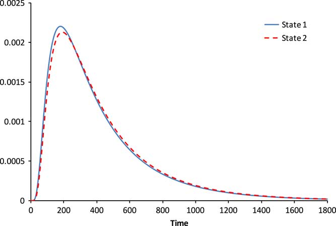
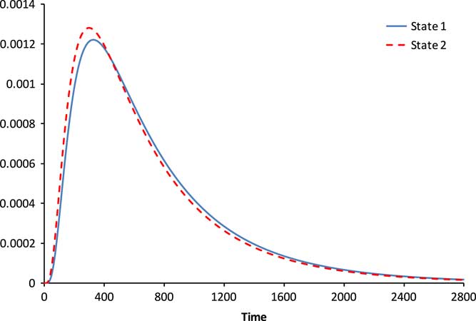
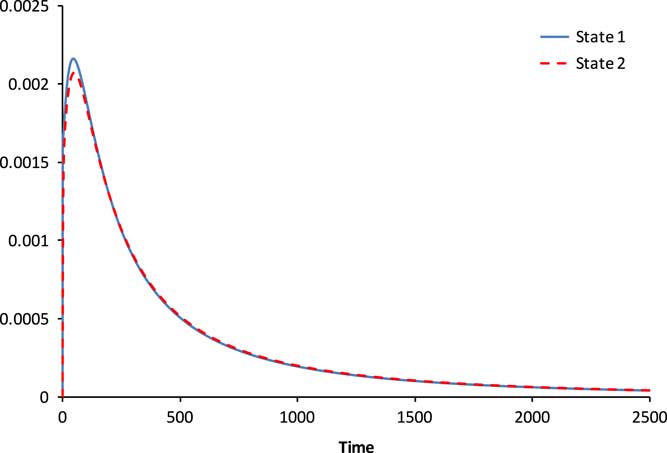
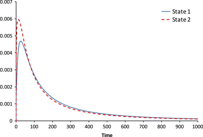
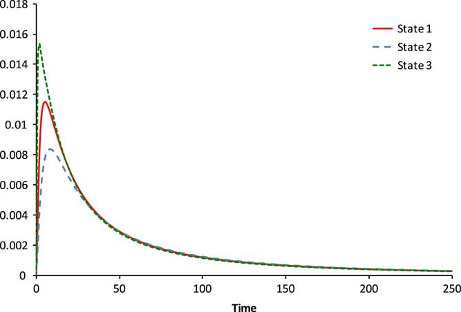
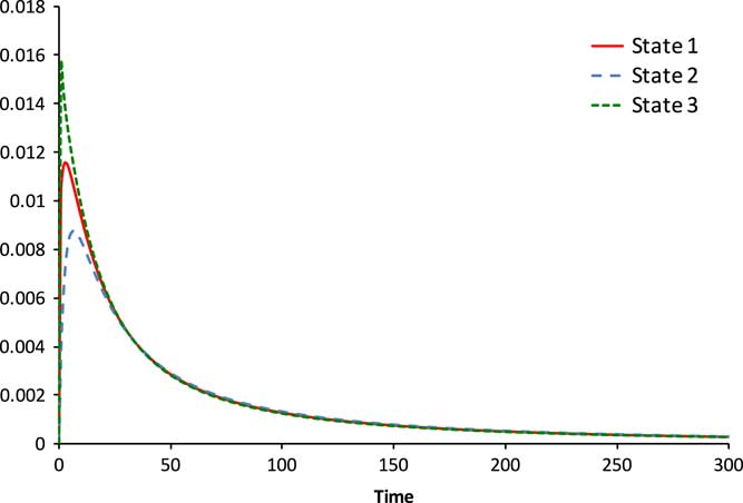
We now illustrate the density of the time of ruin for four of six cases that we discussed in section 4. In all figures α 1=0.1, α 2=0.5, β=20, and the implied loading factor is 0.1. We remark that the accuracy of the approximations for the scaling factor 20 is only up to two decimal places. However, this precision is sufficient for our purpose here, which is to illustrate the shape of the density functions.
Figures 1 and 2 show our approximations to the proper density of the time of ruin for exponential claim amounts. For these figures, we have chosen the initial surplus such that the ultimate ruin probability is in the range of practical interest. Figure 1 shows the situation when E[S 1]>E[S 2], ψ 1(40)=0.03418 and ψ 2(40)=0.03071. In Figure 2 we have ψ 1(120)=0.02304 and ψ 2(120)=0.02721. This figure presents the density of the time of ruin, given that ruin occurs when E[S 1]<E[S 2]. Figures 3 and 4 illustrate the density of the time of ruin, given that ruin occurs when claim amounts follow Pareto distributions and the initial surplus is 40. The pattern of these graphs is the same as the graphs for the exponential claim amounts. We can observe that the common feature of all these figures is that they are all positively skewed and the skewness is heightened when claim amounts follow Pareto distributions. These figures are consistent with plots of the density of the time of ruin in the classical risk model; see, for example, Dickson & Waters (Reference Dickson and Waters2002).
Case 2: ψ 1(40)=0.03418 and ψ 2(40)=0.03071.

Case 3: ψ 1(120)=0.02304 and ψ 2(120)=0.02721.

Case 5: ψ 1(40)=0.34427 and ψ 2(40)=0.33677.

Case 6: ψ 1(40)=0.43292 and ψ 2(40)=0.47021.

Although we have not shown them here, the graphs of the density of the time of ruin when E[S 1]=E[S 2] virtually coincide, which is perhaps not surprising given that in this case the ultimate ruin probabilities in states 1 and 2 are very close.
5.2. The density of the ruin time for
$${\mib m \,\gt}\, {\bf 2}$$

We now apply our numerical procedure to the case m>2. There is nothing new in the application of our algorithms except the calculation of the transition probabilities for which we suggest the following two methods, and our experiments show both give very similar results:
-
(i)
$$p_{{ii}} \,{\equals}\,e^{{{\minus}\alpha _{i} /c\beta }} $$
and
$$p_{{ij}} \,{\equals}\,\left( {1{\minus}e^{{{\minus}\alpha _{i} /c\beta }} } \right)\alpha _{{ij}} /\alpha _{i} $$
for i≠j, -
(ii) p ii =1−α i /cβ and p ij =α ij /cβ for i≠j.


We remark that method (i) is in fact the method that we have used in our numerical calculations for the case m=2, and the calculations for this section are based on this approach.
We consider a three-state model with the following intensity matrix:
 $$\left( {\matrix{ {{\minus}0.6} & \;\;\;{0.2} & \;\;\;{0.4} \cr \;\;\; {0.1} & {{\minus}0.3} & \;\;\;{0.2} \cr \;\;\;{0.5} & \;\;\;{0.3} & {{\minus}0.8} \cr } } \right)$$
We calculate c=1.1355 in the continuous time model so that relationship (2.2) is satisfied and set β=20. Figure 5 shows our approximation to the (defective) density of the time of ruin when λ i =1 for i=1, 2, 3 and individual claim amounts are exponentially distributed with means 1, 0.5 and 2. Figure 6 illustrates the situation when individual claim amounts follow Pareto distributions with parameters a 1=2, b 1=1, a 2=3, b 2=1 and a 3=2, b 3=1 and λ 1=λ 2=1 and λ 3=2. We observe that the common features of Figures 5 and 6 are that they are positively skewed and the graph for the (defective) density of the time of ruin in state 3, where E[S 3] is higher than the expected aggregate claim amount in the two other states, is located on the top and for state 2, where E[S 2] is less than that in states 1 and 3, is at the bottom with the graph for state 1, where E[S 3]>E[S 1]>E[S 2], being in the middle.
Exponential claims.

Pareto claims.

If we let the finite time period be sufficiently large, the cumulative distribution function of the time of ruin can give us an approximation to the ultimate ruin probability for an m-state model; at the very least it provides a lower bound. We observed different features in the case of exponential and Pareto claims, with the distribution function of the time of ruin appearing to converge for smaller values of t in the case of exponential claims. For example, our observation from graphs of the cumulative distribution function of the time of ruin for individual claim amounts with the above exponential distributions suggests that ψ i (10) for i=1, 2 and 3 is close to 0.559, 0.524 and 0.581, respectively, and when individual claim amounts follow the above Pareto distributions we can say that good lower bounds for ψ i (10) for i=1, 2 and 3 are 0.608, 0.583 and 0.622, respectively. This method can be extended easily to m>3. However, we cannot verify the accuracy of the resulting ψ i (u) values.
We remark that Li et al. (Reference Li, Dickson and Li2014) considered the density of the time of ruin in the continuous time Markov-modulated model. They derived a general expression for w i (u, t) and, using numerical integration, implemented their formulae for u=0, 5 when claim amounts in state 1 follow an exponential distribution and in state 2 follow an Erlang(2) distribution. As with the classical risk model, the formula for the (defective) density of the time of ruin in the Markov-modulated risk model, is expressed in terms of the density of the aggregate claim amount. However, in contrast to the classical risk model, the solution to the integro-differential equation that is satisfied by the distribution of the aggregate claim amount does not lead to a neat expression. This issue arises as we must calculate the aggregate claims distributions in matrix form under the Markov-modulated risk model. In general, it appears that our approach for the approximation of w i (u, t) is more straightforward than their numerical integration.
Acknowledgements
None.
Appendix
In the proofs of Theorems 3.1 and 3.2 we assumed that
 $$\mathop{\sum}\nolimits_{u\,{\equals}\,0}^\infty \psi _{i}^{d} (u)\,\lt\,\infty.$$
We now state conditions under which this is true.
Let
d
L
i
be a discrete random variable representing the maximum aggregate loss, given initial state i, i=1, 2. Then the distribution function of
d
L
i
is
 $$\delta _{i}^{d} (u)$$
, and the first moment is given by
 $$E\left[ {^{d} L_{i} } \right]\,{\equals}\mathop{\sum}\limits_{u\,{\equals}\,0}^\infty \psi _{i}^{d} (u)\,{\equals}\,\mathop{\sum}\limits_{u\,{\equals}\,0}^\infty {\rm Pr}\left( {^{d} L_{i} \,\gt\,u} \right)$$
Therefore, we can conclude that
 $$\mathop{\sum}\nolimits_{u\,{\equals}\,0}^\infty \psi _{i}^{d} (u)\,\lt\,\infty$$
, if E[
d
L
i
] exists. The next result gives an expression for E[
d
L
i
] and is motivated by the ideas of Dufresne (Reference Dufresne1988).
Theorem For i=1, 2, the first moment of the maximum aggregate loss is given by
 $$E\left[ {^{d} L_{i} } \right]\,{\equals}\,{\minus}J_{i}^{'} (1)$$
where
 $$J_{1} \left( s \right)\,{\equals}\,{{1{\plus}\left( {1{\minus}s^{{{\minus}1}} } \right)\left( {\psi _{1}^{d} \left( 0 \right)} \right.\tilde{g}_{{11}} \left( s \right){\plus}\psi _{2}^{d} \left( 0 \right)\tilde{g}_{{12}} \left. {\left( s \right)} \right){\minus}\tilde{g}_{1} \left( s \right){\plus}s^{{{\minus}1}} \tilde{g}_{{12}} \left( s \right)J_{2} \left( s \right)} \over {1{\minus}s^{{{\minus}1}} \tilde{g}_{{11}} \left( s \right)}}$$
and
 $$J_{2} \left( s \right)\,{\equals}\,{{1{\plus}\left( {1{\minus}s^{{{\minus}1}} } \right)\left( {\psi _{1}^{d} \left( 0 \right)} \right.\tilde{g}_{{21}} \left( s \right){\plus}\psi _{2}^{d} \left( 0 \right)\tilde{g}_{{22}} \left. {\left( s \right)} \right){\minus}\tilde{g}_{2} \left( s \right){\plus}s^{{{\minus}1}} \tilde{g}_{{21}} \left( s \right)J_{1} \left( s \right)} \over {1{\minus}s^{{{\minus}1}} \tilde{g}_{{22}} \left( s \right)}}$$
Proof: We begin with
 $$\psi _{i}^{d} (u)\,{\equals}\,\mathop{\sum}\limits_{j{\equals}1}^2 g_{{ij}} (0)\psi _{j}^{d} \left( {u{\plus}1} \right){\plus}\mathop{\sum}\limits_{j\,{\equals}\,1}^2 \mathop{\sum}\limits_{x\,{\equals}\,1}^u g_{{ij}} (x)\psi _{j}^{d} \left( {u{\plus}1{\minus}x} \right){\plus}\mathop{\sum}\limits_{j\,{\equals}\,1}^2 \mathop{\sum}\limits_{x\,{\equals}\,u{\plus}1}^\infty g_{{ij}} (x)$$
and define
 $$\eqalignno{ d_{i} (0)\,& {\equals}\, \psi _{i}^{d} (0) \cr &{\equals} \mathop{\sum}\limits_{j\,{\equals}\,1}^2 g_{{ij}} (0)\psi _{j}^{d} (1){\plus}\mathop{\sum}\limits_{j\,{\equals}\,1}^2 \mathop{\sum}\limits_{x\,{\equals}\,1}^u g_{{ij}} (x)\psi _{j}^{d} \left( {1{\minus}x} \right){\plus}\mathop{\sum}\limits_{j\,{\equals}\,1}^2 \mathop{\sum}\limits_{x\,{\equals}\,u{\plus}1}^\infty g_{{ij}} (x) $$
and
 $$\eqalignno{ d_{i} (u)\,{\equals}\, & \psi _{i}^{d} (u){\minus}\psi _{i}^{d} \left( {u{\minus}1} \right) \cr {\equals} & \mathop{\sum}\limits_{j\,{\equals}\,1}^2 g_{{ij}} (0)\psi _{j}^{d} \left( {u{\plus}1} \right){\plus}\mathop{\sum}\limits_{j\,{\equals}\,1}^2 \mathop{\sum}\limits_{x\,{\equals}\,1}^u g_{{ij}} (x)\psi _{j}^{d} \left( {u{\plus}1{\minus}x} \right){\plus}1{\minus}G_{i} (u) \cr & {\minus}\mathop{\sum}\limits_{j\,{\equals}\,1}^2 g_{{ij}} (0)\psi _{j}^{d} (u){\minus}\mathop{\sum}\limits_{j\,{\equals}\,1}^2 \mathop{\sum}\limits_{x\,{\equals}\,1}^{u{\minus}1} g_{{ij}} (x)\psi _{j}^{d} \left( {u{\minus}x} \right){\minus}1{\plus}G_{i} \left( {u{\minus}1} \right) $$
Then, by noting that
 $$\psi _{i}^{d} (1)\,{\equals}\,d_{i} (1){\plus}d_{i} (0)$$
, equation (A.4) can be written as
 $$d_{i} (u)\,{\equals}\,\mathop{\sum}\limits_{j\,{\equals}\,1}^2 g_{{ij}} (0)d_{j} \left( {u{\plus}1} \right){\plus}\mathop{\sum}\limits_{j\,{\equals}\,1}^2 g_{{ij}} (u)d_{j} (0){\plus}\mathop{\sum}\limits_{j\,{\equals}\,1}^2 \mathop{\sum}\limits_{x\,{\equals}\,1}^u g_{{ij}} (x)d_{j} \left( {u{\plus}1{\minus}x} \right){\minus}g_{i} (u)$$
Further, we define
 $$J_{i} (s)\,{\equals}\,d_{i} (0){\plus}\mathop{\sum}\limits_{n\,{\equals}\,1}^\infty s^{n} d_{i} (n)$$
. Then, by (A.3) and with the usual convention that
 $$\mathop{\sum}\nolimits_{j\,{\equals}\,a}^b {\equals}\,0$$
when b<a, we have
 $$\eqalignno{ J_{i} (s)\,{\equals} & \mathop{\sum}\limits_{j\,{\equals}\,1}^2 {g_{{ij}} (0)\left( {d_{j} (1){\plus}d_{j} (0)} \right){\plus}1{\minus}g_{i} (0){\plus}\mathop{\sum}\limits_{j\,{\equals}\,1}^2 \mathop{\sum}\limits_{n\,{\equals}\,1}^\infty s^{n} \left( {g_{{ij}} (0)d_{j} (n{\plus}1} \right)} \cr & {\plus}g_{{ij}} (n)d_{j} (0){\minus}g_{i} (n){\plus}\mathop{\sum}\limits_{x\,{\equals}\,1}^n g_{{ij}} (x)d_{j} \left( {n{\plus}1{\minus}x)} \right) \cr {\equals} &\mathop{\sum}\limits_{j\,{\equals}\,1}^2 g_{{ij}} (0)\left( {d_{j} (1){\plus}d_{j} (0)} \right){\plus}1{\minus}g_{i} (0){\plus}\mathop{\sum}\limits_{j\,{\equals}\,1}^2 \left( {\tilde{g}_{{ij}} (s){\minus}g_{{ij}} (0)} \right)d_{j} (0) \cr & {\plus}s^{{{\minus}1}} \mathop{\sum}\limits_{j\,{\equals}\,1}^2 g_{{ij}} (0)\left( {J_{j} (s){\minus}sd_{j} \left( 1 \right){\minus}d_{j} (0)){\minus}(\tilde{g}_{i} (s){\minus}g_{i} (0)} \right) \cr & {\plus}s^{{{\minus}1}} \mathop{\sum}\limits_{j\,{\equals}\,1}^2 \left( {\tilde{g}_{{ij}} (s){\minus}g_{{ij}} (0))(J_{j} (s){\minus}d_{j} (0)} \right) $$
Rearranging (A.6), formulae (A.1) and (A.2) follow.
Applying formulae (A.1) and (A.2), we find
 $$\eqalignno{ E\left[ {^{d} L_{1} } \right]\,{\equals}\, & {{{\minus}1} \over {2p_{{21}} p_{{12}}^{2} (\mu _{2} {\minus}1){\plus}2p_{{12}} p_{{21}}^{2} (\mu _{1} {\minus}1)}}\left\{ {2\psi _{1}^{d} (0)[p_{{21}}^{2} \left( {p_{{11}} {\minus}\mu _{{11}} } \right)} \right. \cr & {\plus}p_{{12}}^{2} p_{{21}} \left( {1{\minus}\mu _{2} } \right){\plus}p_{{11}} p_{{21}}^{2} \left( {\mu _{1} {\minus}1} \right)]{\plus}2\psi _{2}^{d} (0)[p_{{12}} p_{{21}}^{2} \left( {1{\minus}\mu _{1} } \right) \cr & {\plus}p_{{12}}^{2} \left( {p_{{22}} {\minus}\mu _{{22}} } \right){\plus}p_{{12}} p_{{21}}^{2} \left( {\mu _{1} {\minus}1} \right)]{\plus}\mu _{1} p_{{21}}^{2} \left( {1{\plus}p_{{11}} {\minus}2\mu _{{11}} } \right) \cr & \left. {{\plus}\mu _{2} p_{{12}}^{2} \left( {1{\plus}p_{{22}} {\minus}2\mu _{{22}} } \right){\minus}p_{{12}} p_{{21}} \left( {\left( {\mu _{2} } \right)_{1} \:p_{{21}} {\plus}\left( {\mu _{2} } \right)_{2} \:p_{{12}} } \right){\minus}2\mu _{1} p_{{21}}^{2} \left( {\mu _{1} {\minus}1} \right)} \right\} $$
where
 $$(\mu _{2} )_{i} {\equals}\mathop{\sum}\limits_{j{\equals}1}^2 \mathop{\sum}\limits_{x{\equals}1}^\infty x^{2} \:g_{{ij}} (x)$$
for i=1, 2, and
 $$\eqalignno { E\left[ {^{d} L_{2} } \right]{\equals} & {{{\minus}1} \over {2p_{{21}} p_{{12}}^{2} \left( {\mu _{2} {\minus}1} \right){\plus}2p_{{12}} p_{{21}}^{2} \left( {\mu _{1} {\minus}1} \right)}}\left\{ {2\psi _{1}^{d} (0)[p_{{21}}^{2} \left( {p_{{11}} {\minus}\mu _{{11}} } \right)} \right. \cr & {\plus}p_{{12}}^{2} p_{{21}} \left( {1{\minus}\mu _{2} } \right){\minus}p_{{11}} p_{{21}} p_{{12}} \left( {\mu _{2} {\minus}1} \right)]{\plus}2\psi _{2}^{d} (0)[p_{{12}} p_{{21}}^{2} \left( {1{\minus}\mu _{1} } \right) \cr & {\plus}p_{{12}}^{2} \left( {p_{{22}} {\minus}\mu _{{22}} } \right){\minus}p_{{21}} p_{{12}}^{2} \left( {\mu _{2} {\minus}1} \right)]{\minus}\mu _{1} p_{{21}}^{2} \left( {1 \cr & {\plus}p_{{11}} {\minus}2\mu _{{11}} } \right) \cr & \left. { {\minus}\mu _{2} p_{{12}}^{2} \left( {1{\plus}p_{{22}} {\minus}2\mu _{{22}} } \right){\plus}p_{{12}} p_{{21}} ((\mu _{2} )_{1} \:p_{{21}} {\plus}(\mu _{2} )_{2} \:p_{{12}} ){\plus}2\mu _{1} p_{{21}} p_{{12}} \left( {\mu _{2} {\minus}1} \right)} \right\} $$
From (A.7) and (A.8) we can conclude that E[ d L 1] and E[ d L 2] exist on the condition that the moments, that is (μ 2) i exist for i=1, 2. From remark 2 in Chen et al. (Reference Chen, Yuen and Guo2014) we note that the denominators in each of (A.7) and (A.8) are negative.