



1. Introduction
The interaction between a detonation wave and a wedge is important considering its application in propulsion systems (Wolański Reference Wolański2013). Detonation reflections over complex geometries – such as double wedges – are important for the design of pulse detonation engines and rotating detonation engines. Regular reflection (RR) or Mach reflection (MR) occurs when a planar detonation wave collides with a wedge (Ong Reference Ong1955; Akbar Reference Akbar1971). The RR configuration consists of the incident wave
 $i$
and the reflected wave r, which can be observed when the wedge angle (
 $\varphi$
) exceeds the MR-RR transition angle (
 $\varphi _c$
). The MR process can be analysed in the following way. When the incident detonation wave passes over the compressive corner, the gas flow induced by the moving detonation is disturbed. As a result, a family of cylindrical compression waves is generated at the leading edge of the wedge. These compression waves propagate with the local sound speed relative to the local flow velocity, and coalesce forming a shock–shock (or a detonation–detonation as named by Li & Ben-Dor Reference Li and Ben-Dor1998) that intersects with the incident detonation. Consequently, a triple point T forms, associated with an incident detonation
 $i$
, a reflected shock r, a straight Mach stem m, and a slipstream s. When a plane detonation wave encounters a double wedge (figure 1
a), different types of reflection processes can be observed, depending on the wedge angles. Ben-Dor, Dewey & Takayama (Reference Ben-Dor, Dewey and Takayama1987), Ben-Dor et al. (Reference Ben-Dor, Dewey, McMillin and Takayama1988) and Takayama & Ben-Dor (Reference Takayama and Ben-Dor1988) have studied the reflection of a planar shock wave over a double wedge both analytically and experimentally. In their analytical study, seven inert shock wave reflection processes (figure 1
b) could be determined. For the scenario concerned in this study (the grey region in figure 1
b), three MRs occur successively. Figure 2 shows a hypothetical MR process of a detonation wave over a concave double wedge. Over the first surface, a classical MR phenomenon is indisputable (MR1). As the Mach stem m
 $_1$
encounters the second wedge, a secondary MR configuration (m
 $_1$
serves as the incident wave) is expected (MR2). After the interaction of the two triple points (T
 $_1$
and T
 $_2$
), a tertiary MR associated with the original detonation wave
 $i$
can be formed (MR3). There are currently no reported studies on the specific characteristics of these three MRs of detonations over a concave double wedge. Only a numerical study conducted by Li et al. (Reference Li, Pan, Jiang, Shi, Zhu and Quaye2022) reported seven reflection processes of detonation reflections over concave and convex double wedges. However, the specific characteristics of reflection processes were not investigated in their study.
Sketch of a double-wedge reflector and regions of reflection processes over a double-wedge surface. Here,
 $S_1$
is the length of the first surface,
 $S_2$
is the length of the second surface,
 $\varphi _1$
is the angle of the first wedge,
 $\varphi _2$
is the angle of the second wedge, and
 $\Delta \varphi=\varphi_2-\varphi_1$
.

The primary MR over the first surface (MR1) is a classical pseudo-steady MR. Up to now, numerous investigations have been devoted to exploring the MR characteristics of gaseous detonations over a plane wedge (Edwards, Walker & Nettleton Reference Edwards, Walker and Nettleton1984; Meltzer et al. Reference Meltzer, Shepherd, Akbar and Sabet1993; Li, Ben-Dor & Gronig Reference Li, Ben-Dor and Gronig1997; Shepherd, Schultz & Akbar Reference Shepherd, Schultz and Akbar1999; Thomas & Williams Reference Thomas and Williams2002; Fortin, Liu & Lee Reference Fortin, Liu and Lee2015; Li et al. Reference Li, Ren, Wang and Ning2018; Chen, Ma & Wang Reference Chen, Ma and Wang2023; Zhou, Ma & Wang Reference Zhou, Ma and Wang2024). Due to the intrinsic thickness of the wave front, the detonation MR process exhibits localised self-similarity. Near the leading edge of the wedge, the triple-point trajectory is consistent with that of an inert shock (frozen limit). In the far field, the self-similarity can be recovered asymptotically, which is called the ‘equilibrium limit’. Li, Ning & Lee (Reference Li, Ning and Lee2015) and Li & Lee (Reference Li and Lee2016) confirmed the localised self-similarity of MR of Zeldovich-von Neumann-Döring (ZND) detonations and cellular detonations by numerical simulations. Fortin et al. (Reference Fortin, Liu and Lee2015) and Li et al. (Reference Li, Ren, Wang and Ning2018) experimentally confirmed the local self-similar triple-point trajectories of detonation MRs in various mixtures. Zhou et al. (Reference Zhou, Ma and Wang2024) indicated the significant influence of velocity deficits on the self-similarity of MR. As illustrated in figure 2, the triple-point trajectory angle decreases from
 $\theta$
(near field) to
 $\chi$
(far field). Assuming that the Mach stem is straight, the two angles can be calculated using the non-reactive theories (Whitham Reference Whitham1957; von Neumann Reference von Neumann1963) and the modified theories (Li et al. Reference Li, Ben-Dor and Gronig1997; Li & Ben-Dor Reference Li and Ben-Dor1998), respectively. However, Li et al. (Reference Li, Ren, Wang and Ning2018) indicated that with a large wedge angle (more than
 $30^\circ$
), the final asymptotic triple-point trajectory angle is not in agreement with the theoretical results.
Sketch of the MR process over a concave double wedge. The MR structures evolve at different time instants. As the incident detonation wave propagates, three MR structures appear in sequence. Here,
 $i$
is the incident wave, r is the reflection wave, m is the Mach stem, T is the triple point of the MR,
 $\varphi$
is the wedge angle,
 $\theta$
is the triple-point trajectory angle in the frozen limit,
 $\chi$
is the triple-point trajectory angle in the equilibrium limit, Q is the collision point of two triple points, and
 $\delta$
is the deflection angle of the detonation surface.

The secondary MR over the second surface (MR2) is an MR of an overdriven detonation wave. The Mach stem m
 $_1$
, which is essentially an overdriven detonation wave, serves as the incident wave in MR2 (see figure 2). The modified theories indicate that the triple-point trajectory angle is very sensitive to the overdrive degree of the incident wave:
 $\alpha _i=M_i/M_{\textit{CJ}}$
, where
 $M_i$
and
 $M_{\textit{CJ}}$
are the Mach numbers of the incident wave and the Chapman–Jouguet (CJ) detonation wave, respectively (Li et al. Reference Li, Ben-Dor and Gronig1997; Li & Ben-Dor Reference Li and Ben-Dor1998). Steady decelerated detonation waves (
 $\alpha _i\lt 1$
) can be achieved via porous media (Guo et al. Reference Guo, Thomas, Li and Zhang2002; Mazaheri et al. Reference Mazaheri, Mahmoudi, Sabzpooshani and Radulescu2015; Sow, Semenko & Kasimov Reference Sow, Semenko and Kasimov2017; Zhou et al. Reference Zhou, Ma and Wang2024). Recently, the effects of velocity deficit on the MR process of a detonation wave were studied by Zhou et al. (Reference Zhou, Ma and Wang2024). Overdriven detonations can be obtained in some fundamental detonation problems, such as flame acceleration and deflagration to detonation transition (Huang & Xu Reference Huang and Xu1987; Guo et al. Reference Guo, Wang, Xu and Zhang2007), diffraction and re-initiation (Wang, Xu & Guo Reference Wang, Xu and Guo2008; Gray et al. Reference Gray, Lemke, Reiss, Paschereit, Sesterhenn and Moeck2017), critical diameter (Lee Reference Lee1984; Desbordes Reference Desbordes1988), and transition in different reactive mixtures (Li et al. Reference Li, Lai, Chung and Lu2008; Tang Yuk et al. Reference Tang Yuk, Mi, Lee and Ng2018). Unfortunately, these overdriven detonations are unstable and temporary, which degrades into the normal state in a short distance. Thus there are hardly any reports of MR of overdriven detonation waves. Essentially, the Mach stem in the MR process is an overdriven detonation wave (Gavrilenko et al. Reference Gavrilenko, Nikolaev and Topchiyan1979, Reference Gavrilenko, Nikolaev and Topchiyan1983), which is relatively stable in the equilibrium limit (Ren, Jing & Li Reference Ren, Jing and Li2021). In addition, the height of the Mach stem and the triple-point trajectory over a plane wedge are predictable. Thus the Mach stem can serve as an ideal incident wave to study the MR of an overdriven detonation wave. However, the Mach stem was found to be curved near the triple point (Shepherd et al. Reference Shepherd, Schultz and Akbar1999; Ohyagi et al. Reference Ohyagi, Obara, Nakata and Hoshi2000; Fortin et al. Reference Fortin, Liu and Lee2015; Li et al. Reference Li, Ren, Wang and Ning2018). The influence of the curved Mach stem m
 $_1$
on the secondary MR remains unclear. Meanwhile, although the existence of the curved Mach stem has been proved by numerous experimental studies, none of them provides detailed descriptions and systematic analyses for this phenomenon.
The tertiary MR (MR3) takes place after the interaction of two triple points (see figure 2). For an inert incident shock wave, numerous investigations have been conducted. Ben-Dor et al. (Reference Ben-Dor, Dewey and Takayama1987, Reference Ben-Dor, Dewey, McMillin and Takayama1988) verified that for an inert incident shock wave, the tertiary MR approaches asymptotically the MR over a single wedge. Li & Ben-Dor (Reference Li and Ben-Dor1999) studied the interaction of the two individual MRs in the concave double wedge problem by using von Neumann’s three-shock theory. It was shown that the flow pattern behind the shock front is so complicated that additional assumptions are needed to give an analytical solution. Xie, Han & Takayama (Reference Xie, Han and Takayama2005) studied the wave structure after the interaction using a shock dynamic approach. In their study, a downward-travelling shock–shock disturbance on the Mach stem was predicted theoretically. However, for an incident detonation wave with chemical reactions, the wave structure after the interaction of two triple points can be different.
In this study, the MR of a detonation wave propagating in a 2H
 $_2$
+ O
 $_2$
+ 2Ar mixture over a concave double wedge was experimentally investigated using the soot foil technique. Then this paper attempts to analyse this problem using the methods of shock dynamics and gas dynamics. The remainder of this paper is organised as follows. Section 2 provides a theoretical model for MR of detonation waves. Section 3 describes the experimental set-up and provides the details of concave wedges. Next, the characteristics of the MR over the first surface, and the relation between the cell size and the overdrive degree, are discussed in § 4.1. In § 4.2, the characteristics of the MR of an overdriven detonation wave are presented, and a curved Mach stem model is established. In § 4.3, the processes of the MR after the interaction of two triple points are analysed using the gas dynamic method and the shock dynamic method. Finally, conclusions are presented in § 5.
2. Theoretical model for MR of detonation waves
The cellular detonation wave possesses a complex three-dimensional structure (Lee Reference Lee1984), for which there is no suitable theoretical model. If one ignores this structure, then the detonation wave can be regarded as a reaction zone in which a fast exothermic chemical reaction occurs, led by a non-reactive shock wave. Unlike shock waves, the thickness of detonation waves is non-negligible for MR processes, presenting two limits (Fortin et al. Reference Fortin, Liu and Lee2015; Li et al. Reference Li, Ren, Wang and Ning2018; Zhou et al. Reference Zhou, Ma and Wang2024). In the near field (frozen limit), MR of detonation waves can be regarded as that of non-reactive shock waves, for which the non-reactive theories (Whitham Reference Whitham1957; von Neumann Reference von Neumann1963) are suitable. In the far field (equilibrium limit), a simplified model – single-front model (Bartlmä Reference Bartlmä1990) and 2
 $\gamma$
model (Li et al. Reference Li, Ben-Dor and Gronig1997) – is adopted in this study. For the simplified model, the leading shock wave and the reaction zone are considered as a single discontinuity. Two specific heat ratios
 $\gamma$
are used for the flow fields upstream (
 $\gamma _0$
) and downstream (
 $\gamma _1$
) of the discontinuity, respectively. The validity of the simplified model has been proved by the experimental investigation conducted by Li et al. (Reference Li, Ren, Wang and Ning2018). With the simplified model of detonation waves, the process of MR in the equilibrium limit can be predicted by the modified three-shock (3S) theory (Li et al. Reference Li, Ben-Dor and Gronig1997) and Chester–Chisnell–Whitham (CCW) theory (Li & Ben-Dor Reference Li and Ben-Dor1998), which are called reactive theories in this work. Note that the assumption of a straight Mach stem perpendicular to the wedge surface is necessary for these two theories.
The modified 3S theory (Li et al. Reference Li, Ben-Dor and Gronig1997) is based on the oblique detonation wave relations, and this theory is called reactive 3S theory in this work. As
 $M_{\textit{CJ}}$
,
 $\gamma _0$
,
 $\gamma _1$
are known for a certain mixture, the Mach number of the Mach stem (
 $M_m$
) can be expressed as
 \begin{equation} M_m=F_{3S}(M_i, \varphi ). \end{equation}
The analytical form of
 $F_{3S}$
can be rather complicated (see details in Appendix A). Generally, once the Mach number of the incident wave (
 $M_i$
) and the corresponding wedge angle (
 $\varphi$
) are determined,
 $M_m$
can be calculated by either oblique detonation wave relations (Li et al. Reference Li, Ben-Dor and Gronig1997) or detonation polar (Bdzil & Short Reference Bdzil and Short2017).
The CCW theory, originally proposed by Whitham (Reference Whitham1957), neglects the complex flows and waves behind the shock front. This method was later extended to the study of detonation waves (Li & Ben-Dor Reference Li and Ben-Dor1998), which is called reactive CCW theory in this work. In this framework, the triple point is regarded as a shock–shock (or detonation–detonation), which represents a discontinuity propagating on the detonation wave. The shock–shock relation can be written as
 \begin{equation} \tan {\delta }=\left (\frac {M_w}{M_u}\right )\left [1-\left (\frac {M_u}{M_w}\right )^2\right ]^{\tfrac{1}{2}}\left \{1-\left [\frac {f(M_w)}{f(M_u)}\right ]^2\right \}^{1/2}\left [1+\frac {f(M_w)\,M_w}{f(M_u)\,M_u}\right ]^{-1}, \end{equation}
where
 $\delta$
is the deflection angle of detonation surface caused by a shock-shock,
 $M_w$
is the Mach number of the disturbed detonation,
 $M_u$
is the Mach number of the undisturbed detonation, and
 \begin{equation} f(M)=\exp \left \{-\int \frac {2M\,{\rm d}M}{[M^2-(\gamma _1/\gamma _0)]\,K(M)}\right \}, \end{equation}
where
 $K(M)$
is well-defined in the reactive CCW relation (Li & Ben-Dor Reference Li and Ben-Dor1998). As
 $M_{\textit{CJ}}$
,
 $\gamma _0$
,
 $\gamma _1$
are known for a certain mixture, (2.2) can be rewritten as the following function for convenience:
 \begin{equation} \delta =F_{S\text{-}S}(M_u, M_w). \end{equation}
With
 $\delta =\varphi$
,
 $M_u=M_i$
and
 $M_w=M_m$
,
 $M_m$
can be expressed as
 \begin{equation} M_m=F_{\textit{CCW}}(M_i,\varphi ). \end{equation}
According to geometric relations (see Appendix A),
 $M_{m}$
can be expressed as
 \begin{equation} M_m=M_i\cos {\chi }/\cos (\chi +\varphi ). \end{equation}
Thus for a certain mixture, the triple-point trajectory angle in the equilibrium limit (
 $\chi$
) can be obtained from
 \begin{equation} \chi =G_{3S}(M_i,\varphi ) \end{equation}
or
 \begin{equation} \chi =G_{\textit{CCW}}(M_i,\varphi ). \end{equation}
The theoretical model used in this study is relatively simplified, as it neglects both the cellular structure and the finite detonation thickness. Li et al. (Reference Li, Ning and Lee2015) and Li & Lee (Reference Li and Lee2016) studied the MR of ZND detonations and cellular detonations, respectively. They indicated that the MR of a cellular detonation behaves essentially in the same way as a planar ZND detonation wave. The cellular instabilities, however, determine the local wave configuration, thereby inducing fluctuations in the flow field of MR. Meanwhile, near the critical angle (
 $\varphi _c$
), an unstable cellular structure may promote the transition from RR to MR. Within a cell length, the strength of the shock front varies typically as approximately
 $1.3{-}0.8V_{\textit{CJ}}$
(Li & Lee Reference Li and Lee2016), where
 $V_{\textit{CJ}}$
is the CJ detonation wave velocity. The curvature of the front also changes during the cell cycle. The angle of incidence of the detonation front on the wedge changes depending on the phase of the cell cycle, thus either RR or MR can occur. According to Li et al. (Reference Li, Jiang, Pan, Chen and Zuo2025), the curvature of the Mach stem in the cellular structure significantly influences the type of reflection, resulting in alternating MR and RR over wedges. In general, when
 $\varphi \lt \varphi _c$
, the overall characteristics of MR are unaffected by cellular instability, while cellular instability significantly affects the transition from MR to RR. Table 1 presents the wedge angles in this study. Li et al. (Reference Li, Ren, Wang and Ning2018) indicated that the theoretical model is particularly applicable when
 $\varphi \lt 30^\circ$
, but deviations occur when
 $\varphi \gt 30^\circ$
. Thus most of the situations described in this paper, e.g. MR1 (
 $\varphi =\varphi _1\lt 30^\circ$
) and MR2 (
 $\varphi =\Delta \varphi =15^\circ$
), fall within the theory’s scope of application. In this paper, we focus primarily on the MR characteristic rather than on the transition between MR and RR. Thereby, the limitation of the theoretical model in predicting
 $\varphi _c$
does not affect the conclusion drawn in this study. Subsubsection 4.3.3 briefly discusses the possible influence of the MR-RR transition angle on MR3.
Details of nine concave wedges and parameters of Mach stem m
 $_1$
obtained from the experiment:
 $\varphi _1$
is the angle of the first wedge;
 $\varphi _2$
is the angle of the second wedge;
 $S_1$
is the length of the first surface;
 $S_2$
is the length of the second surface;
 $\chi _1$
is the triple-point trajectory angle in the equilibrium limit of MR1;
 $\alpha _m$
is the overdrive degree of m
 $_1$
.

3. Experimental details
Experiments were carried out in a channel with inner cross-section dimensions 110 mm
 $\times$
15 mm. An obstructed channel (2500 mm long) was used as the driver section. A 1 m long fence-like obstacle configuration was placed downstream of the igniter to accelerate the flame propagation and ensure the formation of a CJ detonation wave before the test section. The mixture used in the driver section is 2H
 $_2$
+ O
 $_2$
+ 2Ar, with the same pressure as the test section. More details of the detonation channel can be found in our previous studies (Wang & Ma Reference Wang and Ma2024; Zhou et al. Reference Zhou, Ma, Wang and Yuan2025). A well-established detonation wave could be formed in this module. The test section was a 500 mm long channel, with one removable lateral wall (see figure 3). As mentioned by Fay (Reference Fay1959), detonation waves with velocity deficits could occur in a narrow channel. Considering that the velocity deficit has a significant impact on MR (Zhou et al. Reference Zhou, Ma and Wang2024), three pressure transducers (model PCB 113B24) were mounted downstream of the entrance of the test section. The distances between the entrance and transducers are 100 , 200 and 300 mm. Therefore, the velocity (or Mach number) of the incident detonation wave could be determined. A threshold value
 $\alpha _i = 0.95$
was found above which the MR characteristics of a detonation agree well with those of a CJ detonation (Zhou et al. Reference Zhou, Ma and Wang2024). In this study, since
 $\alpha _i$
is larger than 0.95, the influence of velocity deficits can be neglected. Nine concave wedges were employed in this study, the details of which are given in table 1.
Tests were conducted with stoichiometric hydrogen–oxygen diluted with 40 % argon, e.g. 2H
 $_2$
+ O
 $_2$
+ 2Ar, at various initial pressures (
 $p_0$
). The three components were injected into an individual vessel in turn to prepare the detonable mixture. For each shot, the channel was evacuated and filled with the mixture. Ignition was accomplished by a sparking plug with energy 300 mJ. The whole cellular structure over the double wedge was recorded on a 0.3 mm thickness soot foil.
Test section of the experimental set-up.

4. Results and discussions
4.1. The MR over the first wedge surface
Figure 4 presents a series of typical soot foil records over various double wedges, in which the MR processes illustrated in figure 2 can be observed. The Mach stem is an overdriven detonation wave, which leads to finer and distorted cellular structures on the soot foils. Therefore, the incident wave region and Mach stem region are separated by an obvious boundary line, i.e. the triple-point trajectory can be recognised (see dashed lines in figure 4). More typical soot foil records and the detection of cellular characteristics are presented in Appendix B.
Over the first surface, a classical MR configuration (MR1) occurs, consisting of a CJ incident wave
 $i$
, a reflection wave r, and a Mach stem m. Thus MR1 corresponds to the conventional mode over a straight wedge. The cell size of the incident wave has been identified as an appropriate length scale for characterising the MR of detonation waves (Li et al. Reference Li, Ren, Wang and Ning2018; Zhou et al. Reference Zhou, Ma and Wang2024). Figure 5(a) shows the measured cell size under the CJ condition (
 $\lambda _{\textit{CJ}}$
). Figure 6(
 $a$
) presents the trajectory of T
 $_1$
normalised by
 $\lambda _{\textit{CJ}}$
(where
 $h_1$
is the height of m
 $_1$
, and
 $L_1$
is the travel of m
 $_1$
). The normalised triple-point trajectories at different initial pressures nearly collapse into a single curve, exhibiting the localised self-similarity. As reported by Li et al. (Reference Li, Ren, Wang and Ning2018), the frozen limit exists within approximately
 $L_1=(3{-}5)\lambda _{\textit{CJ}}$
, and the equilibrium limit occurs at
 $L_1=(6{-}10)\lambda _{\textit{CJ}}$
. In this study, the frozen limit is found to exist within approximately
 $L_1=5\lambda _{\textit{CJ}}$
, and the equilibrium limit is found to occur at
 $L_1=10\lambda _{\textit{CJ}}$
. The triple-point trajectory angle in the frozen limit (
 $\theta _1$
) is
 $16.5^\circ$
for the case
 $\varphi _1=15^\circ$
, which is consistent with the prediction of the non-reactive theories (Whitham Reference Whitham1957; Ben-Dor Reference Ben-Dor2007). As shown in figure 6(
 $b$
), when the wedge angle is less than
 $30^\circ$
, the asymptotic triple-point trajectory angle in the equilibrium limit (
 $\chi _1$
) is in agreement with the predictions of (2.7) and (2.8). However,
 $\chi _1$
deviates from the theoretical results when the wedge is larger than
 $30^\circ$
, indicating the limitations of these theories based on the simplified model in § 2.
Typical soot foil records of wedges A1–A4.


(a) Trajectory of T
 $_1$
for the case
 $\varphi _1=15^\circ$
. (b) Asymptotic triple-point trajectory angle in the equilibrium limit of MR1.

As reported by Li et al. (Reference Li, Ren, Wang and Ning2018) and Zhou et al. (Reference Zhou, Ma and Wang2024), the overdrive degree of m
 $_1$
(
 $\alpha _m=M_{m1}/M_{\textit{CJ}}$
, where
 $M_{m1}$
is the Mach number of a straight Mach stem perpendicular to the wedge surface) remains approximately constant in the far field. According to (2.6),
 $\alpha _m$
can be expressed as
 \begin{equation} \alpha _m=\alpha _i\cos {\chi _1}/\cos (\chi _1+\varphi _1), \end{equation}
where
 $\alpha _i$
is the overdrive degree of the incident detonation wave (for MR1,
 $\alpha _i=1$
). Table 1 presents
 $\alpha _m$
with different
 $\varphi _1$
. Desbordes (Reference Desbordes1988) indicated that the cell size drastically decreases as the overdrive degree increases. Since the ratio of the cell size to the chemical induction zone length remains constant when the overdrive degree changes (Huang & Xu Reference Huang and Xu1987), the cell size
 $\lambda _m$
behind m
 $_1$
in the far field can be expressed as
 \begin{equation} \frac {\lambda _m}{\lambda _{\textit{CJ}}}\approx \frac {L_{i,m}}{L_{i,\textit{CJ}}}=\frac {u_m}{u_{\textit{CJ}}}\frac {t_{\textit{ig},m}}{t_{\textit{ig},\textit{CJ}}}, \end{equation}
where
 $L_{i}$
is the induction zone length,
 $u$
is the flow velocity behind the leading shock in the shock-attached frame of reference,
 $t_{ig}$
is the chemical induction time, and the subscripts
 $m$
and
 $CJ$
represent m
 $_1$
and the CJ detonation wave, respectively. Using the normal shock wave relations, the ratio
 $ {u_m}/{u_{\textit{CJ}}}$
can be expressed by
 $\alpha _m$
and
 $M_{\textit{CJ}}$
. Considering
 $t_{ig}\sim \rho _s^{-1}\exp (E_a/{\textit{RT}}_s)$
(Soloukhin & Ragland Reference Soloukhin and Ragland1969; Desbordes Reference Desbordes1988) and
 $M_{\textit{CJ}}^2\gg (\gamma _0-1)/2\gamma _0$
, we can get
 \begin{align} \frac {\lambda _m}{\lambda _{\textit{CJ}}}&\approx \frac {\beta ^2}{\alpha _m^3}\exp \left [\frac {E_a}{{\textit{RT}}_{s,\textit{CJ}}}(\beta ^{-1}-1)\right ]\!, \end{align}
 \begin{align} \beta &=\frac {2M_{\textit{CJ}}^{-2}+(\gamma _0-1)\alpha _m^2}{2M_{\textit{CJ}}^{-2}+(\gamma _0-1)}, \end{align}
where
 $\rho _s$
and
 $T_s$
are the flow density and temperature behind the leading shock, respectively, and
 $E_a/{\textit{RT}}_{s,\textit{CJ}}$
is the normalised activation energy of a CJ detonation wave. With a large
 $M_{\textit{CJ}}$
(
 $2 M_{\textit{CJ}}^{-2}\ll \gamma _0-1$
and
 $2M_{\textit{CJ}}^{-2}\ll (\gamma _0-1)\alpha _m^2$
), (4.3) can be further simplified to
 \begin{equation} \frac {\lambda _m}{\lambda _{\textit{CJ}}}\approx \alpha _m\exp \left [\frac {E_a}{{\textit{RT}}_{s,\textit{CJ}}}(\alpha _m^{-2}-1)\right ]\!. \end{equation}
The details of (4.2)–(4.5) are presented in Appendix C;
 $E_a/{\textit{RT}}_{s,\textit{CJ}}$
can be calculated based on a procedure proposed by Ng (Reference Ng2005), and
 $M_{\textit{CJ}}$
and
 $\gamma _0$
can be obtained via the Shock and Detonation Toolbox in Cantera with the GRI30 detailed chemical mechanism. The mixture parameters are listed in table 2. In this study, the data for
 $\lambda _m$
were obtained from cells located near the wedge surface, where the Mach stem is basically perpendicular to the wedge surface. The results in figure 5(b) indicate that the relation between
 $\lambda _m/\lambda _{\textit{CJ}}$
and
 $\alpha _m$
can be well predicted by (4.3). Obviously,
 $M_{\textit{CJ}}$
is not large enough, thereby causing (4.5) to underestimate
 $\lambda _m/\lambda _{\textit{CJ}}$
.
Properties of 2H
 $_2$
+ O
 $_2$
+ 2Ar mixture at 298 K, where
 $V_{\textit{CJ}}$
is the CJ detonation wave velocity.

4.2. The MR of an overdriven detonation wave
As the Mach stem m
 $_1$
encounters the second wedge, a new MR configuration (MR2) can be observed. In this study, the first wedge is sufficiently long to ensure that MR1 approaches the equilibrium limit before encountering the second wedge. In the equilibrium limit, m
 $_1$
can be regarded as a relatively stable overdriven detonation wave (Li et al. Reference Li, Ren, Wang and Ning2018; Zhou et al. Reference Zhou, Ma and Wang2024). The overdrive degree of m
 $_1$
(
 $\alpha _m$
) is presented in table 1. Since m
 $_1$
acts as the incident wave, MR2 corresponds to the MR of an overdriven detonation wave. A newly formed Mach stem m
 $_2$
, exhibiting a finer cellular structure, appears near the second wedge surface (see figure 4).
4.2.1. Fine structure of the curved Mach stem
For MR1, the fine structure of m
 $_1$
was neglected, since the availability of the straight Mach stem assumption in predicting
 $\chi _1$
and
 $M_{m1}$
is widely proved over a single wedge (Li et al. Reference Li, Ben-Dor and Gronig1997, Reference Li, Ren, Wang and Ning2018; Li & Ben-Dor Reference Li and Ben-Dor1998; Zhou et al. Reference Zhou, Ma and Wang2024). However, as reported by Fortin et al. (Reference Fortin, Liu and Lee2015), the Mach stem is curved, and instead of a single reflected shock, a series of reflected compression waves could be observed. They also indicated that the triple point is a diffused region rather than a sharp point. Thus the compression waves coalesce incompletely, and instead of forming a discontinuous shock wave, a band of compression waves near the triple point appears. Up to now, there are no appropriate explanations for the curved Mach stem in MR of gaseous detonations. Bdzil & Short (Reference Bdzil and Short2017) indicated that for MR in condensed-phase detonations, the reaction-zone heat-release flow dynamics can itself turn the flow without a reflected shock being required for that purpose. They found that for smaller wedge angles, the reflected waves are compressions and not shocks in the reaction zone. For gaseous detonations, the curved Mach stem can also be ascribed to the reaction zone behind the leading shock. Generally, it is inappropriate to regard m
 $_1$
as a straight line for MR2.
Figure 7 shows the model of a curved Mach stem while the reflected shock wave is replaced by a series of compression waves. In this model, the point T
 $_1$
is defined as the intersection of the first reflected compression wave and
 $i$
. The separated compression waves in the vicinity of T
 $_1$
lead to the formation of a concave curved Mach stem. Two parts of the Mach stem are introduced, i.e. a straight Mach stem (MS
 $_s$
) perpendicular to the wedge surface, and a concave curved Mach stem (MS
 $_c$
) near T
 $_1$
. The point P is defined as the boundary between MS
 $_s$
and MS
 $_c$
. There is no discontinuity along the detonation front at T
 $_1$
, and the disturbances that exist on the Mach stem can be regarded as simple waves. Therefore, according to the CCW theory (Whitham Reference Whitham1957), the variations of the Mach number (
 $M$
) and the deflection angle of detonation surface (
 $\delta$
) along the Mach stem can be expressed as
 \begin{equation} \delta =\int _{M_i}^M \frac {1}{A(M)\,c(M)} \,\text{d}M, \end{equation}
where
 $A(M)$
and
 $c(M)$
can be obtained from
 \begin{align} \frac {2M\,\text{d}M}{[M^2-(\gamma _1/\gamma _0)]\,K(M)}+\frac {\text{d}A}{A}&=0,\end{align}
 \begin{align} c&=\sqrt {-\frac {M}{A^{\prime }(M)\,A}},\end{align}
where
 $A$
is a quantity that represents area, and
 $A^{\prime }$
is the derivative of
 $A$
with respect to
 $M$
(see details in Whitham Reference Whitham1957).The expression for
 $K(M)$
can be found in Li & Ben-Dor (Reference Li and Ben-Dor1998). For MS
 $_s$
,
 $M_{m1}$
can be calculated with
 $\delta =\varphi _1$
. The relative error between the experimental result and the prediction of (4.6) is less than 1 % (see table 3).
Experimental and theoretical results for
 $\alpha _m$
.

The model of a curved Mach stem.
 $\varphi _1$
: wedge angle;
 $\chi$
: trajectory angle of T
 $_1$
;
 $\mu$
: trajectory angle of P;
 $\delta$
: deflection angle of detonation surface.

(a) Typical cellular structures in three regions. (b) Sketch of cellular structure. (c) Characteristic angle
 $\varepsilon$
in three regions.

The soot foil records also indicate the occurrence of a curved Mach stem. According to (4.3), the cell size behind the detonation wave decreases rapidly with the increase of the overdrive degree. The Mach stem curvature influences the overdrive degree and the incident angle (
 ${\pi }/{2}-(\varphi _1-\delta )$
) of different segments of the Mach stem, thereby influencing the cellular structures in corresponding regions. Figure 8 illustrates the cellular structures observed in three distinct detonation regions of MR1. It should be noted that the detonation cells are selected in the far field (equilibrium limit) due to the partial absence of cellular structure in the frozen limit. The absence of cells can be ascribed to the high overdrive degree of the Mach stem in the frozen limit (Li et al. Reference Li, Ren, Wang and Ning2018; Zhou et al. Reference Zhou, Ma and Wang2024). The incident wave
 $i$
can be approximated as a plane wave front with a regular quadrilateral cellular structure (see figure 8
 $a$
). The cellular structure of MS
 $_s$
is similar to that of
 $i$
, but exhibits a smaller cell size due to a higher overdrive degree (see figure 8
 $a$
). In the case of MS
 $_c$
, a distorted cellular structure can be observed (see figure 8
 $a$
). Meagher et al. (Reference Meagher, Shi, Jayaraman, Kateris, Zhao and Wang2023) indicated that the deflecting direction of the cell is related to the direction of propagation of the Mach stem over the cell life. Thus the distortion can be attributed to the curvature of MS
 $_c$
. Meanwhile, the cell size of MS
 $_c$
is larger than that of MS
 $_s$
due to the lower overdrive degree. A characteristic angle
 $\varepsilon$
is introduced to quantitatively describe the deformation (see figure 8
 $b$
). Triple-point collision locations, which correspond to the intersections of cell boundary trajectories, are identified to obtain
 $\varepsilon$
. As shown in figure 8(c),
 $\varepsilon$
of
 $i$
and MS
 $_s$
are generally larger than 60
 $^\circ$
, while
 $\varepsilon$
of MS
 $_c$
is close to 40
 $^\circ$
due to the deformation of cells.
Typical soot foil records of the curved Mach stem structure and the slapping wave. The slapping wave is marked by the cyan line;
 $L_P$
is travel of P,
 $H_P$
is height of P, and
 $L_O$
is the distance of O along the second wedge surface.

The above discussions are primarily based on the two-dimensional cell pattern of the cellular detonation. Essentially, the cellular detonation wave is three-dimensional. In a rectangular channel, two propagation modes of cellular detonation waves can be identified, i.e. rectangular mode and diagonal mode (Hanana & Lefebvre Reference Hanana and Lefebvre2001). According to Strehlow (Reference Strehlow1969), the rectangular mode is the most common structure of cellular detonation waves, especially in a rectangular channel with large aspect ratio such as the one utilised in this study. The rectangular structure consists of orthogonal waves travelling independently from each another. The soot record in this case shows the classical diamond detonation cell exhibiting ‘slapping waves’. The slapping waves appear as light stripes perpendicular to the propagation direction of the detonation wave in smoke foils. According to Hanana & Lefebvre (Reference Hanana and Lefebvre2001), the lines of triple points develop two pairs of rectangular surfaces orthogonal to one another. Those surfaces reflect against the tube wall and are responsible for the slapping waves. Figure 9 shows the slapping wave (see the cyan line) recorded by soot foils. For MS
 $_c$
, the slapping waves bend anticlockwise, corresponding to the concave Mach stem. For MS
 $_s$
, new slapping wave stripes can be observed between the original stripes, indicating the generation of new cells (or transverse waves). This newly formed slapping wave is basically perpendicular to the wedge surface, corresponding to the straight Mach stem perpendicular to the wedge surface. Lin et al. (Reference Li, Ren, Wang and Ning2018) indicated that the new slapping waves will only appear when
 $\alpha _m$
is relatively large. Thus MS
 $_s$
is stronger than MS
 $_c$
, which is consistent with the conclusion derived from the two-dimensional analysis. It should be noted that the determination of T
 $_1$
via soot foil records in § 4.1 is not in conflict with the new model, given the clear differences of the cellular structure among three regions. For the curved Mach stem model, the trajectory of T
 $_1$
can still be obtained by comparing the cell size and shape. More soot foil records are presented in Appendix B.
Normalised trajectory of P.

To investigate the influence of curved m
 $_1$
on MR2, the characterisations of the boundary point P and the intersection O are essential. According to the soot foil records, P can be determined via the cellular structure and the newly formed slapping wave. Figure 9 shows the trajectory of P on the soot foil. In the frozen limit of MR1, the trajectory of P is difficult to determine from the soot foil records due to the partial absence of cellular structure. Thus the trajectory of P is discernible only in the far field. Figure 10 shows the normalised trajectory of P (where
 $H_P$
is the height, and
 $L_P$
is the travel). For a certain
 $\varphi _1$
, the normalised trajectories of P with different
 $p_0$
seem to collapse into a single line. Thereby, the angle
 $\mu$
between the trajectory of P and the first surface, which is solely related to
 $\varphi _1$
, can be measured, i.e.
 $\varphi =15^\circ$
,
 $\mu =3.2^\circ$
;
 $\varphi =20^\circ$
,
 $\mu =2.4^\circ$
;
 $\varphi =25^\circ$
,
 $\mu =1.3^\circ$
. Meanwhile, the intercept of the normalised trajectory remains approximately unity with different
 $\varphi _1$
and
 $p_0$
(see figure 10). Since P should originate at the apex of the wedge, the intercept represents an experimental value without physical meaning. The normalised trajectory of P can be expressed as
 \begin{equation} H_P/\lambda _m=\tan (\mu )\,(L_P/\lambda _m)+1. \end{equation}
Notably, the intercept obtained in the present study is limited to the mixture 2H
 $_2$
+ O
 $_2$
+ 2Ar. The intercept may vary for different mixtures.
Typical trajectories of T
 $_1$
, T
 $_2$
and P for
 $p_0=40$
kPa.

Normalised distance of O as a function of
 $S_1/\lambda _{\textit{CJ}}$
. The theoretical results are calculated using (4.10). Here,
 $\Delta \varphi =15^\circ$
and
 $\theta _2=16.5^\circ$
.

Before the intersection of P and T
 $_2$
(O), MS
 $_s$
serves as the incident wave in MR2. Thereafter, MS
 $_c$
serves as the incident wave in MR2. Figure 11 presents the interaction process between T
 $_1$
, T
 $_2$
and P, which indicates that the trajectory of T
 $_2$
before O can be approximated to a straight line. Thus before O, the angle between the trajectory of T
 $_2$
and the second surface can be regard as
 $\theta _2$
. Combining with (4.9), the location of point O can be calculated by the geometrical expression
 \begin{align} \frac {L_O}{\lambda _m}&=B\frac {\lambda _{\textit{CJ}}}{\lambda _m}\frac {S_1}{\lambda _{\textit{CJ}}}+\frac {B}{\tan \mu },\end{align}
 \begin{align} B&=\frac {\sin (\Delta \varphi +\theta _2)-\sin (\Delta \varphi +\theta _2-\mu )}{\sin (\Delta \varphi +\theta _2-\mu )\cos (\Delta \varphi +\theta _2-\mu )}\cos \theta _2,\end{align}
where
 $L_O$
is the distance of O along the second wedge surface, and
 $\Delta \varphi =\varphi _2-\varphi _1$
. The cell size ratio
 $\lambda _{\textit{CJ}}/\lambda _m$
can be calculated by (4.3). For a certain mixture,
 $\lambda _{\textit{CJ}}/\lambda _m$
and
 $\mu$
are functions of
 $\varphi _1$
. Here,
 $\theta _2$
is a function of
 $\varphi _1$
and
 $\varphi _2$
. Thus
 $L_O/\lambda _m$
can be expressed as
 $L_O/\lambda _m=f_O(\varphi _1, \varphi _2, S_1/\lambda _{\textit{CJ}})$
. By eliminating the influence of
 $p_0$
, the normalised wedge length
 $S_1/\lambda _{\textit{CJ}}$
serves as a more appropriate parameter for characterising the scale of the first wedge compared to the wedge length
 $S_1$
. Also,
 $L_O/\lambda _m$
is determined by the geometric construction of the double wedge. Figure 12 illustrates the experimental and theoretical results of
 $L_O/\lambda _m$
against
 $S_1/\lambda _{\textit{CJ}}$
over different double wedges. The experimental result is well consistent with the prediction of (4.10). Since the trajectory of P is discernible only in the equilibrium limit, (4.10) is only appropriate for the cases
 $S_1/\lambda _{\textit{CJ}}\gt 10$
.
4.2.2. Triple-point trajectory and triple-point trajectory angle of MR2
Figure 13 presents the theoretical prediction of the triple-point trajectory angle base on the straight Mach stem assumption. The results obtained using the non-reactive theories (Whitham Reference Whitham1957; von Neumann Reference von Neumann1963) and the reactive theories correspond to
 $\theta$
and
 $\chi$
, respectively. The theoretical results indicate that the initial pressure
 $p_0$
has a negligible impact on the triple-point trajectory angle. For the non-reactive cases, the triple-point trajectory angle is insensitive to
 $\alpha$
. However, for the reactive cases, the triple-point trajectory angle increases rapidly with
 $\alpha$
. Since the curved Mach stem model is introduced in § 4.2.1, the experimental results can be inconsistent with the theoretical results presented in figure 13, especially for the triple-point trajectory after O.
Theoretical prediction of the relationship between the triple-point trajectory angle and the overdrive degree of the incident wave. The non-reactive theories and the reactive theories correspond to
 $\theta$
and
 $\chi$
, respectively.

According to the curved Mach stem model, MS
 $_s$
serves as the incident wave near the apex of the second wedge (before O). Thus the classical reactive theories based on the straight Mach stem assumption (see § 2) are still available for MR2 in the near field (before O). Figure 14 shows the trajectory of T
 $_2$
normalised by
 $\lambda _m$
(where
 $h_2$
is the height of m
 $_2$
, and
 $L_2$
is the travel of m
 $_2$
). The triple-point trajectory remains straight near the apex of the second wedge, demonstrating behaviour consistent with the ‘frozen limit’. The cell size of the incident wave (
 $\lambda _m$
) continues to serve as a characteristic length scale for the MR of an overdriven detonation wave. The normalised trajectory of T
 $_2$
in the frozen limit is nearly identical to that of T
 $_1$
. Figure 15(
 $a$
) illustrates the triple-point trajectory angle in the frozen limit (
 $\theta _2$
) against the normalised length of the first wedge
 $S_1/\lambda _{\textit{CJ}}$
. The experimental results indicate that
 $\theta _2$
approaches
 $\theta _1$
obtained from a single wedge with
 $\varphi _1=15^\circ$
, which is in good agreement with the prediction in figure 13.
Normalised triple-point trajectory of MR2.

The experimental results indicate that unlike T
 $_1$
, the trajectory of T
 $_2$
in the far field (after O) is slightly curved, and they deviate from each other under different conditions (see figure 14). Meanwhile, the trajectory of T
 $_2$
in the far field is significantly inconsistent with the prediction based on the straight Mach stem assumption. In the far field (after O), if the trajectory of T
 $_2$
is approximated by a straight line, then it forms an angle
 $\chi _2$
with the second wedge surface;
 $\chi _2$
can be used to characterise the behaviour of MR2 influenced by MS
 $_c$
. For MR1, the equilibrium limit is found to occur at
 $L_1=10\lambda _{\textit{CJ}}$
(see figure 6
 $a$
). Thus in this study,
 $\chi _2$
was obtained from the triple-point trajectory between
 $L_2=10\lambda _{m}$
(or
 $L_2=L_O$
, if
 $L_O/\lambda _{m}\gt 10$
) and the point Q. Figure 15(
 $b$
) illustrates
 $\chi _2$
against
 $S_1/\lambda _{\textit{CJ}}$
. According to the reactive theories,
 $\chi _2$
, as the asymptotic triple-point trajectory angle of an overdriven detonation wave, is expected to be significantly larger than that of a CJ detonation (see figure 13). However, the experimental results indicate that
 $\chi _2$
is generally smaller than
 $\chi$
obtained from a single wedge with
 $\varphi =15^\circ$
, and larger than
 $\chi$
obtained from a single wedge with
 $\varphi =\varphi _2$
. After O, MS
 $_c$
serves as the incident wave. According to (4.6), the Mach stem curvature influences the overdrive degree and the incident angle of different segments of the Mach stem. The incident angle is the angle between the detonation front and the wedge surface. Here, MS
 $_c$
has a concave curvature towards the direction of propagation. The concave curvature implies a lower overdrive degree and a smaller incident angle, which consequently leads to a reduction in
 $\chi _2$
(see figures 6(
 $b$
) and 13). In particular, the trajectory of
 $T_2$
for wedge A4 is incomplete in the vicinity of
 $T_1$
(see figure 4), due to the limitations of the experimental set-up. The closer the location is to
 $T_1$
, the more m
 $_1$
resembles
 $i$
. This contributes to a larger measured
 $\chi _2$
of wedge A4 compared to those of wedges A1–A3.
(a) Triple-point trajectory angle in the frozen limit of MR2. (b) Asymptotic triple-point trajectory angle in the far field of MR2.

Asymptotic triple-point trajectory angle of MR2 predicted by the curved Mach stem model.

It is complicated to mathematically describe the curvature of MS
 $_c$
accurately along the normalised distance
 $S_1/\lambda _{\textit{CJ}}$
. Meanwhile, the incident angle of MS
 $_c$
varies along the second wedge surface, due to the curvature of MS
 $_c$
. Thus it is difficult to directly predict
 $\chi _2$
based on MS
 $_c$
. Alternatively, an equivalent incident angle
 ${\pi }/{2}-\varPhi$
is applicable to predict
 $\chi _2$
, where
 $\varPhi$
is the equivalent wedge angle. The experimental results in figure 15(
 $b$
) indicate that
 $\chi _2$
is influenced by the parameter of the first wedge. According to (2.6),
 $\alpha _m$
is positively correlated with
 $\varphi _1$
. Theoretically, a larger
 $\chi _2$
is expected for a higher
 $\alpha _m$
or
 $\varphi _1$
(see figure 13). However, the experimental results indicate that
 $\chi _2$
decreases with
 $\varphi _1$
and
 $S_1/\lambda _{\textit{CJ}}$
. This suggests that
 $\varphi _1$
and
 $S_1/\lambda _{\textit{CJ}}$
can be two key factors in determining the curvature of the Mach stem m
 $_1$
. Meanwhile, the concave curvature of MS
 $_c$
implies that
 $\varPhi$
lies strictly between
 $\Delta \varphi$
and
 $\varphi _2$
, i.e.
 $\Delta \varphi \lt \varPhi \lt \varphi _2$
. Therefore,
 $\varPhi$
can be expressed by the empirical equation
 \begin{equation} \varPhi =\frac {10\,\Delta \varphi +(S_1/\lambda _{\textit{CJ}})\varphi _2}{10+S_1/\lambda _{\textit{CJ}}}=\Delta \varphi +\frac {S_1/\lambda _{\textit{CJ}}}{10+S_1/\lambda _{\textit{CJ}}}\varphi _1. \end{equation}
We here clarify that (4.12) is an engineering estimate and has limitations in the applicability. The scale ‘10’ in (4.12) corresponds to the equilibrium limit scale of
 $10\lambda _{\textit{CJ}}$
mentioned in § 4.1. According to (4.6), the equivalent overdrive degree
 $\overline {\alpha }$
corresponding to
 $\varPhi$
can be obtained from
 \begin{equation} \varphi _2-\varPhi =\int _{M_i}^{\overline {\alpha }M_i} \frac {1}{A(M)\,c(M)} \,\text{d}M. \end{equation}
According to (2.7) and (2.8),
 $\chi _2$
can be calculated by
 $\chi _2=G_{3S}(\overline {\alpha }M_{i}, \varPhi )$
or
 $\chi _2=G_{\textit{CCW}}(\overline {\alpha }M_{i}, \varPhi )$
. As shown in figure 16, the theoretical results using
 $\overline {\alpha }M_i$
and
 $\varPhi$
are consistent with the experimental results. The reactive 3S theory is more accurate compared to the reactive CCW theory when
 $\varphi _1$
is large. This is coincident with the fact that the CCW theory should be more accurate for weaker detonation waves since the change of weaker detonation waves is smoother (the Mach stem m
 $_1$
is stronger with a larger
 $\varphi _1$
). When
 $S_1/\lambda _{\textit{CJ}}\lt 10$
, the Mach stem m
 $_1$
has not yet reached the equilibrium limit and remains unstable. Thereby, both (4.12) and (4.13) are only appropriate for the cases
 $S_1/\lambda _{\textit{CJ}}\gt 10$
.
4.2.3. Localised self-similarity of MR2
Three localised self-similarity modes based on the curved Mach stem model.

Typical experimental records of the three modes: (a) B2, mode 1, (b) B3, mode 2, (c) A4, mode 3, (d) A3, mode 2.

The point O, i.e. the interaction of T
 $_2$
and P, indicates the boundary between MS
 $_s$
and MS
 $_c$
. When
 $L_2/\lambda _m\lt L_O/\lambda _m$
, the localised self-similarity is expected, since MS
 $_s$
serves as the incident wave in MR2. When
 $L_2/\lambda _m\gt L_O/\lambda _m$
, MS
 $_c$
takes over, resulting in the absence of the self-similarity. According to the experimental results of MR1 (see § 4.1), the scales of the local self-similarity are supposed to be
 $5\lambda _m$
(frozen limit) and
 $10\lambda _m$
(equilibrium limit). Therefore, different localised self-similarity modes of MR2 should occur at the distinguishing criteria of
 $L_O/\lambda _m=5$
and 10 (see figure 12).
Based on the curved Mach stem model, three localised self-similarity modes can be determined theoretically. Figure 17 shows the localised self-similarity modes depending on
 $L_O/\lambda _m$
, which can be obtained from (4.10). When
 $L_O/\lambda _m\lt 5$
, the point O falls within the frozen limit (mode 1, see figure 17
 $a$
). Serving as the incident wave in MR2, MS
 $_s$
only exhibits the frozen character, i.e. a straight trajectory of T
 $_2$
within
 $L_2/\lambda _m\lt L_O/\lambda _m$
. Within
 $L_2/\lambda _m\gt L_O/\lambda _m$
, the triple-point trajectory affected by MS
 $_c$
is curved. Therefore, the frozen limit ends at
 $L_O/\lambda _m$
rather than
 $5\lambda _m$
. It is essential to clarify that the end of the frozen limit in this case is due to the emergence of MS
 $_c$
instead of the classical development of MR (i.e. the local self-similarity). Thus the frozen limit of mode 1 is incomplete. When
 $5\lt L_O/\lambda _m\lt 10$
, the point O is located in the transition stage between two limits (mode 2, see figure 17
 $b$
). Since MS
 $_s$
serves as the incident wave until the transition stage, the frozen limit of mode 2, which exists within
 $L_2/\lambda _m\lt 5$
, is complete compared to that of mode 1. Throughout the entire far field, MS
 $_c$
serves as the incident wave. Therefore, the equilibrium limit caused by MS
 $_s$
is absent. The asymptotic triple-point trajectory angle in the far field is solely influenced by MS
 $_c$
. When
 $L_O/\lambda _m\gt 10$
, the point O is located in the far field (mode 3, see figure 17
 $c$
). In this case, MS
 $_s$
, serving as the incident wave, exhibits both the frozen and equilibrium characters, i.e. the local self-similar triple-point trajectory within
 $L_2/\lambda _m\lt L_O/\lambda _m$
. The trajectory of T
 $_2$
within
 $10\lt L_2/\lambda _m\lt L_O/\lambda _m$
is straight, which means that the equilibrium limit caused by MS
 $_s$
occurs. Since MS
 $_s$
is straight, the triple-point trajectory angle within
 $10\lt L_2/\lambda _m\lt L_O/\lambda _m$
can be calculated by the reactive theories. As
 $L_2/\lambda _m\gt L_O/\lambda _m$
, MS
 $_c$
serves as the incident wave, resulting in a curved triple-point trajectory.
The experimental results validate the presence of all three modes, providing conclusive support for the curved Mach stem model. Figure 18(
 $a$
) shows the typical records of mode 1. The early termination of the frozen limit at
 $L_2/\lambda _m=L_O/\lambda _m$
(i.e.
 $4\lambda _m$
for the wedge B2) can be observed. As
 $L_2/\lambda _m\gt L_O/\lambda _m$
, a curved triple-point trajectory influenced by MS
 $_c$
occurs. Figures 18(b) and 18(d) show the typical records of mode 2. For the cases of mode 2, it is observed that the frozen limit exists within
 $L_2/\lambda _m=5$
. Within
 $5\lt L_2/\lambda _m\lt L_O/\lambda _m$
, the transition stage caused by MS
 $_s$
can be observed. In the far field (
 $L_2/\lambda _m\gt 10$
), the asymptotic triple-point trajectory angle is significantly smaller than the prediction of the reactive theories, which indicates the effect of MS
 $_c$
. Figure 18(c) shows the typical records of mode 3. The localised self-similarity can be observed within
 $L_2/\lambda _m\lt L_O/\lambda _m$
. For the triple-point trajectory within
 $10\lt L_2/\lambda _m\lt L_O/\lambda _m$
, the equilibrium limit caused by MS
 $_s$
occurs, where the asymptotic trajectory angle is in good agreement with the prediction of the reactive theories. Meanwhile, it is noted that the trajectory angle predicted by the classical reactive theories is close to
 $\theta _2$
, and the trajectories in figure 18(c) are barely straight. Thus the premise that the trajectory of T
 $_2$
is straight before O is approximately valid for (4.10).
(a) Simplified model without considering the interaction between two triple points. (b) Asymptotic triple-point trajectory angle of MR3 for the case
 $\varphi _1=15^\circ$
,
 $\varphi _2=30^\circ$
.

4.3. The MR after the interaction between two triple points
The second triple point T
 $_2$
will catch up with the first one T
 $_1$
at Q, then an interaction between them takes place. After the interaction, a new MR configuration (MR3) occurs. Ben-Dor et al. (Reference Ben-Dor, Dewey and Takayama1987) systematically investigated the reflections of planar shock waves on double wedges. They skipped the interaction between two triple points by simplification (see figure 19
 $a$
). In the simplified frame, the wave structure after Q is a classical three-wave structure of MR. The Mach stem in MR3 is denoted as m
 $_3$
for the simplified frame. The detonation polar serves as an intuitive approach for investigating the MR of detonations (Bdzil & Short Reference Bdzil and Short2017). Without considering the interaction, the detonation polar is shown in figure 20, where
 $\varTheta$
is the streamline turning angle behind the detonation wave. The states of the regions in figure 19
 $a$
are represented by the corresponding points in figure 20. It can be found that the detonation polar of MR3 is only related to the state (1). Thus whether m
 $_1$
is curved or not will not influence the detonation polar of MR3. According to the detonation polar, when the interaction between two triple points is skipped, MR3 can be simplified to MR of a detonation wave over a single wedge. The experimental results indicate that with the travel of T
 $_3$
, the asymptotic trajectory angle of MR3 (
 $\chi _3$
) trends to that obtained from a single wedge (see figure 19
 $b$
). This finding proves that the simplified model is valid in the far field of MR3. However, it should be noted that there is a difference (
 $\Delta {p}$
) between the pressure behind the second Mach stem (
 $p_5$
) and that behind the newly formed one (
 $p_7$
). According to Ben-Dor et al. (Reference Ben-Dor, Dewey and Takayama1987), this difference can be considered to be dissipated in the flow field.
In the vicinity of Q, the interaction between T
 $_1$
and T
 $_2$
cannot be ignored. The existence of
 $\Delta {p}$
indicates that there must be other disturbances generated at Q (Xie et al. Reference Xie, Han and Takayama2005). Since the upward-travelling shock–shock is observed in many experiments, the additional disturbance generated at Q should be downward-travelling where m
 $_2$
serves as incident detonation wave (or undisturbed detonation wave). The downward-travelling disturbance can be either compressive (i.e. a shock–shock or a triple point) or expansive (i.e. a centred shock–expansion or expansion wave). The gas dynamic method and the shock dynamic method can be used for studying this problem. It should be noted that all the following analyses are based on the mixture parameters of
 $p_0=30$
kPa presented in table 2.
Detonation polar for the cases (a)
 $\varphi _1=15^\circ$
,
 $\varphi _2=30^\circ$
, (b)
 $\varphi _1=20^\circ$
,
 $\varphi _2=35^\circ$
.

4.3.1. Gas dynamic method (3S)
For the gas dynamic method, the detonation polar is used to determine the property of the downward-travelling disturbance (see figure 20). The details of the detonation polar are presented in Appendix A. The downward-travelling disturbance is proposed to explain the existence of the pressure difference between two successive MRs on the double wedge, and a single MR on the second wedge surface, namely,
 $\Delta {p}=p_5-p_7$
in figure 20. A new Mach stem m
 $_2^{\prime }$
is introduced due to the downward-travelling disturbance. If the unknown downward-travelling disturbance is a centred shock–expansion (see figure 21
 $a$
), then there exist the relations
 \begin{equation}\varphi _2^{\prime }\gt \varphi _2,\quad M_{m3}\lt M_{m2}^{\prime }\lt M_{m2},\end{equation}
where
 $\varphi _2^{\prime }$
is the equivalent wedge angle of a virtual wall surface, and
 $M_{m2}^{\prime }$
,
 $M_{m2}$
,
 $M_{m3}$
are Mach numbers of m
 $_2^{\prime }$
, m
 $_2$
, m
 $_3$
, respectively. Since
 $M_{m3}\lt M_{m2}$
,
 $\Delta {p}$
must be positive when a centred shock–expansion occurs. If the unknown downward-travelling disturbance is a shock–shock (see figure 21
 $b$
), then there exist the relations
 \begin{equation}\varphi _2^{\prime }\lt \varphi _2,\quad M_{m2}\lt M_{m2}^{\prime }\lt M_{m3}.\end{equation}
Since
 $M_{m3}\gt M_{m2}$
,
 $\Delta {p}$
must be negative when a shock–shock occurs. As shown in figure 20(a),
 $\Delta {p}$
is positive for the cases of straight m
 $_1$
and curved m
 $_1$
with
 $\varPhi =26.6^\circ$
;
 $\varPhi$
is obtained from (4.12), representing the curvature degree of m
 $_1$
. Thus the downward-travelling disturbance is a centred shock–expansion (or expansion wave). However,
 $\Delta {p}$
is negative for the case of curved m
 $_1$
with
 $\varPhi =22.7^\circ$
. Thus the downward-travelling disturbance is a shock–shock (or a triple point). Table 4 shows the Mach numbers of Mach stems, from which the same conclusion can be drawn.
Mach numbers of m
 $_2$
and m
 $_3$
for the case
 $\varphi _1=15^\circ$
,
 $\varphi _2=30^\circ$
.

(a) Wave structure featuring a downward-travelling centred shock–expansion. (b) Wave structure featuring a downward-travelling shock–shock.

Figure 21. Long description
Panel A: Diagram of a wave structure featuring a downward-travelling centred shock-expansion. The diagram includes labeled points Q and T3, and lines representing different wave fronts and disturbances. The centered shock-expansion locus is shown, with angles and directions indicated by dashed and solid lines. A virtual wall surface is depicted, and the relationships between the various components are illustrated through intersecting lines and angles. Panel B: Diagram of a wave structure featuring a downward-travelling shock-shock. Similar to Panel A, this diagram includes labeled points Q and T3, and lines representing different wave fronts and disturbances. The shock-shock locus is shown, with angles and directions indicated by dashed and solid lines. A virtual wall surface is also depicted, and the relationships between the various components are illustrated through intersecting lines and angles.
Figure 21(a) shows the wave structure featuring a downward-travelling centred shock–expansion, corresponding to the cases of straight m
 $_1$
and curved m
 $_1$
with
 $\varPhi =26.6^\circ$
. This model indicates that after the collision of two triple points, in addition to the newly-formed upward-travelling triple point, a downward-travelling expansive disturbance is also generated. A virtual wall surface is introduced, which is crossing Q and perpendicular to m
 $_2^{\prime }$
. The flow field can be precisely determined once the values of
 $M_{m2}^{\prime }$
and
 $\varphi _{2}^{\prime }$
are obtained. By introducing the virtual wall, this problem can be decomposed into an MR and a diffraction. For the MR, the relation between
 $M_{m2}^{\prime }$
and
 $\varphi _{2}^{\prime }$
can be obtained from (2.1):
 \begin{equation} M_{m2}^{\prime }=F_{3S}(M_i, \varphi _2^{\prime }). \end{equation}
For the detonation diffraction, the downward-travelling disturbance is a simple wave. According to the simple wave relation, we have
 \begin{equation} \varphi _{2}^{\prime }-\varphi _{2}=-\int _{M_{m2}}^{M_{m2}^{\prime }}\frac {1}{A(M)\,c(M)} \,\text{d}M, \end{equation}
where
 $A(M)$
and
 $c(M)$
refer to (4.7) and (4.8), respectively. The values of
 $M_{m2}^{\prime }$
and
 $\varphi _{2}^{\prime }$
can be obtained from the system consisting of (4.16) and (4.17), where
 $M_i$
,
 $M_{m2}$
,
 $\varphi _2$
are known. There are two unknown variables,
 $M_{m2}^{\prime }$
and
 $\varphi _{2}^{\prime }$
, so the equations are closed. For the case of curved m
 $_1$
,
 $M_{m2}$
can be obtained from (4.18a
) below, and for the case of straight m
 $_1$
,
 $M_{m2}$
can be obtained from (4.18b
):
 \begin{align} M_{m2}=F_{3S}(\overline {\alpha }M_i, \varPhi ), \quad M_{m2}=F_{3S}(M_{m1}, \Delta \varphi ), \end{align}
where
 $\varPhi$
and
 $\overline {\alpha }$
can be obtained from (4.12) and (4.13), respectively.
Figure 21(b) shows the wave structure featuring a downward-travelling shock–shock, corresponding to the case of curved m
 $_1$
with
 $\varPhi =22.7^\circ$
. This model indicates that after the collision of two triple points, in addition to the newly formed upward-travelling triple point, a downward-travelling triple point T
 $_3^{\prime }$
is generated. By introducing the virtual wall, this problem can be decomposed into two MRs. Thus the values of
 $M_{m2}^{\prime }$
and
 $\varphi _{2}^{\prime }$
can be obtained from the system
 \begin{equation} \left . \begin{array}{ll} M_{m2}^{\prime }=F_{3S}(M_i, \varphi _2^{\prime }),\\[6pt] M_{m2}^{\prime }=F_{3S}(M_{m2}, \varphi _2-\varphi _2^{\prime }), \end{array}\!\!\!\right \} \end{equation}
where
 $M_i$
,
 $M_{m2}$
,
 $\varphi _2$
are known;
 $M_{m2}$
can be obtained from (4.18). There are two unknown variables:
 $M_{m2}^{\prime }$
and
 $\varphi _{2}^{\prime }$
, so the equations are closed.
With the values of
 $M_{m2}^{\prime }$
and
 $\varphi _{2}^{\prime }$
determined,
 $\chi _3$
considering the interaction between T
 $_1$
and T
 $_2$
can be calculated by
 \begin{equation} \chi _3=\chi _3^{\prime }+\varphi _{2}^{\prime }-\varphi _{2}, \end{equation}
where
 $\chi _3^{\prime }$
is the asymptotic triple-point trajectory angle over the virtual wall. According to (2.6),
 $\chi _3^{\prime }$
can be obtained from
 \begin{equation} M_{m2}^{\prime }=M_i\cos {\chi _3^{\prime }}/\cos (\chi _3^{\prime }+\varphi _{2}^{\prime }). \end{equation}
Figure 19(b) shows
 $\chi _3$
considering the interaction between T
 $_1$
and T
 $_2$
. In general, the theoretical results using the gas dynamic method indicate that the interaction between T
 $_1$
and T
 $_2$
has a tiny impact on
 $\chi _3$
for the case
 $\varphi _1=15^\circ$
,
 $\varphi _2=30^\circ$
. The downward-travelling shock–shock disturbance leads to a reduction in
 $\chi _3$
compared to that over a single wedge. In contrast, the downward-travelling centred shock–expansion disturbance shows the opposite effect.
Figure 20(b) shows the detonation polar for the case
 $\varphi _1=20^\circ$
,
 $\varphi _2=35^\circ$
;
 $\Delta {p}$
is positive for the case of curved m
 $_1$
with
 $\varPhi =31.5^\circ$
. Thus the downward-travelling disturbance is a centred shock–expansion. On the contrary,
 $\Delta {p}$
is negative for the cases of straight m
 $_1$
and curved m
 $_1$
with
 $\varPhi =28.2^\circ$
. Thus the downward-travelling disturbance is a shock–shock. Table 5 shows the Mach numbers of the Mach stems. Because of the limitation of the reactive 3S theory when
 $\varphi _1\gt 30^\circ$
(see figure 6
 $b$
),
 $M_{m3}$
obtained from experiment is significantly larger than that calculated by the reactive 3S theory. The experimental result indicates that for the case of curved m
 $_1$
with
 $\varPhi =31.5^\circ$
, the downward-travelling disturbance should be a shock–shock, which is inconsistent with the result obtained from the detonation polar.
Mach numbers of m
 $_2$
and m
 $_3$
for the case
 $\varphi _1=20^\circ$
,
 $\varphi _2=35^\circ$
.

4.3.2. Shock dynamic method (CCW)
For the shock dynamic method, a shock–shock polar (
 $({M_w}/{M_u})-\delta$
) , based on the shock–shock relation (2.2), is used to determine the property of the downward-travelling disturbance. Figure 22 shows the shock–shock polar. For the unification of coordinates, the vertical axis is
 $M_w/M_i$
, and
 $\delta$
of
 $i$
is 0. According to (2.2), for a certain incident detonation (i.e. a certain
 $M_u$
), the state point
 $(\delta,M_w)$
must be on the corresponding shock–shock polar. For MR1, the incident detonation is
 $i$
and
 $M_u=M_i$
. For MR2, the incident detonation is m
 $_1$
and
 $M_u=M_{m1}$
. Since
 $M_i\neq M_{m1}$
and
 $M_{m1\text{-}straight}\neq M_{m1\text{-}curved}$
, the corresponding shock–shock polars deviate from each other. Since the incident detonation is also
 $i$
, the state point representing m
 $_2^{\prime }$
must be on the upward shock–shock polar of MR1. If the unknown downward-travelling disturbance is a centred shock–expansion (see figure 21
 $a$
), then there exist the relations
 \begin{equation}\varphi _2^{\prime }\gt \varphi _2,\quad M_{m3}\lt M_{m2}^{\prime }\lt M_{m2}.\end{equation}
Thus the downward shock–expansion polar starting from the state point of m
 $_2^{\prime }$
must extend to the lower right. As shown in figure 22, for the cases
 $\varphi _1=15^\circ$
and
 $\varphi _1=20^\circ$
, the shock–expansion polar will not cross the shock–shock polar of MR1. This means thaty there is no solution if a centred shock–expansion is generated at Q. If the unknown downward-travelling disturbance is a shock–shock (see figure 21
 $b$
), then there exist the relations
 \begin{equation}\varphi _2^{\prime }\lt \varphi _2,\quad M_{m2}\lt M_{m2}^{\prime }\lt M_{m3}.\end{equation}
Thus the downward shock–shock polar starting from the point of m
 $_2^{\prime }$
must extend to the upper left. As shown in figure 22, for the cases
 $\varphi _1=15^\circ$
and
 $\varphi _1=20^\circ$
, the downward-travelling shock–shock polar will cross the shock–shock polar of MR1. Thus the downward-travelling disturbance generated at Q is a shock–shock.
Shock–shock polar for the cases (a)
 $\varphi _1=15^\circ$
,
 $\varphi _2=30^\circ$
, (b)
 $\varphi _1=20^\circ$
,
 $\varphi _2=35^\circ$
.

Figure 22. Long description
Panel A: A line graph shows the relationship between the Mach number ratio (M w slash M i) and the angle delta (degrees). The vertical axis represents the Mach number ratio ranging from 1.00 to 1.25, while the horizontal axis represents the angle delta ranging from 0 to 35 degrees. The graph includes multiple lines representing different conditions: T 1 in black, T 2 straight m 1 in red, T 2 curved m 1 with phi equals 26.6 degrees in blue, and T 2 curved m 1 with phi equals 22.7 degrees in green. Key annotations include upward shock-shock polar, downward shock-shock polar, and downward shock-expansion polar. Panel B: Another line graph shows the relationship between the Mach number ratio (M w slash M i) and the angle delta (degrees). The vertical axis represents the Mach number ratio ranging from 1.00 to 1.35, while the horizontal axis represents the angle delta ranging from 0 to 40 degrees. The graph includes multiple lines representing different conditions: T 1 in black, T 2 straight m 1 in red, T 2 curved m 1 with phi equals 31.5 degrees in blue, and T 2 curved m 1 with phi equals 28.2 degrees in green. Key annotations include upward shock-shock polar, downward shock-shock polar, and downward shock-expansion polar.
For the case of the downward-travelling shock–shock disturbance (see figure 21
 $b$
), the values of
 $M_{m2}^{\prime }$
and
 $\varphi _{2}^{\prime }$
can be obtained from the equation system
 \begin{equation} \left . \begin{array}{ll} \varphi _2^{\prime }=F_{S\text{-}S}\big(M_i, M_{m2}^{\prime }\big),\\[3pt] \varphi _2-\varphi _2^{\prime }=F_{S\text{-}S}\big(M_{m2}, M_{m2}^{\prime }\big),\\[3pt] \varPhi =F_{S\text{-}S}\big(\overline {\alpha }M_i, M_{m2}\big), \end{array}\!\!\!\right \} \end{equation}
where
 $\varphi _2$
and
 $M_i$
are known, and
 $\varPhi$
and
 $\overline {\alpha }$
can be obtained from (4.12) and (4.13), respectively. There are three unknown variables,
 $M_{m2}^{\prime }$
,
 $\varphi _{2}^{\prime }$
and
 $M_{m2}$
, so the equations are closed. With the values of
 $M_{m2}^{\prime }$
and
 $\varphi _{2}^{\prime }$
determined,
 $\chi _3$
considering the interaction between T
 $_1$
and T
 $_2$
can be calculated by (4.20). As shown in figure 19(b), the theoretical results indicate a significant reduction in
 $\chi _3$
resulting from the downward-travelling shock–shock disturbance.
For the case of the downward-travelling centred shock–expansion (see figure 21
 $a$
), the values of
 $M_{m2}^{\prime }$
and
 $\varphi _{2}^{\prime }$
can be obtained from the equation system
 \begin{equation} \left . \begin{array}{ll} \varphi _2^{\prime }=F_{S\text{-}S}\big(M_i, M_{m2}^{\prime }\big),\\[6pt] \varphi _{2}^{\prime }-\varphi _{2}=-\displaystyle\int _{M_{m2}}^{M_{m2}^{\prime }}\frac {1}{A(M)\,c(M)} \,\text{d}M,\\[12pt] \varPhi =F_{S\text{-}S}\big(\overline {\alpha }M_i, M_{m2}\big). \end{array}\!\!\!\right \} \end{equation}
4.3.3. Discussions on the two methods
The downward-travelling disturbance is essentially determined by the relation between
 $M_{m2}$
and
 $M_{m3}$
. When
 $M_{m3}\gt M_{m2}$
, the downward-travelling disturbance is a shock–shock. When
 $M_{m3}\lt M_{m2}$
, a centred shock–expansion occurs. The gas dynamic method and the shock dynamic method are based on the reactive 3S theory and the reactive CCW theory, respectively. In § 4.3.2, the gas dynamic method indicates the occurrence of a centred shock–expansion for the cases
 $\varphi _1=15^\circ$
,
 $\varphi _2=30^\circ$
straight m
 $_1$
and curved m
 $_1$
with
 $\varPhi =26.6^\circ$
. However, for the same cases, a shock–shock can be determined by the shock dynamic method. In fact, the wave structure after Q is essentially determined by the strength of the Mach stems m
 $_2$
and m
 $_3$
– namely, by the pressures
 $p_5$
and
 $p_7$
(see figure 20), or by their corresponding Mach numbers
 $M_{m2}$
and
 $M_{m3}$
. Both methods give a relatively accurate prediction for
 $\varphi _1$
used in this study (i.e.
 $\varphi _1=15^\circ , 20^\circ , 25^\circ$
). Thus the main factor causing the deviation between the two methods is the prediction accuracy in
 $\varphi _2$
(see figure 6
 $b$
). As shown in figure 19(b), for the case
 $\varphi _1=15^\circ$
,
 $\varphi _2=30^\circ$
,
 $\chi _3$
calculated by the reactive CCW theory is significantly larger than the experimental result, while the prediction of the 3S theory is consistent with the experimental result. Thus the gas dynamic method is more appropriate for the case
 $\varphi _1=15^\circ$
,
 $\varphi _2=30^\circ$
. As for
 $\varphi _1=20^\circ$
,
 $\varphi _2=35^\circ$
, on the contrary, the actual wave structure should approximate that predicted by the reactive CCW theory (see figure 23). In general, the gas dynamic method and the shock dynamic method should be combined to determine the wave structure and the parameters subsequent to the interaction between two triple points. It should be noted that the reactive 3S theory and the reactive CCW theory are unsolvable as the wedge angle is larger than the critical angle. As shown in figure 6(b), the reactive 3S theory underestimates the critical wedge angle, which was found to be approximately 50
 $^\circ$
by Li et al. (Reference Li, Ren, Wang and Ning2018). Thus when
 $\varphi _2$
is larger than the theoretical critical wedge angle, the theoretical models have no solutions. Despite all the discrepancies among the theories, a qualitative conclusion can be drawn as follows. The downward-travelling shock–shock disturbance caused by the interaction between two triple points will result in a reduction in
 $\chi _3$
compared to that over a single wedge (see figure 19
 $b$
). In contrast, the downward-travelling centred shock–expansion disturbance shows the opposite effect.
Overdrive degree of the Mach stem m
 $_2$
against the equivalent wedge angle.

In § 4.2, a curved Mach stem m
 $_1$
is introduced. The curved Mach stem m
 $_1$
leads to the variation of
 $\chi _2$
(see figure 16), which consequently results in the variation of
 $M_{m2}$
. Since the value of
 $M_{m3}$
is close to
 $M_{m2}$
for some cases, e.g.
 $\varphi _1=15^\circ$
,
 $\varphi _2=30^\circ$
(see figure 23), the variation of the Mach stem curvature can lead to different wave structures. For the case
 $\varphi _1=15^\circ$
,
 $\varphi _2=30^\circ$
, the downward-travelling disturbance changes from a shock–shock (
 $M_{m3}\gt M_{m2}$
) to a shock–expansion (
 $M_{m3}\lt M_{m2}$
) as
 $\varPhi$
increases. The classical straight Mach stem assumption indicates a fixed value of
 $M_{m2}$
for certain
 $\varphi _1$
and
 $\varphi _2$
, which consequently leads to a certain wave structure. Thus the assumption of a straight Mach stem m
 $_1$
will lead to a misjudgement of the wave structure.
5. Conclusion
In this paper, the MR of a detonation wave over a concave double wedge was investigated experimentally and theoretically. The experimental results indicate that the classic reactive theories based on the straight Mach stem assumption cannot accurately predict the behaviours of MRs on the second wedge surface. The effects of a curved Mach stem m
 $_1$
on the last two MRs are emphasised. A theoretical model is proposed to predict the MR behaviour over a concave double wedge.
Over the second wedge surface, the MR of an overdriven detonation wave was observed. A curved Mach stem model was constructed, which introduces a straight Mach stem (MS
 $_s$
) perpendicular to the wedge surface, a concave curved Mach stem (MS
 $_c$
) near the triple point, and a point P defined as the boundary between MS
 $_s$
and MS
 $_c$
. The trajectory of P is a straight line in the equilibrium limit, whose slope is only related to the wedge angle. The concave curvature of MS
 $_c$
implies a lower overdrive degree and a smaller incident angle, which consequently leads to a smaller
 $\chi _2$
than the prediction of the classical theories. Based on the curved Mach stem model, an equivalent wedge angle
 $\varPhi$
and an equivalent overdrive degree
 $\overline {\alpha }$
can be applicable to predict the value of
 $\chi _2$
. Three localised self-similarity modes induced by the curved Mach stem model are experimentally proved. (i) Mode 1 (
 $L_O/\lambda _m\lt 5$
): the frozen limit terminates prematurely at
 $L_2/\lambda _m=L_O/\lambda _m$
. (ii) Mode 2 (
 $5\lt L_O/\lambda _m\lt 10$
): a complete frozen limit occurs within
 $L_2/\lambda _m\lt 5$
. (iii) Mode 3 (
 $L_O/\lambda _m\gt 10$
): within
 $L_2/\lambda _m\lt L_O/\lambda _m$
, a complete MR process of a planar overdriven detonation can be observed, which possesses both the frozen and equilibrium limits. The classical reactive theory is applicable to the MR process of planar overdriven detonations.
An analytical model was developed and solved to analyse the interaction of two triple points that can be formed over concave double wedges. The collision of the second triple point T
 $_2$
with the first one T
 $_1$
at point Q leads to an upward-travelling shock–shock and an unknown downward-travelling disturbance. The gas dynamic method and the shock dynamic method are applied to determine the unknown downward-travelling disturbance. For both methods, the unknown downward-travelling disturbance is essentially determined by the relation between
 $M_{m2}$
and
 $M_{m3}$
. When
 $M_{m3}\gt M_{m2}$
, the downward-travelling disturbance is a shock–shock. When
 $M_{m3}\lt M_{m2}$
, a centred shock–expansion occurs. By introducing a virtual wall, the entire flow field can be solved using the gas dynamic method and the shock dynamic method. The downward-travelling shock–shock disturbance will result in a reduction in
 $\chi _3$
compared to that over a single wedge. The downward-travelling centred shock–expansion disturbance presents the opposite effect. The curved Mach stem m
 $_1$
leads to the variation of
 $M_{m2}$
, which further results in the variation of the wave structure.
The above results imply that the present curved Mach stem model is valid for the MR of a detonation wave over a concave double wedge. Meanwhile, the present study indicates that when one aims to obtain a planar overdriven detonation wave through the MR, the existence of MS
 $_c$
must be taken into account. It is believed that the present study can be used to better understand the phenomena of detonation reflections over complex structures such as double wedges. However, the limitations of the classical theories for a large wedge angle (e.g.
 $\varphi \gt 30^\circ$
) are still unresolved in the present study. The results of the present study are limited to the mixture 2H
 $_2$
+ O
 $_2$
+ 2Ar. Therefore, further experiments should be carried out using a variety of gas mixtures for varying the instability.
Supplementary materials
Supplementary materials are available at https://doi.org/10.1017/jfm.2026.11751.
Funding
This work was supported by the National Natural Science Foundation of China under project nos 12272374 and 12472373, and the Collaborative Innovation Programme of Hefei Science Centre, CAS (no. 2022HSC-CIP027).
Declaration of interests
The authors report no conflict of interest.
Author contributions
Z.-Y.Z.: writing – original draft, investigation, fata curation. H.-H.M.: writing – review & editing, supervision. L.-Q.W.: writing – review & editing, validation, conceptualisation.
Appendix A. Reactive 3S theory for MR of detonation waves
Based on the oblique detonation wave relations (Li et al. Reference Li, Ben-Dor and Gronig1997), a solution procedure of the reactive 3S theory is presented as follows. The reactive 3S theory assumes that the Mach stem m is straight and normal to the wedge surface, and that the triple point T propagates along a straight line emanating from the leading edge of the reflecting wedge. Thus the problem is, in fact, pseudo-steady. When the coordinate system is fixed at T, the problem turns into a steady one. Figure 24(a) illustrates the wave configuration of an MR. The incident wave
 $i$
and the Mach stem m are detonation waves; the reflected wave r is a shock wave. The pressure of state (0) (
 $p_0$
), Mach number of the incident wave
 $M_i$
and wedge angle
 $\varphi$
are known. Additionally, for a certain initial pressure,
 $M_{\textit{CJ}}$
,
 $\gamma _0$
,
 $\gamma _1$
can be obtained via the Shock and Detonation Toolbox (EDL 2023) in Cantera (Goodwin Reference Goodwin and Allendorf2003) with the GRI30 detailed chemical mechanism. The triple-point trajectory angle
 $\chi$
and Mach number of the Mach stem
 $M_m$
need to be solved.
(a) Schematic illustration of the wave configuration of an MR and definition of the flow parameters. (b) Detonation polar for the case
 $\varphi =15^\circ$
.

Since the Mach stem is straight and the triple point propagates along a straight line, the following geometrical relations can be obtained:
 \begin{align} \phi _1&=\frac {\pi }{2}-(\varphi +\chi ), \end{align}
 \begin{align} \phi _3&=\frac {\pi }{2}-\chi, \\[10pt] \nonumber \end{align}
where
 $\phi _1$
and
 $\phi _3$
are the angles of incidence. In addition, the pseudo-steady flow Mach number in state (0) (
 $M_0$
) can be obtained from
 \begin{equation} M_0=\frac {M_i}{\sin \phi _1}. \end{equation}
According to the oblique detonation wave relations (Li et al. Reference Li, Ben-Dor and Gronig1997), the pressures of state (1) (
 $p_1$
) and state (3) (
 $p_3$
) can be obtained from
 \begin{align} p_1&=p_0\frac {(1+\sigma _1)\gamma _0M_0^2\sin ^2{\phi _1}-\gamma _1\sigma _1+1}{\gamma _1+1}, \end{align}
 \begin{align} p_3&=p_0\frac {(1+\sigma _3)\gamma _0M_0^2\sin ^2{\phi _3}-\gamma _1\sigma _3+1}{\gamma _1+1}, \end{align}
where
 \begin{align} \sigma _1&=\left [1-\frac {2\big(\gamma _1^2-1\big)M_0^2\sin ^2{\phi _1}\,(\overline {q}+\eta )}{\left (M_0^2\sin ^2{\phi _1}-(\gamma _1/\gamma _0)\right )^2}\right ]^{1/2},\end{align}
 \begin{align} \sigma _3&=\left [1-\frac {2\big(\gamma _1^2-1\big)M_0^2\sin ^2{\phi _3}\,(\overline {q}+\eta )}{\left (M_0^2\sin ^2{\phi _3}-(\gamma _1/\gamma _0)\right )^2}\right ]^{1/2},\end{align}
 \begin{align} \eta &=\frac {\gamma _1-\gamma _0}{\gamma _0(\gamma _0-1)(\gamma _1-1)},\end{align}
 \begin{align} \overline {q}&=\frac {\gamma _1^2(\gamma _0-1)+2\gamma _0\big(\gamma _0-\gamma _1^2\big)M_{\textit{CJ}}^2+\gamma _0^2(\gamma _0-1)M_{\textit{CJ}}^4}{2\gamma _0^2(\gamma _0-1)(\gamma _1^2-1)M_{\textit{CJ}}^2}.\end{align}
The deflection angles of the flows
 $\varTheta _1$
and
 $\varTheta _3$
can be obtained from
 \begin{align} \varTheta _1&=\phi _1-\arctan \left [\frac {\gamma _1-\sigma _1}{\gamma _1+1}\tan \phi _1+\frac {2\gamma _1(1+\sigma _1)}{\gamma _0(\gamma _1+1)M_0^2\sin 2\phi _1 }\right ]\!, \end{align}
 \begin{align} \varTheta _3&=\phi _3-\arctan \left [\frac {\gamma _1-\sigma _3}{\gamma _1+1}\tan \phi _3+\frac {2\gamma _1(1+\sigma _3)}{\gamma _0(\gamma _1+1)M_0^2\sin 2\phi _3 }\right ]\!. \end{align}
The flow Mach number in state (1) (
 $M_1$
) can be obtained from
 $M_1={V_1}/{a_1}=( {M_0\cos \phi _1}/{\cos (\phi _1-\varTheta _1)})({a_0}/{a_1})$
, where
 $V_1$
is the flow velocity of state (1), and
 $a_0$
and
 $a_1$
are the sonic velocities of states (0) and (1) respectively. Here,
 $a_0/a_1$
can be obtained from the oblique detonation wave relations (Li et al. Reference Li, Ben-Dor and Gronig1997). Thus
 $M_1$
can be expressed as
 \begin{align} &M_1=\frac {M_0\cos \phi _1}{\cos (\phi _1-\varTheta _1)}\notag\\&\!\times\!\frac {(\gamma _1+1)M_0\sin \phi _1}{\left \{\!(1\!+\!\sigma _1)\gamma _1M_0^2\sin ^2\!\phi _1\!-\!\left [\gamma _1(\gamma _1\sigma _1\!-\!1)/\gamma _0\right ]\right \}^{{1}/{2}}\!\left \{\!(\gamma _1\!-\sigma _1)M_0^2\sin ^2\phi _1\!+\![\gamma _1(1\!+\!\sigma _1)/\gamma _0]\right \}^{1/2}}. \end{align}
According to the oblique shock wave relations (Ben-Dor Reference Ben-Dor2007), the pressure
 $p_2$
and deflection angle
 $\varTheta _2$
of state (2) can be obtained from
 \begin{align} p_2&=p_1\frac {2}{\gamma _1+1}[\gamma _1M_1^2\sin ^2\phi _2-(\gamma _1-1)/2], \end{align}
 \begin{align} \varTheta _2&=\arctan \left [2\cot \phi _2\,\frac {M_1^2\sin ^2\phi _2-1}{M_1^2(\gamma _1+\cos {2\phi _2})+2}\right ]\!. \end{align}
The matching conditions across the slipstream s are
 \begin{equation} \varTheta _1\mp \varTheta _2=\varTheta _3 \end{equation}
and
 \begin{equation} p_2=p_3. \end{equation}
This set of 12 equations, namely, (A1)–(A5) and (A10)–(A16), contains 12 unknowns:
 $\phi _1$
,
 $\phi _2$
,
 $\phi _3$
,
 $p_1$
,
 $p_2$
,
 $p_3$
,
 $\varTheta _1$
,
 $\varTheta _2$
,
 $\varTheta _3$
,
 $M_0$
,
 $M_1$
and
 $\chi$
. Consequently, the set is complete and can, in principle, be solved. The Mach number of the Mach stem
 $M_m$
can be expressed by
 \begin{equation} M_m=M_i\cos \chi /\cos (\chi +\varphi ). \end{equation}
For a certain mixture,
 $\chi$
is a function of
 $M_i$
and
 $\varphi$
(i.e.
 $\chi (M_i, \varphi )$
). Thus (A17) can be rewritten as the following function for convenience:
 \begin{equation} M_m=F_{3S}(M_i, \varphi ). \end{equation}
It is rather difficult to solve the system (A1)–(A5) and (A10)–(A16) directly. Alternatively, the detonation polar (
 $( {p}/{p_0})-\varTheta$
) can be utilised to solve the problem (see figure 24
 $b$
). Once the flow Mach number
 $M$
ahead of the detonation front is fixed, a specific detonation polar corresponding to
 $M$
can be determined. As shown in figure 24(a),
 $M_0$
is the flow Mach number ahead of
 $i$
and m, which means that the points representing states (1) and (3) lie on the same detonation polar of
 $M_0$
. The detonation polar of
 $M_0$
can be obtained from (A4) and (A10). The reflected wave r is a non-reactive shock wave, for which the shock polar can be derived from (A13) and (A14). The point of state (2) lies on the shock polar of
 $M_1$
. Considering the matching conditions across the slipstream s ((A15) and (A16)), the points of states (2) and (3) should be the intersection of the detonation polar and the shock polar.
Typical soot foil records of wedges A1–A4.

Figure 25. Long description
The image contains eight separate photos of soot foil records for wedges labeled A1, A2, A3, and A4. Each wedge is shown under three different pressure conditions: 25 kPa, 30 kPa, and 40 kPa. The photos are arranged in two columns and four rows, with wedges A1 and A3 in the left column and wedges A2 and A4 in the right column. Each photo shows a triangular wedge with a marked angle of 15 degrees and lines indicating the interaction of shock waves. The purpose of combining these images is to compare the effects of different pressure conditions on the shock wave interactions within the wedges.
Typical soot foil records of wedges B1–B4.

Figure 26. Long description
Panel B1: Soot foil records of wedge B1 at pressures of 25 kPa, 30 kPa, and 40 kPa. Each record shows the interaction of the detonation wave with the wedge, marked by angles of 20 degrees and 15 degrees. Panel B2: Soot foil records of wedge B2 at pressures of 25 kPa, 30 kPa, and 40 kPa. Each record shows the interaction of the detonation wave with the wedge, marked by angles of 20 degrees and 15 degrees. Panel B3: Soot foil records of wedge B3 at pressures of 25 kPa, 30 kPa, and 40 kPa. Each record shows the interaction of the detonation wave with the wedge, marked by angles of 20 degrees and 15 degrees. Panel B4: Soot foil records of wedge B4 at pressures of 25 kPa, 30 kPa, and 40 kPa. Each record shows the interaction of the detonation wave with the wedge, marked by angles of 20 degrees and 15 degrees.
Typical soot foil records of wedge C1.

A procedure for detecting cellular characteristics from a soot foil sample. Here,
 $\lambda$
is cell size, and
 $\varepsilon$
is characteristic angle.

Appendix B. Typical soot foil records and detection of cellular characteristics
The soot foil records were digitised using a camera or a scanner. Figures 25, 26 and 27 illustrate the typical soot foil records for different double wedges and
 $p_0$
(for original figures, see the supplementary material are available at https://doi.org/10.1017/jfm.2026.11751). Figure 28 presents a procedure for detecting cellular characteristics from a soot foil sample. First, a square region (or other shapes, as long as they contain enough cells) was selected from the soot foil. Within this image, the intersections of cell boundary trajectories could be identified, and the corresponding coordinates were recorded. Then the cell size and shape could be obtained using the coordinates. Detonation in the mixture 2H
 $_2$
+ O
 $_2$
+ 2Ar is categorised as stable with regular cellular structure (Ng & Zhang Reference Ng and Zhang2011), which is convenient for measuring cell size and determining the triple-point trajectory.
The determination of the triple-point trajectory through the soot foil is widely proved by numerous studies (Akbar Reference Akbar1971; Fortin et al. Reference Fortin, Liu and Lee2015; Li et al. Reference Li, Ren, Wang and Ning2018; Chen et al. Reference Chen, Ma and Wang2023; Ji, Ma & Wang Reference Ji, Ma and Wang2023; Zhou et al. Reference Zhou, Ma and Wang2024). Generally, a triple-point trajectory can be found by examining the change in cell size and shape. Since the Mach stem is essentially an overdriven detonation, the cell size is significantly smaller than that of the cells behind the incident wave. A quantitative analysis of cell size is provided in § 4.1 (see figure 5
 $b$
). Furthermore, the cell shape also changes. A quantitative analysis of cell shape is provided in § 4.2.1 (see figure 8). By comparing these distinct differences, the triple-point trajectory can be obtained accordingly. According to Li et al. (Reference Li, Ren, Wang and Ning2018), the downward trajectory of a natural transverse wave will bend anticlockwise when entering the Mach stem region. Thus by connecting these bending points, the boundary between the incident detonation region and the overdriven Mach stem region can also be determined.
Appendix C. Relationship between λ and α
(a) Schematic illustration of the detonation wave structure with induction zone. (b) The relation between cell size
 $\lambda$
and overdrive degree
 $\alpha$
, where
 $\alpha \lt 1$
. The experimental results in (
 $b$
) are obtained from Xiao et al. (Reference Xiao, Sow, Maxwell and Radulescu2021). In (
 $b$
), initial pressures 4.1 and 10.3 kPa correspond to
 $E_a/{\textit{RT}}_{s,\textit{CJ}}=5.0$
and
 $E_a/{\textit{RT}}_{s,\textit{CJ}}=3.8$
, respectively.

Figure 29. Long description
Panel A: A schematic diagram shows the detonation wave structure with an induction zone. The diagram includes a leading shock and an induction zone, with parameters such as density, temperature, velocity, and distance labeled. Panel B: A line graph depicts the relationship between the cell size and the overdrive degree. The x-axis represents the overdrive degree, ranging from 0.70 to 1.00, and the y-axis represents the ratio of cell size to CJ cell size, ranging from 1 to 100. The graph includes experimental data points for initial pressures of 4.1 kPa and 10.3 kPa, along with calculated results from different studies and simplified forms.
Figure 29(
 $a$
) presents a schematic illustration of the detonation wave structure in the shock-attached frame of reference. The parameters are defined as follows:
 $L_{i}$
is the induction zone length;
 $t_{ig}$
is the chemical induction time;
 $D$
,
 $M_0$
,
 $\rho _0$
,
 $T_0$
,
 $\gamma _0$
respectively represent the flow velocity, flow Mach number, density, temperature and specific heat ratio before the leading shock (region (0));
 $u$
,
 $\rho _s$
,
 $T_s$
,
 $\gamma _s$
respectively represent the flow velocity, density, temperature and specific heat ratio in the induction zone (region (1)). In the induction zone behind the leading shock, the flow can be regarded as that behind a non-reactive shock wave. The 1
 $\gamma$
model is applied, i.e.
 $\gamma _0=\gamma _s=\gamma$
.
Since the ratio of the cell size to the chemical induction zone length remains constant when the overdrive degree changes (Huang & Xu Reference Huang and Xu1987), the cell size
 $\lambda$
behind the detonation wave with overdrive degree
 $\alpha ={M_0}/{M_{\textit{CJ}}}$
can be expressed as
 \begin{equation} \frac {\lambda }{\lambda _{\textit{CJ}}}\approx \frac {L_{i}}{L_{i,\textit{CJ}}}=\frac {u}{u_{\textit{CJ}}}\frac {t_{ig}}{t_{\textit{ig},\textit{CJ}}}, \end{equation}
where the subscript
 $CJ$
represents the CJ detonation wave. Using the normal shock wave relations, the ratio
 $ {u}/{u_{\textit{CJ}}}$
can be expressed by
 $\alpha$
and
 $M_{\textit{CJ}}$
:
 \begin{equation} \frac {u}{u_{\textit{CJ}}}=\frac {D}{D_{\textit{CJ}}}\frac {\rho _0}{\rho _s}\frac {\rho _{s,\textit{CJ}}}{\rho _{0,\textit{CJ}}}=\alpha ^{-1}\frac {2+(\gamma -1)M_0^2}{2+(\gamma -1)M^2_{\textit{CJ}}} .\end{equation}
The simple formulation of
 $t_{ig}$
is expressed as (Soloukhin & Ragland Reference Soloukhin and Ragland1969)
 \begin{equation} t_{ig}=K\rho _s^{-n}\exp (E_a/{\textit{RT}}_s),\end{equation}
where
 $K$
is the kinetic rate factor,
 $E_a/{\textit{RT}}_{s}$
is the normalised activation energy, and
 $n$
is a constant depending on the reactive mixture (
 $n=1$
generally). Considering
 $n=1$
, the ratio
 $ {t_{ig}}/{t_{\textit{ig},\textit{CJ}}}$
can be expressed as
 \begin{equation} \frac {t_{ig}}{t_{\textit{ig},\textit{CJ}}}=\alpha ^{-2}\frac {2+(\gamma -1)M_0^2}{2+(\gamma -1)M^2_{\textit{CJ}}}\exp \left [\frac {E_a}{{\textit{RT}}_{s, \textit{CJ}}}\left (\frac {T_{s,\textit{CJ}}}{T_s}-1\right )\right ]\!. \end{equation}
Using the normal shock wave relations, the ratio
 ${T_{s,\textit{CJ}}}/{T_s}$
can be expressed as
 \begin{equation} \frac {T_{s,\textit{CJ}}}{T_s}=\frac {T_{s,\textit{CJ}}}{T_0}\frac {T_0}{T_s}=\alpha ^2\frac {\left[2\gamma M_{\textit{CJ}}^2-(\gamma -1)\right]\left[2+(\gamma -1)M_{\textit{CJ}}^2\right]}{\left[2\gamma M_0^2-(\gamma -1)\right]\left[2+(\gamma -1)M_0^2\right]}. \end{equation}
According to (C1)–(C5), the ratio
 ${\lambda }/{\lambda _{\textit{CJ}}}$
can be expressed as
 \begin{align} \frac {\lambda }{\lambda _{\textit{CJ}}}&\approx \alpha ^{-3}\left [\frac {2+(\gamma -1)M_0^2}{2+(\gamma -1)M^2_{\textit{CJ}}}\right ]^2\notag\\&\quad\times \exp \left [\frac {E_a}{{\textit{RT}}_{s,\textit{CJ}}}\left (\alpha ^2\frac {\left[2\gamma M_{\textit{CJ}}^2-(\gamma -1)\right]\left[2+(\gamma -1)M_{\textit{CJ}}^2\right]}{\left[2\gamma M_0^2-(\gamma -1)\right]\left[2+(\gamma -1)M_0^2\right]}-1\right )\right ]\!. \end{align}
For 2H
 $_2$
+ O
 $_2$
+ 2Ar detonation waves,
 $M_{\textit{CJ}}$
approaches 5, and
 $\gamma$
is 1.478 (see table 2). Considering that
 $2\gamma M_{\textit{CJ}}^2\gg \gamma -1$
, (C6) can be rewritten as
 \begin{align} \frac {\lambda }{\lambda _{\textit{CJ}}}&\approx \frac {\beta ^2}{\alpha ^3}\exp \left [\frac {E_a}{{\textit{RT}}_{s,\textit{CJ}}}\big(\beta ^{-1}-1\big)\right ]\!, \end{align}
 \begin{align} \beta &=\frac {2M_{\textit{CJ}}^{-2}+(\gamma -1)\alpha ^2}{2M_{\textit{CJ}}^{-2}+(\gamma -1)}, \end{align}
where
 $E_a/{\textit{RT}}_{s,\textit{CJ}}$
can be calculated based on a procedure proposed by Ng (Reference Ng2005), and
 $M_{\textit{CJ}}$
and
 $\gamma$
can be obtained via the Shock and Detonation Toolbox in Cantera. With a large
 $M_{\textit{CJ}}$
(
 $2 M_{\textit{CJ}}^{-2}\ll \gamma -1$
and
 $2M_{\textit{CJ}}^{-2}\ll (\gamma -1)\alpha ^2$
), (C8) can be further simplified to
 \begin{equation} \frac {\lambda }{\lambda _{\textit{CJ}}}\approx \alpha \exp \left [\frac {E_a}{{\textit{RT}}_{s,\textit{CJ}}}\big(\alpha ^{-2}-1\big)\right ]\!. \end{equation}
The results in figure 5(b) indicate that for
 $\alpha \gt 1$
, the relation between
 $\lambda /\lambda _{\textit{CJ}}$
and
 $\alpha$
can be well predicted by (C7). Figure 29(b) shows the relation between
 $\lambda$
and
 $\alpha$
, where
 $\alpha \lt 1$
. For
 $\alpha \lt 1$
, the results predicted by (C7) are well consistent with the experimental results obtained from Xiao et al. (Reference Xiao, Sow, Maxwell and Radulescu2021). However, as
 $\alpha$
decreases, the results predicted by (C9) are not in agreement with the experimental results.


 S1
 S2
 φ1
 φ2
 Δφ=φ2−φ1

 i
 φ
 θ
 χ
 δ

 1
 φ1
 φ2
 S1
 S2
 χ1
 αm
 1


 i
 1
 b
 2
 2
 2
 2

 1
 φ1=15∘
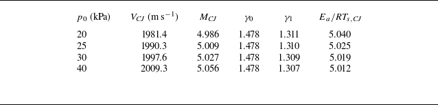
 2
 2
 VCJ
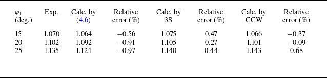
 αm

 φ1
 χ
 1
 μ
 δ

 ε

 LP
 HP
 LO


 1
 2
 p0=40

 S1/λCJ
 Δφ=15∘
 θ2=16.5∘

 θ
 χ


 φ1=15∘
 φ2=30∘

 φ1=15∘
 φ2=30∘
 φ1=20∘
 φ2=35∘

 2
 3
 φ1=15∘
 φ2=30∘


 2
 3
 φ1=20∘
 φ2=35∘

 φ1=15∘
 φ2=30∘
 φ1=20∘
 φ2=35∘

 2

 φ=15∘


 λ
 ε

 λ
 α
 α<1
 b
 b
 Ea/RTs,CJ=5.0
 Ea/RTs,CJ=3.8



