1 Introduction
The singular nature of flow at low Reynolds number (
 $Re$
) has been a topic of immense practical and theoretical interest following the monumental work of Stokes (Reference Stokes1851). The method of perturbation expansions to resolve Stokes’ paradox and Whitehead’s paradox (Whitehead Reference Whitehead1889) by adding inertial effects (Oseen correction) was worked out in detail by Oseen (Reference Oseen1910) and Lamb (Reference Lamb1911) and later by using the method of matched asymptotic expansions by Lagerstrom & Cole (Reference Lagerstrom and Cole1955), Kaplun (Reference Kaplun1957), Kaplun & Lagerstrom (Reference Kaplun and Lagerstrom1957) and Proudman & Pearson (Reference Proudman and Pearson1957). In Stokes’ equations for uniform flow past a sphere, the ratio of the neglected inertia terms to retained viscous terms scales with the distance
 $r$
from the sphere as
 $O(Re(r/R))$
, where
 $R$
is the radius of the sphere, thereby making Stokes’ hypothesis valid for distances less than order
 $R/Re$
(Leal Reference Leal2007). Oseen suggested linearizing the inertial terms instead of neglecting them so that the Navier–Stokes equations become
 $\unicode[STIX]{x1D70C}U_{\infty }\hat{\boldsymbol{\imath }}\boldsymbol{\cdot }\unicode[STIX]{x1D735}\boldsymbol{v}=-\unicode[STIX]{x1D735}p+\unicode[STIX]{x1D707}\unicode[STIX]{x1D6FB}^{2}\boldsymbol{v}$
, where
 $U_{\infty }$
is the velocity of the uniform stream. One of the key ideas that emerges from perturbation analysis (Happel & Brenner Reference Happel and Brenner1965) is that, as long as
 $Re<10$
, only one term in the solution captures the vorticity (a ‘stokeslet’ or an ‘oseenlet’) and that inertial effects vanish only near the body. In this paper, we demonstrate that the presence of heat transfer affects the flow only near the spherical particle. We show that these effects can be captured as steady-state drag and Nusselt-number correlations, which can then be used in large-scale computational simulations of gas–solid flows where it might be expensive to resolve the flow around the particles and where the accuracy of the drag law affects the overall flow behaviour.
Stokes’ solution for creeping flow over a rigid sphere, which is a special case of the Hadamard–Rybczynski solution (Hadamard Reference Hadamard1911; Rybczynski Reference Rybczynski1911), famously demonstrates that the drag force experienced by a sphere of radius
 $R$
in a viscous flow (which is uniform when far away from the sphere) with velocity
 $U_{\infty }$
at steady state has an analytical closed-form solution given by
 $F_{drag}=6\unicode[STIX]{x03C0}\unicode[STIX]{x1D707}_{\infty }U_{\infty }R$
, where
 $\unicode[STIX]{x1D707}_{\infty }$
is the viscosity of the fluid. Henceforth, in this paper, it should be assumed that all drag values are computed at steady state unless otherwise specified. Stokes’ drag is independent of the density of the fluid and assumes that the flow is uniformly at the same temperature and thus has no viscosity variations. When corrected for inertial effects while continuing to assume the absence of temperature variations, the drag experienced by the sphere is higher than Stokes’ drag and all correction terms depend on the fluid density. These inertial corrections also break the fore–aft symmetry in the flow field, which has been experimentally confirmed by Shakespear (Reference Shakespear1914) and Stinberger, Pruppacher & Neiburger (Reference Stinberger, Pruppacher and Neiburger1968). Unlike Stokes’ solution, which is symmetric about the plane at
 $\unicode[STIX]{x1D703}=\unicode[STIX]{x03C0}/2$
, the Oseen flow is asymmetric and that asymmetry is related to the non-zero value of
 $Re$
and increases with an increase in
 $Re$
. For example, Stokes’ streamfunction,
 $\unicode[STIX]{x1D713}(r,\unicode[STIX]{x1D703},\unicode[STIX]{x1D719})$
, for the Oseen equations (Yih Reference Yih1969) is
 $$\begin{eqnarray}\frac{\unicode[STIX]{x1D713}}{UR^{2}}=\frac{(R^{3}+2r^{3})\sin ^{2}\unicode[STIX]{x1D703}}{4R^{2}r}-\frac{3}{Re}(1+\cos \unicode[STIX]{x1D703})(1-\text{e}^{-rRe(1-\cos \unicode[STIX]{x1D703})/4R}).\end{eqnarray}$$
We demonstrate that heating also results in fore–aft asymmetry. For a fixed value of
 $Re$
, the asymmetry increases with an increase in the amount of heat added. Many complete series solutions have been obtained to the Oseen equation in addition to the ones mentioned above, most notably by Goldstein (Reference Goldstein1929) and Van Dyke (Reference Van Dyke1970). Oseen’s correction is, however, an approximation that is valid in a limited range of Reynolds numbers. Semi-empirical modifications of the Oseen equations have been proposed by Lewis & Carrier (Reference Lewis and Carrier1949), while Proudman & Pearson (Reference Proudman and Pearson1957) proposed the method of successive approximations to the Navier–Stokes equations. An elaborate discussion of the method of matched asymptotic expansion applied to this problem can be found in Van Dyke (Reference Van Dyke1964) and Lagerstrom (Reference Lagerstrom1988). Oseen’s correction to Stokes’ drag yields an
 $O(Re)$
correction, which takes the form
 $$\begin{eqnarray}F_{drag}=6\unicode[STIX]{x03C0}\unicode[STIX]{x1D707}_{\infty }U_{\infty }R(1+{\textstyle \frac{3}{16}}Re),\end{eqnarray}$$
while the analysis of Proudman & Pearson (Reference Proudman and Pearson1957) yields
 $$\begin{eqnarray}F_{drag}=6\unicode[STIX]{x03C0}\unicode[STIX]{x1D707}_{\infty }U_{\infty }R(1+{\textstyle \frac{3}{16}}Re+{\textstyle \frac{9}{160}}Re^{2}\ln ({\textstyle \frac{1}{2}}Re)+O(Re^{2})).\end{eqnarray}$$
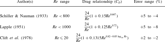
The conventional correlation for the drag on a sphere over the entire range of Reynolds numbers, known as the ‘standard drag curve’, may be found in Lapple (Reference Lapple1951). A large number of theoretical and empirical equations have been proposed to fit this curve. Typically, these correlations attempt to capture the entirety of the Stokes, Oseen and Newton’s law regions and sometimes the region after the point of critical transition. Some notable examples that are popular in the literature are the correlations available from Schiller & Nauman (Reference Schiller and Nauman1933), Lapple (Reference Lapple1951) and Clift & Gauvin (Reference Clift and Gauvin1970). A comprehensive table of available correlations with their associated ranges of deviation may be found as table 5.1 in Clift, Grace & Weber (Reference Clift, Grace and Weber1978). It is clear that there is a compromise between the range of
 $Re$
over which a drag correlation is valid and the error incurred in using the correlation; attempting to capture larger ranges of
 $Re$
results in larger error. Nguyen (Reference Nguyen1973) gives a correlation based on critical examination of available data for spheres where the whole
 $Re$
range has been divided into 10 subintervals with a distinct correlation for each subinterval. These have been obtained by least-squares regression. The correlations may be found in table 5.2 in Clift et al. (Reference Clift, Grace and Weber1978). It is instructive to look at the form of some of these popular correlations noted in table 1. The first term is exactly Stokes drag, which is strictly valid only in the limit
 $Re\rightarrow 0$
. The second term is a ‘correction’ term for inertial effects. As the Reynolds number tends to zero (which can be physically viewed as either a decrease in the speed of the far-field uniform flow or a reduction in the size of the sphere), the correction term decreases faster than Stokes drag and eventually recovers Stokes’ drag exactly. It must be noted that all of these correlations assume that the fluid is at constant density, that the flow is incompressible, and that the fluid is uniformly at the same temperature and thus has no spatial variations in viscosity.
Three popular correlations for the drag on a sphere in uniform flow.

There are no solutions for Stokes’ problem coupled with transfer (heat or mass) which possess the generality of the Hadamard–Rybczynski solution for fluid motion (Clift et al.
Reference Clift, Grace and Weber1978). In order to tackle the problem of heat transfer, the solutions for the velocity of the fluid must be available to solve the energy equation if the flow is incompressible. This becomes even more challenging when either the fluid has variable temperature-dependent density or the fluid is compressible, since the Navier–Stokes equations and the energy equations are coupled and must be solved jointly. Using the matching procedure of Proudman & Pearson (Reference Proudman and Pearson1957) and numerical techniques, the transfer problem has been solved for constant-property fluids most notably by Brenner (Reference Brenner1963) and Masliyah & Epstein (Reference Masliyah and Epstein1972), respectively, among many others. Asymptotic solutions for the Sherwood and Nusselt (
 $Nu$
) numbers have been obtained for the limits of the Péclet number (
 $Pe$
) being either
 $Pe\rightarrow 0$
or
 $Pe\rightarrow \infty$
by Brenner (Reference Brenner1963), Acrivos & Taylor (Reference Acrivos and Taylor1962), Acrivos & Goddard (Reference Acrivos and Goddard1965) and Levich (Reference Levich1962). Specifically, Acrivos & Taylor (Reference Acrivos and Taylor1962) assumed that the velocity field was given by the Stokes solution for slow flow past a sphere and used the method of matched inner and outer expansions to obtain an expression for the mean
 $Nu$
as a function of
 $Pe$
. Of special interest is the study by Kassoy, Adamson & Messiter (Reference Kassoy, Adamson and Messiter1966), who considered heat transfer modifications to compressible low-
 $Re$
flow past a sphere in which significant variations in density occur. The analysis is performed for the cases when
 $\unicode[STIX]{x1D706}=O(1)$
and
 $\unicode[STIX]{x1D706}=O(Re)$
, where
 $\unicode[STIX]{x1D706}=(T_{p}-T_{\infty })/T_{\infty }$
. Here
 $T_{p}$
is the temperature of the sphere while
 $T_{\infty }$
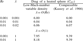
is the temperature of the free stream. Kassoy et al. (Reference Kassoy, Adamson and Messiter1966) show that, for compressible flow at low
 $Re$
,
 $$\begin{eqnarray}C_{D}=\frac{24}{Re}\left[1+Re\left(\frac{3}{16}+\frac{13}{24}\frac{\unicode[STIX]{x1D706}}{Re}\right)\right]+O(Re^{2}\ln Re)\end{eqnarray}$$
if
 $\unicode[STIX]{x1D706}=O(Re)$
while
 $$\begin{eqnarray}C_{D}=\frac{24}{Re}\left[\frac{16C_{2}}{3\unicode[STIX]{x1D706}(\unicode[STIX]{x1D706}+2)}-\frac{\unicode[STIX]{x1D706}(\unicode[STIX]{x1D706}+2)}{3}\right]\end{eqnarray}$$
if
 $\unicode[STIX]{x1D706}=O(1)$
, where the values of
 $C_{2}$
are tabulated in the paper.
The problem of heat transfer from an isothermal sphere in a steady flow at low
 $Re$
when the fluid has constant properties and the fluid is incompressible has been studied by using series expansion by Dennis, Walker & Hudson (Reference Dennis, Walker and Hudson1973) and using numerical techniques by Masliyah & Epstein (Reference Masliyah and Epstein1972). These assumptions imply that the normalized temperature difference (
 $|\unicode[STIX]{x1D706}|$
) must be small in comparison with unity and further that it must be large compared with the square of the Mach number (
 $Ma$
) of the basic flow. Many studies using the method of matched asymptotic expansions (Lagerstrom Reference Lagerstrom1988) that calculate drag coefficients for momentum transfer from bodies at small
 $Re$
and that calculate
 $Nu$
for heat and mass transfer from bodies at small
 $Pe$
are available. The associated problem of heat transfer from spherical droplets has been studied extensively as well; Sazhin (Reference Sazhin2006) reviews many models for heating and evaporation of fuel droplets. Spheres are isotropic bodies and their relative orientation to the free stream does not influence the rate of transfer and thus many attempts have been made to extend solutions for a sphere at low
 $Re$
and low
 $Pe$
to particles of arbitrary shapes (Breach Reference Breach1961; Brenner Reference Brenner1961; Chester Reference Chester1962; Brenner & Cox Reference Brenner and Cox1963). Experimental studies have been performed on the effects of variable properties of fluids on Stokes drag; for example, a strongly temperature-dependent viscosity has been studied by Ansari & Morris (Reference Ansari and Morris1985). Kurose et al. (Reference Kurose, Anami, Fujita and Komori2012) qualitatively study the characteristics of variable-property fluid flow past a heated or cooled sphere for particle Reynolds numbers in the range 50–500 with and without buoyancy and infer that the drag increases with an increase in particle temperature. They do not, however, quantify how the drag varies with particle temperature. Similar studies have also been performed for extremely small particles. Brownian motion of heated nanoparticles has been recently studied by Rings et al. (Reference Rings, Schachoff, Selmke, Cichos and Kroy2010), while the motion of hot particles in viscous fluids has been studied by Oppenheimer, Navardi & Stone (Reference Oppenheimer, Navardi and Stone2016).
It is instructive to ask: How is Stokes’ law for drag modified for a heated sphere in a slow flow? Does the drag increase or decrease? Why? How does fluid buoyancy affect the drag? These are some of the questions motivating the present work. In this paper, we use fully resolved simulations to quantify the effects of heat transfer on the drag of a spatially fixed heated spherical particle held at a fixed temperature at low Reynolds numbers in the range
 $10^{-3}\leqslant Re\leqslant 10$
in a variable-property fluid in the absence of buoyancy and thus attempt to answer the questions posed above. The effects of buoyancy are considered in a subsequent paper. While we have performed some preliminary simulations for cooled spheres, the results and analysis presented in this paper are only for heated spheres.
2 Governing equations and numerical solution
We assume that the heated particle is spherical (with radius
 $R$
, or diameter
 $D=2R$
) and has a prescribed uniform velocity far away from the fixed particle. The fluid has variable density, viscosity and thermal conductivity, which vary only with temperature. For definiteness, consider the initial value problem associated with imposing a particle temperature different from the fluid temperature at
 $t=0$
. The problem is characterized by two regimes: at small times, compressibility effects are important and manifest as an acoustic front (Ganguli Reference Ganguli2018). Following this front, the expected fluid motion occurs at much lower speed. This allows for a low-Mach-number limit (
 $Ma\rightarrow 0$
) formulation of the Navier–Stokes equations (Panton Reference Panton2005), which is the subject of this paper. The Biot number (
 $Bi$
) is the ratio of the conduction resistance to the convection resistance of the particle. The particle is assumed to have a small Biot number (
 $Bi\ll 1$
), which implies that the particle is uniformly at the same temperature and cannot sustain any radial or angular (azimuthal or polar) gradients. This also implies that conduction from the particle to the fluid and convection of the heat thereof is the only mode of heat transfer between the particle and the fluid. The fluid is assumed to be optically thin and, in the absence of other particles, there is no scattered radiation. An order-of-magnitude analysis comparing the heat transfer due to radiation compared to the heat transfer due to convection shows that radiation can be ignored as a mode of heat transfer for the range of particle temperatures considered in this paper. Specifically, even when the particle (assumed to have an emissivity
 $\unicode[STIX]{x1D716}=1$
) temperature is 1200 K and the fluid (air) ambient temperature is 300 K,
 $$\begin{eqnarray}\frac{\unicode[STIX]{x1D716}\unicode[STIX]{x1D70E}_{SB}A(T_{w}^{4}-T_{\infty }^{4})}{hA(T_{w}-T_{\infty })}\approx \frac{1\times \unicode[STIX]{x1D70E}_{SB}(T_{w}^{4}-T_{\infty }^{4})}{2\displaystyle \frac{\unicode[STIX]{x1D705}_{air}}{D}(T_{w}-T_{\infty })}\approx \frac{5.6\times 10^{-8}\times (1200^{4}-300^{4})}{2\times \displaystyle \frac{2\times 10^{-2}}{10^{-6}}\times (1200-300)}=O(10^{-3}).\end{eqnarray}$$
We are interested in the solution when
 $Re$
based on the diameter of the particle is small (
 $O(1)$
and smaller). The creeping-flow limit is of special interest. The numerical solution is obtained by solving the full three-dimensional (3-D) equations. Furthermore, taking the fluid as air, the Prandtl number (
 $Pr$
) of the fluid is close to 1 (specifically
 $Pr\approx 0.7$
). We solve the variable-density low-Mach-number equations (Panton Reference Panton2005; Ham Reference Ham2007) for the fluid, which are
 $$\begin{eqnarray}\displaystyle & \displaystyle {\displaystyle \frac{\unicode[STIX]{x2202}\unicode[STIX]{x1D70C}}{\unicode[STIX]{x2202}t}}+{\displaystyle \frac{\unicode[STIX]{x2202}(\unicode[STIX]{x1D70C}u_{j})}{\unicode[STIX]{x2202}x_{j}}}=0, & \displaystyle\end{eqnarray}$$
 $$\begin{eqnarray}\displaystyle & \displaystyle {\displaystyle \frac{\unicode[STIX]{x2202}(\unicode[STIX]{x1D70C}u_{i})}{\unicode[STIX]{x2202}t}}+{\displaystyle \frac{\unicode[STIX]{x2202}(\unicode[STIX]{x1D70C}u_{i}u_{j})}{\unicode[STIX]{x2202}x_{j}}}=-{\displaystyle \frac{\unicode[STIX]{x2202}p}{\unicode[STIX]{x2202}x_{i}}}+{\displaystyle \frac{\unicode[STIX]{x2202}}{\unicode[STIX]{x2202}x_{j}}}\left(\unicode[STIX]{x1D707}\left({\displaystyle \frac{\unicode[STIX]{x2202}u_{i}}{\unicode[STIX]{x2202}x_{j}}}+{\displaystyle \frac{\unicode[STIX]{x2202}u_{j}}{\unicode[STIX]{x2202}x_{i}}}-{\displaystyle \frac{2}{3}}{\displaystyle \frac{\unicode[STIX]{x2202}u_{k}}{\unicode[STIX]{x2202}x_{k}}}\unicode[STIX]{x1D6FF}_{ij}\right)\right), & \displaystyle\end{eqnarray}$$
 $$\begin{eqnarray}\displaystyle & \displaystyle {\displaystyle \frac{\unicode[STIX]{x2202}(\unicode[STIX]{x1D70C}C_{v}T_{g})}{\unicode[STIX]{x2202}t}}+{\displaystyle \frac{\unicode[STIX]{x2202}(\unicode[STIX]{x1D70C}C_{p}T_{g}u_{j})}{\unicode[STIX]{x2202}x_{j}}}={\displaystyle \frac{\unicode[STIX]{x2202}}{\unicode[STIX]{x2202}x_{j}}}\left(\unicode[STIX]{x1D705}{\displaystyle \frac{\unicode[STIX]{x2202}T_{g}}{\unicode[STIX]{x2202}x_{j}}}\right), & \displaystyle\end{eqnarray}$$
 $$\begin{eqnarray}\displaystyle & \displaystyle P=P_{0}+p=\unicode[STIX]{x1D70C}RT_{g}. & \displaystyle\end{eqnarray}$$
In the above equations,
 $\unicode[STIX]{x1D70C}$
is the fluid density,
 $u_{i}$
is the
 $i$
th component of the fluid velocity vector
 $\boldsymbol{u}$
,
 $p$
is the sum of the hydrostatic and hydrodynamic pressure,
 $P_{0}$
is the thermodynamic pressure,
 $R$
is the ideal gas constant for air,
 $\unicode[STIX]{x1D707}$
is the dynamic viscosity,
 $C_{v}$
is the isochoric specific heat capacity,
 $C_{p}$
is the isobaric specific heat capacity,
 $\unicode[STIX]{x1D705}$
is the thermal conductivity of the fluid, and
 $T_{g}$
is the gas temperature. The total pressure is
 $P$
, where, in the low-Mach-number limit,
 $p\ll P_{0}$
. We will take
 $C_{p}$
and
 $C_{v}$
as constants. Furthermore, in the low-
 $Ma$
limit, the second term of the energy equation includes the pressure work term in addition to the internal energy, which evaluates to the enthalpy and is evaluated as
 $C_{p}T_{g}$
(Panton Reference Panton2005). Also note that, in this limit, heating due to viscous dissipation is negligible (Kundu, Cohen & Dowling Reference Kundu, Cohen and Dowling2014). A power law (Vincenti & Kruger Reference Vincenti and Kruger1965) is used to model the viscosity as a function of temperature. This can be written as
 $\unicode[STIX]{x1D707}=\unicode[STIX]{x1D707}_{0}(T_{g}/T_{\infty })^{n}$
, where
 $\unicode[STIX]{x1D707}$
is the viscosity at temperature
 $T_{g}$
and
 $\unicode[STIX]{x1D707}_{0}$
is the reference viscosity at a temperature
 $T_{\infty }$
. For air, we have
 $\unicode[STIX]{x1D707}_{0}=1.716\times 10^{-5}$
kg m
 $^{-1}$
s
 $^{-1}$
,
 $T_{\infty }=273$
K and
 $n=2/3$
. The variation of thermal conductivity is given by
 $\unicode[STIX]{x1D705}(T_{g})=\unicode[STIX]{x1D707}(T_{g})C_{p}/Pr$
. It must be noted that there are other widely used correlations for the fluid viscosity and thermal conductivity of air in the range of temperature of interest to us. Specifically, other laws may be more accurate at higher temperatures and therefore induce small discrepancies in the drag values reported in this paper at these temperatures. The specific heats and Prandtl number are also functions of temperature, albeit the variations of these quantities in the range of temperature of interest to us are below 10 % and will only result in small discrepancies in the drag values reported in this paper. However, the analysis in this paper that explains the drag modification does not depend on the specific forms of the power laws used.
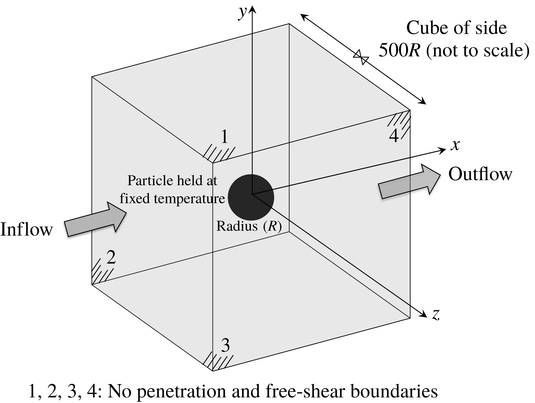
We use the Vida solver to solve the above equations, details of which may be found in Ham (Reference Ham2007). Figure 1 shows a schematic of the numerical set-up, which consists of a sphere of radius
 $R$
held spatially fixed at a fixed temperature inside a cubic box of side
 $500R$
. The size is chosen such that it is appropriate for the
 $Re$
range and particle temperature range that we study to recover more than 99 % of the free-stream velocity. The temperature of the particle is raised from ambient temperature to a fixed temperature over a very short time after which it is held constant. The initial condition for the velocity is uniform
 $x$
-directional flow consistent with the inlet condition, while the density and viscosity fields are set everywhere to equal the ambient values. The system is allowed to evolve in time with the imposed boundary conditions shown in figure 1 until it reaches steady state. At steady state, the convective heat transfer balances the heat flux from the sphere due to the imposed boundary condition. Since the imposed flow at the inlet is uniform and has a prescribed free-stream velocity, and since the particle has a fixed size, this is equivalent to prescribing a far-field
 $Re$
. This
 $Re$
is based on the far-field density and velocity, which are invariant and equal to the initially prescribed values. The mesh on the surface of the particle is structured and is grown outwards until
 $60R$
. This is contained inside a cube of size
 $140R$
. Outside this cube, the mesh is structured while the mesh between the grown spherical mesh and the cube is unstructured but dominated by hexahedral cells for increased accuracy. The governing parameters of the problem are the inflow Reynolds number (
 $Re$
) based on the particle diameter
 $D$
and the Boussinesq parameter (
 $\unicode[STIX]{x1D706}$
) (Lagerstrom Reference Lagerstrom1964; Panton Reference Panton2005) defined as the difference between the particle temperature
 $T_{p}$
and the ambient temperature of the gas
 $T_{\infty }$
normalized by
 $T_{\infty }$
, which are defined as
 $Re=\unicode[STIX]{x1D70C}_{\infty }U_{\infty }D/\unicode[STIX]{x1D707}_{\infty }$
and
 $\unicode[STIX]{x1D706}=(T_{p}-T_{\infty })/T_{\infty }$
, where the subscript
 $\infty$
denotes the values of the parameters in the far field and
 $U_{\infty }$
is the velocity of the fluid specified along the
 $x$
-axis at the inlet. Our study aims to quantify the effect of heat transfer in the absence of gravity on the drag of a heated sphere in the low-
 $Re$
and low-
 $Bi$
regimes. An analysis of the flow of a variable-property fluid including the full effects of temperature variations on the flow is non-trivial and therefore some essential and physical approximations have been made in the literature for studying similar problems.
A schematic of the numerical set-up (not to scale). All contour plots shown in this paper are on the
 $xy$
-plane in the reference frame shown.

In most thermal flow problems with small temperature gradients, a common approximation is the Boussinesq approximation (Boussinesq Reference Boussinesq1903; Spiegel & Veronis Reference Spiegel and Veronis1960). As the amount of heat addition from the sphere to a variable-property fluid increases, the Boussinesq assumption is no longer valid. The simulations performed in this paper solve the fully coupled Navier–Stokes equations and the energy equation and make no assumption about the amount of heat addition from the sphere into the fluid. When heat addition is small, we recover the Boussinesq regime. As the amount of heat addition increases, non-Boussinesq effects start to dominate. The primary quantities of interest are the pressure drag (
 $\boldsymbol{F}_{P}$
), the viscous drag (
 $\boldsymbol{F}_{V}$
) and the Nusselt number (
 $Nu_{D}$
) defined as
 $\boldsymbol{F}_{P}=\oint _{S}(p-p_{\infty })\unicode[STIX]{x1D644}\boldsymbol{\cdot }\boldsymbol{n}\,\text{d}S$
,
 $\boldsymbol{F}_{V}=\oint _{S}\unicode[STIX]{x1D749}\boldsymbol{\cdot }\boldsymbol{n}\,\text{d}S$
and
 $$\begin{eqnarray}Nu_{D}=\frac{hD}{k}=-\frac{D}{A(T_{p}-T_{\infty })}\oint _{S}\unicode[STIX]{x1D735}T\boldsymbol{\cdot }\boldsymbol{n}\,\text{d}S.\end{eqnarray}$$
In the literature, reporting the non-dimensional drag as the coefficient of drag using the inertial scaling is most popular. While adopting this convention, we also report the coefficient of drag using the viscous scaling, since it is the most appropriate scaling given our Reynolds-number range. However, the two are equivalent by a multiplicative constant of
 $Re/4$
. Letting
 $S_{I}=\frac{1}{2}\unicode[STIX]{x1D70C}_{\infty }U_{\infty }^{2}\frac{1}{4}\unicode[STIX]{x03C0}D^{2}$
, the tables herein report the non-dimensional pressure drag (
 $C_{D}^{pres}=|\boldsymbol{F}_{P}|/S_{I}$
), the non-dimensional viscous drag (
 $C_{D}^{visc}=|\boldsymbol{F}_{V}|/S_{I}$
), the inertially scaled coefficient of drag (
 $C_{D}=(|\boldsymbol{F}_{P}+\boldsymbol{F}_{V}|)/S_{I}$
), and the viscously scaled coefficient of drag (
 $C_{DV}=(Re/4)C_{D}$
).
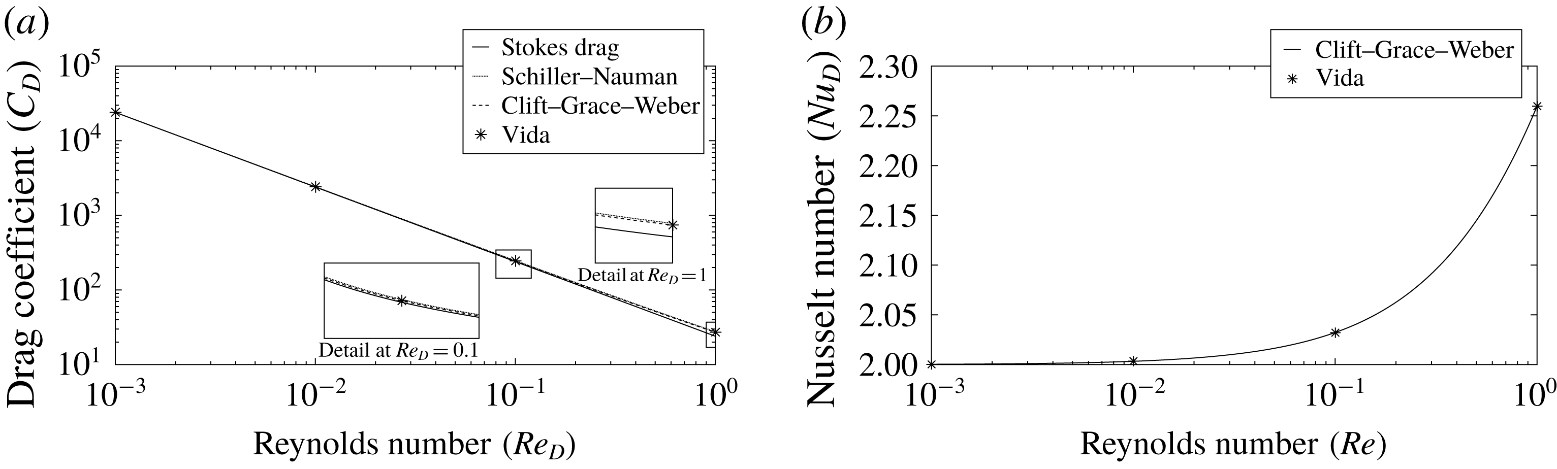
Extensive verification and validation studies have been performed on the code, including grid convergence. Figure 2 shows the numerically obtained drag value and the known analytical form of the drag over four decades of
 $Re$
. We follow within machine precision the correlation in table 5.2, entry B of Clift et al. (Reference Clift, Grace and Weber1978). Contours of the
 $x$
-component of velocity for Reynolds numbers
 $Re=0.01$
and
 $Re=1$
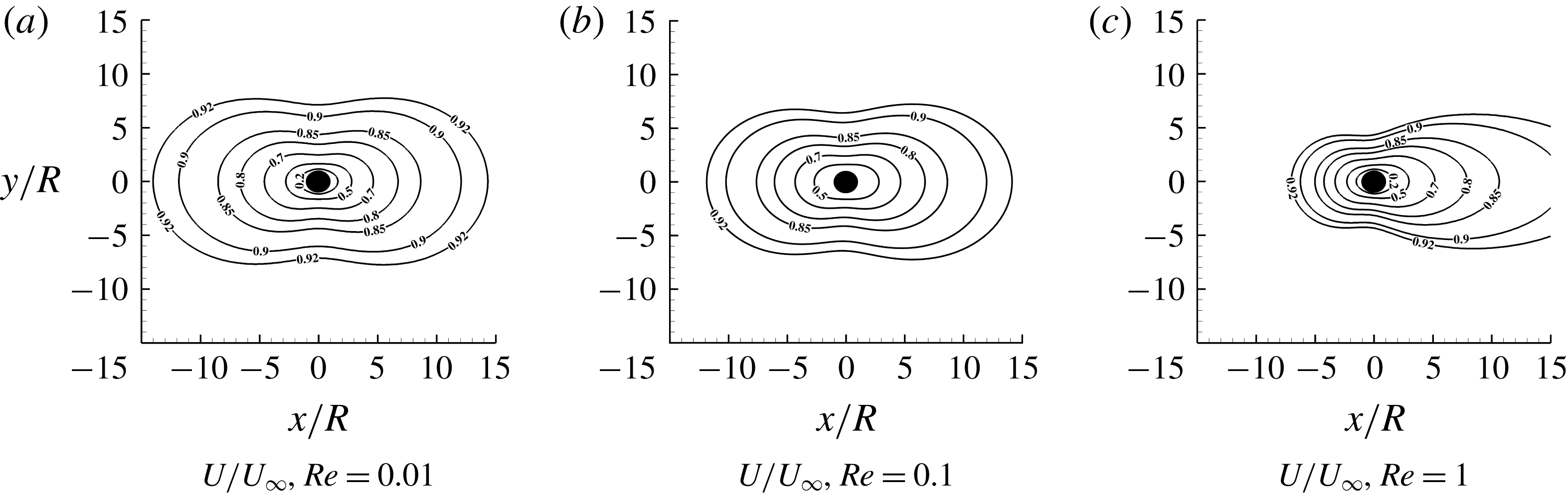
are shown in figure 3. These will help contrast the contours obtained when the particle is heated. Similar contours of pressure and vorticity may be found in Ganguli (Reference Ganguli2018). We also validate the solver by matching the Nusselt number of a sphere at
 $\unicode[STIX]{x1D706}=0$
and at very small
 $\unicode[STIX]{x1D706}$
(
 ${\sim}O(10^{-2})$
) by matching the theoretical prediction of Leal (Reference Leal2007) and the correlation provided in Clift et al. (Reference Clift, Grace and Weber1978). Details of verification and validation studies of the code are documented in Ganguli (Reference Ganguli2018).
Validation of (a) the drag calculation under isothermal conditions and (b) the Nusselt number calculation for very small values of
 $\unicode[STIX]{x1D706}$
(
 $O(10^{-3})$
) over the five decade variation in
 $Re$
of interest in this paper shows good agreement with the correlation of Clift et al. (Reference Clift, Grace and Weber1978). For clarity, the figure shows only
 $Re=0.001$
, 0.01, 0.1 and 1.

Contours of normalized
 $x$
-component of the velocity,
 $U/U_{\infty }$
, for
 $Re=0.01$
, 0.1 and 1 when the particle is not heated (
 $\unicode[STIX]{x1D706}=0$
).

Values of (from left to right per row) the Boussinesq parameter (
 $\unicode[STIX]{x1D706}$
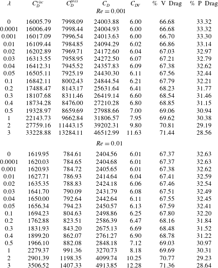
), non-dimensional viscous drag, non-dimensional pressure drag, coefficient of drag with inertial scaling, coefficient of drag with viscous scaling, percentage contribution of viscous drag to the total drag and percentage contribution of pressure drag to the total drag, respectively, at
 $Re=0.001$
and
 $Re=0.01$
reported up to two significant figures after the decimal point.

3 Drag modification of a heated sphere in the absence of gravity
The parameters governing the drag on a heated sphere placed in a uniform flow in the absence of buoyancy are
 $Re$
and
 $\unicode[STIX]{x1D706}$
. Note that
 $\unicode[STIX]{x1D706}$
is a non-dimensional measure of the heat addition from the sphere to the fluid. A parametric study using fully resolved simulations of the heated particle are carried out to obtain the modified component-wise drag and
 $Nu_{D}$
, and is performed over a wide parameter space spanning five decades of
 $Re$
while
 $\unicode[STIX]{x1D706}$
ranges from 0 (isothermal conditions, Stokes’ flow) to 3 (corresponds to the particle temperature being four times the free-stream fluid temperature). Note that
 $\unicode[STIX]{x1D706}\ll 1$
corresponds to the Boussinesq regime where the changes in temperature are small leading to small changes in density. The Boussinesq approximation is valid when
 $\unicode[STIX]{x0394}\unicode[STIX]{x1D70C}/\unicode[STIX]{x1D70C}\ll 1$
. When
 $\unicode[STIX]{x1D706}=0.1$
,
 $\max (\unicode[STIX]{x0394}\unicode[STIX]{x1D70C}/\unicode[STIX]{x1D70C})\sim 10\,\%$
; and when
 $\unicode[STIX]{x1D706}=0.2$
,
 $\max (\unicode[STIX]{x0394}\unicode[STIX]{x1D70C}/\unicode[STIX]{x1D70C})\sim 18\,\%$
. Thus, non-Boussinesq effects become dominant when
 $\unicode[STIX]{x1D706}>0.1$
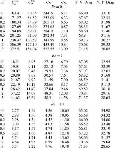
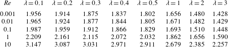
. The computed values of drag are tabulated in tables 2 and 3. Table 4 tabulates the Nusselt (
 $Nu_{D}$
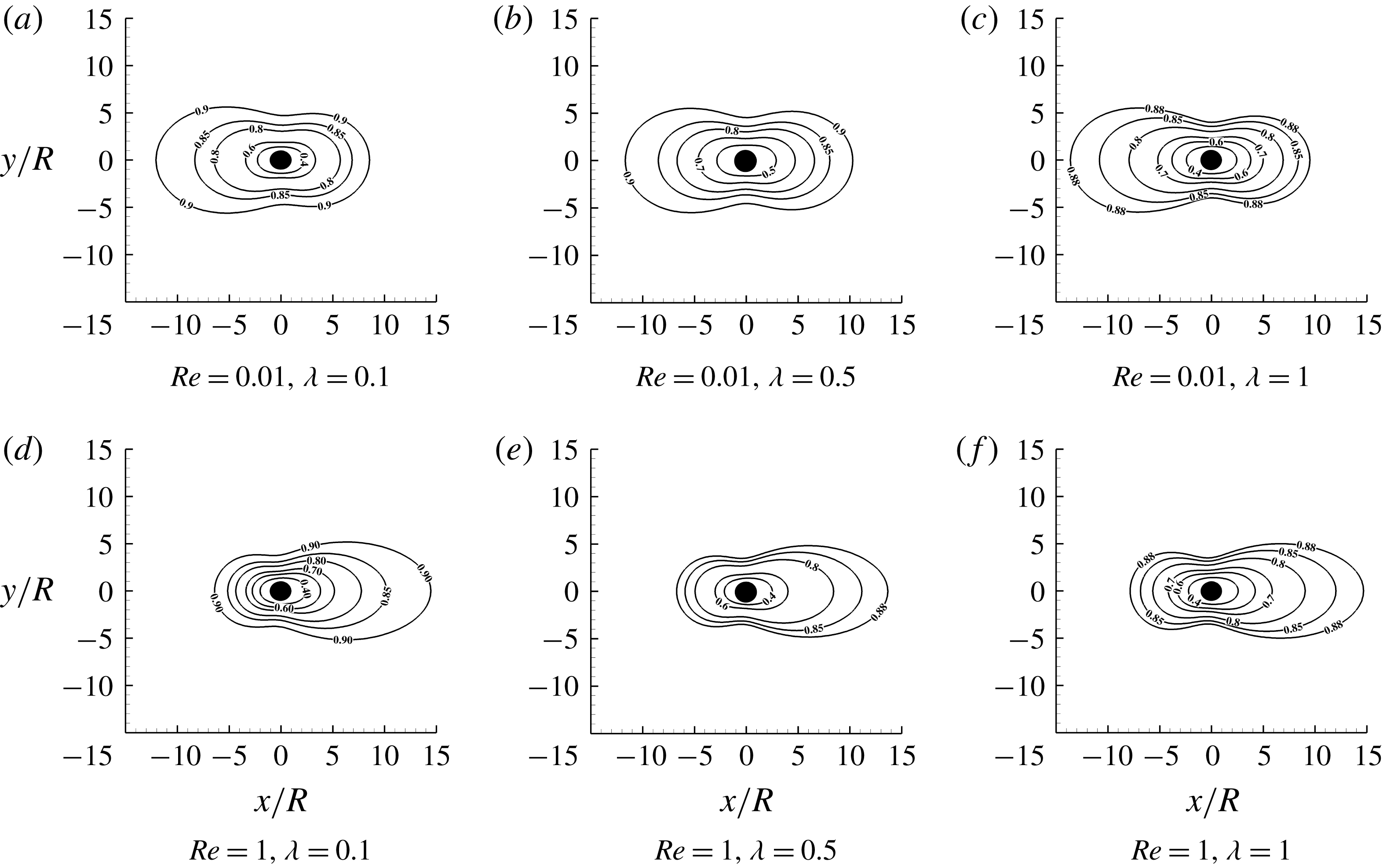
) numbers computed. Appropriately normalized contours of temperature and velocity at two extremes of
 $\unicode[STIX]{x1D706}$
(Boussinesq heating
 $\unicode[STIX]{x1D706}=0.1$
and strongly non-Boussinesq heating
 $\unicode[STIX]{x1D706}=1$
) and two
 $Re$
(
 $Re=0.01$
, where convective effects are small, and
 $Re=1$
, where convective effects are significantly larger) are plotted in figures 5 and 6. Similar plots of contours of density, pressure and vorticity are provided in Ganguli (Reference Ganguli2018).
Values of (from left to right per row) the Boussinesq parameter (
 $\unicode[STIX]{x1D706}$
), non-dimensional viscous drag, non-dimensional pressure drag, coefficient of drag with inertial scaling, coefficient of drag with viscous scaling, percentage contribution of viscous drag to the total drag and percentage contribution of pressure drag to the total drag, respectively, at
 $Re=0.1$
, 1 and 10 reported up to two significant figures after the decimal point.

Values of the Nusselt number based on the diameter of the sphere (
 $Nu_{D}$
) as the Boussinesq parameter (
 $\unicode[STIX]{x1D706}$
) varies from 0 to 3 and the Reynolds number varies from 0.001 to 10.

Let us first draw some qualitative conclusions from the data obtained. At fixed
 $Re$
, the total drag on the particle increases monotonically as
 $\unicode[STIX]{x1D706}$
increases. Similarly, at fixed
 $\unicode[STIX]{x1D706}$
, the total drag on the particle also increases monotonically as
 $Re$
increases. Stokes’ flow yields symmetric velocity fields. When no heat is added, increasing
 $Re$
induces fore–aft asymmetry. When
 $Re$
is fixed and
 $\unicode[STIX]{x1D706}$
is increased, the fore–aft asymmetry becomes more pronounced in comparison to the asymmetry seen at the same
 $Re$
under isothermal conditions (
 $\unicode[STIX]{x1D706}=0$
). Similarly, when
 $\unicode[STIX]{x1D706}$
is fixed and
 $Re$
increases, the fore–aft asymmetry widens as
 $Re$
increases. The difference though is the direction in which the asymmetry arises. Increasing the heat supplied to the fluid by increasing the particle temperature (i.e. higher
 $\unicode[STIX]{x1D706}$
) causes an asymmetry on the anterior stagnation side of the particle, whereas increasing the far-field uniform velocity (i.e. higher
 $Re$
) causes the asymmetry on the posterior stagnation side. Owing to the stagnation region in front of the particle, as
 $\unicode[STIX]{x1D706}$
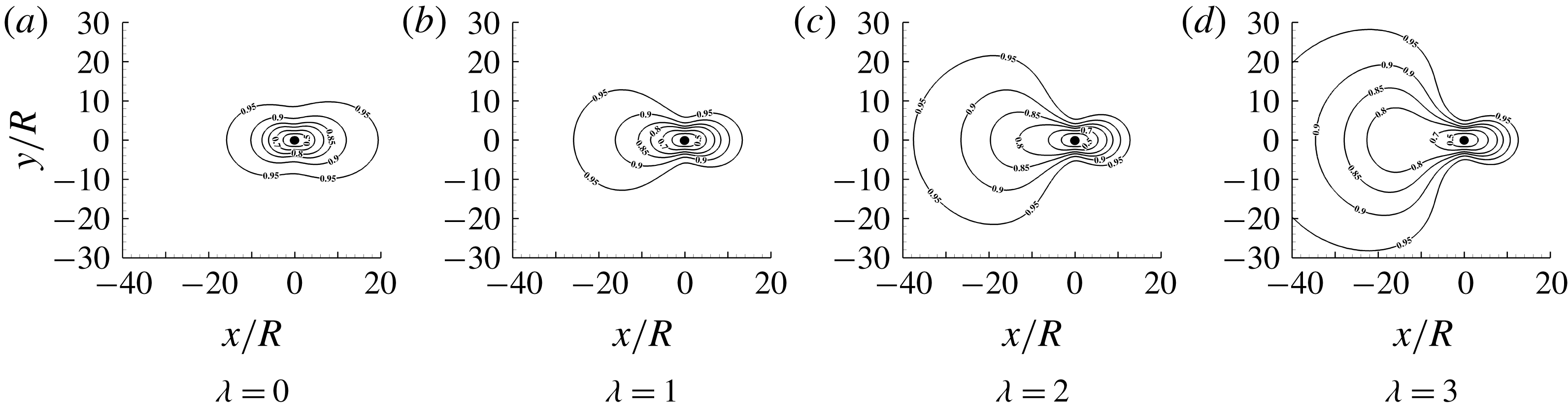
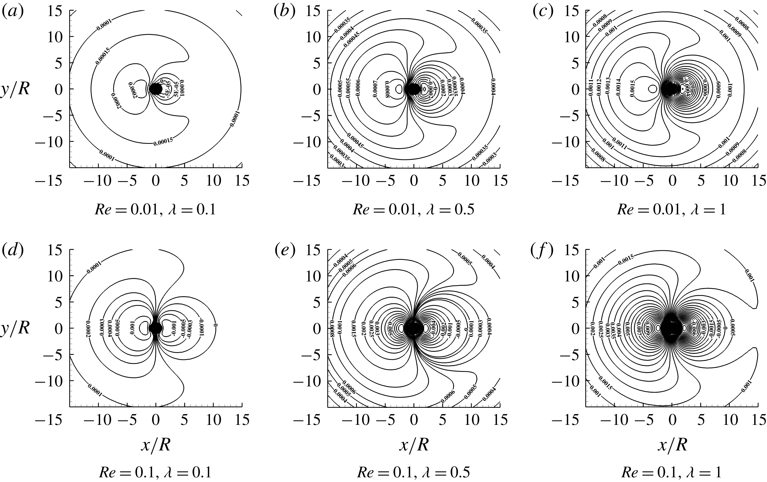
increases, the heat diffusion into the fluid becomes more aggressive. This causes the velocity fields to distort, resulting in the fore–aft asymmetry causing larger velocity gradients, larger pressure drops and a larger viscosity. All of these factors lead to a larger drag on the particle. This fore–aft asymmetry is shown quantitatively for
 $Re=0.1$
(chosen as an example for demonstration) in figure 4 where the contours of the
 $x$
-component of the velocity are plotted for a range of
 $\unicode[STIX]{x1D706}$
values.
It is important to note that the increase in total drag is not dominated by either the pressure or the viscous component of the drag. As can be seen in tables 2 and 3, even though the total increase in drag is large and is dependent on both
 $Re$
and
 $\unicode[STIX]{x1D706}$
, the contribution of the pressure and viscous drag to the total drag changes very little from the canonical ratio of
 $1:2$
obtained analytically in the case of Stokes’ flow. Thus, we infer that there is proportionate increase in both components, leading to an increase in the total drag. Analysing
 $Nu_{D}$
tabulated in 4, at fixed
 $Re$
(equivalent to holding the convective heat transfer constant),
 $Nu_{D}$
decreases as
 $\unicode[STIX]{x1D706}$
increases (equivalent to increasing the conductive heat transfer from the sphere). On the other hand, at fixed
 $\unicode[STIX]{x1D706}$
(equivalent to holding the conductive heat transfer fixed),
 $Nu_{D}$
increases as
 $Re$
increases (equivalent to increasing the convective heat transfer). On analysing the resultant temperature fields at
 $Re$
approaching Stokes’ limit (
 $Re=0.001$
,
 $0.01$
), we can make an important observation: despite the fore–aft asymmetry in the velocity field which strengthens as
 $\unicode[STIX]{x1D706}$
increases, the temperature field remains close to spherical (the eccentricity increase with respect to the isothermal case (
 $\unicode[STIX]{x1D706}=0$
) is approximately 7 % when
 $\unicode[STIX]{x1D706}=1$
). The density mimics this behaviour since in the low-Mach-number limit, the total pressure is almost constant and dominated by the thermodynamic pressure, and thus the temperature and density are inversely related. This is not the case, however, as the
 $Re$
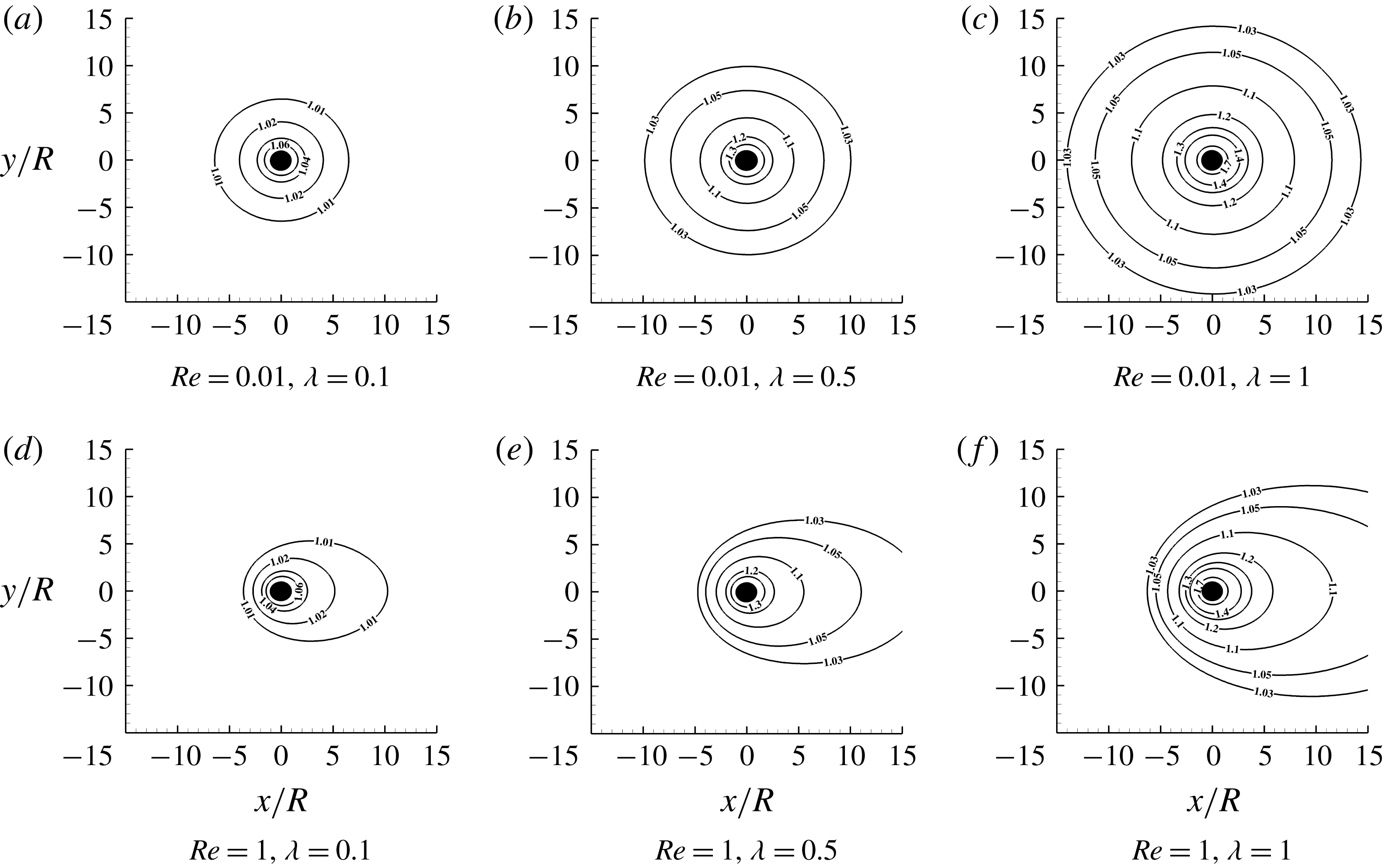
number increases. This difference is clearly demonstrated in figure 5. The small eccentricity in the temperature contours when
 $Re$
is small is caused due to the Oseen correction terms (small convective corrections) in the absence of which we would be solving a simple heat equation with spherically symmetric boundary conditions yielding exactly spherical contours. The Stokes–Oseen correction is important for
 $r\sim O(R/Re)$
, also known as the Oseen distance. This suggests that the density, temperature and velocity fields can be expanded in the form of a perturbation expansion with the base solution being the Stokes–Oseen solution. In the Stokes–Oseen limit, the flow around the heated sphere can be thought of as a deviation from constant-density Stokes–Oseen flow around an unheated sphere for the velocity field and a heat diffusion problem with Oseen correction terms for the density and temperature fields – the deviation being the result of mass rebalancing due to the variable density and variable properties of the fluid.
Normalized contours of the
 $x$
-component of the velocity,
 $U/U_{\infty }$
, for
 $Re=0.1$
and a range of Boussinesq parameters
 $\unicode[STIX]{x1D706}=0$
, 1, 2 and 3. The fore–aft asymmetry becomes more pronounced as the heat addition from the particle to the fluid increases due to an increase in
 $\unicode[STIX]{x1D706}$
.

Contours of normalized temperature,
 $T/T_{\infty }$
, for
 $Re=0.01$
(a–c) and
 $Re=1$
(d–f), each for three cases of
 $\unicode[STIX]{x1D706}$
- one with low heat addition (
 $\unicode[STIX]{x1D706}=0.1$
), one with moderate heat addition (
 $\unicode[STIX]{x1D706}=0.5$
), and one with large heat addition (
 $\unicode[STIX]{x1D706}=1$
). The corresponding contours of
 $\unicode[STIX]{x1D70C}/\unicode[STIX]{x1D70C}_{\infty }$
can be derived from the above figures by using (2.5).

Contours of the normalized
 $x$
-component of velocity,
 $U/U_{\infty }$
, for
 $Re=0.01$
(a–c) and
 $Re=1$
(d–f), each for three cases of the Boussinesq parameter: one with low heat addition (
 $\unicode[STIX]{x1D706}=0.1$
), one with moderate heat addition (
 $\unicode[STIX]{x1D706}=0.5$
), and one with large heat addition (
 $\unicode[STIX]{x1D706}=1$
).

3.1 Importance of volume expansion in gases
Let us first quantify the role played by volume expansion of the fluid when heat addition is present. Consider the general form of the equation of state
 $\unicode[STIX]{x1D70C}=\unicode[STIX]{x1D70C}(p,T)$
. This leads to
 $$\begin{eqnarray}\displaystyle {\displaystyle \frac{1}{\unicode[STIX]{x1D70C}}}{\displaystyle \frac{\text{D}\unicode[STIX]{x1D70C}}{\text{D}t}}=\left({\displaystyle \frac{1}{\unicode[STIX]{x1D70C}}}\frac{\unicode[STIX]{x2202}\unicode[STIX]{x1D70C}}{\unicode[STIX]{x2202}p}\bigg|_{T}\right){\displaystyle \frac{\text{D}p}{\text{D}t}}-\left(-{\displaystyle \frac{1}{\unicode[STIX]{x1D70C}}}{\displaystyle \frac{\unicode[STIX]{x2202}\unicode[STIX]{x1D70C}}{\unicode[STIX]{x2202}T}}\bigg|_{p}\right){\displaystyle \frac{\text{D}T}{\text{D}t}}=\unicode[STIX]{x1D6FC}{\displaystyle \frac{\text{D}p}{\text{D}t}}-\unicode[STIX]{x1D6FD}{\displaystyle \frac{\text{D}T}{\text{D}t}}. & & \displaystyle\end{eqnarray}$$
Here,
 $\unicode[STIX]{x1D6FC}$
is the isothermal compressibility coefficient of the fluid while
 $\unicode[STIX]{x1D6FD}$
is the bulk expansion coefficient (or thermal expansion coefficient) of the fluid. Transforming this equation using viscous scaling of the variables and noting that the scaling of time
 $t$
does not matter in our analysis, we introduce
 $\unicode[STIX]{x1D70C}^{\ast }=\unicode[STIX]{x1D70C}/\unicode[STIX]{x1D70C}_{\infty }$
,
 $\unicode[STIX]{x1D6FD}^{\ast }=\unicode[STIX]{x1D6FD}/\unicode[STIX]{x1D6FD}_{\infty }$
,
 $\unicode[STIX]{x1D6FC}^{\ast }=\unicode[STIX]{x1D6FC}/\unicode[STIX]{x1D6FC}_{\infty }$
,
 $p^{\ast }=p/(\unicode[STIX]{x1D707}_{\infty }U_{\infty }/D)$
,
 $t^{\ast }=t/t_{ref}$
, and
 $T^{\ast }=(T-T_{\infty })/(T_{p}-T_{\infty })=(T-T_{\infty })/\unicode[STIX]{x1D706}T_{\infty }$
, to get
 $$\begin{eqnarray}\displaystyle {\displaystyle \frac{1}{\unicode[STIX]{x1D70C}^{\ast }}}{\displaystyle \frac{\text{D}\unicode[STIX]{x1D70C}^{\ast }}{\text{D}t^{\ast }}}=\left({\displaystyle \frac{\unicode[STIX]{x1D707}_{\infty }U_{\infty }\unicode[STIX]{x1D6FC}_{\infty }}{D}}\right)\unicode[STIX]{x1D6FC}^{\ast }{\displaystyle \frac{\text{D}p^{\ast }}{\text{D}t^{\ast }}}-(\unicode[STIX]{x1D6FD}_{\infty }\unicode[STIX]{x1D706}T_{\infty })\unicode[STIX]{x1D6FD}^{\ast }{\displaystyle \frac{\text{D}T^{\ast }}{\text{D}t^{\ast }}}. & & \displaystyle\end{eqnarray}$$
Noting that the speed of sound in an ideal gas is
 $c_{\infty }=\sqrt{\unicode[STIX]{x1D6FE}_{\infty }p_{\infty }/\unicode[STIX]{x1D70C}_{\infty }}$
, the isothermal compressibility can be used along with the ideal gas law,
 $p_{\infty }=\unicode[STIX]{x1D70C}_{\infty }RT_{\infty }$
(
 $R$
being the specific gas constant), to derive
 $\unicode[STIX]{x1D6FC}_{\infty }=(1/\unicode[STIX]{x1D70C}_{\infty })(\unicode[STIX]{x2202}\unicode[STIX]{x1D70C}/\unicode[STIX]{x2202}p)_{T_{\infty }}=1/(\unicode[STIX]{x1D70C}_{\infty }RT_{\infty })$
implying
 $c_{\infty }^{2}=\unicode[STIX]{x1D6FE}_{\infty }RT_{\infty }=\unicode[STIX]{x1D6FE}_{\infty }/\unicode[STIX]{x1D70C}_{\infty }\unicode[STIX]{x1D6FC}_{\infty }$
. Then,
 $\unicode[STIX]{x1D6FD}_{\infty }\unicode[STIX]{x1D706}T_{\infty }\gg \unicode[STIX]{x1D707}_{\infty }U_{\infty }\unicode[STIX]{x1D6FC}_{\infty }/D$
if
 $$\begin{eqnarray}\displaystyle \left({\displaystyle \frac{\unicode[STIX]{x1D6FD}_{\infty }\unicode[STIX]{x1D706}T_{\infty }}{\unicode[STIX]{x1D6FE}_{\infty }}}\right)\left({\displaystyle \frac{\unicode[STIX]{x1D70C}_{\infty }U_{\infty }D}{\unicode[STIX]{x1D707}_{\infty }}}\right)\gg {\displaystyle \frac{\unicode[STIX]{x1D6FC}_{\infty }U_{\infty }^{2}\unicode[STIX]{x1D70C}_{\infty }}{\unicode[STIX]{x1D6FE}_{\infty }}}={\displaystyle \frac{U_{\infty }^{2}}{c_{\infty }^{2}}}\quad \;\Longrightarrow \;\quad Re\left({\displaystyle \frac{\unicode[STIX]{x1D6FD}_{\infty }\unicode[STIX]{x1D706}T_{\infty }}{\unicode[STIX]{x1D6FE}_{\infty }}}\right)\gg Ma^{2}.\qquad & & \displaystyle\end{eqnarray}$$
Note that this scaling holds when
 $\unicode[STIX]{x1D706}\neq 0$
. Since
 $\unicode[STIX]{x1D6FE}_{\infty }=O(1)$
and if
 $\unicode[STIX]{x1D706}ReT_{\infty }$
is fixed and
 $T_{\infty }=283$
K, then
 $\unicode[STIX]{x1D6FD}_{\infty }\approx 3.55\times 10^{-3}$
(K
 $^{-1}$
) for air, while it is approximately
 $8.88\times 10^{-5}$
(K
 $^{-1}$
) for water, which is approximately 44 times smaller. Even though this is a specific example, the trend of
 $\unicode[STIX]{x1D6FD}_{\infty }$
being larger for gases than liquids holds. In a recent remarkable and significant paper, Oppenheimer et al. (Reference Oppenheimer, Navardi and Stone2016) used the Lorentz reciprocal theorem and perturbation analysis to analytically study the motion of hot particles in a viscous liquid at very low
 $Re$
(e.g. Brownian motion of hot nanoscopic particles) and low
 $Pe$
by accounting for viscosity variations while assuming incompressibility of the fluid. Their study is the first to derive analytical expressions for the force and the torque on an arbitrarily shaped, translating and rotating particle in this regime. The error incurred due to the assumption of incompressibility in such a scenario is small, as is shown by the scaling analysis above. However, for larger particles in gases like air, the correction due to volume expansion of the fluid is significant and non-negligible, as is evidenced by our simulations. The results are presented in terms of a small parameter
 $\unicode[STIX]{x1D716}=((T_{p}-T_{\infty })/\unicode[STIX]{x1D707}_{0})(\text{d}\unicode[STIX]{x1D707}/\text{d}T)|_{T_{\infty }}$
with a sign that depends on the behaviour of the viscosity distribution with temperature. For example, in ideal gases,
 $\text{d}\unicode[STIX]{x1D707}/\text{d}T>0$
, while in common liquids
 $\text{d}\unicode[STIX]{x1D707}/\text{d}T<0$
. The analysis that follows this section will inherit this characteristic due to the temperature-dependent viscosity in the momentum equation. In other words, if the prescribed viscosity variation in our solver had the characteristic that
 $\text{d}\unicode[STIX]{x1D707}/\text{d}T<0$
, we would observe a corresponding decrease of drag with increasing temperature. Our simulations corroborate Oppenheimer et al.’s (Reference Oppenheimer, Navardi and Stone2016) assumption that distortions induced by the flow on the temperature field can be neglected in the regime when
 $Pe$
is very small, which corresponds to
 $Re\ll 1$
and
 $\unicode[STIX]{x1D706}\ll 1$
as is shown in figure 5. Owing to this assumption, in addition to assuming constant-density incompressibility of the fluid, it is sufficient for Oppenheimer et al. (Reference Oppenheimer, Navardi and Stone2016) to solve
 $\unicode[STIX]{x1D735}\boldsymbol{\cdot }\boldsymbol{u}=0$
and
 $-\unicode[STIX]{x1D735}p+\unicode[STIX]{x1D735}\boldsymbol{\cdot }(2\unicode[STIX]{x1D707}\unicode[STIX]{x1D64E})=-\unicode[STIX]{x1D735}p+\unicode[STIX]{x1D707}\unicode[STIX]{x1D6FB}^{2}\boldsymbol{u}+(\unicode[STIX]{x1D735}\unicode[STIX]{x1D707})\boldsymbol{\cdot }[\unicode[STIX]{x1D735}\boldsymbol{u}+(\unicode[STIX]{x1D735}\boldsymbol{u})^{\text{T}}]=0$
, where
 $\unicode[STIX]{x1D64E}$
is the rate-of-strain tensor given by
 $\unicode[STIX]{x1D64E}=\frac{1}{2}(\unicode[STIX]{x1D735}\boldsymbol{u}+(\unicode[STIX]{x1D735}\boldsymbol{u})^{\text{T}})$
, thereby assuming that temperature-induced density variations,
 $\unicode[STIX]{x0394}\unicode[STIX]{x1D70C}$
, do not significantly affect the flow. However, in the case of interest to us, where (3.3) is true,
 $\unicode[STIX]{x1D6FD}_{\infty }\unicode[STIX]{x1D706}T_{\infty }=O(1)$
and
 $Re(\unicode[STIX]{x1D6FD}_{\infty }\unicode[STIX]{x1D706}T_{\infty }/\unicode[STIX]{x1D6FE}_{\infty })\gg Ma^{2}$
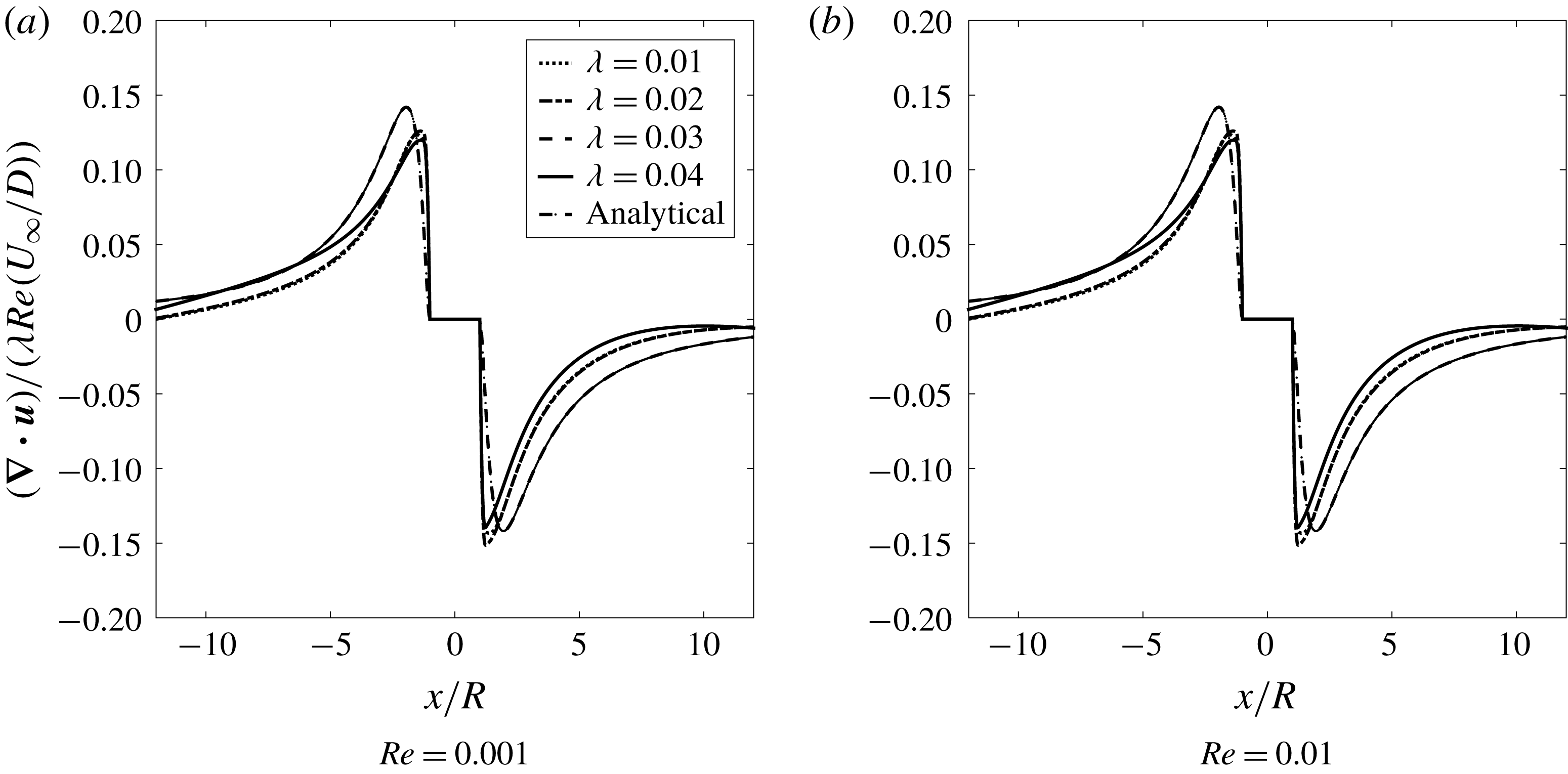
, we must include variable-density effects. Figure 11 shows a comparison of the rate of dilatation for different values of
 $\unicode[STIX]{x1D706}$
at two values of
 $Re=0.01$
and
 $0.1$
. It can be seen that the effects of variable density are more pronounced as
 $Re$
and
 $\unicode[STIX]{x1D706}$
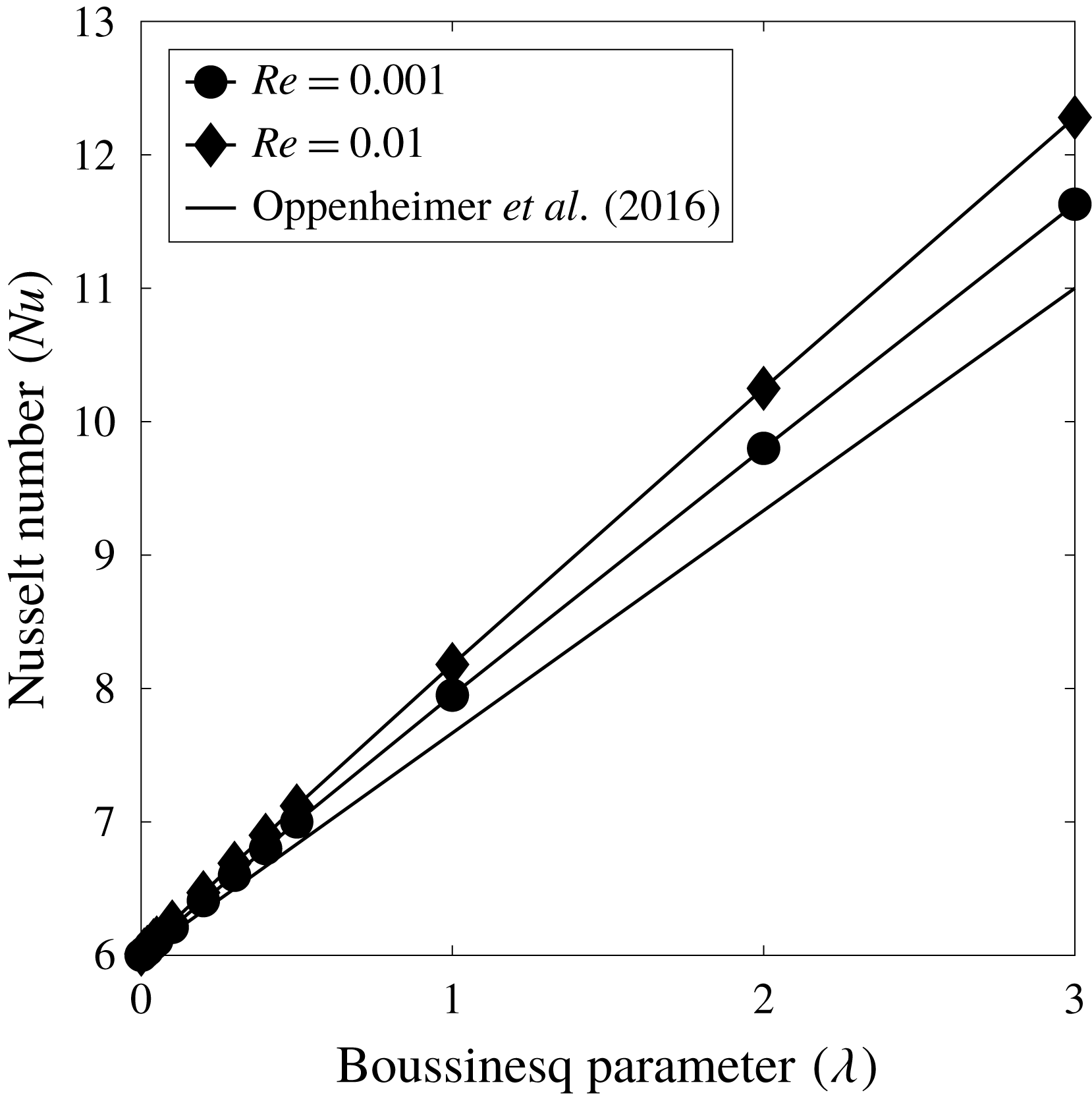
increase. In figure 7, we show a comparison between the numerically obtained drag and the drag that is predicted by the Oppenheimer–Navardi–Stone (Oppenheimer et al.
Reference Oppenheimer, Navardi and Stone2016) first-order drag correction
 $F_{drag}=6\unicode[STIX]{x03C0}\unicode[STIX]{x1D707}_{\infty }RU_{\infty }(1+\frac{5}{12}\unicode[STIX]{x1D716})+O(\unicode[STIX]{x1D716})$
. This correlation evaluates to
 $F_{drag}=6\unicode[STIX]{x03C0}\unicode[STIX]{x1D707}_{\infty }RU_{\infty }(1+\frac{10}{36}\unicode[STIX]{x1D706})$
following the notation in this paper.
Comparison of the analytically predicted drag modification from Oppenheimer et al. (Reference Oppenheimer, Navardi and Stone2016) and the observed drag modification from numerical simulations presented in table 2.

3.2 An explanation of drag modification due to heating as
 $Re\rightarrow 0$

Clearly, when the quantity
 $Re(\unicode[STIX]{x1D6FD}_{\infty }\unicode[STIX]{x1D706}T_{\infty }/\unicode[STIX]{x1D6FE}_{\infty })$
is not small, variable-density effects are important. To account for this and inspired by Oppenheimer et al. (Reference Oppenheimer, Navardi and Stone2016), we derive a set of equations simpler than the full Navier–Stokes equations that help explain the large modification in drag by leveraging the results from our numerical simulations. This formulation should not be thought of as a complete and independent problem in itself but rather as a physical explanation for the sources of the observed drag enhancement in the presence of heat addition in ideal gases. The near-sphericity of the temperature field suggests that the convective terms in the energy equation take the form of linearized Oseen-like correction terms. The proposed simplification couples the energy equation with the continuity and momentum equations only via the convective Oseen correction terms. Since the fully resolved simulations solve the full Navier–Stokes equations (2.2)–(2.5) in three dimensions, we have the computed (true) values of the scalar and vector fields at all points in the domain at steady state. The simplified set of equations at steady state are
 $$\begin{eqnarray}\displaystyle & \displaystyle \unicode[STIX]{x1D735}\boldsymbol{\cdot }(\unicode[STIX]{x1D70C}\boldsymbol{u})=0, & \displaystyle\end{eqnarray}$$
 $$\begin{eqnarray}\displaystyle & \displaystyle \unicode[STIX]{x1D70C}U_{\infty }\hat{\boldsymbol{\imath }}\boldsymbol{\cdot }\unicode[STIX]{x1D735}\boldsymbol{u}=-\unicode[STIX]{x1D735}p+\unicode[STIX]{x1D735}\boldsymbol{\cdot }\unicode[STIX]{x1D749}, & \displaystyle\end{eqnarray}$$
 $$\begin{eqnarray}\displaystyle & \displaystyle \unicode[STIX]{x1D70C}C_{p}U_{\infty }\hat{\boldsymbol{\imath }}\boldsymbol{\cdot }\unicode[STIX]{x1D735}T=\unicode[STIX]{x1D735}\boldsymbol{\cdot }(\unicode[STIX]{x1D705}\unicode[STIX]{x1D735}T) & \displaystyle\end{eqnarray}$$
 $p=\unicode[STIX]{x1D70C}RT$
is the equation of state, and
 $\unicode[STIX]{x1D749}=\unicode[STIX]{x1D707}(\unicode[STIX]{x1D735}\boldsymbol{u}+(\unicode[STIX]{x1D735}\boldsymbol{u})^{\text{T}}-\frac{2}{3}(\unicode[STIX]{x1D735}\boldsymbol{\cdot }\boldsymbol{u})\unicode[STIX]{x1D644})$
is the stress tensor, with
 $\unicode[STIX]{x1D644}$
the identity tensor and
 $\unicode[STIX]{x1D707}$
the dynamic viscosity. These equations are the variable-density form of the Oseen approximation. They could be solved numerically and are expected to yield accurate results when
 $Re\ll 1$
. Heat addition to a variable-property fluid results in a non-zero rate of dilatation (contour plots shown in figure 11 as a function of
 $Re$
and
 $\unicode[STIX]{x1D706}$
) in the near-vicinity of the hot particle in order to satisfy mass conservation. This may be interpreted as ‘mass rebalancing’ of the fluid near the hot particle. At fixed
 $\unicode[STIX]{x1D706}$
, the spatial extent where
 $\unicode[STIX]{x1D735}\boldsymbol{\cdot }\boldsymbol{u}\neq 0$
grows as
 $Re$
increases. At a fixed
 $Re$
, the spatial extent where
 $\unicode[STIX]{x1D735}\boldsymbol{\cdot }\boldsymbol{u}\neq 0$
grows as
 $\unicode[STIX]{x1D706}$
increases. These figures further corroborate the assumption in Oppenheimer et al. (Reference Oppenheimer, Navardi and Stone2016) that at very small
 $Re$
(at an order of magnitude analysed in Oppenheimer et al. (Reference Oppenheimer, Navardi and Stone2016)), the spatial extent where the rate of dilatation is non-zero is so small that the fluid may be assumed to be incompressible without incurring a large error. The regime in which Oppenheimer et al. (Reference Oppenheimer, Navardi and Stone2016) carry out their analysis corresponds to the case where the change in drag of a hot particle from the value when the particle is at the same temperature as the fluid may be solely attributed to the change in viscosity as a function of temperature; this is equivalent to assuming that the terms
 $-(1/\unicode[STIX]{x1D70C})(\boldsymbol{u}\boldsymbol{\cdot }\unicode[STIX]{x1D735}\unicode[STIX]{x1D70C})\approx 0$
and
 $\unicode[STIX]{x1D70C}U_{\infty }\hat{\boldsymbol{\imath }}\boldsymbol{\cdot }\unicode[STIX]{x1D735}\boldsymbol{u}\approx 0$
everywhere in the fluid.
In what follows, we show that the change in drag of a hot particle from the isothermal value of drag is explained well by adding a suitable irrotational and dilatational velocity field to the Stokes–Oseen flow. We seek a perturbation solution of (3.4) in the limit of small temperature (implies small density) variations and write (denoting Stokes–Oseen by the suffix SO)
 $\unicode[STIX]{x1D70C}=\unicode[STIX]{x1D70C}_{\infty }(1+\unicode[STIX]{x1D706}\unicode[STIX]{x1D70C}^{(1)}+\unicode[STIX]{x1D706}^{2}\unicode[STIX]{x1D70C}^{(2)}+\cdots \,)$
,
 $T=T_{\infty }(1+\unicode[STIX]{x1D706}T^{(1)}+\unicode[STIX]{x1D706}^{2}T^{(2)}+\cdots \,)$
and
 $\boldsymbol{u}=\boldsymbol{u}_{SO}+\unicode[STIX]{x1D706}\boldsymbol{u}^{(1)}+\unicode[STIX]{x1D706}^{2}\boldsymbol{u}^{(2)}+\cdots \,$
. At first order (
 $O(\unicode[STIX]{x1D706})$
), the fluid continuity equation becomes
 $\unicode[STIX]{x1D735}\boldsymbol{\cdot }\boldsymbol{u}^{(1)}=-(\unicode[STIX]{x1D735}\unicode[STIX]{x1D70C}^{(1)}\boldsymbol{\cdot }\boldsymbol{u}_{SO})$
. Mass rebalancing is solely due to density differentials that are produced when there are temperature differentials. We can represent the modified velocity field as a correction to the Stokes–Oseen velocity field, which itself can be rewritten as the Helmholtz sum of a rotational and irrotational component that correspond to a scalar potential
 $\unicode[STIX]{x1D719}$
and a vector potential
 $\boldsymbol{A}$
as
 $\boldsymbol{u}=\boldsymbol{u}_{SO}+\unicode[STIX]{x1D735}\unicode[STIX]{x1D719}+\unicode[STIX]{x1D735}\times \boldsymbol{A}=\boldsymbol{u}_{SO}+\unicode[STIX]{x1D706}\boldsymbol{u}^{(1)}$
. The rotational correction has been described in detail in Oppenheimer et al. (Reference Oppenheimer, Navardi and Stone2016). As will be seen from our analysis, we are able to recover a significant portion (more than 90 %) of the drag modification by accounting for only the irrotational correction. Thus,
 $\boldsymbol{u}\approx \boldsymbol{u}_{mod}=\boldsymbol{u}_{SO}+\unicode[STIX]{x1D735}\unicode[STIX]{x1D719}$
. The canonical approach to solving a problem using a perturbation expansion is to obtain the partial differential equations and the boundary conditions at each order of
 $\unicode[STIX]{x1D706}$
and solve them successively. The above approximation allows us to partially bypass this process. The irrotational part captures the correction to the velocity field to conserve mass when the flow changes due to heat addition. Taking the divergence of this approximation and recognizing that the Stokes–Oseen solution is divergence-free yields
 $$\begin{eqnarray}\displaystyle \unicode[STIX]{x1D6FB}^{2}\unicode[STIX]{x1D719}\approx \unicode[STIX]{x1D706}(\unicode[STIX]{x1D735}\boldsymbol{\cdot }\boldsymbol{u}^{(1)})=-\unicode[STIX]{x1D706}(\unicode[STIX]{x1D735}\unicode[STIX]{x1D70C}^{(1)}\boldsymbol{\cdot }\boldsymbol{u}_{SO}). & & \displaystyle\end{eqnarray}$$
In the low-
 $Re$
or the Stokes–Oseen limit, the contribution from the higher-order expansion terms in the perturbation expansion is small. The true solutions to
 $\unicode[STIX]{x1D70C}$
,
 $T$
and
 $\boldsymbol{u}$
are already known from the fully resolved simulations. Thus, as
 $\unicode[STIX]{x1D706}\rightarrow 0$
, we have that
 $\unicode[STIX]{x1D70C}^{(1)}\approx (\unicode[STIX]{x1D70C}-\unicode[STIX]{x1D70C}_{\infty })/\unicode[STIX]{x1D706}$
, where
 $\unicode[STIX]{x1D70C}$
is the density that is known from the simulations.
An analytical expression for
 $\boldsymbol{u}_{SO}$
is known. We solve the Poisson equation (3.5) to obtain
 $\unicode[STIX]{x1D719}$
. On the surface of the sphere, we impose a no-penetration boundary condition which is equivalent to imposing a Neumann boundary condition. Far away from the sphere, the velocity correction goes to zero as the velocity field becomes the imposed uniform velocity field. Thus, equation (3.5) is subject to
 $\unicode[STIX]{x1D735}\unicode[STIX]{x1D719}\boldsymbol{\cdot }\hat{\boldsymbol{r}}=0$
if
 $r=R$
and
 $\unicode[STIX]{x1D735}\unicode[STIX]{x1D719}=0$
as
 $r\rightarrow \infty$
, where
 $r$
is the radial coordinate centred at the centre of the sphere and
 $\hat{\boldsymbol{r}}$
is the unit vector normal to the sphere. Since we are solving a Poisson equation with Neumann boundary conditions, the obtained solution
 $\unicode[STIX]{x1D719}$
is unique up to a constant; its value does not affect the rest of the solution. Calculating
 $\unicode[STIX]{x1D735}\unicode[STIX]{x1D719}$
yields the approximation to the modified velocity field denoted by
 $\boldsymbol{u}_{mod}=\boldsymbol{u}_{SO}+\unicode[STIX]{x1D735}\unicode[STIX]{x1D719}$
. On substituting this modified velocity in the momentum equation, we obtain an equation for the approximation to the modified hydrodynamic pressure, denoted as
 $p_{mod}$
. Taking the divergence of both sides of this equation yields a Poisson equation for
 $p^{(1)}$
(where
 $p_{mod}=p_{SO}(1+\unicode[STIX]{x1D706}p^{(1)}+\cdots \,)$
), which can be solved with appropriate boundary conditions. The equation at
 $O(\unicode[STIX]{x1D706})$
for
 $p^{(1)}$
is
 $$\begin{eqnarray}\displaystyle -p_{\infty }\unicode[STIX]{x1D6FB}^{2}p^{(1)}=\unicode[STIX]{x1D735}\boldsymbol{\cdot }(\unicode[STIX]{x1D70C}_{\infty }U_{\infty }\hat{\boldsymbol{\imath }}\boldsymbol{\cdot }\unicode[STIX]{x1D735}\boldsymbol{u}^{(1)}+\unicode[STIX]{x1D70C}_{\infty }\unicode[STIX]{x1D70C}^{(1)}U_{\infty }\hat{\boldsymbol{\imath }}\boldsymbol{\cdot }\unicode[STIX]{x1D735}\boldsymbol{u}_{SO}-\unicode[STIX]{x1D735}\boldsymbol{\cdot }\unicode[STIX]{x1D749}^{(1)})=\unicode[STIX]{x1D735}\boldsymbol{\cdot }\unicode[STIX]{x1D733}(\boldsymbol{x}), & & \displaystyle\end{eqnarray}$$
where
 $\unicode[STIX]{x1D749}=\unicode[STIX]{x1D749}_{SO}+\unicode[STIX]{x1D706}\unicode[STIX]{x1D749}^{(1)}$
and is subject to the boundary conditions
 $-p_{\infty }\unicode[STIX]{x1D735}p^{(1)}\boldsymbol{\cdot }\hat{\boldsymbol{r}}=\unicode[STIX]{x1D733}(\boldsymbol{x})\boldsymbol{\cdot }\hat{\boldsymbol{r}}$
if
 $r=R$
and
 $p^{(1)}=0$
if
 $r\rightarrow \infty$
. It must also be noted that, since
 $\unicode[STIX]{x1D70C}$
is obtained from the numerical solution and fully known, the temperature field is also known due to the equation of state. Now
 $\boldsymbol{u}_{mod}$
and
 $p_{mod}$
can be used to calculate the viscous, pressure and total drag on the sphere, which can be compared to the values obtained from the full 3-D solver.
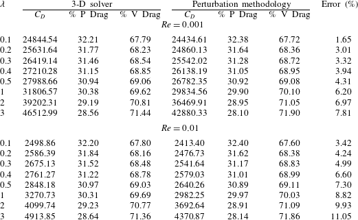
Comparison of the total drag and its components (pressure (P Drag) and viscous (V Drag) components) computed using the 3-D solver with those computed from the perturbation methodology as a function of
 $\unicode[STIX]{x1D706}$
at
 $Re=0.001$
and
 $0.01$
. The last column shows the error incurred in the perturbation approach compared to the 3-D solver.

The results of this low-Mach-number perturbation analysis are tabulated for the range of Boussinesq parameters
 $\unicode[STIX]{x1D706}$
under study at
 $Re=0.001$
and
 $Re=0.01$
in table 5, which compares the total coefficient of drag and its components obtained from solving the full 3-D Navier–Stokes equations to that obtained from the perturbation approach. We see that the perturbation approach recovers the true drag to within 10 % error even when
 $\unicode[STIX]{x1D706}$
is as large as 2 and strong non-Boussinesq effects are present. To develop a physical sense of the magnitude of heat supplied, consider the case when the ambient temperature of the gas is 300 K. The value
 $\unicode[STIX]{x1D706}=2$
corresponds to a particle temperature of 900 K. The Stokes–Oseen solution is obtained as a linearized approximation to the Navier–Stokes equations. As
 $\unicode[STIX]{x1D706}$
increases, the heat addition into the fluid increases causing strong density gradients, which increases the nonlinear coupling of the momentum and energy equations. As these nonlinearities rise, the explanation power of the linear model decreases. With the perturbation methodology, the drag decomposition maintains the approximate ratio of the pressure and viscous drag of
 $1:2$
consistent with the numerical solution. This further vindicates the physical validity of the perturbation methodology in the low-
 $Re$
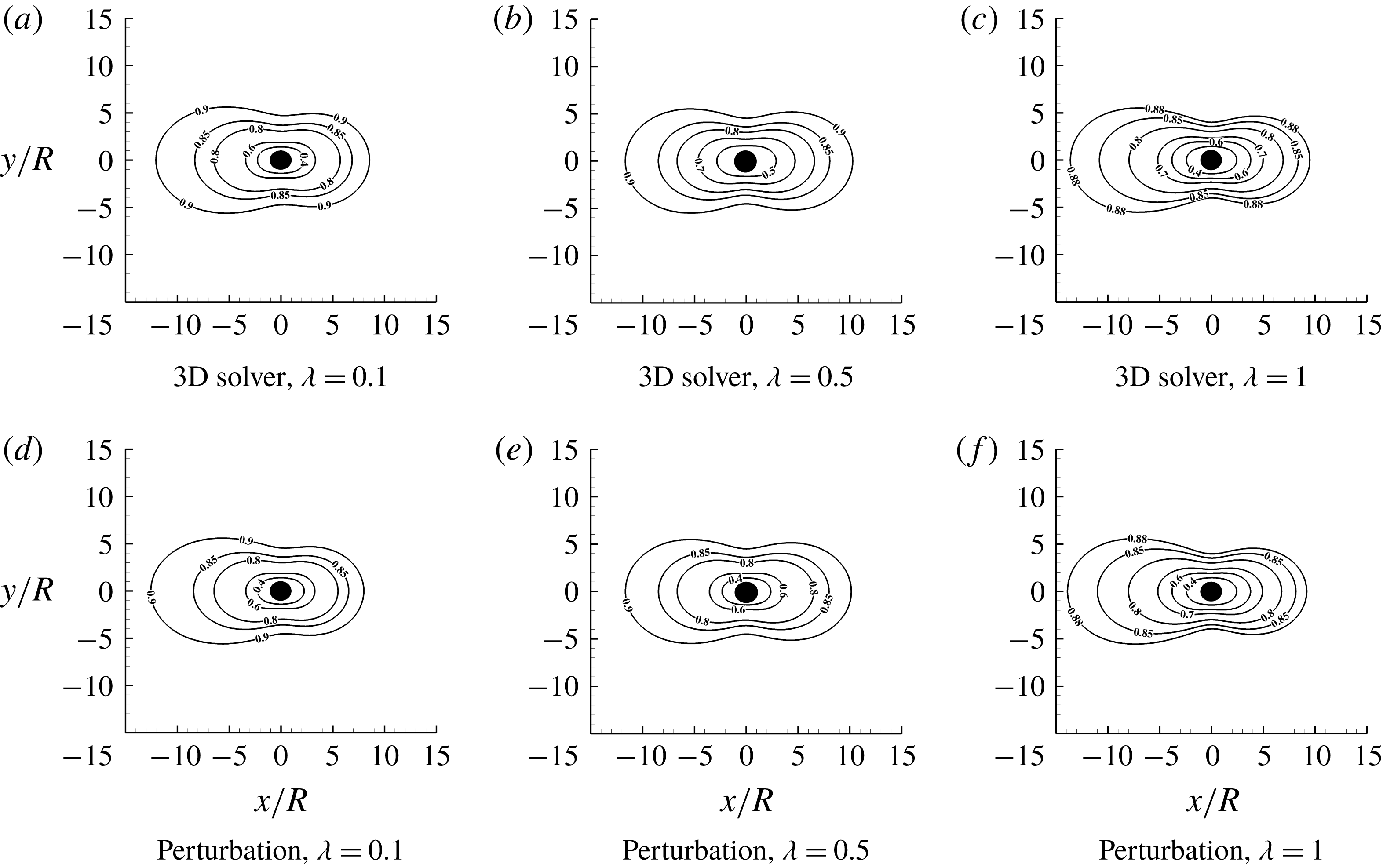
limit. Comparison of the velocity contours resulting from the full 3-D solver and the contours resulting from the perturbation methodology is shown for two cases of
 $Re$
and
 $\unicode[STIX]{x1D706}$
in figure 8. Just as with drag, better agreement is seen at lower
 $Re$
and lower
 $\unicode[STIX]{x1D706}$
when the reduced equations are a good approximation to the nonlinear coupled equations. At higher Reynolds numbers, this approach fails to recover the drag even at very small
 $\unicode[STIX]{x1D706}$
due to the presence of nonlinear terms which cannot be neglected.
Comparison of normalized
 $x$
-velocity,
 $U/U_{\infty }$
, contours resulting from the 3-D solver (a–c) and the contours resulting from the perturbation methodology (d–f), each for three cases of the Boussinesq parameter: one with low heat addition (
 $\unicode[STIX]{x1D706}=0.1$
), one with moderate heat addition (
 $\unicode[STIX]{x1D706}=0.5$
), and one with large heat addition (
 $\unicode[STIX]{x1D706}=1$
), for
 $Re=0.01$
.

3.3 Suggested correlations for
$C_{D}$
and
$Nu_{D}$
via least-squares regression


The explanation of the observed drag modification as the effect of an irrotational correction to the Stokes–Oseen solution due to mass rebalancing and the effect of the fluid’s variable properties is encouraging. This approach is also consistent with the form of the correlations for the drag coefficient of a sphere at low Reynolds numbers in the literature as seen in Oseen (Reference Oseen1910), Goldstein (Reference Goldstein1929), Chester, Breach & Proudman (Reference Chester, Breach and Proudman1969), Chester et al. (Reference Chester, Breach and Proudman1969) and others stated in tables 3.1 and 5.1 in Clift et al. (Reference Clift, Grace and Weber1978), where the first term of the correlation is Stokes’ drag (independent of inertial effects and hence independent of the density of the fluid) and the subsequent terms account for inertial corrections to the Stokes’ drag and is a function of the density of the fluid. As
 $Re\rightarrow O(1)$
, inertial effects begin to become significant and the correction terms account for this effect. Inspired by the observations from our perturbation analysis and in order to collapse the data obtained from the parametric numerical study over the
 $\unicode[STIX]{x1D706}$
and
 $Re$
ranges studied in this paper (
 $10^{-3}\leqslant Re\leqslant 10$
,
 $0\leqslant \unicode[STIX]{x1D706}\leqslant 3$
), we seek a drag correlation composed of two terms: a first term that resembles the Stokes–Oseen drag (and thus uses non-dimensional parameters defined at the ambient fluid temperature) and a correction term that captures the mass rebalance due to the variable density of the fluid caused by the heating of the sphere (which uses non-dimensional parameters defined at an appropriate temperature, which is a hyper-parameter to be found by tuning). Taking inspiration from the correlations in table 5.1 in Clift et al. (Reference Clift, Grace and Weber1978), we model the second term to be of power-law form. We use all the data from the fully resolved simulations of the full 3-D Navier–Stokes equations over the two parameters
 $Re$
and
 $\unicode[STIX]{x1D706}$
. Statistical methods of feature selection and hypothesis testing are used to choose the optimal form of the power-law terms in the nonlinear regression procedure, while hold-out cross-validation is used to choose between multiple hypotheses (Vapnik Reference Vapnik1998). The regression has multiple hyper-parameters that must be chosen; for example, the density and viscosity used to define the Reynolds number used in the correction terms (denoted as the film temperature Reynolds number (
 $Re_{T_{film}}$
)) can be evaluated at film temperatures which are a linear combination of
 $T_{p}$
and
 $T_{\infty }$
. A full description of the process of building these accurate correlations along with the algorithm used to tune the hyper-parameters is described in Ganguli (Reference Ganguli2018).
The Clift–Grace–Weber correlation (Clift et al.
Reference Clift, Grace and Weber1978), valid for
 $Re\leqslant 20$
and stated in table 1, is extended to take the form
 $C_{D}=C_{D}^{CGW}+\unicode[STIX]{x1D6FC}\unicode[STIX]{x1D706}^{\unicode[STIX]{x1D6FD}}Re_{T_{film}}^{\unicode[STIX]{x1D6FE}}$
. The adjusted-
 $R^{2}$
is used as the metric to evaluate these regression fits. The best fit to the data is obtained when
 $Re_{T_{film}}=\unicode[STIX]{x1D70C}_{\infty }U_{\infty }D/\unicode[STIX]{x1D707}(T_{film})$
and
 $T_{film}=T_{\infty }$
. It has an adjusted-
 $R^{2}$
value of 99.56 % and the values of the hyper-parameters along with their 95 % confidence intervals are
 $\unicode[STIX]{x1D6FC}=10.7672\pm 0.0416$
,
 $\unicode[STIX]{x1D6FD}=0.9673\pm 0.0130$
and
 $\unicode[STIX]{x1D6FE}=-0.9529\pm 0.0095$
. Thus the correlation for the drag of a heated sphere when
 $10^{-3}\leqslant Re\leqslant 10$
with the definitions of the hyper-parameters defined above is
 $$\begin{eqnarray}\displaystyle C_{D}={\displaystyle \frac{24}{Re}}(1+0.1315Re^{0.82-0.05\log _{10}Re})+10.7672\unicode[STIX]{x1D706}^{0.9673}Re^{-0.9529}. & & \displaystyle\end{eqnarray}$$
A feature ablation study reveals that if the feature
 $\unicode[STIX]{x1D706}^{\unicode[STIX]{x1D6FD}}$
is left out, the best adjusted-
 $R^{2}$
drops to 57.70 %. If the feature
 $Re_{T_{film}}^{\unicode[STIX]{x1D6FE}}$
is left out, the adjusted-
 $R^{2}$
drops to a paltry 13.58 %. Rewritten in terms of
 $C_{DV}$
, the correlation becomes
 $$\begin{eqnarray}\displaystyle C_{DV}=6(1+0.1315Re^{0.82-0.05\log _{10}Re})+2.6918\unicode[STIX]{x1D706}^{0.9673}Re^{0.0471}. & & \displaystyle\end{eqnarray}$$
(As observed in (3.8), the exponent of
 $\unicode[STIX]{x1D706}$
is
 ${\approx}1$
and the exponent of
 $Re$
is
 ${\approx}0$
. This, and the insight from § 3.2 that the drag modification can be captured quite well with a linear perturbation expansion in
 $\unicode[STIX]{x1D706}$
, suggests an alternative correlation for
 $C_{DV}$
of a heated particle with an additive correction
 $\unicode[STIX]{x1D6FC}_{M}\unicode[STIX]{x1D706}$
. Linear regression on the data from tables 3 and 4 reveals the representation of the best fit as
 $C_{DV}=6(1+0.1315Re^{0.82-0.05\log _{10}Re})+2.3801\unicode[STIX]{x1D706}$
with an adjusted-
 $R^{2}$
value of 96.08 %. The 95 % confidence interval on this coefficient is
 $\unicode[STIX]{x1D6FC}_{M}=2.3801\pm 0.0423$
.)
It is worth mentioning that when
 $\unicode[STIX]{x1D706}=0$
, the correlations for drag in (3.7) and (3.8) reduce to the Clift–Grace–Weber correlation. A similar approach is used to derive a correlation for the Nusselt number from the data in table 4. When the velocity is everywhere zero (which is the case when
 $Re\rightarrow 0$
) and the temperature difference between the fluid and sphere is small (
 $\unicode[STIX]{x1D706}<O(10^{-2})$
), diffusion of heat is in the radial direction only and thus
 $Nu_{D}=2$
. From the work of Brenner (Reference Brenner1963) and Masliyah & Epstein (Reference Masliyah and Epstein1972), we know that for
 $\unicode[STIX]{x1D706}\rightarrow 0$
and very small
 $Re$
,
 $Nu_{D}$
approaches 2, while for large
 $Re$
,
 $Nu_{D}$
becomes proportional to
 $Re^{1/3}$
. The neglected convection terms are not negligible far away from the sphere since the ratio of convective to diffusive terms is
 $O(Re(r/a))$
. Asymptotic solutions are available for
 $Nu_{D}$
using the matching procedure of Proudman & Pearson (Reference Proudman and Pearson1957). Analogous to the Oseen correction for drag, Brenner (Reference Brenner1963) suggests that for small
 $\unicode[STIX]{x1D706}$
, we have
 $\frac{1}{2}Nu-1=\frac{1}{4}Re$
as
 $Re\rightarrow 0$
and is accurate to
 $O(Re)$
. Acrivos & Taylor (Reference Acrivos and Taylor1962) extended this to higher-order terms with only slight improvement. Clift et al. (Reference Clift, Grace and Weber1978) state that for small
 $\unicode[STIX]{x1D706}$
,
 $Nu_{D}=1+(1+Re)^{1/3}$
, which is valid for all
 $Re$
in creeping flow within 2 % error. This may be more generally written (Clift et al.
Reference Clift, Grace and Weber1978) as
 $Nu_{D}=1+(1+Pe)^{1/3}$
, where
 $Pe=RePr$
. This correlation is extended to take the form (Ganguli Reference Ganguli2018),
 $Nu_{D}=[1+(1+Re)^{1/3}]\text{e}^{-\unicode[STIX]{x1D6FC}\unicode[STIX]{x1D706}-\unicode[STIX]{x1D6FD}\unicode[STIX]{x1D706}^{2}-\unicode[STIX]{x1D6FE}(Re-Re_{T_{film}})}$
, where
 $\unicode[STIX]{x1D6FC}$
,
 $\unicode[STIX]{x1D6FD}$
,
 $\unicode[STIX]{x1D6FE}$
and
 $T_{film}$
are the hyper-parameters. The statistical procedure outlined in Ganguli (Reference Ganguli2018) yields the optimal definition of
 $Re_{T_{film}}$
for the drag correlation to be
 $Re_{T_{film}}=\unicode[STIX]{x1D70C}_{\infty }U_{\infty }D/\unicode[STIX]{x1D707}(T_{film})$
such that
 $T_{film}$
is
 $T_{film}=0.080T_{p}+0.920T_{\infty }$
. The best fit has an adjusted-
 $R^{2}$
value of 97.59 %. If, instead, the conventional definition of the film temperature is used, i.e.
 $T_{film}=0.5(T_{p}+T_{\infty })$
, the fit has an adjusted-
 $R^{2}$
of
 ${\sim}97.05\,\%$
. It must be noted that the correlations proposed here depend on the specific form of the power law used, and using other power laws may induce discrepancies that may surmount this small difference in the values of adjusted-
 $R^{2}$
. We will therefore use the conventional definition of
 $T_{film}$
. The values of the hyper-parameters along with their 95 % confidence intervals are
 $\unicode[STIX]{x1D6FC}=0.2201\pm 0.0082$
,
 $\unicode[STIX]{x1D6FD}=-0.0331\pm 0.0005$
and
 $\unicode[STIX]{x1D6FE}=-0.0046\pm 0.0001$
. A feature ablation study reveals that if the feature
 $\text{e}^{\unicode[STIX]{x1D6FC}\unicode[STIX]{x1D706}}$
is suppressed by setting
 $\unicode[STIX]{x1D6FC}=0$
, the adjusted-
 $R^{2}$
drops to 56.59 %. Suppressing
 $\text{e}^{\unicode[STIX]{x1D6FD}\unicode[STIX]{x1D706}^{2}}$
by setting
 $\unicode[STIX]{x1D6FD}=0$
yields an adjusted-
 $R^{2}$
of 91.24 %. Suppressing
 $\text{e}^{\unicode[STIX]{x1D6FE}(Re-Re_{T_{film}})}$
by setting
 $\unicode[STIX]{x1D6FE}=0$
yields an adjusted-
 $R^{2}$
of 95.94 %. Thus the correlation for the Nusselt number of a heated sphere becomes
 $$\begin{eqnarray}\displaystyle Nu_{D}=[1+(1+Re)^{1/3}]\text{e}^{-0.2201\unicode[STIX]{x1D706}+0.0331\unicode[STIX]{x1D706}^{2}+0.0046(Re-Re_{T_{film}})} & & \displaystyle\end{eqnarray}$$
when
 $10^{-3}\leqslant Re\leqslant 10$
.
In both of the above correlations, the value of
 $\unicode[STIX]{x1D707}$
is obtained from the power law for viscosity stated in § 2. It is worth mentioning that, when
 $\unicode[STIX]{x1D706}=0$
, the correlation for
 $Nu_{D}$
in (3.9) reduces to the Clift–Grace–Weber correlation for
 $Nu_{D}$
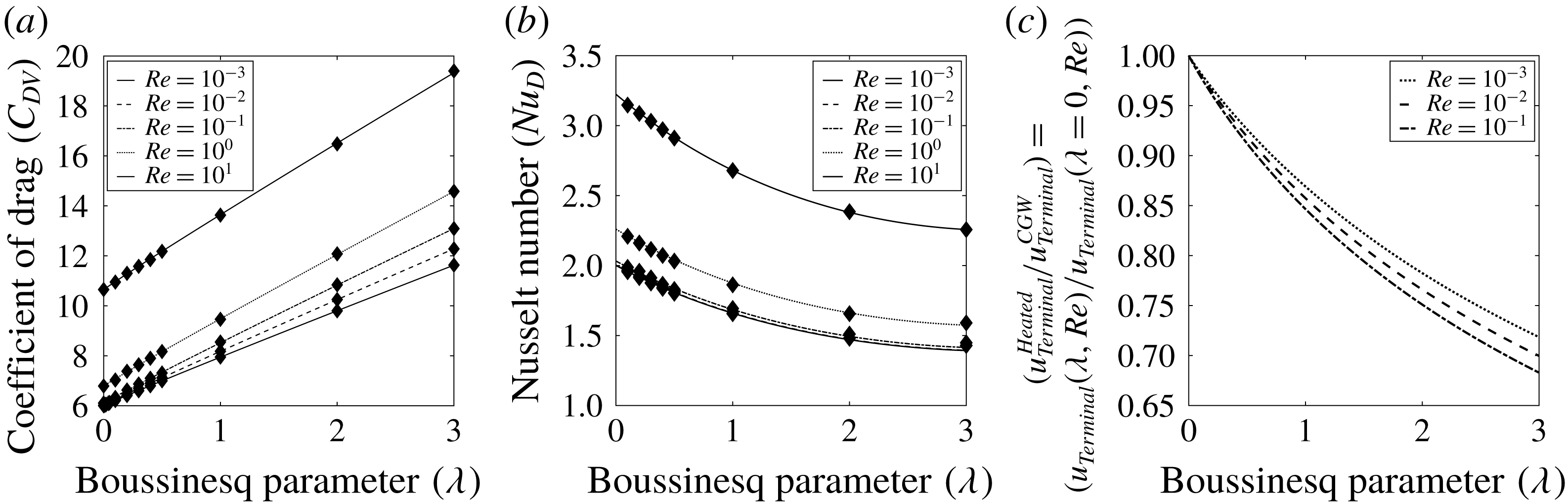
. Figure 9 shows the performance of the inferred correlations for drag and the Nusselt number. Figure 9(a) shows the plot of the drag correlation while figure 9(b) shows the plot of the Nusselt number correlation as a function of
 $\unicode[STIX]{x1D706}$
for the five decades of
 $Re$
. The correlations are plotted as lines and the values obtained from the particle-resolved simulations are plotted as filled diamonds. Since these correlations have been inferred from simulations of fixed particles, they do not include the effect of mobility of particles. However, we expect our correlations to hold as long as a particle moves at nearly constant velocity. One way to measure the impact of the drag correlation is to measure its effect on the terminal velocity of a hot particle falling due to gravity in a fluid, starting at rest. If the fluid density is
 $\unicode[STIX]{x1D70C}_{f}$
, particle density is
 $\unicode[STIX]{x1D70C}_{p}$
, particle volume is
 $V$
, acceleration due to gravity is
 $g$
, particle diameter is
 $D$
, time is
 $t$
and particle velocity is
 $u$
, the equation governing the falling particle is
 $$\begin{eqnarray}\unicode[STIX]{x1D70C}_{p}V\frac{\text{d}u}{\text{d}t}=(\unicode[STIX]{x1D70C}_{p}-\unicode[STIX]{x1D70C}_{f})Vg-\frac{3V\unicode[STIX]{x1D70C}_{f}}{4D}u^{2}C_{D}.\end{eqnarray}$$
(For metal particles (e.g. nickel) falling in air,
 $\unicode[STIX]{x1D70C}_{p}\gg \unicode[STIX]{x1D70C}_{f}$
, so that the influence of temperature on the density ratio
 $\unicode[STIX]{x1D70C}_{f}/\unicode[STIX]{x1D70C}_{p}$
can be safely ignored for the analysis shown here. Justifiably, we can also assume zero or negligibly small contributions from fluid inertia, added mass and Basset–Boussinesq history terms in the Maxey–Riley–Gatignol equation. When
 $Re\ll 1$
, the added-mass factor is
 $\unicode[STIX]{x1D6FD}=3\unicode[STIX]{x1D70C}_{f}/(\unicode[STIX]{x1D70C}_{f}+2\unicode[STIX]{x1D70C}_{p})\ll 1$
.)
At steady state, we have
 $$\begin{eqnarray}u^{2}C_{D}=\left(1-\frac{\unicode[STIX]{x1D70C}_{f}}{\unicode[STIX]{x1D70C}_{p}}\right)g\left(\frac{4\unicode[STIX]{x1D70C}_{p}D}{3\unicode[STIX]{x1D70C}_{f}}\right).\end{eqnarray}$$
If
 $\unicode[STIX]{x1D70C}_{f}$
,
 $\unicode[STIX]{x1D70C}_{p}$
,
 $g$
and
 $D$
are constant, then
 $u_{terminal}^{2}C_{D}$
is a constant, allowing us to obtain the ratio of the terminal velocity of a hot particle (
 $u_{terminal}^{heated}$
) and the terminal velocity of an unheated particle (
 $u_{terminal}^{CGW}$
) as
 $u_{terminal}^{heated}/u_{terminal}^{CGW}=\sqrt{C_{D}^{CGW}/C_{D}^{heated}}$
. This ratio is plotted as a function of
 $\unicode[STIX]{x1D706}$
for
 $Re=0.001$
, 0.01 and 0.1 in figure 9(c).
Performance of the suggested correlations for (a)
 $C_{DV}$
and (b)
 $Nu_{D}$
stated in (3.8) and (3.9), respectively, as a function of
 $Re$
and
 $\unicode[STIX]{x1D706}$
. Lines denote correlations and diamonds denote simulation results. (c) The ratio of the terminal velocity of a heated particle to an unheated particle falling under gravity starting from rest.

3.4 A scaling for the rate of dilatation for
$\unicode[STIX]{x1D706}\rightarrow 0$
and
$Re\rightarrow 0$


We saw in previous sections that when
 $Re(\unicode[STIX]{x1D6FD}_{\infty }\unicode[STIX]{x1D706}T_{\infty }/\unicode[STIX]{x1D6FE}_{\infty })\gg Ma^{2}$
,
 $\unicode[STIX]{x1D6FD}_{\infty }\unicode[STIX]{x1D706}T_{\infty }=O(1)$
and
 $(\unicode[STIX]{x1D707}_{\infty }U_{\infty }\unicode[STIX]{x1D6FC}_{\infty })/D\ll 1$
, we must include variable-density effects. These effects result in a finite rate of dilatation. In this section, we analytically derive a scaling for the rate of dilatation (
 $\unicode[STIX]{x1D701}$
) in the limit of
 $Re\rightarrow 0$
and
 $\unicode[STIX]{x1D706}\rightarrow 0$
. Following the analysis in Leal (Reference Leal2007), assuming
 $\unicode[STIX]{x1D705}$
and
 $\unicode[STIX]{x1D707}$
as constants, and assuming viscous dissipation is negligible, the steady-state thermal energy equation for the fluid around a heated sphere is
 $Pe(\boldsymbol{u}\boldsymbol{\cdot }\unicode[STIX]{x1D735}\unicode[STIX]{x1D6E9})=\unicode[STIX]{x1D6FB}^{2}\unicode[STIX]{x1D6E9}$
subject to
 $\unicode[STIX]{x1D6E9}(|\boldsymbol{r}|=R)=1$
and
 $\unicode[STIX]{x1D6E9}(|\boldsymbol{r}|\rightarrow \infty )\rightarrow 0$
. Here,
 $Pe=RePr$
and
 $\unicode[STIX]{x1D6E9}=(T_{g}-T_{\infty })/(T_{p}-T_{\infty })$
. Seeking the solution to this equation in the limit
 $Pe\rightarrow 0$
, a regular perturbation expansion of
 $\unicode[STIX]{x1D6E9}$
as
 $\unicode[STIX]{x1D6E9}=\unicode[STIX]{x1D6E9}_{0}(\boldsymbol{r};Re)+Pe\unicode[STIX]{x1D6E9}_{1}(\boldsymbol{r};Re)+O(Pe^{2})$
yields at first order
 $\unicode[STIX]{x1D6FB}^{2}\unicode[STIX]{x1D6E9}_{0}=0$
subject to
 $\unicode[STIX]{x1D6E9}_{0}(|\boldsymbol{r}|=R)=1$
and
 $\unicode[STIX]{x1D6E9}_{0}(|\boldsymbol{r}|\rightarrow \infty )\rightarrow 0$
. The solution to this is
 $\unicode[STIX]{x1D6E9}_{0}=R/r\;\Longrightarrow \;T_{g}=T_{\infty }(\unicode[STIX]{x1D706}R/r+1)$
so that, under the low-
 $Ma$
approximation with constant thermodynamic pressure, the equation of state implies a density field prescription of
 $$\begin{eqnarray}p_{\infty }=\unicode[STIX]{x1D70C}R_{g}T_{g}\quad \;\Longrightarrow \;\quad \unicode[STIX]{x1D70C}=\frac{p_{\infty }}{R_{g}T_{\infty }}\,\frac{1}{\displaystyle \frac{\unicode[STIX]{x1D706}R}{r}+1}.\end{eqnarray}$$
With reference to (3.5), the quantity
 $\unicode[STIX]{x1D70C}^{(1)}$
may be approximated as
 $\unicode[STIX]{x1D70C}^{(1)}\approx -R/r$
. Assuming the base flow is Stokes flow, we also have the analytical solutions (Clift & Gauvin Reference Clift and Gauvin1970) for the velocity components
 $u_{r}$
and
 $u_{\unicode[STIX]{x1D703}}$
. Then, we obtain up to first order
 $$\begin{eqnarray}\displaystyle \unicode[STIX]{x1D701}=\unicode[STIX]{x1D735}\boldsymbol{\cdot }\boldsymbol{u}=\unicode[STIX]{x1D6FB}^{2}\unicode[STIX]{x1D719}=-{\displaystyle \frac{\unicode[STIX]{x1D706}U_{\infty }R\cos \unicode[STIX]{x1D703}}{2r^{4}}}\left({\displaystyle \frac{R^{3}}{r}}-3rR+2r^{2}\right) & & \displaystyle\end{eqnarray}$$
so that
 $\unicode[STIX]{x1D701}$
scales as
 $\unicode[STIX]{x1D735}\boldsymbol{\cdot }\boldsymbol{u}\sim O(\unicode[STIX]{x1D706}U_{\infty }D^{3}/D^{4})=O(\unicode[STIX]{x1D706}U_{\infty }/D)=O(\unicode[STIX]{x1D706}Re\unicode[STIX]{x1D708}_{\infty }/D^{2})$
. This is consistent with the observation that
 $\unicode[STIX]{x1D701}$
decreases as
 $\unicode[STIX]{x1D706}$
and
 $Re$
decreases. Figure 10 shows the collapse of
 $\unicode[STIX]{x1D701}$
under this scaling at
 $Re=0.001$
and
 $0.01$
for small values of
 $\unicode[STIX]{x1D706}$
. This scaling does not hold as
 $Re$
or
 $\unicode[STIX]{x1D706}$
values increase. Contour plots of scaled
 $\unicode[STIX]{x1D701}$
at
 $Re=0.01$
and
 $0.1$
as
 $\unicode[STIX]{x1D706}$
varies from
 $0.1$
to
 $1$
are shown in figure 11. Another approach to obtain this scaling for
 $\unicode[STIX]{x1D701}$
motivated by a balance of terms in the governing equations at steady state is provided in Ganguli (Reference Ganguli2018). Using the methods of separation of variables and variation of parameters, the particular solution to
 $\unicode[STIX]{x1D719}$
satisfying (3.13) and its boundary conditions is
 $\unicode[STIX]{x1D719}=\unicode[STIX]{x1D706}U_{\infty }R\cos \unicode[STIX]{x1D703}(-(7R^{3}/24r^{3})+(13R^{2}/16r^{2})-(3R/4r)+1/6)$
. Using the analytical solution for
 $\unicode[STIX]{x1D719}$
in the numerical evaluation of the excess pressure drag resulting from
 $p^{(1)}$
(governed by (3.6)) also agrees well with the numerically obtained values when
 $Re=0.001$
and
 $\unicode[STIX]{x1D706}=O(10^{-3})$
and lower. The derived expression also explains the observation in figure 7 where the drag increases almost linearly with
 $\unicode[STIX]{x1D706}$
as
 $Re\rightarrow 0$
and
 $\unicode[STIX]{x1D706}\rightarrow 0$
.
Collapse of the scaled rate of dilatation,
 $(\unicode[STIX]{x1D735}\boldsymbol{\cdot }\boldsymbol{u})/(\unicode[STIX]{x1D706}Re(\unicode[STIX]{x1D708}_{\infty }/D^{2}))$
, at small
 $Re$
(
 $Re=0.001$
and
 $0.01$
) and small
 $\unicode[STIX]{x1D706}$
(
 $\unicode[STIX]{x1D706}=0.01$
, 0.02, 0.03 and 0.04).

3.5 Comparison with compressible low-
$Re$
flow

The governing equations solved in this paper are the low-
 $Ma$
, variable-density Navier–Stokes equations. When the flow is compressible,
 $Ma$
effects would also need to be considered. The governing parameters of the problem then become
 $Ma$
,
 $Re$
and
 $\unicode[STIX]{x1D706}$
. As mentioned in the introduction, Kassoy et al. (Reference Kassoy, Adamson and Messiter1966) derived analytical solutions for compressible low-
 $Re$
flow around a sphere in the regimes of
 $\unicode[STIX]{x1D706}=O(Re)$
and
 $\unicode[STIX]{x1D706}=O(1)$
. It is an interesting exercise to qualitatively and quantitatively compare the results from the low-
 $Ma$
, variable-density case presented in this paper with those from the compressible case. It is instructive to note that in Kassoy et al. (Reference Kassoy, Adamson and Messiter1966), when
 $\unicode[STIX]{x1D706}=O(Re)$
, the expansions are carried out far enough to include the first Mach number effect. On the other hand, when
 $\unicode[STIX]{x1D706}=O(1)$
, only the zeroth-order term is calculated owing to the complexity of the equations. Note that the resulting relationship for drag in this strong heating regime is independent of
 $Re$
in the compressible case while, in the low-
 $Ma$
, variable-density case, there is a weak
 $Re$
dependence. Table 6 presents this comparison. Quantitatively, we observe that the deviation of the drag computed in the compressible case from the drag computed in the low-
 $Ma$
, variable-density case is not very large. This means that compressibility effects are present but are not significant in this regime. When
 $\unicode[STIX]{x1D706}=O(1)$
, the deviation is slightly larger owing to strong compressibility effects. However, the qualitative trends observed in the low-
 $Ma$
, variable-density case are consistent with those in the compressible case. Specifically, both the drag and Nusselt number are greatly affected by the impressed temperature difference
 $\unicode[STIX]{x1D706}$
. The pressure and viscous stress distributions are also altered considerably from the corresponding incompressible values. The drag coefficient increases almost linearly with
 $\unicode[STIX]{x1D706}$
; its value when
 $\unicode[STIX]{x1D706}$
is near unity is substantially greater than the classical Stokes value.
Comparison of the contours of the scaled rate of dilatation,
 $(\unicode[STIX]{x1D735}\boldsymbol{\cdot }\boldsymbol{u})/$
 $(\unicode[STIX]{x1D706}Re(\unicode[STIX]{x1D708}_{\infty }/D^{2}))$
, at
 $Re=0.01$
(a–c) and
 $0.1$
(d–f) as the value of
 $\unicode[STIX]{x1D706}$
varies from 0.1 to 1.

Comparison of the drag on a heated sphere in a low-Mach-number variable-density flow with that of the heated sphere in compressible flow as computed in Kassoy et al. (Reference Kassoy, Adamson and Messiter1966).

3.6 An analogy to incompressible flow over a spheroid
The drag experienced by a non-spherical body in a low-Reynolds-number incompressible flow has been successfully calculated for a variety of shapes via analytical, semi-analytical and numerical methods. Some examples include an ellipsoid (Oberbeck Reference Oberbeck1876), lens (Payne & Pell Reference Payne and Pell1960), hemisphere (Payne & Pell Reference Payne and Pell1960) and hemispherical cap (Collins Reference Collins1963). When bodies are volumes of revolution of an axisymmetric locus about the axis of symmetry, it makes solving the Stokes flow more amenable to mathematical analysis. Solutions using analytical methods for slightly distorted spheroids have also been worked out (Brenner Reference Brenner1964; Taylor & Acrivos Reference Taylor and Acrivos1964). However, for moderately or largely distorted spheroids created by deforming a sphere of radius
 $R$
, exact solutions are known only for ellipsoids (Oberbeck Reference Oberbeck1876; Payne & Pell Reference Payne and Pell1960). Recall that the Stokes drag on an undeformed sphere of radius
 $R$
is
 $6\unicode[STIX]{x03C0}\unicode[STIX]{x1D707}_{\infty }U_{\infty }R$
and is valid when the fluid has constant density, flow is incompressible and
 $Re\rightarrow 0$
. Semi-analytical solutions for the drag in Stokes flow for a wide variety of mathematical shapes have been obtained by O’Brien (Reference O’Brien1965a
,Reference O’Brien
b
, Reference O’Brien1966, Reference O’Brien1968). Results are expressed in terms of the drag of the deformed body (
 $F_{DB}$
), drag ratio (
 $r_{D}$
) and form factor (
 $FF$
) defined as
 $r_{D}=F_{DB}/(6\unicode[STIX]{x03C0}\unicode[STIX]{x1D707}_{\infty }U_{\infty }R)$
and
 $FF=r_{D}-1$
. If the volume of the deformed sphere (spheroid) is denoted as
 $V_{DS}$
and the volume of the sphere is denoted as
 $V$
, O’Brien (Reference O’Brien1968) demonstrates the collapse of the form factors obtained numerically for a wide variety of body shapes over a wide range of deformations in the Stokes limit into the empirical correlation
 $FF=\frac{1}{5}(V_{DS}-V)/V$
. It is seen that
 $FF$
for most of the shapes falls within
 $\pm 0.01$
(1 % of drag ratio) of this linear relationship. Figure 4 motivates an analogy between the increased drag on a spheroid when compared to a sphere and the increased drag on the spherical particle when heated. As
 $\unicode[STIX]{x1D706}$
increases, the flow is slower and has a spatially wider scale of variation in front of the sphere whereas the flow is faster and has a spatially smaller scale of variation behind the sphere. In other words, the effective shape of the sphere that the fluid ‘sees’ changes to a pear-shaped or egg-shaped spheroid where the base of the pear/egg is orthogonal to the direction of the free-stream velocity, the base serves as the forward stagnation region, and the axis of symmetry of the pear is aligned parallel to the direction of the free-stream flow. The dimensions of this spheroid can be calculated by equating the form factor obtained from (3.8) and the correlation suggested by O’Brien (Reference O’Brien1968). Let
 $R_{eq}$
be the radius of the sphere whose volume is equal to the volume of the pear-shaped spheroid (
 $V_{eq}$
) such that the base of the pear is on the forefront. Let
 $V$
be the volume of the undeformed spherical particle with radius
 $R$
. Equating the form factor suggested by O’Brien with the form factor for the heated sphere obtained from (3.8) leads to
 $$\begin{eqnarray}\displaystyle FF={\displaystyle \frac{C_{DV}}{6}}-1=0.1315Re^{0.82-0.05\log _{10}Re}+0.4486\unicode[STIX]{x1D706}^{0.9673}Re^{0.0471}={\displaystyle \frac{1}{5}}{\displaystyle \frac{V_{eq}-V}{V}}. & & \displaystyle\end{eqnarray}$$
The equivalent radius (radius of a sphere such that its volume is equal to the volume of the pear-shaped body) of the spheroid inferred from this equality can be written as
 $$\begin{eqnarray}\displaystyle R_{eq}=(1+0.6575Re^{0.82-0.05\log _{10}Re}+2.2430\unicode[STIX]{x1D706}^{0.9673}Re^{0.0471})^{1/3}R. & & \displaystyle\end{eqnarray}$$
In conclusion, the volume expansion of the fluid associated with heat transfer from the particle to the fluid makes the particle appear aspherical and to have a larger volume; the fore–aft asymmetry causes the effective shape of the body to have a wider head than its tail. The volume of this effective shape is characterized in (3.15). This qualitative change in the particle shape is consistent with the increased drag.
4 Conclusions
We have presented a quantitative study of the effect of heat transfer in the absence of gravity on the drag of a single heated sphere in the
 $0.001\leqslant Re\leqslant 10$
,
 $0\leqslant \unicode[STIX]{x1D706}\leqslant 3$
and
 $Bi\ll 1$
regime. The governing parameters of this problem are
 $Re$
and
 $\unicode[STIX]{x1D706}$
. We perform a parametric study to qualitatively and quantitatively explain the significant deviation in drag and Nusselt number observed from numerical simulations. The results from the numerical simulations have been tabulated in tables 2, 3 and 4. When
 $Re$
is fixed, the value of drag increases and the value of
 $Nu_{D}$
decreases as
 $\unicode[STIX]{x1D706}$
increases. When
 $\unicode[STIX]{x1D706}$
is fixed, the value of drag increases and the value of
 $Nu_{D}$
increases as
 $Re$
increases. Nusselt number
 $Nu_{D}$
is the ratio of convective effects to conductive effects and thus an increase in heat addition while fixing the background flow (convection) decreases
 $Nu_{D}$
and the vice versa. It is interesting to note that, even though the absolute drag increases as
 $\unicode[STIX]{x1D706}$
increases when
 $Re$
is fixed, the ratio of the contribution from the pressure and viscous components remains as approximately
 $1:2$
, which is the ratio obtained from Stokes’ analytical calculations. Some preliminary calculations for a cooled sphere have been performed for the viscosity power law stated in § 2. As expected, since
 $\text{d}\unicode[STIX]{x1D707}/\text{d}T>0$
, the drag decreases when
 $\unicode[STIX]{x1D706}$
is negative. In this paper, we only present results and analysis for a heated sphere, i.e.
 $0\leqslant \unicode[STIX]{x1D706}\leqslant 3$
. The correlations proposed in this paper are derived for the
 $Re$
and
 $\unicode[STIX]{x1D706}$
regimes stated above. However, given the encouraging success of the linear perturbation expansion in explaining the drag modification, we expect that the drag correlation expressed in the form suggested in the parenthetical note immediately after (3.8) would extend to the drag of a cold sphere (in this case,
 $\unicode[STIX]{x1D706}<0$
) placed in a warm uniform flow. The effect on kinematic and thermodynamic properties of the fluid due to heat addition in the presence of a background convective uniform flow at low
 $Re$
is shown in figures 4, 5 and 6. These figures can be contrasted with the well-known behaviour of Stokes–Oseen flow shown in figure 3. Heat addition to a variable-property fluid results in a non-zero rate of dilatation (
 $\unicode[STIX]{x1D701}=\unicode[STIX]{x1D735}\boldsymbol{\cdot }\boldsymbol{u}$
) in the near-vicinity of the hot particle in order to obey the continuity equation. This may be interpreted as ‘mass rebalancing’ of the fluid near the hot particle. The magnitude of
 $\unicode[STIX]{x1D701}$
, shown in figure 11, is a function of both
 $Re$
and
 $\unicode[STIX]{x1D706}$
. At a fixed
 $\unicode[STIX]{x1D706}$
, the spatial extent where
 $\unicode[STIX]{x1D701}\neq 0$
grows as
 $Re$
increases. At a fixed
 $Re$
, the spatial extent where
 $\unicode[STIX]{x1D701}\neq 0$
grows as
 $\unicode[STIX]{x1D706}$
increases. At very small Reynolds numbers (at an order of magnitude analysed in Oppenheimer et al. (Reference Oppenheimer, Navardi and Stone2016)), the spatial extent where
 $\unicode[STIX]{x1D701}\neq 0$
is so small that the fluid may be assumed to be incompressible without incurring a large error. The change in drag of a hot particle from the value when the particle is at the same temperature as the fluid may then be attributed solely to the change in viscosity as a function of temperature at small values of
 $\unicode[STIX]{x1D706}$
. This strategy has been exploited to obtain purely analytical solutions for the drag modification leveraging the reciprocal theorem in Oppenheimer et al. (Reference Oppenheimer, Navardi and Stone2016). For the orders of magnitude of
 $Re$
that are of interest to us in this study, we show that the change in drag of a hot particle from the isothermal value of drag is explained well by adding a suitable irrotational, dilatational velocity field to the Stokes–Oseen flow. This additional irrotational, dilatational component captures the effect of heat addition. This additive superposition not only explains the total drag (as shown in table 5) but also explains the relative contributions from the viscous and pressure components. A comparison of the velocity contours of the true solution and the additive solution is presented in figure 8. Inspired by the additive superposition, correlations for drag and Nusselt number have been proposed from the simulation results of a parametric study over
 $Re$
and
 $\unicode[STIX]{x1D706}$
when
 $0.001\leqslant Re\leqslant 10$
and
 $0\leqslant \unicode[STIX]{x1D706}\leqslant 3$
, which are presented in (3.7), (3.8) and (3.9). While qualitatively studying this problem in the regime
 $50\leqslant Re\leqslant 500$
, Kurose et al. (Reference Kurose, Anami, Fujita and Komori2012) show that the importance of variable fluid properties due to temperature and the manifestation of these effects as drag modification of the sphere studied in this paper also manifest in that regime. Their results were, however, limited to just one value of particle heating or cooling and their flow regime is inertia-dominated. In this paper, we studied the behaviour in the viscous regime and explained the numerically observed drag modification using a perturbation approach in the limit
 $Re\rightarrow 0$
, which eventually led us to (3.7), (3.8) and (3.9). In contrast to the regime of vanishingly small Reynolds number studied in Oppenheimer et al. (Reference Oppenheimer, Navardi and Stone2016), where the fluid is incompressible, temperature-dependent variable fluid properties affect the rate of dilatation of the fluid in the vicinity of the sphere, which can be explained analytically in the viscous regime as shown in § 3.4. In § 3.5, a qualitative and quantitative comparison of the drag on a heated sphere has been performed between the numerical results in this paper obtained for low-Mach-number, variable-density, low-
 $Re$
flow and the analytical results in Kassoy et al. (Reference Kassoy, Adamson and Messiter1966) for compressible low-
 $Re$
flow. Finally, a method is presented such that the drag modification on a sphere due to heat addition in a variable-property fluid in the low-
 $Ma$
, low-
 $Re$
regime can be quantitatively captured by incompressible, constant-density, isothermal flow over a modified spheroid.
Acknowledgements
This work was supported by the United States Department of Energy through the Predictive Science Academic Alliance Program II (PSAAP II) at Stanford University under grant number DENA0002373-1. All numerical simulations were performed on the Certainty Cluster at the Center for Turbulence Research at Stanford University. We sincerely appreciate interactions with Professor Howard A. Stone (Princeton University) who drew our attention to his work on hot particles which led us to a more comprehensive investigation. We also thank him for his comments on a draft of this paper. It is also a pleasure to acknowledge useful discussions with members of the PSAAP II team at Stanford, and the reviewers of this paper whose comments and suggestions significantly improved this paper.