2.1 Linear MHD theory

The linear analysis in a slab configuration of two uniform inviscid fluids in relative motion, one with respect to the other, has been undertaken by Chandrasekhar (Reference Chandrasekhar1961) in the context of an incompressible HD and MHD descriptions. This simplified configuration is known in literature as the ‘vortex sheet’, as its vorticity distribution is described by a $\unicode[STIX]{x1D6FF}$ -function supported by a discontinuity in the velocity field at the sheet location. Although this configuration poses several mathematical and physical problems, it has the useful virtue of clearly showing the role of the different actors at play, governing the stability of the system. In the slightly refined version of Axford (Reference Axford1960) and Sen (Reference Sen1963), considering different magnitudes and directions of the magnetic field on the two sides of the vortex sheet, but still assuming a discontinuity between the two incompressible plasmas, the square of the growth rate reads

where $m_{i}$ is the ion mass, $\boldsymbol{k}=(0,k_{y},k_{z})$ is the wave vector, $n_{j},~\boldsymbol{U}_{j}$ and $\boldsymbol{B}_{j}$ are the equilibrium number density, velocity and magnetic field, on the left ( $j=1$ ) and on the right ( $j=2$ ) of the vortex sheet. This equation shows how the driver for the instability is provided by the velocity jump along the wave vector direction and how the magnetic tension, generated by the distortion of the magnetic field component parallel to $\boldsymbol{k}$ , stabilizes the mode. In the simplified case of uniform density and magnetic field, the stability condition simplifies to the well-known expression $M_{A,\Vert }\leqslant 2$ , where $M_{A,\Vert }$ is the Alfvén Mach number, defined as the ratio between the parallel velocity jump $\unicode[STIX]{x0394}U=\boldsymbol{k}\boldsymbol{\cdot }(\boldsymbol{U}_{2}-\boldsymbol{U}_{1})/|\boldsymbol{k}|$ and the Alfvén velocity associated with the parallel component of the magnetic field with respect to the wave vector directionFootnote ¹ . In the case of non-uniform $\boldsymbol{B}_{\text{eq}}$ , the mode can have a positive growth rate either maximizing the driver (i.e. aligning its wave vector with the velocity field) or minimizing the second term of (2.4), or in between. At the same time, Sen (Reference Sen1964) pointed out a gradual stabilization of the mode when the compressibility of the plasma, not included in (2.4), is increased. In a magnetized system the degree of compressibility is determined by the Mach number $M_{f}$ associated with the fast magnetosonic mode, that is supported by thermal and magnetic pressure. Indeed, as in the HD system where the growth rate drastically drops as the sonic Mach number $M_{s}$ approaches one (Michalke Reference Michalke1964), in the magnetized system the growth rate decreases more and more as $M_{f}$ goes to one.

Although it is simple, the vortex sheet model is not suitable for investigating any real system with finite thickness as the Earth’s magnetopause. In fact it corresponds to the long wavelength approximation of a continuous shear layer with half-thickness $a$ , i.e. the vortex sheet analysis is valid in the limit of vanishing $ka$ . From a mathematical point of view, the vortex sheet problem is ill posed, having a growth rate that increases linearly with the wave vector. The correct description of a continuous shear layer not only leads to a complete stabilization of short wavelengths but also to a maximum growth rate, corresponding to the fastest growing mode (FGM) having $\boldsymbol{k}=k_{\text{FGM}}\,\hat{\boldsymbol{y}}$ with $2k_{\text{FGM}}a\simeq 0.8$ , that is limited by the maximum value $\unicode[STIX]{x1D6FA}_{\text{max}}$ of the equilibrium vorticity field. This has been pointed out, in an incompressible HD description with uniform density, by Rayleigh (Reference Rayleigh1880) for a linear piecewise velocity profile and by Michalke (Reference Michalke1964) for an hyperbolic tangent profile. In the case of a linear piecewise velocity profile, and neglecting any magnetic field contribution or density variation, the growth rate reads (Drazin & Reid Reference Drazin and Reid1981)

showing a complete stabilization for $2ka\gtrsim 1.2$ , a maximum growth rate for $2k_{\text{FGM}}a\simeq 0.8$ and the usual vortex sheet behaviour ( $\unicode[STIX]{x1D6FE}^{2}\simeq 1/4\,k^{2}\unicode[STIX]{x0394}U^{2}$ ) only in the long wavelength approximation $ka\ll 1$ . It is worth noticing that the maximum growth rate $\unicode[STIX]{x1D6FE}_{\text{FGM}}\simeq 0.2\unicode[STIX]{x1D6FA}_{\text{max}}\simeq 0.2\unicode[STIX]{x0394}U/2a\simeq 0.25k_{\text{FGM}}\unicode[STIX]{x0394}U$ is smaller, by a factor of two, than the growth rate given by the vortex sheet analysis for $k_{y}=k_{\text{FGM}}$ . In the MHD framework, similar results have been recovered for a piecewise linear or cubic profile (Ong & Roderick Reference Ong and Roderick1972; Walker Reference Walker1981).

In conclusion, adopting a correct model based on a smooth profile allows us to predict the correct growth rate of the KHI in a continuous system such as the solar wind–magnetospheric one and to explain why a given wavelength emerges from a white noise perturbation. Furthermore it has been shown that a blind application of the stability condition given by (2.4) to the magnetopause, or other continuous systems, can lead to misleading conclusions. Indeed in many situations where the density, magnetic and velocity field profiles would be stable according to (2.4), the local variations of the fields make the system actually unstable because of the finite width of the layer that separates the two plasmas and/or because of the peculiar shape of the profiles into the transition region (Gratton et al. Reference Gratton2004). Using (2.4) which takes into account the asymptotic values of the fields only, is therefore not a sufficient condition to assert stability.

In the case of a velocity field aligned with the magnetic field are aligned, the most unstable mode naturally develops with a wave vector parallel to them. On the contrary, when they are far from being aligned, as is the case mainly during northward periods (when the IMF is predominately, but not strictly, perpendicular to the velocity field) the picture is more complex. In particular Southwood (Reference Southwood1968) and Walker (Reference Walker1981) pointed out that that the growth rate of the KHI is larger for the modes that minimize the stabilizing term related to $\boldsymbol{k}\boldsymbol{\cdot }\boldsymbol{B}_{\text{eq}}$ , instead of maximizing the driver one given by $\boldsymbol{k}\boldsymbol{\cdot }\boldsymbol{U}_{\text{eq}}$ Footnote ² . As a results, the most unstable mode is flute-like (Rosenbluth & Longmire Reference Rosenbluth and Longmire1957) with a wave vector perpendicular to the mean magnetic field. In the limit of a unidirectional $\boldsymbol{B}_{\text{eq}}$ , $\boldsymbol{k}\boldsymbol{\cdot }\boldsymbol{B}_{\text{eq}}$ is zero everywhere and the KHI grows in a ‘transverse’ configuration. On the contrary, in the case of a sheared magnetic fieldFootnote ³ , the condition $\boldsymbol{k}\boldsymbol{\cdot }\boldsymbol{B}_{\text{eq}}=0$ can be satisfied only locally, into the magnetospheric region, in the magnetosheath or in between, depending on the relative strength of the magnetic field (Southwood Reference Southwood1968; Contin et al. Reference Contin2003). Finally, when the magnetic rotation is too important, the magnetic tension, whose importance gradually grows away the location where $\boldsymbol{k}\boldsymbol{\cdot }\boldsymbol{B}_{\text{eq}}=0$ , can completely stabilize the mode. In the actual magnetospheric system the $\boldsymbol{k}$ -vector does not has the freedom to be exactly perpendicular to $\boldsymbol{B}_{\text{eq}}$ , because the northward direction is not an ignorable coordinate as in the reduced 2-D limit we are discussing. Therefore, it could be that $\boldsymbol{k}\boldsymbol{\cdot }\boldsymbol{B}_{\text{eq}}\neq 0$ everywhere even for a mode that minimizes the magnetic tension.

Figure 1.

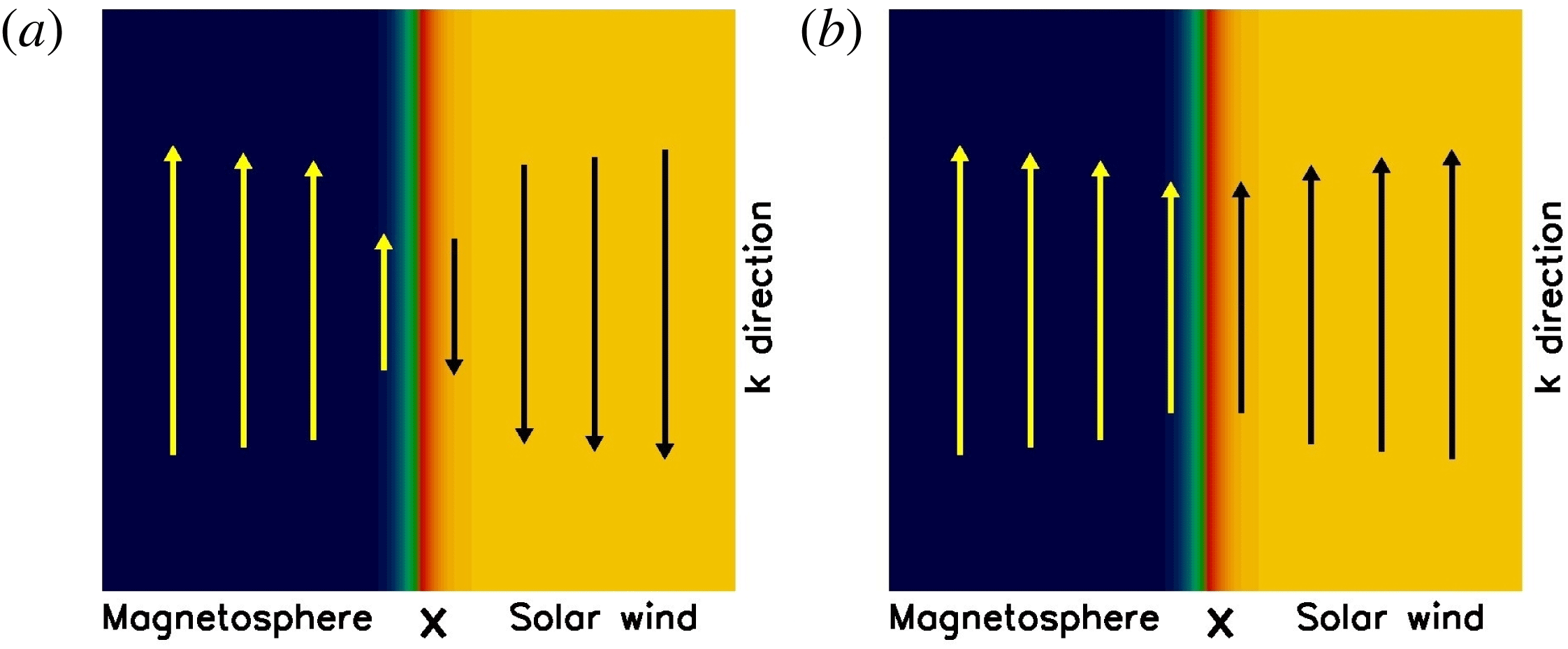
(a) Type I VIR configuration. Arrows represent the component of the equilibrium magnetic field lying in the dynamical plane defined by $\hat{\boldsymbol{x}}$ and $\boldsymbol{k}$ , which inverts its direction across the velocity shear layer the separates the two plasmas (blue and yellow regions) in relative motion. (b) Type II VIR configuration. The in-plane component is not necessary uniform but does not change its direction across the velocity shear layer.

This flute-like configuration has two important consequences: first of all, in a sheared magnetic field, the same place where the KHI grows can be a resonant surface for magnetic reconnection, leading to a possible coupling between the tearing instability (Furth Reference Furth1963; Coppi Reference Coppi1964; Wesson Reference Wesson1990) and the KHI (details are given in § 2.3). Furthermore, if we want to reduce the KH study to a 2-D problem, whose dynamical plane is defined by the inhomogeneity direction of the velocity shear, $x$ -axis, and by the wave vector of the most unstable mode (mainly aligned with the flow direction), we can expect to have two different configurations. In Type I VIR configuration (see figure 1) the in-plane component of the magnetic field $\hat{\boldsymbol{k}}\boldsymbol{\cdot }\boldsymbol{B}_{\text{eq}}$ becomes zero somewhere in the domain. For the sake of simplicity, in literature the null line is usually considered to be at the place where the maximum vorticity is. On the contrary, in Type II VIR configuration the in-plane component always differs from zero but, as in the first case, it is subdominant compared to the perpendicular one.

Figure 2.

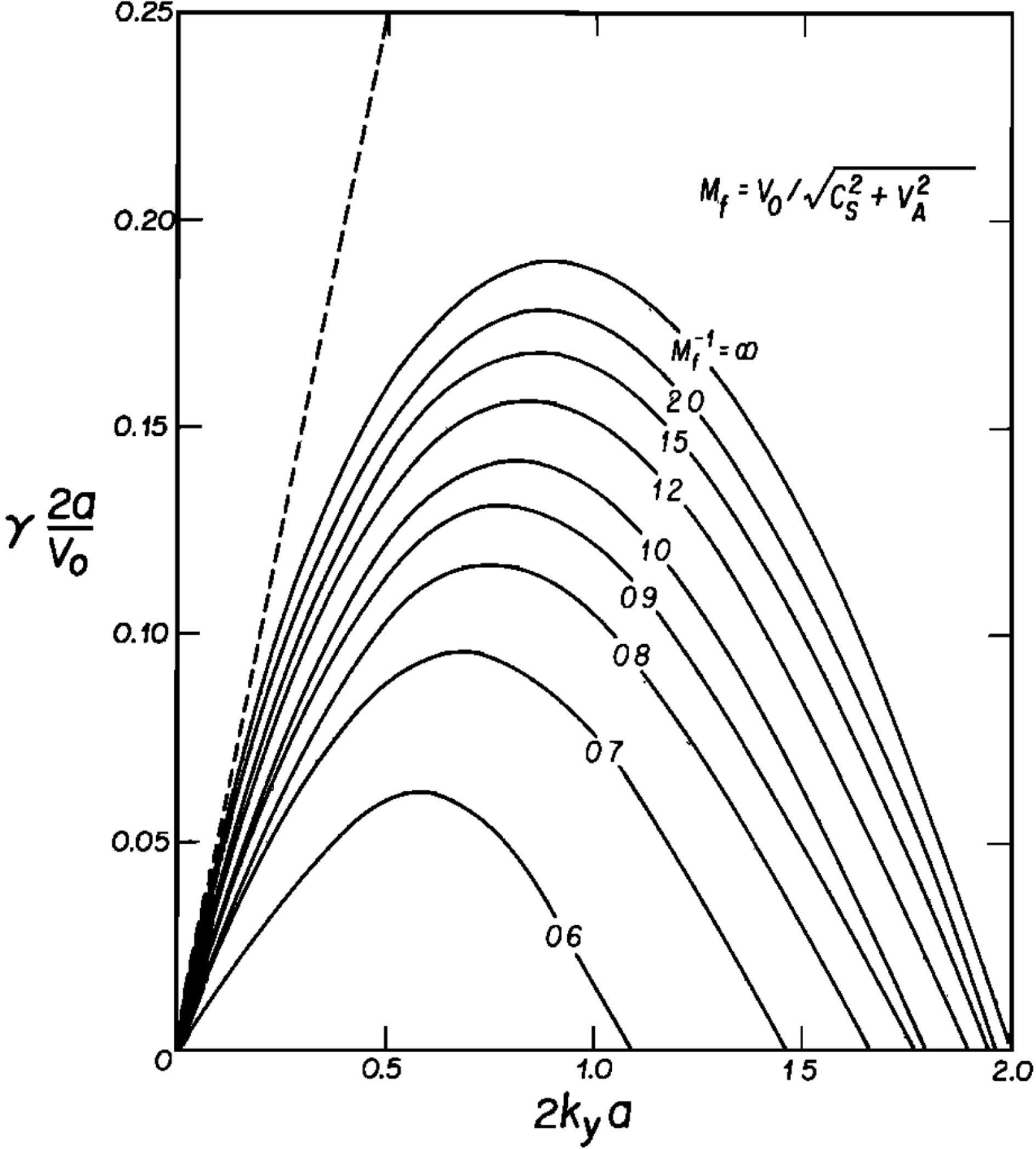
The normalized growth rate versus the normalized wave vector for the transverse case ( $\boldsymbol{B}_{\text{eq}}\bot \boldsymbol{U}_{\text{eq}}$ ).  $M_{f}$ is the magnetosonic Mach number defined by $V_{0}/(c_{s}^{2}+V_{A}^{2})^{1/2}$ , where $\boldsymbol{U}_{\text{eq}}=V_{0}/2\tanh (x/a)\hat{\boldsymbol{y}}$ , $c_{s}$ is the sound speed and $V_{A}$ the Alfvén velocity associated with the transverse magnetic field. The dashed line is the growth rate for the incompressible case with the discontinuous velocity profile.

On these grounds, Miura & Pritchett (Reference Miura and Pritchett1982) performed a parametric study of the stability of an hyperbolic tangent velocity profile in the presence of an uniform magnetic field, with different orientations as compared to the flow direction showing a complete stabilization of the mode for $M_{f}>2$ in the transverse configuration and for $M_{A,\Vert }<2$ when the fields are aligned. In the unstable cases he obtained the bell-shaped dispersion relation shown in figure 2. At the same time, in a vortex sheet configuration Pu et al. (Reference Pu1983) showed that for super-magnetosonic flow the KH growth rate drops but that the mode is still unstable. Furthermore the mode changes its nature from a surface wave, evanescent along the inhomogeneity $x$ -direction, to a radiating mode with an oscillatory behaviour still along the $x$ -direction. In some sense an important part of the free energy associated with the gradient of the equilibrium flow is converted into radiating magnetosonic waves, instead of feeding the instability. On the other hand the oscillatory mode is not confined to the shear region and penetrates deep inside the magnetosphere/magnetosheath regions. When the density difference between the two regions is taken into account, the pointing vector of the mode has a component toward the tenuous region, transferring energy to the magnetosphere. This behaviour has been confirmed adopting a more realistic continuous profile and radiating boundary conditions (Miura Reference Miura1990).

It is worth noticing that a density variation between the two streaming fluids decreases the growth rate and, more importantly, modifies the phase velocity of the mode. For a magnetospheric application, the phase velocity of linear waves or of the resulting vortices is directly related to the observed frequency of the measured fluctuations (in the usual case when the vortex evolution time is far greater than the transit time they take for passing a satellite). In an incompressible vortex sheet the phase velocity is given by the centre of mass velocity of the two fluids, nevertheless this value can change due to either a finite layer thickness and a non-uniform magnetic configuration (Walker Reference Walker1981) or to supersonic non-homogenous flow (Lai & Lyu Reference Lai and Lyu2006; Palermo et al. Reference Palermo2011a ) or even to finite Larmor radius (FLR) effects (Nagano Reference Nagano1979). In the first two cases the asymmetry of the velocity, magnetic or density profiles causes the mode to develop with a greater amplitude inside one of the two fluids. The precise shape of the mode is given by the ‘natural’ minimization of the stabilizing effects, due to magnetic tension or fluid compressibility, that are not equal inside the two fluids. As a consequence, the phase velocity of the mode is closer to the equilibrium velocity of the fluid which advects the largest part of the perturbations. In the last case FLR effects naturally introduce drift velocities, such as the ion diamagnetic one, that contribute to the advection of the perturbation and thus to the phase velocity of the mode.

2.2 Two-fluid and kinetic corrections to linear theory

When the shear layer thickness $a$ becomes of the order of the ion length scale (ion skin depth and/or ion gyroradius) ion inertia effects or FLR effects are expected to cause a departure from the linear MHD behaviour. These effects can still be described in a fluid framework considering the Hall term in the generalized Ohm’s law, for the former, and ion gyroviscosity in the motion equation, for the latter. In this context, Fujimoto & Terasawa (Reference Fujimoto and Terasawa1991) showed that, for $a=2d_{i}$ the Hall term introduces oscillations at the $d_{i}$ scale in the $x$ profile of the eigenfunctions. Nevertheless the values of the growth rate and of the real frequency are only slightly modified in this regime.

On the other hand, the growth rate and frequency of the wave mode can be significantly modified by FLR effects, as shown by the analytical solutions of an incompressible vortex sheet configuration. In particular, it has been shown that gyroviscosity can cause a complete stabilization of the mode at small wavelengths (Hans Reference Hans1968). Furthermore Nagano (Reference Nagano1978) has shown that such stabilization depends on the sign of $\unicode[STIX]{x1D734}_{\text{eq}}\boldsymbol{\cdot }\boldsymbol{B}_{\text{eq}}$ , the scalar product of the equilibrium vorticity and magnetic field: the mode is partially stabilized for $\unicode[STIX]{x1D734}_{\text{eq}}\boldsymbol{\cdot }\boldsymbol{B}_{\text{eq}}>0$ but, on the contrary, it is further destabilized for $\unicode[STIX]{x1D734}_{\text{eq}}\boldsymbol{\cdot }\boldsymbol{B}_{\text{eq}}<0$ . Adding a thermal pressure jump across the sheet, i.e. a diamagnetic drift velocity supported by this variation, stabilizes or destabilizes the large wavelength modes for positive or negative values of $\unicode[STIX]{x1D734}_{\text{eq}}\boldsymbol{\cdot }\boldsymbol{B}_{\text{eq}}$ , respectively, and completely stabilizes small wavelengths in both cases (Nagano Reference Nagano1979). Although the choice of a zero thickness vortex sheet can be questionable when FLR effects are retained, this simplified configuration can give important hints for the KH dynamics at the magnetopause. From a theoretical point of view, gyroviscosity must be calculated by expanding the full pressure tensor in power of the small parameter $\unicode[STIX]{x1D70C}_{i}/L$ , where $L$ is the characteristic spatial scale of plasma variations (see Cerri et al. (Reference Cerri2013) and references therein), so that this parameter cannot be taken as small in the vortex sheet limit. Nevertheless, vortex sheet models including FLR effects were able to suggest a possible explanation of the LLBL asymmetry observed at the Dawn and Dusk sides, having the opposite sign of $\unicode[STIX]{x1D734}_{\text{eq}}\boldsymbol{\cdot }\boldsymbol{B}_{\text{eq}}$ . This behaviour has been confirmed by numerical simulations considering a compressible plasma and a shear layer with $a\gg \unicode[STIX]{x1D70C}_{i}$ (Huba Reference Huba1996)Footnote ⁴ , for which the gyroviscous approximation is justified.

The vortex sheet configuration has been investigated using the drift kinetic equations, able to include wave–particle interaction effects. In this context the main result is that the thermal ions can resonate with the KH mode with a phase velocity of the order of the thermal velocity. This is the case at the Earth’s magnetopause where the sonic Mach number is of order one and the phase velocity is of the order of the flow velocity. The effect of this interaction is a reduction of the KH growth rate and of the energy flux associated with the KHI toward the magnetosphere. Indeed part of the free energy provided by the flow is employed in heating the background plasma, instead of feeding the instability (Pu Reference Pu1989).

2.3 Coupling with other modes

As suggested before the KHI could couple with other kinds of modes. In particular, when the conditions for magnetic reconnection to occur are satisfied somewhere inside the velocity shear layer, the tearing mode could be unstable at the same place of the KHI and the two instabilities may couple, even if the main driver remains the KHI. These conditions are given by, first of all, the presence of a sheared magnetic field as well as by the existence of at least one resonant surface defined by $\boldsymbol{k}\boldsymbol{\cdot }\boldsymbol{B}_{\text{eq}}=0$ . The simplest suitable configuration (monotonic $\boldsymbol{k}\boldsymbol{\cdot }\boldsymbol{U}_{\text{eq}}$ and $\boldsymbol{k}\boldsymbol{\cdot }\boldsymbol{B}_{\text{eq}}$ profiles) is the one adopted for investigating Type I VIR (see figure 1). In the context of a MHD description including a small resistivity or a finite electron mass, it has been shown that the KHI and the tearing mode are never unstable at the same time instant and thus do not couple at all. In fact, the tearing mode is strongly modified by the presence of the velocity shear layer but it is completely stabilized when the conditions for the KHI are fulfilled, i.e. when the magnetic tension associated with the sheared field is overwhelmed by the velocity driver (Hofmann Reference Hofmann1975; Einaudi & Rubini Reference Einaudi and Rubini1986; Chen & Morrison Reference Chen and Morrison1990; Faganello et al. Reference Faganello2010).

On the other hand, when the width of the magnetic and velocity shear layer is of the order of the ion skin depth, the Hall term changes the MHD dynamics and allows the tearing mode to be unstable above the KHI threshold (Chacón et al. Reference Chacón2003). The hybrid mode resulting from the coupling disappears well above the threshold, when the surviving pure KHI can develop vigorously. This is the usual regime that is investigated in the magnetospheric context, meaning that magnetic reconnection occurring in the Type I VIR configuration is not associated with a hybrid mode but it is simply forced by the KH velocity perturbations that pinch the current layer (see § 3.2 for details).

A different kind of coupling can occur between the KHI and Alfvén waves having a small component of their wave vector parallel to the magnetospheric magnetic field. This coupling is possible when the KHI changes its nature from a surface to a radiating one, i.e. around the threshold transition for super-magnetosonic KHI. Indeed, although its growth rate is far smaller, the super-magnetosonic mode can ‘explore’ deeper region inside the magnetosphere, where the magnitude of the magnetic field drastically increases. Indeed, at the location where the phase velocity matches the local Alfvén frequency, the mode can resonate with the magnetospheric lines. This possibility has been investigated by adopting a simplified slab geometry showing that this coupling can produce oscillations of the high-altitude magnetic field in the ultra low frequency (ULF) range (Fujita et al. Reference Fujita1996; Mann et al. Reference Mann1999; Mills & Wright Reference Mills and Wright1999).

2.4 Local stability analysis of the magnetopause

The first local stability analysis of the magnetospheric system has been performed by Sen (Reference Sen1965), applying the vortex sheet analysis to the ‘equilibrium’ fields of a model magnetopause. This study highlights the important role played by the magnetic shear between the IMF and the magnetospheric field for stabilizing the KHI and pointed out that the low-latitude region of the magnetopause is indeed unstable in the case that the shear between the IMF and the magnetospheric field is low enoughFootnote ⁵ .

More recently Farrugia et al. (Reference Farrugia1998) and Gratton et al. (Reference Gratton2003) applied the analytical results of both the vortex sheet and the continuous shear layer to a more refined model of the magnetopause. In this case the ‘equilibrium’ magnetic field advected by the solar wind is evaluated, at an imposed paraboloid boundary representing the magnetopause, using a global MHD code, once the upstream conditions are imposed, i.e. intensity and orientation of the IMF, as well as the unperturbed wind parameters. Looking at the stability of the layer, they showed that the tension associated with the (sheared) magnetic field dominates the velocity driver at high latitudes and completely stabilizes these regions, while the low-latitude regions remain unstable. At the same time, exploring different conditions for the IMF, they showed how local stability conditions change and how the unstable region migrates away from the equatorial region when the IMF deviates from a purely northward direction. In particular, it is shown that for a clock angle equal to $30^{\circ }$ , corresponding to a duskward component of the IMF equal to $1/3$ of the northward one, the unstable regions are in the northern and southern hemispheres at the Dawn and Dusk flanks, respectively. Indeed, these are the regions where the IMF and the magnetospheric field are parallel, and where KHI can grow by minimizing the magnetic tension.

3.1 Transverse configuration

The transverse configuration is characterized by a magnetic field strictly perpendicular to the flow direction corresponding to the simplest possible geometry describing the magnetized KH evolution. In this case the instability naturally develops with a wave vector $\boldsymbol{k}$ perfectly aligned with the velocity field $\boldsymbol{U}$ and perpendicular to the magnetic field. As a consequence, the 2-D plane of the dynamics is identified by the two perpendicular vectors $\hat{\boldsymbol{x}}$ and $\boldsymbol{k}$ , where $\hat{\boldsymbol{x}}$ is the direction of the shear assumed perpendicular to the flow direction.

Although extremely schematic, this configuration allows for a relatively deep study of the KHI where the field-aligned dynamics associated with Alfvén waves, whistler waves and magnetic reconnection is completely neglected. In the MHD framework only the fast magnetosonic waves survive for a strictly transverse configuration, leading to a nearly HD evolution of the system, once the sound speed is replaced by the fast magnetosonic velocity.

This system has been studied during the linear and nonlinear phase (Miura Reference Miura1982) by adopting a single-vortex configuration by taking a numerical box length $L_{y}$ along the flow direction equal to the FGM wavelength. In particular, when $M_{f}<2$ the usual KH surface mode can grow. The FGM grows and dominates, and eventually saturates in a single-vortex structure. As in the HD case, the vortex is characterized by a minimum of the total pressure inside the vortex and a maximum at the hyperbolic point of the velocity field, in between two consecutive vortices (note that a single-vortex configuration corresponds to a periodic chain of identical vortices). The saturated configuration, corresponding to a fully rolled-up vortex, can be seen as a nearly stationary equilibrium with a balance between the centrifugal force and the gradient of the total pressure. In this transverse configuration only the Reynolds stress contributes to the average stress, generated by the vortex, tangential to the unperturbed frontier. This effective eddy viscosity generates a momentum transfer between the two flowing plasmas and, as a consequence, a gradual broadening of the initial velocity profile, i.e. an effective viscous drag between the flowing solar wind and the magnetosphere. Anyway it is important to underline that the choice of $L_{y}=\unicode[STIX]{x1D706}_{\text{FGM}}=2\unicode[STIX]{x03C0}/k_{\text{FGM}}$ precludes the most important natural evolution of a nearly 2-D HD system, that is an inverse cascade process where close vortices merge generating larger and larger vortex structures (Winant & Browand Reference Winant and Browand1974).

Vortex pairing has been shown to be effective in 2-D magnetized simulations adopting an electrostatic kinetic description for the ions (Pritchett & Coroniti Reference Pritchett and Coroniti1984) or a classical MHD description of the shear layer (Wu Reference Wu1986) (see § 4.1 or hereafter). However, the first quantitative analysis of this process has been carried out by Miura (Reference Miura1997), adopting an MHD description with a periodic box along the flow direction $\hat{\boldsymbol{y}}$ and taking all the equilibrium quantities but the velocity as homogeneous. In this case, taking $L_{y}=4\,\unicode[STIX]{x1D706}_{\text{FGM}}$ , the process is described by the linear evolution, saturation and nonlinear coupling of the FGM, with mode number $m=m_{\text{FGM}}=4$ , and its subharmonics. 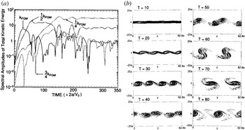Initially the FGM emerges but, after saturation, the $m=2$ amplitude becomes dominant (first vortex pairing) and finally the $m=1$ mode reaches the greatest amplitude (second vortex pairing). In figure 3 we show the long-time evolution of the mode driven by the interaction between couples of close vortices, namely vortex pairing, resulting in a progressive generation of larger and larger vorticesFootnote ⁶ . It is worth noticing that the effective viscosity associated with the Reynolds stress is far greater during each pairing process as compared to that observed during the linear evolution or early saturation of the FGM only. This means that vortex pairing can mediate the interaction between the flowing solar wind and the magnetosphere more efficiently than a chain of single saturated vortices. Indeed the broadening of the initial velocity profile is enhanced as pairing goes on. Using an even longer numerical box with $L_{y}=8\,\unicode[STIX]{x1D706}_{\text{FGM}}$ Miura (Reference Miura1999a ,Reference Miura b ) extrapolated the dominant wavelength as a function of time. Since the magnetopause vortices, while growing, move tailward at approximately one half of the solar wind speed and eventually merge, a linear relation between wavelength and time should correspond to an observed dominant wavelength growing with the distance from the subsolar point. Miura (Reference Miura1999b ) thus proposed an indirect method for inferring the velocity shear width near the subsolar point, by looking at the dominant KH wavelength at different locations along the magnetopause, an useful technique when vortex pairing is assumed to be effective (Foullon et al. Reference Foullon2008; Hasegawa et al. Reference Hasegawa2009; Lin et al. Reference Lin2014).

Figure 3.

(a) Temporal evolution of the amplitudes of the fundamental mode $m=4$ with $k=k_{\text{FGM}}$ (solid curve), the first subharmonic $m=2$ with $k=k_{\text{FGM}}/2$ (dot-dashed curve), the second subharmonic $m=1$ with $k=k_{\text{FGM}}/4$ (triple dot-dashed curve) and the Fourier mode $m=3$ with $k=3k_{\text{FGM}}/4$ (dotted curve) of the total kinetic energy integrated along $x$ , in a transverse configuration (Miura Reference Miura1997). (b) Contour lines of the $z$ component of the vorticity at eight different times (Miura Reference Miura1997). All amplitudes are normalized using $a$ , $V_{0}$ and the ion mass, where $\boldsymbol{U}_{\text{eq}}=V_{0}/2\tanh x/a\hat{\boldsymbol{y}}$ .

Relating the temporal evolution of a periodic vortex chain to the actual evolution of the KH modes propagating at the magnetopause is not trivial. Manuel & Samson (Reference Manuel and Samson1993) discussed the difference between the usual shear layer description, also known as ‘temporally developing’ shear layer and the ‘spatially developing’ shear layer. In the first case a periodic box is initiated with wave-like, non-localized perturbations, resulting in a layer that evolves in time but that, finally, is similar to itself all along the box. In the latter, inflow and outflow conditions for the flowing solar wind are imposed at the $y$ -boundaries (flow direction) of the numerical box and localized wavepackets are perturbed close to the inflow boundary. These packets evolve while moving along the flow direction, possibly giving rise to a perturbed layer that greatly varies along this direction since at the end the evolved wavepacket must get out from the simulation box. As discussed by Miura (Reference Miura1999b ), we can relate, via the phase velocity, what we observe in the periodic system, at a given time, to what would happen at a given spatial position in the corresponding ‘spatially developing’ layer. Nevertheless, one must bear in mind that no event is capable of affecting the prior development of the system. Therefore, adopting a ‘temporally developing’ layer, the dynamics occurring at a given magnetopause position (corresponding to a given time of the layer evolution) can influence the downstream dynamics only (corresponding to a later time of the layer evolution). On the contrary, in a ‘spatially developing’ layer a given event, at a given position, can influence the dynamics of the system also in the upstream region, compared to its position, and thus alter the development of the instability itself. Anyway, different HD and MHD ‘spatially developing’ simulations (Wu Reference Wu1986; Wei et al. 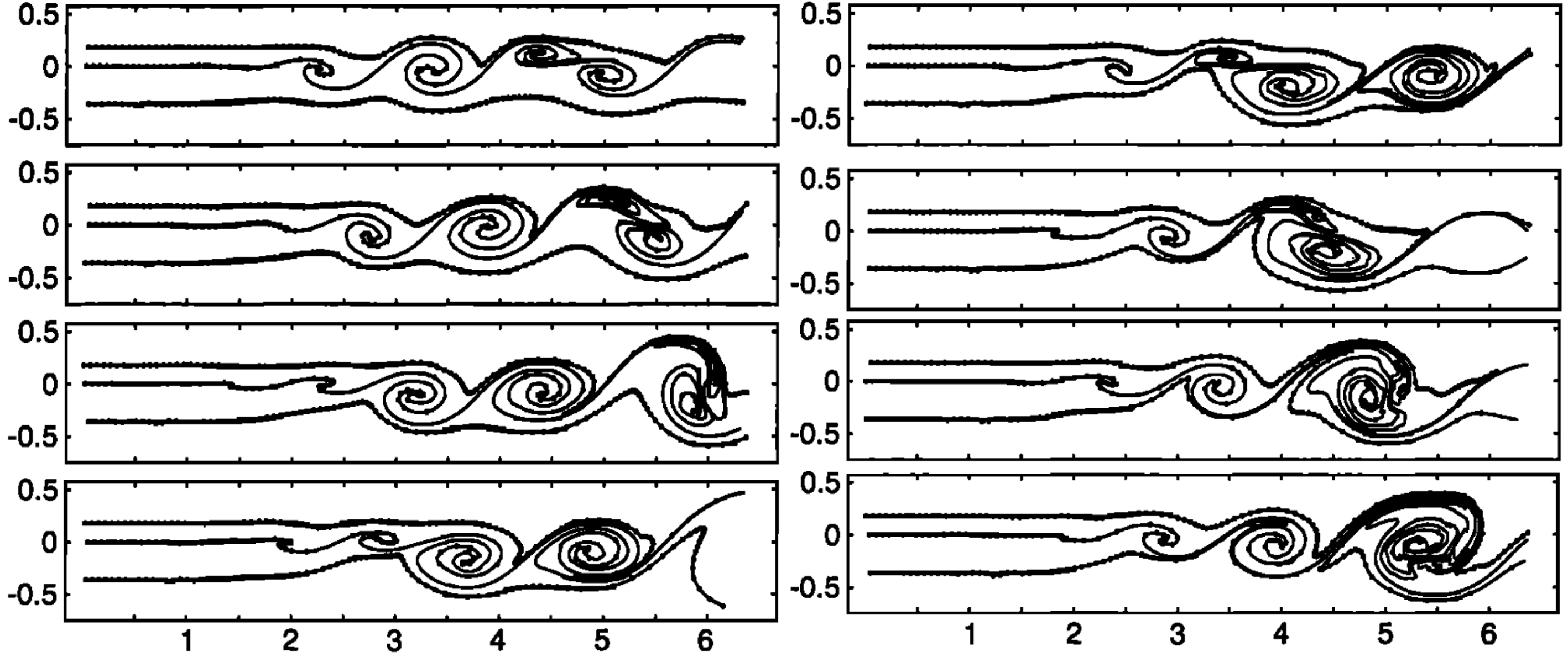Reference Wei1990; Manuel & Samson Reference Manuel and Samson1993; Wei & Lee Reference Wei and Lee1993), adopting a very long box as compared to $\unicode[STIX]{x1D706}_{\text{FGM}}$ and imposing the inflow at the upstream $y$ -boundary, show that the spatial evolution of the shear layer is similar to the one inferred from periodic simulations: localized perturbations grow moving along the flow giving rise to fully developed vortices that merge together eventually leading to a ‘nearly stationary’ perturbed layer where the average vortex length and amplitude grow linearly with distance from the initial perturbed location, as shown in figure 4. In a more rigorous way, Mills (Reference Mills2000) and Wright et al. (Reference Wright2000) demonstrated that the KHI changes its nature from ‘absolute’ to ‘convective’ instability depending on the adopted reference frame, the one moving at the group velocity of the mode or the Earth’s rest frame. In the first case, any point of a perturbed wavepacket grows in time and it is straightforward to define a temporal growth rate for a localized perturbation. In the second case, it does not because the localized perturbation moves away while growing. In this ‘convective’ case, it is more convenient to define a spatial growth rate by relating the distance covered by the wavepacket and its amplitude. In a similar way they defined the $e$ -folding distance, the spatial length a wavepacket takes to become nonlinear, showing that it is sufficiently short to allow the subsonic KHI to roll up at the dayside magnetopause and for the pairing process to be effective in the near tailFootnote ⁷ .

Figure 4.

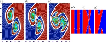
Snapshots of streamlines for a ‘spatially developing’ shear layer at different times (Manuel & Samson Reference Manuel and Samson1993). In each panel the top streamline is in the magnetosheath, the middle one at the centre of the shear layer and the bottom one in the magnetosphere. Note that the equilibrium flow is along the horizontal axis. Lengths are given in Earth’s radii.

Actually, the nonlinear evolution of the KHI can follow a totally different evolution, depending on the spatial non-uniformities of the initial equilibrium, in particular of the density field. Indeed once a single-vortex configuration has reached its saturation stage, the combined action of the spatial non-uniformities distorted by the folding motion and the vortical motion itself, can provide the favourable conditions for secondary instabilities to develop locally. On this point, when an equilibrium density variation across the shear layer is taken into account (as when passing from the magnetopause to the magnetosphere), it has been shown (Matsumoto & Hoshino Reference Matsumoto and Hoshino2004) that the primary KHI can drive secondary Rayleigh–Taylor and KH instabilities growing along the vortex arms. The former is related to the combined action of rotation, acting as en effective gravity $\boldsymbol{g}_{\text{eff}}$ , and density variations. In particular, depending on the relative orientation of $\boldsymbol{g}_{\text{eff}}$ and $\unicode[STIX]{x1D735}n$ , the folded boundary between the two plasmas alternating into the spiral arms of the vortices can be stable or unstable. The latter instead is related to the formation of velocity shear layers developing inside the vortex, due to the fact that, under the influence of the same centripetal force determined by the total pressure gradient, the denser plasma must rotate slower as compared to the tenuous one. These two instabilities can completely disrupt the vortex structure leading to the formation of a turbulent mixing layer, whose spectrum slope is determined by the initial density jump across the shear layer (Matsumoto & Hoshino Reference Matsumoto and Hoshino2004).

A different secondary instability that tends to reduce the vortex coherence was found by Nakamura et al. (Reference Nakamura2004) who showed that the in-plane current at the hyperbolic point can be unstable to a kink-like instability, once the electron inertia is included in the model. Per se this instability cannot disrupt the vortex but the perturbation generated can serve as a seed for secondary KHI. Depending on the sign of $\unicode[STIX]{x1D734}_{\text{eq}}\boldsymbol{\cdot }\boldsymbol{B}_{\text{eq}}$ the seed is quickly advected (as compared to the vortex evolution time) from the hyperbolic point to regions of the primary vortex that are unstable against secondary KHI or that are stable. This different behaviour suggests a possible Dawn/Dusk asymmetry resulting from the nonlinear evolution of KHI instability, with a vortex disruption far more pronounced at the Dusk side. A different reason for asymmetry can arise from the Hall term in the generalized Ohm’s law. In the quite extreme and unrealistic case when $a/d_{i}\ll 1$ (where $a$ represents both the width of the velocity and density shear layer), a new drift mode related to $\unicode[STIX]{x1D735}n\times \boldsymbol{B}$ could develop and influence the nonlinear evolution of a single vortex via the development of small-scale fluctuations (Huba Reference Huba1994). Depending on the relative direction of the phase velocity of the drift mode, proportional to $\unicode[STIX]{x1D735}n_{\text{eq}}\times \boldsymbol{B}_{\text{eq}}$ , and of the KH mode, the broadening of the velocity profile at the single-vortex saturation can be more or less pronounced when compared to the usual MHD evolution. At the magnetopause the sign of $(\unicode[STIX]{x1D735}n_{\text{eq}}\times \boldsymbol{B}_{\text{eq}})\boldsymbol{\cdot }v_{\text{ph,KH}}$ is exactly the same as $\unicode[STIX]{x1D734}_{\text{eq}}\boldsymbol{\cdot }\boldsymbol{B}_{\text{eq}}$ and corresponds to a Dusk or Dawn flank configuration.

Figure 5.

Density isocontour after the saturation of the $m=2$ FGM, in the case of moderate density jump (a, $n_{\text{sh}}-n_{\text{sph}}=0.6\,n_{\text{sh}}$ ) and of larger density jump (c, $n_{\text{sh}}-n_{\text{sph}}=0.8\,n_{\text{sh}}$ ), in a transverse configuration. (b,d) Represents a cut of the simulation domain at $x=45$ , after pairing (b) or disruption (d) have taken place. It corresponds to the temporal profile of density, measured by a stationary synthetic spacecraft surveying the moving structures. Lengths are normalized using the ion skin depth and density using the $n_{\text{sh}}$ (Faganello et al. Reference Faganello2008a ).

Adopting a ‘more realistic’ configuration (i.e. using a numerical box longer than $\unicode[STIX]{x1D706}_{\text{FGM}}$ ) secondary instabilities developing inside each vortex compete with the merging process. In this context it was clearly shown that the system evolution presents a bifurcation depending on the magnitude of the equilibrium density jump across the initial shear layer (Faganello et al. Reference Faganello2008a ). 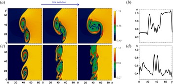In the case of a moderate density jump, the pairing process naturally proceeds. On the contrary, for a larger jump the secondary Rayleigh–Taylor instability takes over and the vortices are completely disrupted. As discussed before, this kind of schematic study (transverse configuration, neglecting the out-of-plane dynamics and adopting a one-dimensional equilibrium) does not pretend to quantitatively predict the KHI evolution at the magnetopause but to show and analyse the different processes at play in such a system that can be selected by the different physical parameters. This approach therefore intends to suggest possible different evolutions of the system, that are qualitatively different and would be characterized by totally different observational signatures (e.g. see figure 5 for the signatures that would emerge by a satellite crossing either merged or disrupted structures). Looking at satellite data, it should be possible to determine the evolution path of the system and the mechanisms that should be effective at the magnetopause. In particular, the density pattern of a merged vortex, as measured by a stationary satellite surveying the moving structure, is similar to that of a single-vortex configuration, but have a bigger wavelength compared to the one expected to emerge from a typical magnetopause profile. This pattern exhibits a typical step-like profile, corresponding to a sharp density variation at the hyperbolic point (see figure 5 b, at $y=24\unicode[STIX]{x03C0}\simeq 75$ ) and to nearly flat profiles corresponding to the magnetospheric and magnetosheath arms of the vortex, together with finer structures related to the internal region of the vortex. On the contrary disrupted vortices, eventually forming a mixing layer, would show only filamentary, turbulent-like structures without any given periodicity as shown in figure 5(d).

When the dynamics along the $z$ -direction is switched on, HD secondary instabilities develop in a similar way, having the tendency to develop with a wave vector perpendicular to the magnetic field, as in the 2-D purely transverse configuration. However, a new kind of secondary instability can emerge (Matsumoto & Seki Reference Matsumoto and Seki2007), acting on the shoulder of a saturated single vortex seen as a rotating and axisymmetric equilibrium configuration. This instability can be seen as a generalization of the magnetorotational instability (Velikhov Reference Velikhov1959; Chandrasekhar Reference Chandrasekhar1961; Balbus & Hawley Reference Balbus and Hawley1991, Reference Balbus and Hawley1998), having a finite $k_{z}$ but also a finite azimuthal mode number. Nevertheless for $\unicode[STIX]{x1D6FD}=8\unicode[STIX]{x03C0}P_{\text{eq}}/|\boldsymbol{B}_{\text{eq}}|^{2}$ of the order of the unity, as is the case at the Earth’s magnetopause, the vertical wavelength $\unicode[STIX]{x1D706}_{z}$ of this secondary instability is of the same order as the connection length between KH stable (high-latitude) and unstable (low-latitude) regions. This fact suggests that equilibrium variations along the $z$ -direction and line tying should be taken into account. In this case the plasma and magnetic dynamics seem to be dominated by totally different phenomena as compared to magnetorotational instability (see § 5 and Faganello et al. (Reference Faganello2012b ) for further details). The importance of the line-tying effect, completely missed in a 2-D geometry, can be easily understood by noticing that the Earth’s field lines and the solar wind field lines, both connected and anchored in the vortices developing in the equatorial region, are stuck at the Earth or free to move, respectively.

3.2 Type I VIR configuration

The equilibrium configuration leading to a Type I VIR is shown in figure 1(a). The in-plane component of the equilibrium magnetic field inverts its direction across the velocity shear layer. As discussed before this configuration corresponds to a 2-D projection of the full three-dimensional system having a sheared magnetic field on the 2-D plane defined by $\hat{\boldsymbol{x}}$ and $\boldsymbol{k}$ . Indeed, at least in the idealized case where the equilibrium does not vary along the $z$ -coordinate, the FGM has a wave vector that is not perfectly aligned with the flow direction $\hat{\boldsymbol{y}}$ but naturally orients itself such that $\boldsymbol{k}_{_{\text{FGM}}}\boldsymbol{\cdot }\boldsymbol{B}_{\text{eq}}\simeq 0$ , in order to limit as much as possible the impact of magnetic tension. For the sake of simplicity, in the literature the null line of the in-plane magnetic field is usually located where the maximum vorticity is, assuming that the system is fairly symmetric with respect to the shear layer (Southwood Reference Southwood1968; Contin et al. Reference Contin2003). This configuration allows us to explore the linear and nonlinear behaviour of magnetic reconnection, possibly occurring at the resonant surface where the in-plane magnetic field goes to zero, in the regime where the KHI grows vigorously. From the magnetospheric point of view it corresponds to a configuration where the IMF is not perfectly aligned with the Earth’s dipole and $\boldsymbol{k}$ takes a finite $z$ -component for minimizing the magnetic tension effect exactly at the magnetopause, at low latitude.

The first numerical studies on Type I VIR where performed in the resistive reduced-MHD framework and, although barely resolved, clearly showed that reconnection at the null line is forced by the velocity field generated by the growing KHI (Liu & Hu Reference Liu and Hu1988; Fu et al. Reference Fu1995a ,Reference Fu b ). 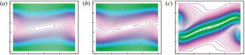Indeed when the in-plane Alfvénic Mach number $M_{A,\Vert }$ , defined using the asymptotic value of the in-plane Alfvén velocity $V_{A,\Vert }$ , is greater than a critical value (let say order one), the velocity driver wins over magnetic stabilization and the KHI can grow, nearly independently from a small value of the resistivity. In this case the velocity field around the KH hyperbolic point has the same structure of the usual inflow/outflow pattern that characterizes a reconnection X-point but, this time, imposed by the growing ideal instability. The result is that field lines belonging at the two different regions are pushed together at the hyperbolic point where a small but finite resistivity acts to break the frozen-in condition and eventually allows for reconnection, as shown in figure 6. This process is characterized by a reconnection growth rate comparable to that of the KHI (far greater than that expected for spontaneous reconnection) and by the formation of a magnetic island that coincide with the vortex structure (X-point at the hyperbolic point and O-point in the vortex core).

Figure 6.

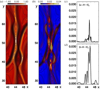
Snapshots of streamlines (a), magnetic field lines of the in-plane magnetic field (b) and isocontours of the $z$ -component of the current density (c), for resistive Type I VIR in a single-vortex configuration (Knoll & Chacón Reference Knoll and Chacón2002). The hyperbolic point, where the current is pinched and reconnection occurs, is in the centre of the numerical box. Note that in this case the equilibrium flow is along the horizontal axis. Lengths are in arbitrary units.

More recent, better resolved MHD simulations (Chen et al. Reference Chen1997; Knoll & Chacón Reference Knoll and Chacón2002) have confirmed that, when $M_{A,\Vert }>2$ , the KHI starts to grow and the reconnection rate is the same as the ideal instability. Indeed it scales with $\unicode[STIX]{x0394}U$ and has a very weak dependence with respect to $\unicode[STIX]{x1D702}$ . Furthermore these studies relate the reconnection at hyperbolic point to the pinching of the pre-existing equilibrium current layer, leading to a local and enhanced resistive dissipation. In particular Knoll & Chacón (Reference Knoll and Chacón2002) discussed how the width of the original current layer drops during the early evolution of the KHI down to a value $\unicode[STIX]{x1D6FF}\sim S^{-1/2}$ such that the dissipation rate of magnetic flux, nearly equal to $1/(\unicode[STIX]{x1D6FF}^{2}S)$ , equates the growth rate $\unicode[STIX]{x1D6FE}_{_{\text{KH}}}$ imposed by the ideal instability. Here $S=(\unicode[STIX]{x1D702}/aV_{_{A,\Vert }})$ is the Lundquist number and $a$ is the half-width of the equilibrium vortex/current layer.

It is worth to stress that in the case of an initial uniform in-plane magnetic field, reconnection can occur only during the nonlinear phase of the KHI, when the vortices are fully rolled up, and only for sufficiently large $M_{A,\Vert }$ (see § 3.3 for details). Indeed, the rolling up of the magnetic lines, advected by the vortex motions generated by the KHI, is able to build-up local inversion layers where reconnection can occur. On the contrary, as already stated, a Type I VIR starts acting during the early phase in the initial, pinched current layer and does not necessitate of rolled-up vortices to develop. This fact has been confirmed adopting a collisionless fluid description where reconnection is allowed by finite electron inertia. Nakamura & Fujimoto (Reference Nakamura and Fujimoto2006) showed that a collisionless Type I VIR occurs at $2<M_{A,\Vert }<5$ , when the magnetic tension is high enough to inhibit the vortex rolling up, as well at $M_{A,\Vert }>5$ when rolling up takes place. Also in the collisionless description, the reconnection evolution (and so the growth rate) is completely overcome by the evolution of the KHI and it is independent from the value of the electron to ion mass ratio (Nakamura & Fujimoto Reference Nakamura and Fujimoto2006; Nakamura et al. Reference Nakamura2006).

Figure 7.

Snapshots at different times of collisionless Type I VIR in a multiple vortices configuration (Nakamura & Fujimoto Reference Nakamura and Fujimoto2008). Field lines are drawn in black, colours represent the pressure variations compared to the equilibrium value. In smaller frames white arrows describe the fluid velocity field and crosses specify the locations of X-points. Note that in this case the equilibrium flow is along the horizontal axis. The half-width of the equilibrium vortex/current layer is $D=2d_{i}$ and the box length is $=8\unicode[STIX]{x1D706}_{\text{FGM}}=8\unicode[STIX]{x1D706}_{\text{KH}}=120D$ .

When a long numerical domain is adopted, it has been shown that the pairing process between different vortices still dominates the dynamics, both for high or low magnetic tension (Pu & Fu Reference Pu and Fu1997; Nakamura & Fujimoto Reference Nakamura and Fujimoto2008; Califano et al. Reference Califano2009). The magnetic islands, associated with different vortices, follow the same evolution and merge together, forming larger and larger islands corresponding to the new merged vortices. This evolution is shown in figure 7 (shaded coloured isocontours represent a pressure variation with respect to the equilibrium) starting from eight vortices associated with the $m=8$ FGM mode. Note that in the figures a single vortex corresponds to one blue structure while the yellow one represents the region in between. In particular, these structures are characterized by pressure minima inside each vortex (in blue) and pressure maxima in between (in yellow) corresponding to the hyperbolic points. During the evolution, the vortices progressively coalesce and their number decreases from eight to one (last frame). Magnetic islands follow the same evolution and coincide with the vortex structures in all frames.

A Type I VIR has important consequences on the transport properties of the system being able to create field lines connecting the two different plasmas, initially magnetically disconnected, on the left and right side of the original current/vortex layer. In this way a flux of mass across the original frontier can be established via parallel streaming of electrons/ions. We can thus infer that a mixing layer would develop inside the region occupied by vortices, and that its width grows as the vortex merging goes on. To quantify the impact of this streaming on the transport properties of the magnetopause and on the further dynamics of the vortices themselves, is not possible when adopting a fluid approach and, more than that, a 2-D geometry. This point will be discussed in the framework of a kinetic description in § 4.2. On the contrary, fluid simulations can describe the impact of magnetic reconnection on the transfer between kinetic and magnetic energy and their relaxation. In fact reconnection, locally breaking the frozen-in condition, allows the system to reach states of lower magnetic energy where the two different plasmas are no longer magnetically disconnected. These states would be forbidden by the topological constraint on the magnetic field in the case of an ideal evolution. In a single-vortex configuration, Keppens et al. (Reference Keppens1999) showed that the magnetic energy, enhanced by the KHI via the bending and compression of field lines, grows slower and saturates at a lower level when the equilibrium in-plane magnetic field is inverted, compared to a situation where it is initially unidirectional (and uniform). Indeed in the former case a Type I VIR acts even before the formation of vortices and releases the tension of bent field lines, while in the latter case reconnection can occur only in the late nonlinear phase after the rolling up of magnetic lines caused by the vortex motion has built-up local inversion layers (see § 3.3 for details).

3.3 Type II VIR configuration

In figure 1(b), we show the configuration leading to Type II VIR. In this case, the equilibrium magnetic field component parallel to the wave vector does not change sign across the vortex layer. The first nonlinear study of this configuration (Miura Reference Miura1982) neglected the out-of-plane component of the magnetic field. In this case, at least for the linear and early nonlinear phases, the behaviour of the KHI is controlled by $M_{A,\Vert }$ for the stabilization related to the magnetic tension, and by $M_{s}$ for the stabilization related to plasma compressibility (Miura Reference Miura1982). When an important out-of-plane component of the magnetic field is added, as it is in general the case at the magnetopause, $M_{f}$ determines the compressibility of the system. Miura (Reference Miura1982) focussed his attention on the role of the magnetic tension on the KH dynamics, neglecting all possible effects related to density or temperature variation in the equilibrium configuration. In a subsonic MHD regime, he showed that the degree of rolling up of the vortices is determined by $M_{A,\Vert }$ . The higher $M_{A,\Vert }$ , the easier it is to fold field lines, the more rolled up the vortices are. The same is true for the energy transfer from the mean flow to the magnetic part: the higher $M_{A,\Vert }$ , the more efficient the transfer is. Furthermore, Miura (Reference Miura1982) showed that the effective viscosity associated with the KH vortices is dominated by the Maxwell stress, contrary to the transverse case where it is dominated by the Reynolds stress (see § 3.1). In both cases the resulting momentum transfer across the frontier is large enough to explain the convection observed in the inner magnetosphere (Axford & Hines Reference Axford and Hines1961).

Figure 8.

The nonlinear configuration created by KHI, allowing for reconnection to occur along the inversion layers located at each vortex arm (Tenerani et al. Reference Tenerani2011). Field lines are drawn in black. Colours represent the plasma density, going from 0.7 (blue) to 1 (red), in arbitrary units. Lengths are normalized using the value of the ion skin depth on the right of the numerical box. The chosen half-width of the equilibrium velocity shear layer is $3\,d_{i}$ , resulting in a FGM wavelength $\unicode[STIX]{x1D706}_{\text{FGM}}\simeq 45\,d_{i}$

In a 2-D description the existence of an inversion layer for the in-plane magnetic field is a necessary condition for reconnection. Even starting from an uniform magnetic field, such a layer can be generated by the KH dynamics rolling up the magnetic field lines, as shown by Frank et al. (Reference Frank1996) and Min & Lee (Reference Min and Lee1996). This configuration is illustrated in figure 8 where field lines escaping from the two different left and right plasmas (typically the magnetospheric and the solar wind ones) are advected into the vortices and folded along each blue or red arm. By looking at the black isolines representing the in-plane flux function, we see that even if the vortex rolls up the two different plasmas, the left and right lines remain well connected to the left and right plasmas, respectively. Therefore, a rolled-up vortex is not an efficient structure for mixing except for the fact that the classical diffusion between adjacent arms is enhanced because of the strongest gradients with respect to the initial large-scale shear (but still not sufficiently efficient to explain the observed mixing). Nevertheless this configuration is favourable for reconnection to occur, in particular at the magnetic inversion layers created along the vortex arms.

Contrary to Type I, this kind of VIR occurs as a secondary instability during the nonlinear phase of the KHI, once the favourable conditions have been created by the fully rolled-up vortices. Type II VIR can therefore compete with the HD evolution of the vortices and lead to their partial disruption. In the unrealistic limit of a single-vortex configuration, it has been shown (Frank et al. Reference Frank1996; Jones et al. Reference Jones1997; Keppens et al. Reference Keppens1999) that reconnection eventually disrupts the full vortex structure and that the system relaxes toward a laminar flow with $\boldsymbol{B}$ and $\boldsymbol{U}$ aligned. During the early nonlinear phase there is a net energy transfer from the kinetic to the magnetic energy, due to the rolling up of field lines. As soon as reconnection occurs and relaxes the tension state of the system, the magnetic energy decreases but remains greater than its initial level due to the presence of persisting flux ropes (magnetic islands) generated by reconnection.

We consider now the impact of the intensity of the in-plane magnetic field on the development of the KHI and of Type II VIR. In a single-vortex configuration, Jones et al. (Reference Jones1997) identify three different regimes: ‘strong field’, ‘weak field’ and ‘very weak field’ regime. In the first case, $M_{A,\Vert }<5$ , the KHI is nonlinearly stable and remains wave-like also during the saturation phase, so that Type II VIR cannot occur. In the second one, $5<M_{A,\Vert }<20$ , the magnetic tension cannot prevent the formation of rolled-up vortices, reconnection occurs as a secondary instability and finally completely disrupts the vortex structure. On the contrary, in the ‘very weak field’ regime, $20<M_{A,\Vert }<50$ , reconnection still occurs but it is unable to influence the nearly HD evolution of the vortex. It simply enhances the level of dissipation of the system eventually leading to a saturation of the vortex.

With the aim of comparing simulations and observations, Otto & Fairfield (Reference Otto and Fairfield2000) performed 2-D single-vortex simulations starting from an equilibrium configuration taken from observations. They showed that a Type II VIR is efficient, mainly along the dense, magnetosheath arms of the vortex. Flux ropes, corresponding to ‘blobs’ of magnetosheath plasma, are detached from the vortex arms and enter the magnetospheric region. Assuming that this process corresponds to a mass entry into the magnetosphere and looking at the mean entry velocity of these blobs, Nykyri & Otto (Reference Nykyri and Otto2001, Reference Nykyri and Otto2004) argued that the inferred entry rate is compatible with the one expected during northward periods (Borovsky et al. Reference Borovsky1998).

Vortex disruption and blob production in the ‘weak field’ regime have been confirmed by two-fluid simulations of single-vortex configuration (Nakamura & Fujimoto Reference Nakamura and Fujimoto2005, Reference Nakamura and Fujimoto2006) showing that Type II reconnection occurs only along the ‘same’ field lines (magnetosheath or magnetospheric ones, folded along the vortex arms). However in this way the reconnected lines do not connect plasmas of different origin and do not allow for a true mixing. At the same time the magnetosheath blobs that are injected into the magnetosphere maintain their coherence (as plasma/magnetic structures) also during the late nonlinear phase and eventually come back to their original side due to the tension of magnetospheric lines. In this way Type II VIR cannot account for mass entry into the magnetosphere. One concludes that the whole process seems to be quite robust and independent of the fluid plasma description adopted (from resistive MHD to a two-fluid description, including or not the electron mass). This fact can be surprising but actually, given the single-vortex configuration, it is not since the early dynamics is large scale (let say MHD) as compared to $d_{i}$ . Including the Hall term leads to a small increase of the KH growth rate (Nykyri & Otto Reference Nykyri and Otto2004) and the fact that the magnetic field is now frozen in the electron motion just decreases the importance of magnetic tension but does not alter the large-scale dynamics. Nevertheless, once thin current layers have been created, Hall and two-fluid physics could, and so do, influence the local dynamics of reconnection acting as a secondary instability on a different time scale with respect to MHD. However, reconnection proceed on a magnetic configuration that is quite stationary, that of the saturated single vortex. A faster or slower reconnection rate could simply change the characteristic time when blobs are detached and the vortex is disrupted, but not the final global evolution of the system.

This picture strongly changes (see § 3.1) if merging between vortices is allowed. This is even more important in the Type II VIR configuration where actually the dominant process is the vortex pairing and almost never vortex disruption, as shown by Baty et al. (Reference Baty2003), for all possible values of the in-plane magnetic field (we will discuss the role of density variations in § 3.3.1). In addition, it has been shown (Faganello et al. Reference Faganello2008b , Reference Faganello2009) that reconnection occurs during the merging between close vortices. It is actually driven by the pairing process instead of being driven by the vortical motion of each single vortexFootnote ⁸ .

Figure 9.

(a–c) Plasma passive tracer and magnetic field lines in the $(x,y)$ -plane at three different times during the pairing process ( $t=426,440,480$ ) in a Type II VIR configuration (Faganello et al. Reference Faganello2008c ). In the equilibrium configuration density and temperature profiles are constant, $M_{A,\Vert }=20,~M_{A,\bot }=1,~M_{s}=1$ . Lengths are normalized using $d_{i}$ , time using the ion cyclotron frequency. The chosen half-width of the equilibrium velocity shear layer is $3\,d_{i}$ , resulting in a FGM wavelength $\unicode[STIX]{x1D706}_{\text{FGM}}\simeq 45\,d_{i}$ . (d–f) Schematic representation of the magnetic field lines topology in the region between the two pairing vortices. The lines shown represent the local features of the field line ribbon: the two inversion layers at $t=426$ , reconnection acting at $t=440$ and the final new magnetic topology.

Figure 10.

A zoom-in on the region between the two pairing vortices of figure 9, at $t=440$ . (a) Shaded isocontours of the perpendicular current density and magnetic field lines. (b) Ion decoupling region ( $\boldsymbol{u}_{i}\times \boldsymbol{B}+\boldsymbol{E}\neq 0$ ) and magnetic field lines. (c,d) Electron (c) and ion (d) decoupling region along the $x$ -direction at $y=47$ . Quantities are normalized using $d_{i}$ , the ion mass and cyclotron frequency. It is evident the scale separation between the ion and the electron decoupling region, leading to ‘fast’ magnetic reconnection.

In figure 9(a–c) we show the magnetic field lines and a plasma passive tracer marking the dynamics of a Type II VIR event, in the case of constant equilibrium density. The magnetosheath and magnetospheric plasmas are represented by the red and blue colours, respectively. A distinct feature of the ‘weak field’ regime is the creation of a ‘ribbon’ of compressed field lines that separates the magnetosphere (blue) and magnetopause (red) plasmas, thus representing a magnetic frontier in such a simplified 2-D description. The ribbon is rolled up more and more by the vortical motion and folded twice during the pairing process, corresponding to the creation of two magnetic inversion layers located in between the vortices. Magnetic reconnection acts first in these two layers, erodes the ribbon and changes the global topology of the full system, leading to the creation of a new, magnetic frontier. This frontier still separates the main part of the original blue and red regions, but large-scale blobs (the entire core of each vortex) have been injected in the opposite regions. In figure 9(d–f), we give a sketch of this process.

Plasma injection goes on at each pairing process without a significant return of blobs to their original region. The necessary condition for blob injection is given by the folding of the magnetic ribbon during the merging and not simply by the rolling up of the vortices. For $M_{A,\Vert }=5$ the last condition is fulfilled but not the first, and injection is not observed, even if pairing between vortices still proceeds. For $M_{A,\Vert }=10$ or larger both conditions are satisfied and injection occurs (Faganello et al. Reference Faganello2009).

Contrary to the single-vortex configuration, when pairing is allowed, the evolution of the magnetic topology, and thus blob injection, is not independent from the adopted plasma model since the magnetic configuration, on which reconnection occurs, evolves in time: vortices move while merging and are not simply nearly stationary, saturated structures. Reconnection must be rapid enough to take advantage of the favourable conditions that are created by the large-scale motions, and that can be rapidly modified by the system itself. On this point Faganello et al. (Reference Faganello2008b ,Reference Faganello c ) have shown that the typical width of the current layers, in between the merging vortices, is of the order of $d_{i}$ . In these region reconnection is Hall-dominated and proceed on a time scale not too far from the local Alfvén timeFootnote ⁹ . In this case reconnection is rapid enough to cut the magnetic ribbon thus changing the global topology. On the contrary, if the plasma description is oversimplified, as it is for resistive-MHD, reconnection still occurs in the same current layers but on a time scale too slow to change the global topology before these current layers are modified by the large-scale motion. In conclusion, the final magnetic topology, and so plasma transport across the original frontier, strongly depends on the correct ‘minimal’ choice for describing the plasma evolution and, in particular, reconnection. In the usual magnetospheric case, where plasma compressibility can easily create sub- $d_{i}$ current layers, the ‘minimal’ ingredient required beyond MHD is the Hall term.

The cases discussed before underline the importance of choosing the correct plasma model to describe the dynamics of a multi-scale problem such as the interplay between large-scale KHI and magnetic reconnection. Furthermore, blob injection and the consequent solar wind entry into the magnetosphere has been described here in a simplified 2-D geometry where all quantities are invariant along the $z$ -direction. In some sense we cannot determine the magnetic connectivity of the flux rope that corresponds to each plasma blob and thus we cannot state that it has been incorporated into the magnetosphere, in other words that it is connected to the Earth at both poles.

3.4 Super-magnetosonic flows

As a matter of fact, the KHI is effective also when $M_{f}$ is larger than one. Two peculiarities distinguish this regime with respect to the sub-magnetosonic one. First of all the mode is no longer localized at the interface as it becomes oscillatory instead of evanescent, along the $x$ -direction. Second, the vortices act as obstacles in a super-magnetosonic flow and thus generate shocks in the magnetospheric or magnetosheath regions, depending on the large-scale fields’ configuration. The first point can impact the energy transport from the solar wind to the magnetosphere, as an oscillatory mode can penetrate deeper inside the magnetosphere. The shock formation can impact the development of the KHI itself and that of secondary instabilities growing on the shoulder of primary vortices.

Concerning the first point, Miura (Reference Miura1990) showed that the nature of the KH mode is related to the convective Mach number in the magnetosheath/magnetosphere, defined as $M_{c,\text{sh/sph}}=|U_{\text{sh/sph}}-v_{\text{ph,KH}}|/c_{f,\text{sh/sph}}$ , where $U_{\text{sh/sph}}$ and $c_{f,\text{sh/sph}}$ are the flow velocity and the phase velocity of the fast magnetosonic mode along the $\boldsymbol{k}$ -direction in the magnetosheath or in the magnetosphere respectively. Indeed the mode turns out to be super-magnetosonic in one of the two region if the corresponding convective Mach number is greater than oneFootnote ¹⁰ . The penetration length of the mode into each domain is $\ell =\unicode[STIX]{x1D706}_{\text{KH}}/2\unicode[STIX]{x03C0}(1-M_{c,\text{sh/sph}}^{2})^{1/2}$ . For the magnetic configuration chosen in Miura (Reference Miura1990, Reference Miura1992), the mode penetrates into the magnetosphere and its pointing flux carries energy from the magnetosheath toward the Earth. On the other hand, even if the KH perturbation reaches more interior regions, its amplitude is strongly decreased in the super-magnetosonic regime and the energy supply finally decreases, as compared to the sub-magnetosonic regime. The same is true for the momentum transport, as the effective eddy viscosity decreases (Miura Reference Miura1992), suggesting that momentum and energy transport related to the KHI are more efficient in the dayside region of the magnetopause where the convective Mach number is usually smaller than one. After the terminator plane (day–night boundary) the draping of magnetic field lines around the magnetopause starts to accelerate the magnetosheath flow, finally leading to super-magnetosonic conditions in the far tail (Spreiter et al. Reference Spreiter1966).

The definition of a convective Mach number, including the phase velocity of the mode, allows one to consider KH vortices as obstacles with respect to the plasma flow streaming in each of the two regions. In fact, as soon as the convective Mach number is bigger than one, a series of shocks is generated by the interaction between each KH vortex and the flow (Miura Reference Miura1992). Depending on the KH phase velocity and the plasma parameters in each region, the shocks extend deep into the magnetosheath or into the magnetosphere (Miura Reference Miura1984, Reference Miura1992; Palermo et al. Reference Palermo2011a ). In 2-D simulation assuming $\boldsymbol{k}$ parallel to the flow, quasi-perpendicular shocks develop inside the magnetosphere, where the magnetic field is nearly perpendicular to the dynamical plane. In the magnetosheath region shocks can be quasi-perpendicular or quasi-parallel, depending on the relative orientation of the IMF and the flow (Miura Reference Miura1992; Lai & Lyu Reference Lai and Lyu2006; Palermo et al. Reference Palermo2011a ).

The interaction between the structures of the shocks and the vortices can affect the KHI saturation and its late nonlinear evolution. First of all the saturated size of the vortices is determined by the convective Mach number. On one hand the flow velocity suddenly decreases across each shock and becomes sub-magnetosonic, allowing for the growth and rolling up of the vortices. For an increasing Mach number, the shock angle gets steeper and the sub-sonic area behind it gets smaller, inducing a reduction of the vortex size. On the other hand the pressure variations that develop in a faster flow are bigger and tend to push the vortex to grow. The final size of the saturated vortices is thus determined by a balance between these two opposite effects (Kobayashi et al. Reference Kobayashi2008).

Concerning the late evolution, the sharp variations associated with the shock can trigger the development of secondary instabilities at the boundary region of a vortex, as observed in Palermo et al. (Reference Palermo2011b ) and Henri et al. (Reference Henri2012).

4.1 Transverse configuration

In spite of the fact that the transverse configuration is the simplest possible one, it shows up the difficulty of a kinetic treatment of plasmas in systems that are not homogeneous. Even the initial equilibrium configuration describing the shear layer is a source of problems since the shifted Maxwellian usually adopted to describe the sheared mean velocity of a population of particles at a given temperature and density is far from being a kinetic equilibrium. Simply imposing a balance between the thermal pressure and the magnetic one (or even taking uniform pressure, density and magnetic field), as in the case of a one-dimensional fluid equilibrium, does not guarantee the stationarity of the configuration leading to a quick relaxation of the initial configuration over a few cyclotron periods $\unicode[STIX]{x1D6FA}_{i}^{-1}$ , a time scale far shorter as compared to the KH one (Pritchett & Coroniti Reference Pritchett and Coroniti1984; Nakamura et al. Reference Nakamura2010; Cerri et al. Reference Cerri2013). The smaller the ratio $a/\unicode[STIX]{x1D70C}_{i}$ , the more important the relaxation. However the modification of the initial velocity profile is not dramatic in the presence of a guide field, as typically observed in the magnetospheric case. Starting from a typical shear layer (e.g. a hyperbolic tangent profile for the mean velocity $U(x)\hat{\boldsymbol{y}}$ ) the relaxed one still has a similar shape and asymptotic values for all plasma quantities. The new profile is unstable against KHI and thus suitable for looking at its linear and nonlinear development.

In the case of $\unicode[STIX]{x1D734}\boldsymbol{\cdot }\boldsymbol{B}>0$ the modifications of the initial shear layer are minimal, while for $\unicode[STIX]{x1D734}\boldsymbol{\cdot }\boldsymbol{B}<0$ Nakamura et al. (Reference Nakamura2010) and Henri et al. (Reference Henri2013) have shown that an important broadening of the layer can be generated by the self-reorganization of the system. This fact impacts the study of the kinetic KHI as from fluid theory we know that the nearly MHD dynamics of large-scale vortices strongly depends on the layer half-width $a$ . According to MHD theory the linear growth rate of the instability is inversely proportional to $a$ and the FGM wavelength is proportional to it, as well as the size of vortices and their $e$ -folding time. Furthermore the relaxation of the initial configuration does not lead towards a Vlasov equilibrium: undamped oscillations of the order of 5–10 % of the mean values are generated at the layer (Nakamura et al. Reference Nakamura2010; Cerri et al. Reference Cerri2013). These oscillations, as well as the layer broadening, can significantly affect the KH development and some of the results that one can find in the literature must be managed with care. For example, the results obtained by Pritchett & Coroniti (Reference Pritchett and Coroniti1984) and Cai et al. (Reference Cai1993b ) differ as $a/\unicode[STIX]{x1D70C}_{i}$ is close to oneFootnote ¹² : in the first case the value of the normalized growth rate drops as compared to the MHD one, while in the second case it does not. Although not discussed in these papers, this discrepancy could be explained by looking at how the simulations are initialized. Pritchett & Coroniti (Reference Pritchett and Coroniti1984) started from a fluid-like equilibrium, whose relaxation is likely the cause of the instability suppression. On the contrary, Cai et al. (Reference Cai1993b ) loaded macro-particles close to a Vlasov equilibrium (Cai et al. Reference Cai1990, Reference Cai1993a ), so that the initial configuration does not relax, and the observed KH dynamics is correctly described.

The fact that the KHI develops at the ‘usual’ MHD rate also for $a\lesssim \unicode[STIX]{x1D70C}_{i}$ indicates that the influence of FLR effects on the instability development is small, at least when the ion density is uniform, i.e. when the ion diamagnetic velocity is zero. This fluid-like behaviour of the kinetic KHI in the transverse, uniform configuration at $a\lesssim \unicode[STIX]{x1D70C}_{i}$ has been confirmed recently by Nakamura et al. (Reference Nakamura2010). In particular figure 11(a,b), shows the growth rate versus the wave vector, in normalized units, obtained in their PIC simulations. The usual bell-shaped profiles show a decrease of the maximum value and a net shift toward smaller $k$ -values, as the initial half-width $a$ of the shear layer decreases (note that in figure 11, the half-width $a$ is named $D_{0}$ ). This modification of the dispersion relation is due to the rapid relaxation of the initial configuration, far from a kinetic equilibrium, and it is more pronounced for $\unicode[STIX]{x1D734}\boldsymbol{\cdot }\boldsymbol{B}<0$ . In fact, once the layer has relaxed and its width has increased to a value $D^{\prime }>\unicode[STIX]{x1D70C}_{i}$ , the kinetic KHI grows on this new relaxed profile in a way that is similar to the usual MHD one, as shown in figure 11, bottom line. Here the growth rate and the wave vector are normalized using the relaxed half-width of the shear layer $D^{\prime }$ . Since $D^{\prime }>\unicode[STIX]{x1D70C}_{i}$ it is not surprising to recover the usual MHD results. As a matter of fact the impact of the layer broadening on the linear phase completely masks any kind of FLR effects that could modify the KHI evolution.

Figure 11.

(a,c) Normalized growth rate versus the normalized wave vector, in the case of positive field-aligned vorticity (FAV), i.e. $\unicode[STIX]{x1D734}\boldsymbol{\cdot }\boldsymbol{B}>0$ , as obtained in PIC simulations of the transverse configuration (Nakamura et al. Reference Nakamura2010). (b,d) As before but in the case of negative FAV, i.e. $\unicode[STIX]{x1D734}\boldsymbol{\cdot }\boldsymbol{B}<0$ . Physical quantities are normalized using the asymptotic value of the initial velocity $V_{0}$ and the half-width $D_{0}$ of the velocity shear layer at the beginning of the simulation (a,b), or the value $D^{\prime }$ corresponding to the relaxed layer (c,d). In this case $\unicode[STIX]{x1D706}_{i}$ corresponds to the ion skin depth and it is equal to $2\unicode[STIX]{x1D70C}_{i}$ .

Despite the fact that the quasi-equilibria were proposed by Cai et al. (Reference Cai1990) a long time ago, they have been rarely adopted in the literature. For sure a shifted Maxwellian is by far more manageable leaving a lot of freedom in the choice of the large-scale profiles (density, velocity, temperature and magnetic field) but the results obtained starting from this configuration can be misleading. In particular, when investigating the possible Dawn/Dusk asymmetry of the KH dynamics we can expect that results obtained starting from a shifted Maxwellian (Wilber & Winglee Reference Wilber and Winglee1995; Umeda et al. Reference Umeda2014) are affected by the relaxation of the initial profile because this relaxation depends on the sign of $\unicode[STIX]{x1D734}\boldsymbol{\cdot }\boldsymbol{B}$ . On the contrary we could expect that starting from a quasi-equilibrium should be conclusive. This is true concerning the KH stability when $a/\unicode[STIX]{x1D70C}_{i}$ goes to one, as shown by the results of Cai et al. (Reference Cai1993b ) where a vigorous growth of the instability without any kind of relaxation of the initial quasi-equilibrium is observed. Nevertheless these results are not conclusive regarding the Dawn/Dusk asymmetry as the peculiar choice of the quasi-equilibria adopted for $\unicode[STIX]{x1D734}\boldsymbol{\cdot }\boldsymbol{B}\gtrless 0$ can influence the precise value of the growth rate in the two different cases. As Cai et al. (Reference Cai1993b ) pointed out, their quasi-equilibrium mass densities for the two cases are slightly different: when considering the $\unicode[STIX]{x1D734}\boldsymbol{\cdot }\boldsymbol{B}>0$ shear layer, the negative charge density, giving rise to the convective electric field, is obtained by a lack of electrons in the layer and thus the mass density is nearly uniform. On the contrary, in the $\unicode[STIX]{x1D734}\boldsymbol{\cdot }\boldsymbol{B}<0$ case, the positive charge is obtained by an excess of ions, i.e. a density bump at the layer position, that could be the responsible for the slightly smaller growth rate observed in this case.

Kinetic simulations can give important information on the KH dynamics, at least from a qualitative point of view. As expected for $a>\unicode[STIX]{x1D70C}_{i}$ , kinetic simulations do confirm the fluid results presented in § 3.1, but giving the possibility of describing the mixing between the two different populations of plasma. It has been confirmed that, when the initial plasma density is uniform, the pairing process completely dominates the nonlinear dynamics leading to the formation of bigger and bigger vortices. This is true in both kinds of kinetic simulations initialized close to (Thomas & Winske Reference Thomas and Winske1993; Cai et al. Reference Cai1993b ) or relatively far (Pritchett & Coroniti Reference Pritchett and Coroniti1984; Fujimoto & Terasawa Reference Fujimoto and Terasawa1994) from a Vlasov equilibrium. When a density jump across the shear layer is included, Matsumoto & Hoshino (Reference Matsumoto and Hoshino2006), Umeda et al. (Reference Umeda2010, Reference Umeda2014) confirmed that secondary Rayleigh–Taylor instability acts along the frontier between the dense and tenuous plasmas folded in two consecutive arms of a vortex and lead to vortex disruption. Looking at the competition between pairing and vortex disruption Cowee et al. (Reference Cowee2009) and Matsumoto & Seki (Reference Matsumoto and Seki2010) showed that, in the case of a large density jump, secondary Rayleigh–Taylor instability leads to the development of a turbulent mixing layer, as in the case in the fluid description.

Concerning plasma mixing, PIC codes provide an easy way for tracking in time and space the position of macro-particles, by using two different labels corresponding to the two different plasmas lying on the two opposite sides of the original frontier. It is thus possible to define a numerical cell as ‘mixed’ if the fraction of both populations exceeds a given value, say 25 % (Terasawa et al. Reference Terasawa1992). In a single-vortex configuration we could imagine that particles mix, at least in a layer of width ${\sim}\unicode[STIX]{x1D70C}_{i}$ across the original frontier, simply by their gyromotion. This process would provide, as a lower boundary, a number of mixing cells that grows linearly in time because the original frontier is folded by the vortex and its length grows in time proportionally to the angular frequency of the vortical motion. This simple picture works quite well during the early development of vortices and when vortex pairing goes on (Thomas & Winske Reference Thomas and Winske1993). On the contrary, once the pairing stops the mixing process changes behaviour (Thomas & Winske Reference Thomas and Winske1993). This final configuration corresponds to the saturation phase of a single vortex for which Terasawa et al. (Reference Terasawa1992) distinguished two regimes: the early saturated one and the late saturated one. During the early saturation phase most of the mixing occurs close to the hyperbolic point of the KH vortex. Around this stagnation X-point of the mean velocity macro-particle orbits bifurcate. Macro-particles behave as test particles in a fluid system: initially close particles follow laminar streamlines that diverge at the X-point. During this process the number of mixed cells grows in time as $t^{2}$ up to the late saturation phase, when mixed cells fill the whole region occupied by the vortex (Fujimoto & Terasawa Reference Fujimoto and Terasawa1994). After this point, during the late saturation phase of the KHI, the mixing becomes mainly diffusive and the temporal rate goes as $t^{1/2}$ (Terasawa et al. Reference Terasawa1992).

When a density jump is included in the initial configuration, the picture becomes more complex. On the one hand secondary Rayleigh–Taylor instability can strongly enhance the mixing process, in particular at the boundary of a single vortex (Matsumoto & Hoshino Reference Matsumoto and Hoshino2006). On the other hand, when vortex pairing can occur in the simulation box the mixing process follows two different evolutions depending on the ratio between the magnetospheric and magnetosheath densities. By looking at the temporal evolution of the total area of the mixed cells shown in figure 12(a), Cowee et al. (Reference Cowee2009) pointed out that its evolution is independent from the density ratio value up to the time when the merging process starts (corresponding to $\unicode[STIX]{x1D6FA}_{i}t\simeq 300$ in figure 12 a). At this point the mixed area increases far more in the uniform case. Indeed when the secondary Rayleigh–Taylor instability is able to completely destroy the vortices (large density jump), the growth of the mixed area is far smaller and this area is confined to the region occupied by the FGM vortices. In other words, in the first case the mixing occurs inside structures whose width, along the inhomogeneous $x$ -direction, grows in time as vortex pairing goes on, while in the latter the size of the mixing area is set by the width of the saturated FGM.

Figure 12.

(a) Temporal evolution of the normalized area of mixed cells, for different ratios between the magnetosheath number density $n_{s}$ and the magnetospheric one $n_{m}$ , as obtained by Cowee et al. (Reference Cowee2009) in PIC simulations of the transverse configuration. (b,c) The probability density function of macro-particle displacement $\unicode[STIX]{x0394}x=x-x_{t=0}$ along the inhomogeneous $x$ -direction, for $n_{s}/n_{m}=1$ and $n_{s}/n_{m}=10$ . The initial position of the particle $x_{t=0}$ is taken into the magnetosheath, in particular $x_{t=0}\in [-30a,0]$ , where $x=0$ is the centre of the shear layer and $a=d_{i}$ is its half-width.

Cowee et al. (Reference Cowee2009, Reference Cowee2010) investigated the nature of the mixing process looking at the probability density function (PDF) of the macro-particle displacement $\unicode[STIX]{x0394}x=x-x_{t=0}$ along the inhomogeneous $x$ -direction, where $x_{t=0}$ is the macro-particle position at $t=0$ . Due to the non-Gaussian shape of the PDF (see figure 12 b) and to its square mean displacement growing as $\langle \unicode[STIX]{x0394}x\rangle ^{2}\propto t^{\unicode[STIX]{x1D6FC}}$ with $\unicode[STIX]{x1D6FC}\sim 2$ , they invoke a super-diffusive mixing process in the uniform density case. On this point it must be noted that defining the displacement as $\unicode[STIX]{x0394}x=x-x_{t=0}$ , thus including the large scale and large amplitude contributions of the vortex motion, is misleading. In fact the vortical motion generates large values of $\langle \unicode[STIX]{x0394}x\rangle ^{2}$ (roughly equal to the square of the radius of the vortices) even if particles stay on their original side of the magnetic frontier. By looking at the PDF of the magnetosheath ion displacement (figure 12 b) one recognizes a main peak at $x=0$ that corresponds to the original macro-particle position, and a secondary peak that is simply created by the large-scale vortical motion. This last corresponds to the location of the dense arm of the rolled-up vortex. The width of the PDF is thus set by the large-scale motion and is not related to the actual mixing. In order to correctly measure the mixing length, i.e. the average displacement with respect to the magnetic frontier, folded by the vortical motion, the large-scale motion should be subtracted from $\unicode[STIX]{x0394}x$ before performing the PDF analysis.

4.2 Type I VIR configuration

Two-dimensional PIC simulations (Nakamura et al. Reference Nakamura2011) of Type I VIR confirm the main results obtained by fluid analysis, first of all the ability of the KHI to compress the initial current layer close to the hyperbolic point down to the electron scale $d_{e}$ at which reconnection occurs. At this point reconnection starts and operates at a rate driven by the KH dynamics and that can be greater than the ‘spontaneous’ collisionless rate of Hall-dominated reconnection in the absence of a velocity shear layer (Shay et al. Reference Shay1998; Birn et al. Reference Birn2001; Uzdensky & Kulsrud Reference Uzdensky and Kulsrud2006; Vekstein & Bian Reference Vekstein and Bian2006; Bian & Vekstein Reference Bian and Vekstein2007a ). Indeed the inflow at the hyperbolic point saturates at a value that is determined by the KHI only and that is roughly equal to $0.05V_{0}=0.05M_{A,\Vert }V_{A,\Vert }$ , where $V_{0}/2$ and $V_{A,\Vert }$ are the asymptotic fluid and Alfvén velocities. At the same time the reconnecting in-plane magnetic field close to the current layer reaches a value approximately 0.8 times the asymptotic one $B_{\Vert }$ . This gives a rate at which the magnetic flux is reconnected that scales as $0.04M_{A,\Vert }V_{A,\Vert }B_{\Vert }$ . It depends on the Alfvénic Mach number and is greater than the ‘spontaneous’ value, provided $M_{A,\Vert }>5$ .

The impact of the kinetic dynamics on the KHI does not change its qualitative fluid evolution. The main differences between kinetic and fluid simulations are the peculiar value of the growth rate and the number of X-points forming inside the current layer. Ion FLR effects allow reconnection to set-up a little bit earlier in kinetic simulations, as compared to fluid ones. The late start of reconnection in the fluid case causes a local enhancement of the in-plane magnetic field and of the magnetic pressure at the current layer position. Indeed magnetic field lines, advected by the inflow imposed by the growing KHI, pile up on the two sides of the original current layer increasing the magnetic field magnitude. The first consequence is a slightly larger value of the reconnection growth rate, as it scales as the local value of the in-plane magnetic field. The second consequence is a local increase of the magnetic pressure that contrasts the compression of the current layer, whose final width is larger as compared to the kinetic case. Thus the wavelength of the tearing mode (proportional to the layer width) that develops in fluid simulations is longer than the layer extension along the direction defined by the reconnecting in-plane magnetic field. In such a way only one X-point develops at the hyperbolic point. On the contrary, in kinetic simulations the tearing wavelength is smaller, due to the thinner layer, and several X-points develop inside the current layer. Eventually, in kinetic simulations, one X-point becomes dominant and the reconnection outflows produced there advect the small magnetic islands far away. These islands collides with the large-scale magnetic islands corresponding to the vortex bodies and are incorporated there via re-reconnection (as for magnetic islands coalescence (Biskamp & Schindler Reference Biskamp and Schindler1971)). In the late stage we recover the same configuration as observed in fluid simulations where a single X-point exists and where each vortex corresponds to a large-scale magnetic island.

Concerning the plasma mixing, in particular that of electrons, it is dominated by their rapid motion along field lines. As soon as reconnection occurs, magnetic field lines start to link plasma volumes that were previously unconnected, on the left and on the right of the original frontier. At this stage electrons, owing to the two different volumes, can quickly mix thanks to their fast streaming along field lines. This process occurs during the development of multiple X-points inside the compressed current layer, as well as during the entry of islands into the vortex body via re-reconnection, and finally causes a large part of the vortex area to be filled with mixed cells. Moreover electrons can be accelerated along field lines by the parallel electric field that develops at the reconnection sites. These two processes coexist and produce mixing and heating of the two different electrons populations (Nakamura et al. Reference Nakamura2011).

Figure 14.

Three-dimensional PIC simulation of Type I VIR configuration (Nakamura et al. Reference Nakamura2013). (a) Contours in the $(x,y)$ -plane of the absolute value $|\boldsymbol{J}|$ of the current density, in terms of its maximum value $J_{0}$ in the initial current layer. Magnetic field lines are drawn in yellow and show four different flux ropes. The average direction of two given flux ropes is indicated by black dotted lines. (b) The vortex surface coloured according to the $B_{y}$ component, given in terms of the asymptotic initial value of the in-plane magnetic field. This time the magnetic field lines (in yellow) show the orientation of the magnetic field on the two sides of the current layer that is located at the periphery of the vortex, at the place where oblique flux tubes exist. Black dotted lines clearly show their mean directions. Note that in this case the initial flow is along the $x$ -direction.

The most important change in the system dynamics, as compared to the 2-D fluid evolution presented in § 3.2, is not due to kinetic effects but by relaxing the 2-D assumption $\unicode[STIX]{x2202}_{z}=0$ . If the linear and early nonlinear phases are similar to the 2-D evolution, once reconnection starts to act the dynamics becomes different. Indeed in the 3-D case the resonant condition $\boldsymbol{k}\boldsymbol{\cdot }\boldsymbol{B}=0$ for the development of magnetic reconnection can be satisfied also far away from the inversion layer of the magnetic field component lying in the dynamical plane of 2-D simulations. Here $\boldsymbol{k}$ and $\boldsymbol{B}$ are the local wave vector of an Alfvénic perturbation and the local magnetic field. With the aid of 3D3V PIC simulations Nakamura et al. (Reference Nakamura2013) showed that ‘transverse’ flux ropes (the 3-D structures corresponding to the 2-D magnetic islands we have discussed) develop at the compressed current layer with a mean field line orientation that is exactly perpendicular to the $(x,y)$ -plane, corresponding to a $\boldsymbol{k}$ lying in that plane. In this case the resonant condition is satisfied because the magnetic field at the centre of the layer is exactly aligned with the $z$ -direction. At the same time they pointed out the development of oblique flux ropes along the boundaries of the KH vortex, where current layers exist but where the projection of the magnetic field on the $(x,y)$ -plane is different from zero. In this case reconnection occurs with a $\boldsymbol{k}$ that has a finite $z$ -component (up to $1/10$ of its $x/y$ -component) and that is exactly perpendicular to the magnetic field at the layer centre. Figure 14(a), shows transverse flux ropes developing with a mean angle $\unicode[STIX]{x1D6E9}_{\text{rope}}\simeq 0^{\circ }$ with respect to the $z$ -direction, and oblique flux ropes with an angle $\unicode[STIX]{x1D6E9}_{\text{rope}}\simeq 10^{\circ }$ . In (b), magnetic field lines on the left and on the right of the current layer are drawn, close to the location where the oblique flux ropes are. It is possible to see that the magnetic field changes its direction crossing the current layer and that its angle, with respect to the $z$ -direction, passes from $\unicode[STIX]{x1D6E9}_{B}\simeq 0^{\circ }$ just inside the vortex to $\unicode[STIX]{x1D6E9}_{B}\simeq 20^{\circ }$ just outside. As a consequence flux ropes develop there with $\unicode[STIX]{x1D6E9}_{\text{rope}}\simeq 10^{\circ }$ , the average angle corresponding to the orientation of $\boldsymbol{B}$ at the centre of the layer, i.e. the orientation of the local guide field.

These oblique flux ropes are not single events, as indicated by the energy ratio between them and the transverse flux ropes that is approximately equal to one. In producing flux ropes, reconnection evacuates and converts magnetic energy that grows because of the current layer compression and the rolling up of field lines, into kinetic and thermal energies. The possibility that reconnection occurs with an oblique wave vector increases the energy evacuation, as shown by comparing 2-D and 3-D simulations (Nakamura et al. Reference Nakamura2013).

Figure 15.

Three-dimensional PIC simulation of Type I VIR configuration, including a density jump across the initial shear layer (Nakamura & Daugthon Reference Nakamura and Daughton2014). (a) Colour contours of the electron mixing rate $F_{e}=(n_{e,\text{sh}}-n_{e,\text{sph}})/n_{e}$ in the $(x,y)$ -plane at $z=0$ . The shaded grey surface corresponds to the value $F_{e}=0.05$ and shows the boundary of the vortices where strong velocity and density gradients have been built up by the large-scale motion. (b): colour map of the electron mixing rate in the $(x,z)$ -plane at $y=0.23\unicode[STIX]{x1D706}_{\text{KH}}$ , the same translucent dark plane drawn in frame (a). Black dotted lines underline the oblique direction at which secondary instabilities develop. The angular values correspond, at the same time, to the angles between dotted lines and the $z$ -direction and between the local wave vectors $\boldsymbol{k}$ and the $(x,y)$ -plane. (c) Top frame: power spectrum of the $y$ -component of the fluid ion velocity (averaged along the $y$ -direction in the volume delimited by $y=(0.23\pm 0.10)\unicode[STIX]{x1D706}_{\text{KH}}$ . It is plotted in the $(k_{x},k_{z})$ -plane. (c) Bottom frame: the same power spectrum integrated with respect to $k_{z}$ . Lengths are given in terms of the ion skin depth $d_{i}$ , with $\unicode[STIX]{x1D706}_{\text{KH}}=15d_{i}$ and $\unicode[STIX]{x1D6FC}=V_{0}/\unicode[STIX]{x1D706}_{\text{KH}}$ , where $V_{0}/2$ is the initial asymptotic value of the fluid velocity. Note that in this case the initial flow is along the $x$ -direction.

Once the density jump between the magnetosphere and the magnetosheath is included in the initial configuration, particle mixing exhibits two different stages (Nakamura & Daugthon Reference Nakamura and Daughton2014). In the early nonlinear phase Type I VIR reconnection occurs in the compressed current layer, as for simulations with uniform density. This fact causes a rapid mixing of the two different plasma populations inside the vortices, thanks to their rapid motion along reconnected field lines. Nevertheless strong density and velocity gradients still exist at the boundaries between the vortices and the surrounding regions. In such a way secondary KH and Rayleigh–Taylor instabilities develop there during the late nonlinear phase and strongly perturb the vortex structures.

Kinetic effects weakly affect the fluid-like evolution of these instabilities. On the contrary, once the initial magnetic field has a non-null component along the flow direction (as in the Type I VIR configuration), a 3-D description becomes crucial for catching their growth. Indeed fluid and kinetic 2-D simulations stressed the role of magnetic tension in stabilizing secondary KH and Rayleigh–Taylor instabilities. The stabilizing term, proportional to $\boldsymbol{k}\boldsymbol{\cdot }\boldsymbol{B}$ , is different from zero because $\boldsymbol{k}$ is forced to lie in the $(x,y)$ -plane. Here $\boldsymbol{k}$ is the local wave vector of secondary modes. Depending on the intensity of the flow-aligned component of the magnetic field the stabilization can be partial (Tenerani et al. Reference Tenerani2011) or total (Cowee et al. Reference Cowee2010). On the contrary, when a 3-D dynamics is considered (Nakamura & Daugthon Reference Nakamura and Daughton2014), $\boldsymbol{k}$ can have an out-of-plane component in order to get $\boldsymbol{k}\boldsymbol{\cdot }\boldsymbol{B}=0$ even if $\boldsymbol{B}$ is not strictly aligned with the $z$ -direction. In this case secondary instabilities can effectively grow as oblique modes, as shown in figure 15. For the specific parameters chosen in this 3-D simulation, the averaged angle between the local wave vector $k$ and the $(x,y)$ -plane is given by $\unicode[STIX]{x1D6E9}_{k}=17^{\circ }$ .

The growth of secondary KH and Rayleigh–Taylor instabilities strongly enhances the mixing between particles. The impact of these secondary instabilities on particle mixing is twofold. On the one hand they can enhance the particle cross-field diffusion because the turbulent perturbations they generate strongly perturb the particle gyromotion. On the other hand they can force magnetic reconnection to occur at the frontier between the two different plasma, i.e. at the precise place they grow, as already shown in fluid simulations (Tenerani et al. Reference Tenerani2011). In this case particles can stream along the newly reconnected magnetic field lines that links the two different plasmas, allowing for an enhanced plasma mixing.

In any case, Nakamura & Daugthon (Reference Nakamura and Daughton2014) showed a net flux of magnetosheath particles toward the magnetosphere. During this phase they fitted the density profile of magnetosheath ions with an error function and, looking at its gradual broadening, inferred the effective diffusion coefficient $D_{\text{eff}}=O(10^{9}~\text{m}^{2}\,\text{s}^{-1})$ , of the same order of magnitude as the diffusion coefficient needed to explain the observed mixing in a simplified 1-D viscous model of the Earth’s magnetosphere (Sonnerup Reference Sonnerup1980).

5.1 Flank dynamics

We model the flank of the magnetosphere by considering a slab geometry whose $x$ -direction is the one perpendicular to the magnetopause at low latitude, the $y$ -direction is given by the flowing solar wind and the $z$ -direction is the northward one. With only one exception (Borgogno et al. Reference Borgogno2015) the unperturbed magnetopause is a plane corresponding to $x=0$ . In all cases in the literature the high-latitude stabilization is obtained by taking unperturbed initial values that are functions of both the $x$ and $z$ coordinates, contrary to the discussion in § 2 where only 1-D equilibria were considered.

The first attempt (Galinsky & Sonnerup Reference Galinsky and Sonnerup1994) to include high-latitude stabilization in a slab configuration considered a $y$ -component of the magnetic field that changes according to $B_{y}=B_{0,y}z\tanh x/a$ . On the contrary, the initial velocity field depends on $x$ only. This means that the KHI with $\boldsymbol{k}$ parallel to the flow and perpendicular to the averaged magnetic field along $\hat{\boldsymbol{z}}$ is gradually stabilized by the magnetic tension associated with the flow-aligned magnetic field component, as soon as the distance from the equatorial plane $z=0$ increases. At $z=\pm L_{z}/2$ the boundary conditions are set considering conducting plates, whose finite resistivity can model the one of the ionosphere. The main advantage of this configuration is that it mimics the initial shape of the magnetic field lines, curved in opposite directions inside the nightside magnetosphere and inside the magnetosheath (in this case due to their draping around the magnetopause (Spreiter et al. Reference Spreiter1966)). However, such an initial configuration does not correspond to a MHD equilibrium and relaxes during the evolution of the system. In particular the initial asymptotic velocity far away from $x=0$ varies significantly independently from the fact that the KHI is growing because any force balances the magnetic tension associated with the curved lines. Nevertheless this study can give some insights on the linear and nonlinear stability of the system. Depending on the level of initial bending of the field lines and on the value of the boundary resistivity (allowing for a certain slip between the line feet and the boundary flow), the line-tying effects on the KHI are more or less important and can lead to a complete or partial stabilization of the mode.

Similar results have been obtained (Brackbill & Knoll Reference Brackbill and Knoll2001; Knoll & Brackbill Reference Knoll and Brackbill2002) by taking all the fields but the velocity one as constants, including the purely northward magnetic field. In this case the high-latitude stabilization is artificially obtained by modulating the velocity jump across the magnetopause as $\unicode[STIX]{x0394}U(z)\propto \cos (\unicode[STIX]{x03C0}z/L_{z})$ , goes to zero at $z=\pm L_{z}/2$ . Again, this configuration is not a MHD equilibrium and relaxes in time, even if on a longer time scale as compared to the KH growth time. In this case $L_{z}/2$ roughly represent the height of the low-latitude region where a significant velocity jump exists. For a ratio $L_{Z}/\unicode[STIX]{x1D706}_{\text{KH}}=4$ the KHI vigorously grows, rolls up in this region and strongly distorts the magnetic field lines due to the differential rotation of field lines, rolled up and wrapped by the vortical motion in the low-latitude region while nearly undisturbed at high latitude. This distortion generates current layer but any reconnection process is observed in numerical simulations (Brackbill & Knoll Reference Brackbill and Knoll2001; Knoll & Brackbill Reference Knoll and Brackbill2002).

The impact of the ratio $h/\unicode[STIX]{x1D706}_{\text{KH}}$ on the linear and nonlinear stability has been investigated by Hashimoto & Fujimoto (Reference Hashimoto and Fujimoto2006), starting from a MHD equilibrium configuration. Here $h$ is the characteristic height of the region where local conditions for instability are fulfilled. As for 1-D equilibria (see § 2) the velocity field is along $\hat{\boldsymbol{y}}$ and depends on $x$ only. The magnetic field is uniform and perpendicular to the flow. Together with a uniform pressure these facts ensure force balance. On the contrary $n_{\text{eq}}$ and $T_{\text{eq}}$ vary along the $z$ -direction but maintain the pressure as constant. The stabilization is obtained by taking $n_{\text{eq}}$ as increasing away from $z=0$ along the field lines. In such a way $c_{s}$ decreases moving away from the equatorial plane located at $z=0$ and the flow turns out to be super-magnetosonic at high latitude, ensuring stability there. In the unstable equatorial region the KHI grows and rolls up as soon as its height $h$ is bigger than or equal to the KH wavelength $\unicode[STIX]{x1D706}_{\text{KH}}$ . Only for smaller unrealistic values of $h$ is the bending of vertical field lines able to stabilize the system.

Takagi et al. (Reference Takagi2006) adopted a similar configuration and allowed for a density jump across the shear layer and for different orientations of the magnetic field inside the magnetosheath. The angle between the magnetic field and the $z$ -direction varies from $0^{\circ }$ to $45^{\circ }$ . Again, the KHI grows and becomes nonlinear if $h>\unicode[STIX]{x1D706}_{\text{KH}}$ . Interestingly enough, vortex pairing can take place only if $h\gtrsim 2\unicode[STIX]{x1D706}_{\text{KH}}$ . In some sense the final single or merged vortex needs, in order to grow, enough space ‘along’ the flow but also along the vertical direction. As for 2-D simulations (Jones et al. Reference Jones1997; Faganello et al. Reference Faganello2009) the degree of rolling up of the vortices depends on the intensity of the magnetic field component parallel to the flow.

The main conclusion of these studies (Hashimoto & Fujimoto Reference Hashimoto and Fujimoto2006; Takagi et al. Reference Takagi2006) is that the KHI can generate fully rolled-up vortices also in a system where the height of the unstable equatorial region has a finite height $h$ and that the pairing process can also proceed provided that the final vortex size is smaller than $h$ . Moreover Takagi et al. (Reference Takagi2006) pointed out that magnetosheath field lines are highly deformed by the complex velocity field that develops in the 3-D system. This strong deformation can lead, away from the equatorial region, to the conditions for magnetic reconnection to develop between magnetosheath and magnetospheric lines. The authors suggested that, in the case magnetic reconnection occurs in both hemispheres, this process could ‘close’ dense magnetosheath flux tubes on the Earth leading to a densification of the magnetosphere. However any sign of reconnection is found in their simulations also because, for numerical reasons, any magnetic field is included in the magnetospheric region. The first numerical evidence of this kind of dynamics, the mechanism that leads to a double-reconnection process and the estimation of the mass entry into the magnetosphere were presented for the first time by Faganello et al. (Reference Faganello2012a ,Reference Faganello b ) and will be discussed in the following section.

There is only one weak point concerning the initial configurations adopted by Hashimoto & Fujimoto (Reference Hashimoto and Fujimoto2006) and Takagi et al. (Reference Takagi2006). These configurations are equilibria of the set of MHD equations but are difficult to justify from a physical point of view since in a collisionless plasma density or temperature variations along field lines are expected to be smoothed out by the parallel motion of particles. A more correct 2-D MHD equilibrium configuration, depending on $x$ and $z$ , can be obtained by taking advantage of the one symmetry of our system: translational symmetry along the flow direction. In this case (Andreussi et al. Reference Andreussi2012) the $x$ and $z$ components of the equilibrium magnetic field can be described with the aid of a flux function $\unicode[STIX]{x1D713}(x,z)$ , corresponding to the component of the vector potential along the ignorable coordinate $y$ . At the same time all the other physical quantities must be a function of $\unicode[STIX]{x1D713}$ , and are constant along field lines. The equilibrium fields read

The force balance equation is equivalent to the well-known Grad–Shafranov equation (Grad & Rubin Reference Grad and Rubin1958; Shafranov Reference Shafranov1966). In a simplified slab geometry this equation reads

For $B_{\text{eq},y}=0$ and uniform pressure, equation (5.2) reduces to Laplace’s equation and $\unicode[STIX]{x1D713}$ is an harmonic function. A straightforward solution (Faganello et al. Reference Faganello2012a ), appropriate for northward periods, is given by

This specific choice, together with $\unicode[STIX]{x1D6FF}=1/3$ , leads to hourglass-like field lines in the $(x,z)$ -plane, as shown in figure 16(a), with a dominant northward component. Taking $U_{\text{eq}}(\unicode[STIX]{x1D713})=V_{0}/2\tanh (\unicode[STIX]{x1D713}/a)$ poses the centre of the shear layer at $x=0$ , with a maximal equilibrium vorticity $\unicode[STIX]{x1D734}\sim V_{0}/2a\hat{\boldsymbol{z}}$ at $z=0$ , gradually decreasing away from the equatorial plane. This is shown in figure 16(b–d), where the equilibrium velocity profile is plotted versus $x$ for different values of $z$ . In this configuration the high-latitude stabilization is achieved via an effective variation of the shear scale length and so of the maximal vorticity. Indeed, from local stability analysis (§ 2) we know that the KHI tends to develop with a wave vector perpendicular to the equilibrium magnetic field, i.e. along the $y$ -direction, and that at fixed $z$ the growth rate is proportional to the maximal vorticity of the shear layer in that plane. We can thus expect that KHI develops faster in the equatorial $z=0$ plane as compared to the high-latitude planes at $z=\pm L_{z}/2$ . When 3-D numerical simulations are initialized starting from this equilibrium configuration, the KHI grows as expected in the equatorial region while high-latitude regions remain more or less unperturbed, at least during the growing phase of the instability (Faganello et al. Reference Faganello2012a ).

Figure 16.

(a) Magnetic field lines in the $(x,z)$ -plane as given by the equilibrium magnetic flux function in (5.3). Blue and red colours represent the value of the equilibrium velocity along the $y$ -direction, passing from $-V_{0}/2$ to $+V_{0}/2$ across the shear layer, located in the middle ( $x=0$ ) of the numerical domain. (b–d) Profiles of the equilibrium velocity field (in units of $V_{0}$ ) along the $y$ -direction at $z=+L_{z}/2$ (b), $z=0$ (c) and $z=-L_{z}/2$ (d).

5.2 Global simulations and Dawn/Dusk asymmetry

Global MHD simulations of the magnetospheric system confirm the idea, suggested by the local stability analysis discussed in § 2.4, that KHI develops in the equatorial region. Indeed it has been shown that, during northward periods, vortices develop along the magnetospheric flanks up to a latitude of $30^{\circ }$ , while the system is fairly stable above this value (Guo et al. Reference Guo2010; Li et al. Reference Li2013). Furthermore the KH growth rate observed in simulations is compatible with the one obtained in a simplified slab geometry by Miura & Pritchett (Reference Miura and Pritchett1982) corresponding to a local stability analysis of the global system.

Although global simulations using a realistic geometry cannot resolve the finer structure of the vortices, they can give some insights into the KH nonlinear dynamics and the magnetic topology close to the frontier. In particular Guo et al. (Reference Guo2010) showed that the typical wavelength of the vortices observed along the flanks grow with the distance from the sub-solar point. This fact confirms the idea that the pairing process occurs along the flanks while vortices move tailward, as suggested by simulations of a ‘temporally developing’ layer or of a ‘spatially developing’ layer discussed in § 3.1. In similar global simulations, Merkin et al. (Reference Merkin2013) observed that the phase speed of vortices varies while they are moving tailward. This variation can be understood looking the global features of the magnetosheath velocity that, according to the simple hydrodynamic model of Spreiter et al. (Reference Spreiter1966), is expected to increase in the tailward direction. This flow acceleration is indeed observed in simulations (Guo et al. Reference Guo2010), where finally the magnetosheath velocity turns out to be super-magnetosonic in the far tail.

Concerning the magnetic topology, Merkin et al. (Reference Merkin2013) showed that KH vortices are crossed at the same time by magnetospheric field lines and by IMF ones, confirming the fact that vortices can cause field lines with different origins to tangle up, leading to a magnetic configuration where reconnection can occur. It is worth noticing that vortices located at different latitude planes are connected by the same magnetospheric lines and that these lines set the relative phase of KH structures (Li et al. Reference Li2013). As a consequence, KHI develops as a global mode of the whole magnetopause, and not as if each plane were independent from the others. In fact field lines connecting different planes impose the same velocity pattern everywhere, even if the amplitude of the velocity perturbation decreases with latitude. As shown by local simulations of the flank dynamics, discussed in § 5.1.1, magnetic lines play a central role in fixing the global pattern and that, in some sense, transmit the momentum perturbation away from the location where it is generated more vigorously, i.e. away from the equatorial region.

Global simulations are a powerful tool for investigating the possible Dawn/Dusk asymmetry in the KH evolution, even if kinetic effects are not present in MHD simulations to break the reflectional symmetry of the system with respect to the plane defined by the dipole axis and the solar wind direction. In fact, including a duskward component in the IMF (as it is the case for a Parker spiral configuration in the solar wind, which is the most likely one), the symmetry is broken in the whole system also if the KH dynamics itself is, in principle, not affected. The main difference as compared to the purely northward case is the turbulent activity that develops at the bow shock, well before the location where KHI grows. At the Dusk side the bow shock is quasi-perpendicular and the magnetosheath flow, downstream of the shock, stays nearly laminar. On the contrary, at the Dawn side the shock is quasi-parallel and the magnetosheath flow turns out to be turbulent. This asymmetry in the flow could impact the KH development (Miura Reference Miura1990; Wing et al. Reference Wing2005; Hasegawa et al. Reference Hasegawa2006) as turbulent fluctuations there could serve as a seed for the growing modeFootnote ¹⁵ . In fact global MHD simulations, including a duskward component of the magnetic field, exhibit a stronger KH activity at the Dawn flank (Collado-Vega et al. Reference Collado-Vega2007). Further simulations by Nykyri (Reference Nykyri2013) show that, beyond the impact of the turbulence seeds on the KH development, also the magnetic configuration can be more favourable at the Dawn flank. This is related to the fact that the draping of IMF lines around the magnetopause is different at the two flanks and that the flow-aligned magnetic component is finally smaller at the Dawn side, compared to the Dusk one, during Parker spiral periods. The opposite is true for the less probable anti-Parker configuration. Thus, on average, the stabilization due to magnetic tension is less important at the Dawn side and the KH activity is expected to be more important there.