



1. Introduction
Turbulence is often described in terms of its ability to transfer energy among various scales. In the Richardson–Kolmogorov equilibrium energy cascade theory, energy is transferred at a constant rate from larger scales to smaller scales until viscosity effectively dissipates kinetic energy. Such a cascade process is characterised by the mean energy dissipation rate per unit mass
 $\epsilon =\nu \langle (\nabla \boldsymbol {u} )^{2}\rangle$
, where
 $\nu$
is the kinematic viscosity,
 $\boldsymbol {u}$
is the velocity and
 $\langle \sim \rangle$
represents an ensemble average, and
 $\epsilon$
is therefore believed to be a key in the statistical theory of turbulence (Taylor Reference Taylor1935; Kolmogorov Reference Kolmogorov1941a
,Reference Kolmogorov
b
,Reference Kolmogorov
c
; Onsager Reference Onsager1949). The most interesting empirical law in the statistical theory of turbulence may be the relation (Taylor Reference Taylor1935; Kolmogorov Reference Kolmogorov1941c
)
 \begin{equation} \epsilon =C_{\epsilon }\frac {u^{3}}{L}, \end{equation}
where
 $u$
is the root-mean-square velocity and
 $L$
is the integral length scale. Equation (1.1) is often called as the zeroth law of turbulence and is recognised as one of the cornerstone assumptions of turbulence theory (Tennekes & Lumley Reference Tennekes and Lumley1972). Rearranging (1.1), we have the normalised energy dissipation rate
 \begin{equation} C_{\epsilon }=\frac {\epsilon L}{u^{3}}, \end{equation}
where the independence of
 $C_{\epsilon }$
on viscosity has been conjectured repeatedly since Taylor (Reference Taylor1935) (Sreenivasan Reference Sreenivasan1984, Reference Sreenivasan1998; Kaneda et al. Reference Kaneda, Ishihara, Yokokawa, Itakura and Uno2003) and the finite energy dissipation rate in the limit of vanishing viscosity is also known as the dissipation anomaly.
Although much effort has been devoted to the Reynolds number dependence of
 $C_{\epsilon }$
(Sreenivasan Reference Sreenivasan1984, Reference Sreenivasan1998; Kaneda et al. Reference Kaneda, Ishihara, Yokokawa, Itakura and Uno2003), its theoretical rationale is still lacking for over half a century (Saffman Reference Saffman1968). So what is the origin of the difficulty? In principle,
 $C_{\epsilon }$
can be calculated using model energy spectra that are consistent with experiments and numerical simulations. However, the energy spectrum depends on initial conditions, stirring forces and boundary conditions, so the discussion must be based on theory, including the dynamics of the Navier–Stokes equation. To the best of our knowledge, existing theories are limited to mean field theory (Lohse Reference Lohse1994), upper bound (Doering & Foias Reference Doering and Foias2002; Doering & Petrov Reference Doering and Petrov2005) and scale-by-scale representation using
 $\delta$
function forcing (McComb et al. Reference McComb, Berera, Yoffe and Linkmann2015). However, recent experimental (Valente & Vasslicos Reference Valente and Vasslicos2012) and numerical (Valente, Onishi & Silva Reference Valente, Onishi and Silva2014; Goto & Vassilicos Reference Goto and Vassilicos2016) results show that
 $C_{\epsilon }$
is not a constant, but is proportional to the square root of a global/inlet/initial Reynolds number
 $Re_{0}$
divided by
 $Re_{\lambda }$
(Vassilicos Reference Vassilicos2015; Goto & Vassilicos Reference Goto and Vassilicos2016), where
 $Re_{\lambda }=u\lambda /\nu$
is the turbulence Reynolds number based on the Taylor microscale
 $\lambda =\sqrt {15\nu u^{2}/\epsilon }$
. The alternative scaling of the form
 $C_{\epsilon }\sim \sqrt {Re_{0}}/Re_{\lambda }$
, the non-equilibrium dissipation law, has recently been recognised as valid for a certain regime in various turbulent flows (Vassilicos Reference Vassilicos2015, Reference Vassilicos2023). For example, this scaling has been observed in forced and decaying periodic turbulence (Goto & Vassilicos Reference Goto and Vassilicos2015, Reference Goto and Vassilicos2016), turbulence generated by fractal and regular grids (Valente & Vasslicos Reference Valente and Vasslicos2012), axisymmetric turbulent wakes (Nedić et al. Reference Nedić, Vassilicos and Ganapathisubramani2013; Dairay, Obligado & Vassilicos Reference Dairay, Obligado and Vassilicos2015), turbulent planar jets (Cafiero & Vassilicos Reference Cafiero and Vassilicos2019), atmospheric turbulence (Waclawczyk et al. Reference Waclawczyk, Nowak, Siebert and Malinowski2022), and turbulent boundary layer (Nedić et al. Reference Nedić, Tavoularis and Marusic2017). However, there is still no satisfactory theory for the scaling of energy dissipation rate, albeit several interpretations and theoretical studies exist for the energy dissipation rate (Goto & Vassilicos Reference Goto and Vassilicos2016; Bos & Rubinstein Reference Bos and Rubinstein2017). Furthermore, other non-equilibrium dissipation laws of the form
 $C_{\epsilon }\propto Re_{\lambda }^{\xi }$
with
 $\xi \neq -1$
have been proposed. For example, Bos & Rubinstein (Reference Bos and Rubinstein2017) proposed that
 $C_{\epsilon }\propto Re_{\lambda }^{-{15}/{14}}$
using the non-equilibirum energy spectrum and showed that the existing experimental and numerical results are in general agreement with the proposed scaling. Ortiz-Tarin, Nidhan & Sarkar (Reference Ortiz-Tarin, Nidhan and Sarkar2021) showed numerically that
 $C_{\epsilon }\propto (Re_{0}/Re_{l} )^2$
in the wake of a slender body, where
 $C_{\epsilon }$
and
 $Re_{l}$
are the normalised energy dissipation rate and Reynolds number based on the wake width, and the results imply
 $C_{\epsilon }\propto (\sqrt {Re_{0}}/Re_{\lambda } )^{\frac {4}{3}}$
. The question of the universality class of the non–equilibrium dissipation law then arises. Thus, there is more general interest in
 $C_{\epsilon }$
than ever before, and it is important to solve the mystery of the Reynolds number dependence of
 $C_{\epsilon }$
due to the fundamental problem related to the nature of the Navier–Stokes equation.
In this paper, we mathematically formulate the relationship between
 $C_{\epsilon }$
and the integrated form of the Kármán–Howarth equation for forced and decaying turbulence, and we address several open questions on
 $C_{\epsilon }$
. The present theory is mathematically straightforward without any closure hypotheses and we show numerical evidence using direct numerical simulation (DNS) for the unknown parts in the theoretical analyses.
2. Theory
We consider a three-dimensional incompressible fluid whose motion is described by the continuity equation
 $\nabla \cdot \boldsymbol {u}=0$
and Navier–Stokes equation
 $\partial _{t}\boldsymbol {u}+ (\boldsymbol {u}\cdot \nabla )\boldsymbol {u}=-\nabla p+\nu \Delta \boldsymbol {u}+\boldsymbol {f}$
, where
 $p$
is the pressure normalised by the density and
 $\boldsymbol {f}$
is the stirring force to sustain turbulence.
Our starting point is the Kárman–Howarth equation (KHE) for homogeneous isotropic turbulence (Davidson Reference Davidson2015)
 \begin{equation} \frac {\partial u^{2}(t)f\left (r,t\right )}{\partial t}=u^{3}(t)N\left (r,t\right )+2\nu u^{2}(t)D\left (r,t\right )+F\left (r,t\right ), \end{equation}
where
 $N(r,t)=r^{-4}\partial _{r} [r^{4}K(r,t) ]$
and
 $D(r,t)=r^{-4}\partial _{r} [r^{4}\partial _{r}f(r,t) ]$
with the second-order longitudinal velocity correlation function
 $u^{2}(t)f(r,t)=\langle u_{L} (\boldsymbol {0},t )u_{L} (\boldsymbol {r},t )\rangle$
and the third-order longitudinal velocity correlation function
 $u^{3}(t)K(r,t)=\langle u_{L}^2 (\boldsymbol {0},t )u_{L} (\boldsymbol {r},t )\rangle$
, in which
 $u_{L} (\boldsymbol {x},t )=\boldsymbol {u} (\boldsymbol {x},t )\cdot \boldsymbol {r}/r$
is the longitudinal velocity. Here,
 $F (r,t )$
is the forcing dependent function defined by
 \begin{equation} F\left (r,t\right )=\frac {1}{r^{3}}\int _{0}^{r}s^{2}\left [\left \langle \boldsymbol {f}\cdot \boldsymbol {u}'\right \rangle \left (s,t\right )+\left \langle \boldsymbol {f}'\cdot \boldsymbol {u}\right \rangle \left (s,t\right )\right ]{\rm d}s. \end{equation}
In this study, we consider both deterministic and stochastic forcing (detailed derivations and related discussion are provided in Appendix A).
2.1. Deterministic forcing
First, we consider the deterministic forcing of the form
 $\boldsymbol {f}\propto \boldsymbol {u}$
, which has been widely used to study the homogeneous isotropic turbulence in previous studies (Herring Reference Herring1965; Kaneda et al. Reference Kaneda, Ishihara, Yokokawa, Itakura and Uno2003; Lundgren Reference Lundgren2003; McComb et al. Reference McComb, Berera, Yoffe and Linkmann2015; Ishihara et al. Reference Ishihara, Morishita, Yokokawa, Uno and Kaneda2017, Reference Ishihara, Kaneda, Morishita, Yokokawa and Uno2020; Kitamura Reference Kitamura2020Reference Kitamura2021). To consider the concrete form of KHE in the presence of deterministic forcing, we introduce the filtered velocity in Fourier space defined by
 $\hat {\boldsymbol {u}}^{f} (\boldsymbol {k},t )=\hat {g} (\boldsymbol {k} )\hat {\boldsymbol {u}} (\boldsymbol {k},t )$
, where
 $\hat {g} (\boldsymbol {k} )$
represents the Fourier coefficient of filter function and the filtered velocity in the physical space is written as
 $\boldsymbol {u}^{f} (\boldsymbol {x},t )= (2\pi )^{-3}\int {\rm d}\boldsymbol {y}\ g (\boldsymbol {y}-\boldsymbol {x} )\boldsymbol {u} (\boldsymbol {y},t )$
. In the following discussion, we consider the deterministic forcing term of the form
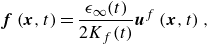 \begin{equation} \boldsymbol {f}\left (\boldsymbol {x},t\right )=\frac {\epsilon _{\infty }(t)}{2K_{f}(t)}\boldsymbol {u}^{f}\left (\boldsymbol {x},t\right ), \end{equation}
where
 $K_{f}(t)=\langle \boldsymbol {u}\cdot \boldsymbol {u}^{f}\rangle /2$
is the filtered turbulence kinetic energy. Here,
 $\langle \sim \rangle$
indicates the spatial average. Clearly,
 $\langle \boldsymbol {f}\cdot \boldsymbol {u}\rangle (t) = \epsilon _{\infty }(t)$
, regardless of the filter, and
 $\epsilon =\epsilon _{\infty }$
holds for homogeneous turbulence when the long time average is taken, where we omit
 $t$
for the time-averaged quantity. Using (2.3), the velocity–force correlation term
 $F(r,t)$
can be written as (Lundgren Reference Lundgren2003)
 \begin{equation} F\left (r,t\right )=\frac {2\epsilon _{\infty }(t)}{r^{3}}\frac {\int _{0}^{r}{\rm d}s\ s^{2}\int {\rm d}\boldsymbol {l}\ g\left (\boldsymbol {s}-\boldsymbol {l}\right )Q\left (l,t\right )}{\int {\rm d}\boldsymbol {l}\ g\left (\boldsymbol {l}\right )Q\left (l,t\right )}, \end{equation}
where
 $Q(r,t)=r^{-2}\partial _{r} [r^{3}u^{2}(t)f(r,t) ]$
. Hereafter, we consider the filter of the form
 $\hat {g} (\boldsymbol {k} )= [H (k )-H (k-k_{f} ) ]$
, where
 $H (\sim )$
represents the Heaviside step function and
 $k_{f}$
is the forcing wavenumber. The low-wavenumber forcing has been widely used in previous DNS (Kaneda et al. Reference Kaneda, Ishihara, Yokokawa, Itakura and Uno2003; McComb et al. Reference McComb, Berera, Yoffe and Linkmann2015; Ishihara et al. Reference Ishihara, Morishita, Yokokawa, Uno and Kaneda2017, Reference Ishihara, Kaneda, Morishita, Yokokawa and Uno2020; Kitamura Reference Kitamura2020, Reference Kitamura2021) to study the inherent dynamics of fluid turbulence at small scales. The upper and lower bounds of
 $C_{\epsilon }$
for low-wavenumber forced turbulence were also mathematically investigated by Doering & Petrov (Reference Doering and Petrov2005). By performing an inverse Fourier transform of
 $\hat {g} (\boldsymbol {k} )= [H (k )-H (k-k_{f} ) ]$
, the filter function is given by
 $g (\boldsymbol {x} )=4\pi k_{f}^{2}j_{1} (k_{f}|\boldsymbol {x}| )/|\boldsymbol {x}|$
, where
 $j_{n} (\sim )$
is the spherical Bessel function of the first kind. Lundgren’s linear forcing can be generalised by considering
 $k_{f}\to \infty$
(Lundgren Reference Lundgren2003) and the filter function is given by
 $g(\boldsymbol {x})=(2\pi )^{3}\delta (\boldsymbol {x})$
, where
 $\delta (\boldsymbol {x})$
is a three-dimensional Dirac delta function.
Substituting
 $g(\boldsymbol {x})=4\pi k_{f}^2 j_{1}(k_{f}|\boldsymbol {x}|)/|\boldsymbol {x}|$
into (2.4) and integrating the resulting equation with respect to the angle variables of
 $\boldsymbol {s}$
and
 $l$
,
 $F (r,t )$
can be written as
 \begin{equation} F\left (r,t\right )=-\frac {1}{\pi k_{f}}\frac {u^{2}(t)}{K_{f}(t)}\frac {\epsilon _{\infty }(t)}{r^{3}}\int _{0}^{\infty }{\rm d}s\ s\alpha (k_{f}r,k_{f}s)f\left (s,t\right ), \end{equation}
with
 \begin{equation} \alpha (r,s)=rs\left [2j_{0}\left (r\right )j_{0}\left (s\right )-j_{0}\left (r+s\right )-j_{0}\left (r-s\right )\right ]. \end{equation}
Integrating (2.1) with respect to
 $r$
from
 $0$
to
 $\infty$
, and using
 ${\rm d}u^{2}(t)/{\rm d}t=2/3 (-\epsilon (t) +\epsilon _{\infty }(t) )$
,
 $C_{\epsilon }(t)$
can be written as
 \begin{equation} C_{\epsilon }(t)=-\frac {3}{2}\alpha _{f}(t)\left [\int _{0}^{\infty }{\rm d}r\ N\left (r,t\right )+\frac {2\nu }{u(t)}\int _{0}^{\infty }{\rm d}r\ D\left (r,t\right )-\frac {1}{u(t)}\frac {{\rm d}L(t)}{{\rm d}t}\right ]=\alpha _{f}(t)\tilde {C}_{\epsilon }(t), \end{equation}
where
 $\alpha _{f}(t)$
is a dependent function of the forcing given by
 \begin{equation} \alpha _{f}(t)=\left [1-\frac {\epsilon _{\infty }(t)}{\epsilon (t)}+\frac {\epsilon _{\infty }(t)L_{f}(t)}{\epsilon (t) L(t)}\right ]^{-1}, \end{equation}
where
 $L_{f}(t)=3\pi /(4K_{f}(t))\int _{0}^{k_{f}}{\rm d}k\ E(k,t)/k$
is the forced integral length scale and
 $E (k,t )$
is the energy spectrum. The above equation is an exact expression derived from the forced KHE and is the same form even for the stochastic forcing.
2.2. Stochastic forcing
Next, we consider the stirring force, assumed to be delta-correlated in time, obeying a Gaussian statistics and a two-point two-time correlation function given by
 \begin{equation} \left \langle \hat {f}_{i}\left (\boldsymbol {k},t\right )\hat {f}_{j}\left (\boldsymbol {p},s\right )\right \rangle =\frac {F\left (k\right )}{4\pi k^{2}}P_{ij}\left (\boldsymbol {k}\right )\delta \left (\boldsymbol {k}+\boldsymbol {p}\right )\delta \left (t-s\right ), \end{equation}
where
 $\,\hat {\boldsymbol {\!f}}$
is the Fourier coefficient of
 $\boldsymbol {f}$
,
 $P_{ij} (\boldsymbol {k} )=\delta _{ij}-k_{i}k_{j}/k^{2}$
is the solenoidal projection operator,
 $\delta _{ij}$
is the Kronecker delta and
 $F (k )$
is the forcing spectrum satisfying
 $\int _{0}^{\infty }{\rm d}k\ F (k )=\epsilon _{\infty }$
. Here,
 $\langle \sim \rangle$
indicates that the average is taken over the different realisation of the random forcing. The Gaussian random forcing, introduced into the turbulence theory by Novikov (Reference Novikov1965), was used to study the four-fifths law from the theoretical framework (Moisy, Tabeling & Willaime Reference Moisy, Tabeling and Willaime1999; Antonia & Burattini Reference Antonia and Burattini2006) and has been widely used in previous DNS (Alvelius Reference Alvelius1999; Fukayama et al. Reference Fukayama, Oyamada, Nakano, Gotoh and Yamamoto2000; Gotoh, Fukayama & Nakano Reference Gotoh, Fukayama and Nakano2002).
Using the Furutsu–Novikov–Donsker formula (Novikov Reference Novikov1965)
 \begin{equation} \left \langle \hat {f}_{i}\left (\boldsymbol {k},t\right )R\left [\,\hat {\boldsymbol {\!f}}\right ]\right \rangle =\int {\rm d}\boldsymbol {k}'\ \int _{-\infty }^{\infty }{\rm d}s'\ \left \langle \hat {f}_{i}\left (\boldsymbol {k},t\right )\hat {f}_{j}\left (\boldsymbol {k}',s'\right )\right \rangle \left \langle \frac {\delta R\left [\,\hat {\boldsymbol {\!f}}\right ]}{\delta \hat {f}_{j}\left (\boldsymbol {k}',s'\right )}\right \rangle , \end{equation}
where
 $R [\,\hat {\boldsymbol {\!f}} ]$
is any function of
 $\,\hat {\boldsymbol {\!f}}$
and
 $\delta /\delta \,\hat {\boldsymbol {\!f}}$
denotes the function derivative, we have
 \begin{equation} \left \langle \hat {f}_{i}\left (\boldsymbol {k},t\right )\hat {u}_{j}\left (\boldsymbol {p},s\right )\right \rangle =\begin{cases} \frac {F\left (k\right )}{8\pi k^{2}}P_{ij}\left (\boldsymbol {k}\right )\delta \left (\boldsymbol {k}+\boldsymbol {p}\right ) & (t=s), \\ 0 & (t\gt s). \end{cases} \end{equation}
Using (2.2) and (2.11),
 $F (r )$
can be written as
 \begin{equation} F\left (r\right )=2\int _{0}^{\infty }{\rm d}k\ \frac {j_{1}\left (kr\right )}{kr}F\left (k\right ). \end{equation}
Using
 $F (r )$
given by (2.12) and integrating (2.1) with respect to
 $r$
from
 $0$
to
 $\infty$
,
 $C_{\epsilon }$
is the same form as (2.7) and (2.8). However, the difference appears in the forcing integral length scale, and
 $L_{f}$
in the stochastic forcing is given by
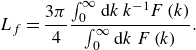 \begin{equation} L_{f}=\frac {3\pi }{4}\frac {\int _{0}^{\infty }{\rm d}k\ k^{-1}F\left (k\right )}{\int _{0}^{\infty }{\rm d}k\ F\left (k\right )}. \end{equation}
The explicit effect of forcing on
 $C_{\epsilon }$
in steady forced turbulence appears only for
 $L_{f}$
, and the same is true even for general forcing (see Appendix A.3) and the homogeneous strain and/or shear-driven turbulence (see Appendix A.4).
2.3.
 $Re_{\lambda }$
dependence of
$C_{\epsilon }$


First, we consider the
 $Re_{\lambda }$
dependence of
 $C_{\epsilon }$
for steady forced turbulence. When turbulence is forced at a constant energy injection rate over relatively large scales, the turbulence reaches a statistically steady state where the energy injection rate balances the energy dissipation rate. The discussion then becomes simpler as the unsteady term can be dropped ideally. In practice, ergodicity is used based on the time stationarity and the time average is used, noting that (2.7) is only valid for the ensemble average. Also note that
 $\epsilon L/u^{3}\neq \lim _{T\to \infty }T^{-1}\int _{0}^{T}{\rm d}t\ \epsilon (t)L(t)/u^3(t)$
, where the variable without explicit description of
 $t$
implies the time-averaged quantity. For the sake of mathematical accuracy, we restart the derivation of
 $C_{\epsilon }\equiv \epsilon L/u^3$
from (2.1). Taking the long-time average with respect to (2.1), integrating the resulting equation with respect to
 $r$
from
 $0$
to
 $\infty$
and multiplying the resulting equation by
 $3L/(2L_{f}u^3)$
,
 $C_{\epsilon }$
can be written as
 \begin{equation} C_{\epsilon }=-\frac {3}{2}\alpha _{f}\left [\int _{0}^{\infty }{\rm d}r\ N\left (r\right )+\frac {2\nu }{u}\int _{0}^{\infty }{\rm d}r\ D\left (r\right )\right ], \end{equation}
where
 $\alpha _{f}=L/L_{f}$
,
 $K (r )=\langle u_{L}^2 (\boldsymbol {0} )u_{L} (\boldsymbol {r} )\rangle /u^3$
and
 $f (r )=\langle u_{L} (\boldsymbol {0} )u_{L} (\boldsymbol {r} )\rangle /u^2$
.
By introducing the non-dimensional length
 $\rho =r/L$
,
 $C_{\epsilon }$
can be written as
 \begin{equation} C_{\epsilon }=-\frac {3}{2}\alpha _{f}\left [\int _{0}^{\infty }{\rm d}\rho \ \tilde {N}(\rho )+\frac {2}{Re_{L}}\int _{0}^{\infty }{\rm d}\rho \ \tilde {D}(\rho )\right ], \end{equation}
where
 $Re_{L}=uL/\nu$
is the Reynolds number based on the integral length scale,
 $\tilde {N} (\rho )=\rho ^{-4}d [\rho ^{4}K (\rho L ) ]/{\rm d}\rho$
and
 $\tilde {D}(\rho )=\rho ^{-4}{\rm d} [\rho ^{4}{\rm d}f (\rho L )/{\rm d}\rho ]/{\rm d}\rho$
, which can be written in the compact form
 $C_{\epsilon }=\alpha _{f} [C_{\mathcal {N}}+C_{\mathcal {D}}/Re_{L} ]$
. It should be noted that the above expression is almost the same as the scale-dependent expression of McComb et al. (Reference McComb, Berera, Yoffe and Linkmann2015), but the uncertainty due to the scale-dependence is removed in (2.15), i.e. one-point statistics in the present study and two-point statistics by McComb et al. (Reference McComb, Berera, Yoffe and Linkmann2015). Furthermore, the influence of forcing, i.e.
 $\alpha _{f}$
, is not included in their theory.
Substituting the relation
 $Re_{L}=C_{\epsilon }Re_{\lambda }^{2}/15$
into (2.15), we obtain the quadratic equation with respect to
 $C_{\epsilon }$
of the form
 $C_{\epsilon }=\alpha _{f} [C_{\mathcal {N}}+15C_{\mathcal {D}}/ (C_{\epsilon }Re_{\lambda }^{2} ) ]$
, and the solution is expressed as
 \begin{equation} C_{\epsilon }=A\left [1+\sqrt {1+\left (\frac {B}{Re_{\lambda }}\right )^{2}}\right ], \end{equation}
where
 $A$
and
 $B$
are given as
 $A=\alpha _{f}C_{\mathcal {N}}/2$
and
 $B=2\sqrt {15C_{\mathcal {D}}/\alpha _{f}}/C_{\mathcal {N}}$
. It should be noted that the above expression is the same as the upper bound derived by Doering & Foias (Reference Doering and Foias2002) and the scale-dependent expression of McComb et al. (Reference McComb, Berera, Yoffe and Linkmann2015). It is clear from (2.16) that the value of
 $C_{\epsilon }$
depends on the forcing because of the explicit appearance of
 $\alpha _{f}$
in
 $C_{\epsilon }$
, and the present results theoretically support the observation made by Sreenivasan (Reference Sreenivasan1998). Furthermore, it is conjectured that the dissipation anomaly originates from the Reynolds number independence of the nonlinear energy transfer described by
 $C_{\mathcal {N}}$
at sufficiently high Reynolds numbers. Further discussion requires the closure hypothesis and, therefore, it is left for future studies, and the numerical evidence for
 $C_{\mathcal {N}}\approx \textrm {const.}$
at sufficiently high Reynolds number is shown later.
Next, we consider
 $C_{\epsilon }$
in decaying turbulence. Starting from (2.7), with
 $\epsilon _{\infty }=0$
,
 $C_{\epsilon }(t)$
in decaying turbulence can be written as
 \begin{equation} C_{\epsilon }(t)=C_{\mathcal {N}}(t)+\frac {\nu _{t}(t)/\nu }{Re_{L}(t)}+\frac {C_{\mathcal {D}}(t)}{Re_{L}(t)}, \end{equation}
where
 $\nu _{t}(t)=(3/4){\rm d}L^{2}(t)/{\rm d}t$
. Substituting
 $Re_{L}(t)=C_{\epsilon }(t)Re_{\lambda }^{2}(t)/15$
into the above relation, we obtain the same expression as (2.16), but
 $A=C_{\mathcal {N}}(t)/2$
and
 $B=2\sqrt {15(C_{\mathcal {D}}(t)+\nu _{t}(t)/\nu )}/C_{\mathcal {N}}(t)$
. In the subsequent following discussions, we consider freely decaying turbulence with an initial condition of forced turbulence. Since
 $C_{\mathcal {D}}/Re_{L}$
is negligible for forced turbulence at sufficiently high Reynolds numbers, we assume
 $\nu _{t}(t)/\nu \gg C_{\mathcal {D}}(t)$
even for decaying turbulence (the supporting experimental evidence in regular grid turbulence for
 $Re_{\lambda }\geqslant 50$
is shown by Sreenivasan (Reference Sreenivasan1984)) and therefore simply (2.17) as
 $C_{\epsilon }(t)=C_{\mathcal {N}}(t)+ (\nu _{t}(t)/\nu )/Re_{L}(t)$
. As with forced turbulence, we assume that
 $C_{\mathcal {N}}\approx \textrm {const.}$
also holds even for decaying turbulence at sufficiently high Reynolds numbers.
2.3.1. Non-equilibrium dissipation law
Using the non-equilibrium dissipation law of the form
 $C_{\epsilon }(t)=\zeta (\sqrt {Re_{L}(0)}/Re_{\lambda }(t) )$
, where
 $\zeta =C_{\epsilon }(0)Re_{\lambda }(0)/\sqrt {Re_{L}(0)}$
, and the kinematic relation
 $Re_{L}(t)=C_{\epsilon }(t)Re_{\lambda }^{2}(t)/15$
, and taking the time derivative of
 $C_{\epsilon }(t)=C_{\mathcal {N}}(t)+ (\nu _{t}(t)/\nu )/Re_{L}(t)$
, we have
 \begin{equation} \frac {d}{{\rm d}t}\left (\frac {\nu _{t}(t)}{\nu }\right )=\frac {1}{Re_{\lambda }(t)}\frac {{\rm d}Re_{\lambda }(t)}{{\rm d}t}\left [\frac {\nu _{t}(t)}{\nu }-\frac {\zeta ^2Re_{L}(0)}{15}\right ], \end{equation}
where
 $C_{\mathcal {N}}(t)\approx \textrm {const.}$
was used. Using
 $C_{\epsilon }(t)=C_{\mathcal {N}}(t)+ (\nu _{t}(t)/\nu )/Re_{L}(t)$
and
 $L(t)/\lambda (t)=L(0)/\lambda (0)$
, the term in the bracket of the right-hand side satisfies the inequality
 \begin{equation} \frac {\nu _{t}(t)}{\nu }-\frac {\zeta ^2 Re_{L}(0)}{15}=15\frac {Re_{L}^2(t)}{Re_{\lambda }^2(t)}-Re_{L}(t)C_{\mathcal {N}}(t)-15\frac {Re_{L}^2(0)}{Re_{\lambda }^2(0)}=-Re_{L}(t)C_{\mathcal {N}}(t) \lt 0. \end{equation}
Hence, the transient regime in which the non-equilibrium dissipation law is observed satisfies
 $d (\nu _{t}(t)/\nu )/{\rm d}t\gt 0$
because
 $dRe_{\lambda }/{\rm d}t\lt 0$
. In other words, the non-equilibrium dissipation law holds before the critical time
 $t_{c}$
which is defined as the time when
 $d (\nu _{t}(t)/\nu )/{\rm d}t$
stops growing, and its physical interpretation is being considered as the cross-over time changing from the non-equilibrium dissipation law to the classical dissipation law (Goto & Vassilicos Reference Goto and Vassilicos2016).
2.3.2. Classical dissipation law
From the above discussion, it can be deduced that the classical dissipation law
 $C_{\epsilon }\approx \textrm {const.}$
is, in contrast, observed at
 $t\gt t_{c}$
. The numerical evidence is shown by Goto & Vassilicos (Reference Goto and Vassilicos2016) and in our results shown in later. Note that the classical dissipation law found for
 $t\gt t_{c}$
corresponds to what Goto & Vassilicos (Reference Goto and Vassilicos2016) call a balanced non-equilibrium dissipation law.
For decaying turbulence such as Saffman and Batchelor turbulence, the turbulent kinetic energy decay law and growth of the integral length scale may be given by
 $u^2(t)\propto t^{-2 (n+1 )/ (n+3 )}$
and
 $L(t)\propto t^{2/ (n+3 )}$
(Krogstad & Davidson Reference Krogstad and Davidson2010), where
 $n$
is the spectral slope of the energy spectrum at low wavenumber
 $E (k\to 0 )\propto k^{n}$
. Hence,
 $C_{\epsilon }\approx \textrm {const.}$
implies
 $C_{\mathcal {N}}\approx \textrm {const.}$
given that
 $Re_{L}(t)\propto \nu _{t}(t)/\nu$
follows from the above power laws. Further,
 $C_{\epsilon }(t)$
in Saffman and Batchelor turbulence is larger than that in forced turbulence, as long as the Reynolds number is sufficiently large and
 $C_{\mathcal {N}}(t)$
is approximately constant and insensitive to decaying and forced turbulence, when
 $\alpha _{f}(t)\leqslant 1$
(
 $\alpha _{f}\leqslant 1$
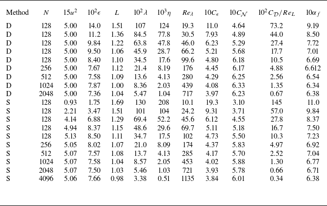
is valid for the low-wavenumber forced turbulence at sufficiently high Reynolds number; see table 1 in Appendix B) due to the presence of
 $\alpha _{d}(t)$
. The present explanation is different from the explanation based on the spectral imbalance which takes into account of the cascade time (Bos, Shao & Bertoglio Reference Bos, Shao and Bertoglio2007) with regards to why
 $C_{\epsilon }$
in decaying turbulence takes a larger value than that of forced turbulence.
Forced turbulence characteristics in DNS. The characters D and S in the method indicate deterministic and stochastic forcing methods. The statistical quantities presented here are averaged over space and time.
3. Numerical results
To validate theoretical analyses, we simulated forced and decaying turbulence. The main purpose of the DNS is to confirm the Reynolds number independence of
 $C_{\mathcal {N}}$
at sufficiently high Reynolds number and the non-equilibrium dissipation law originating from the imbalance
 $u^{-1}{\rm d}L/{\rm d}t\neq \textrm {const.}$
. We solved the incompressible Navier–Stokes equation using the spectral method with full de-aliasing. The computational grid size is
 $128^{3}$
at the minimum and
 $2048^{3}$
for deterministic forcing, and
 $4096^3$
for stochastic forcing at the maximum. The numerical details were almost the same as those in our previous studies (Kitamura Reference Kitamura2020, Reference Kitamura2021) and we stored 100 snapshots of fully developed forced turbulence for the data analyses (35 snapshots for
 $4096^3$
), where each snapshot was sufficiently separated in time. Although the deterministic and stochastic forcing methods used in this study differ slightly from (2.3) and (2.9), in that the energy injection rate was controlled, these differences do not influence the nature of the problem. The details of numerical method and information are shown in Appendix B. We also performed DNS of freely decaying turbulence using snapshots of the aforementioned deterministic forced turbulence as initial conditions. We computed four different initial Reynolds numbers, and five simulations were performed for each case to obtain an ensemble average.
Compensated energy spectra and energy fluxes normalised by the Kolmogorov variables for (
 $a$
) forced turbulence and (
 $b$
) decaying turbulence. Only results of stochastic forced turbulence with
 $Re_{\lambda }\geqslant \mathcal {O}(10^2)$
are shown in panel (
 $a$
), and only results of decaying turbulence with the initially highest Reynolds number are shown in panel (
 $b$
). The shaded regions represent the standard deviation. The compensated energy spectra of panel
 $(b$
) are shifted upwards by an addition of 0.5 for clarity and are plotted every
 $\Delta t/T_{L}(0)=0.18$
from
 $t/T_{L}(0)=0.0018$
, where
 $\Delta t$
is the time interval of the output. The red and blue colour bars represent
 $t/T_{L}(0)$
, where the darker colour represents the result at an earlier stage of decay and the lighter colour represents the result some time after decay.
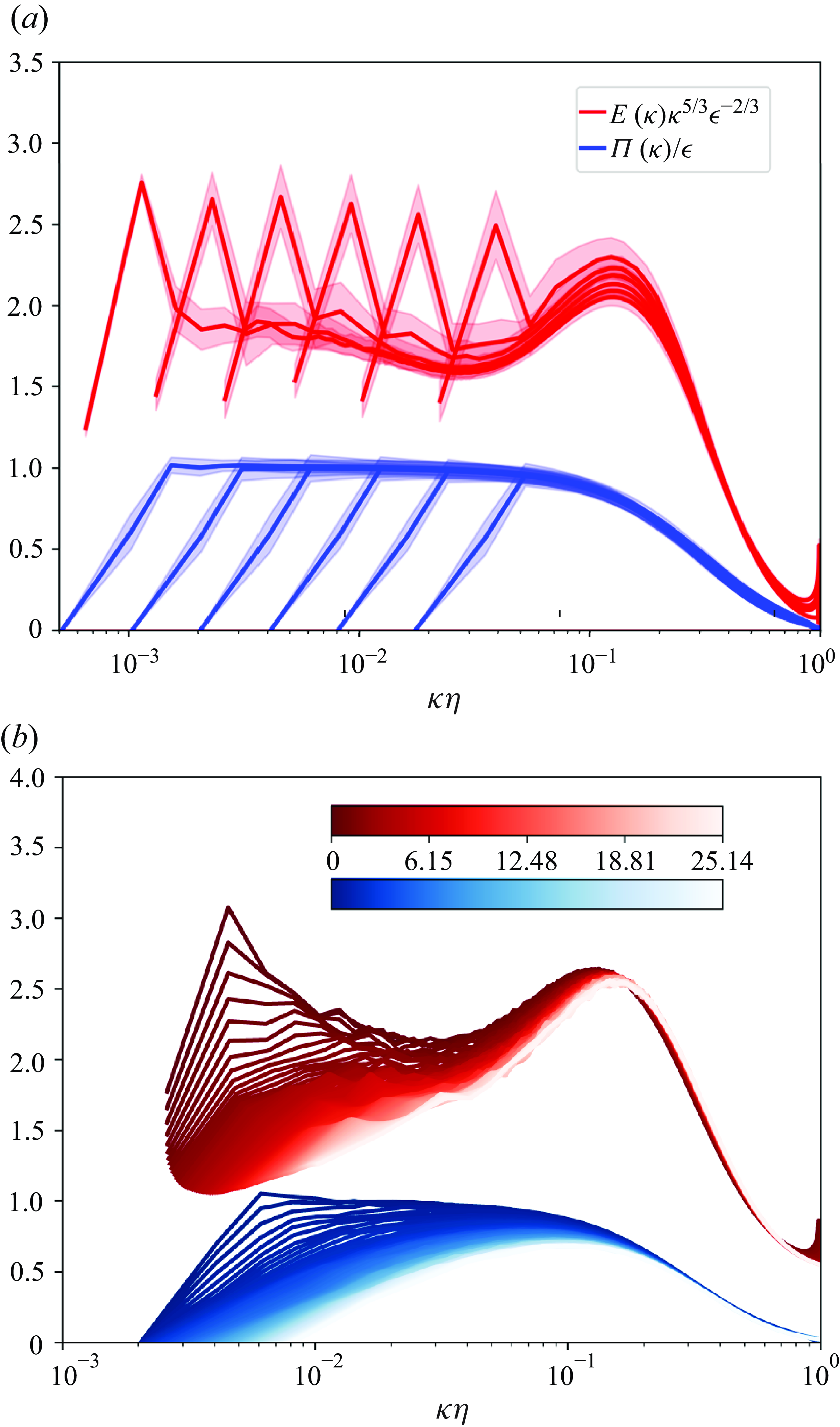
Figures 1(
 $a$
) and 1(
 $b$
) show the compensated energy spectra and energy fluxes for forced and decaying turbulence, where the differences are negligible between forcing schemes and hence the results of deterministic forced turbulence are omitted. The energy spectra and energy fluxes are normalised by the Kolmogorov variables. We first observe the energy spectrum and energy flux for forced turbulence. As in the previous studies of the high-Reynolds-number forced turbulence (Kaneda et al. Reference Kaneda, Ishihara, Yokokawa, Itakura and Uno2003; Ishihara et al. Reference Ishihara, Morishita, Yokokawa, Uno and Kaneda2017), the spectral bump is observed for all cases, and the wavenumber taking the maximum value of the spectral bump has a weak Reynolds number dependence and is
 $k\eta \approx 0.126$
, which is the lower bound of inertial subrange expected from the four-fifths law, i.e.
 $2\pi \eta /\lambda \approx 0.094$
, for the highest Reynolds number in this study. Furthermore, the tilted regions with a small negative slope are observed as done by Kaneda et al. (Reference Kaneda, Ishihara, Yokokawa, Itakura and Uno2003) and Ishihara et al. (Reference Ishihara, Morishita, Yokokawa, Uno and Kaneda2017) for
 $0.0055 \lt k\eta \lt 0.02$
, and the slope is close to −0.09. The slope in the present result is close to the previous studies (Gotoh & Watanabe Reference Gotoh and Watanabe2015; Ishihara et al. Reference Ishihara, Morishita, Yokokawa, Uno and Kaneda2017). For
 $Re_{\lambda }\sim \mathcal {O} (10^2 )$
, we cannot see the plateau in the compensated energy spectrum, however, a slight plateau is observed at the highest Reynolds number. Hence, the Kolmogorov constant
 $C_{K}$
is computed over the range of wavenumbers
 $0.0020\lt k\eta \lt 0.0055$
for the highest Reynolds number and it is
 $C_{K}=1.85\pm 0.03$
. The value is close to
 $1.83\pm 0.01$
reported by Gotoh & Watanabe (Reference Gotoh and Watanabe2015). The energy fluxes are equal to the energy dissipation rate in the wavenumbers
 $k/k_{f}\lt k\eta \ll 2\pi \eta /\lambda \ll 1$
.
We next observe the energy spectrum and energy flux for decaying turbulence. As shown in figure 1(
 $b$
), the energy spectrum and energy flux collapse well at the higher wavenumbers, and the differences in the temporal evolutions of energy spectrum and energy flux are mainly observed in the low wavenumber range, bordering the spectral bump. Given that the four-fifths law holds in the limit,
 $\lim _{r/\lambda \to \infty }\langle \delta u_{L}^3\rangle / (\epsilon r )=-4/5$
, the lower bound of the inertial subrange is at least
 $r=\lambda$
(Nie & Tanveer Reference Nie and Tanveer1999). Therefore, the inertial subrange in spectral space is
 $k\leqslant 2\pi /\lambda$
, just around the spectral bump as discussed above. Thus, Kolmogorov’s theory in terms of the universality of the small-scale structures at the dissipation range, i.e.
 $k \gg 2\pi /\lambda$
, is not violated at least for the third-order structure function even for the transient regime in which the non-equilibrium dissipation law is observed. However, energy damping is mainly observed for the large-scale structures. For example, the most amount of energy for the large-scale structures is lost within the eddy turnover time as understood from the temporal changes in the peak of the compensated energy spectra around
 $k\approx k_{f}$
. This fast drain of the energy from the large-scale structures is peculiar to the region in which the non-equilibrium dissipation law is observed. In other words, the decrease of energy at the peak of the energy containing range is responsible for the time variation of
 $u^{-1}(t){\rm d}L(t)/{\rm d}t$
. Then, the spectral slope of the energy spectrum becomes shallower than
 $k^{-\frac {5}{3}}$
after an eddy turnover time. Similarly,
 $\Pi (k,t )=\epsilon (t)$
does not hold at the later time in spite of moderate Reynolds number
 $Re_{\lambda }\sim 10^2$
. These observations may be due to the insufficient Reynolds number to observe the inertial subrange for decaying turbulence rather than the phenomenon peculiar to the transient regime in which the non-equilibrium dissipation law is observed. It is noted that the shallower one-dimensional energy spectrum has been observed in experiments at relatively high Reynolds number (Saddoughi & Veeravalli Reference Saddoughi and Veeravalli1994) and the approach to four-fifths law is different for decaying and forced turbulence (Antonia & Burattini Reference Antonia and Burattini2006), e.g. a much higher Reynolds number is required for decaying turbulence to have the well-defined power law behaviours in the inertial subrange.
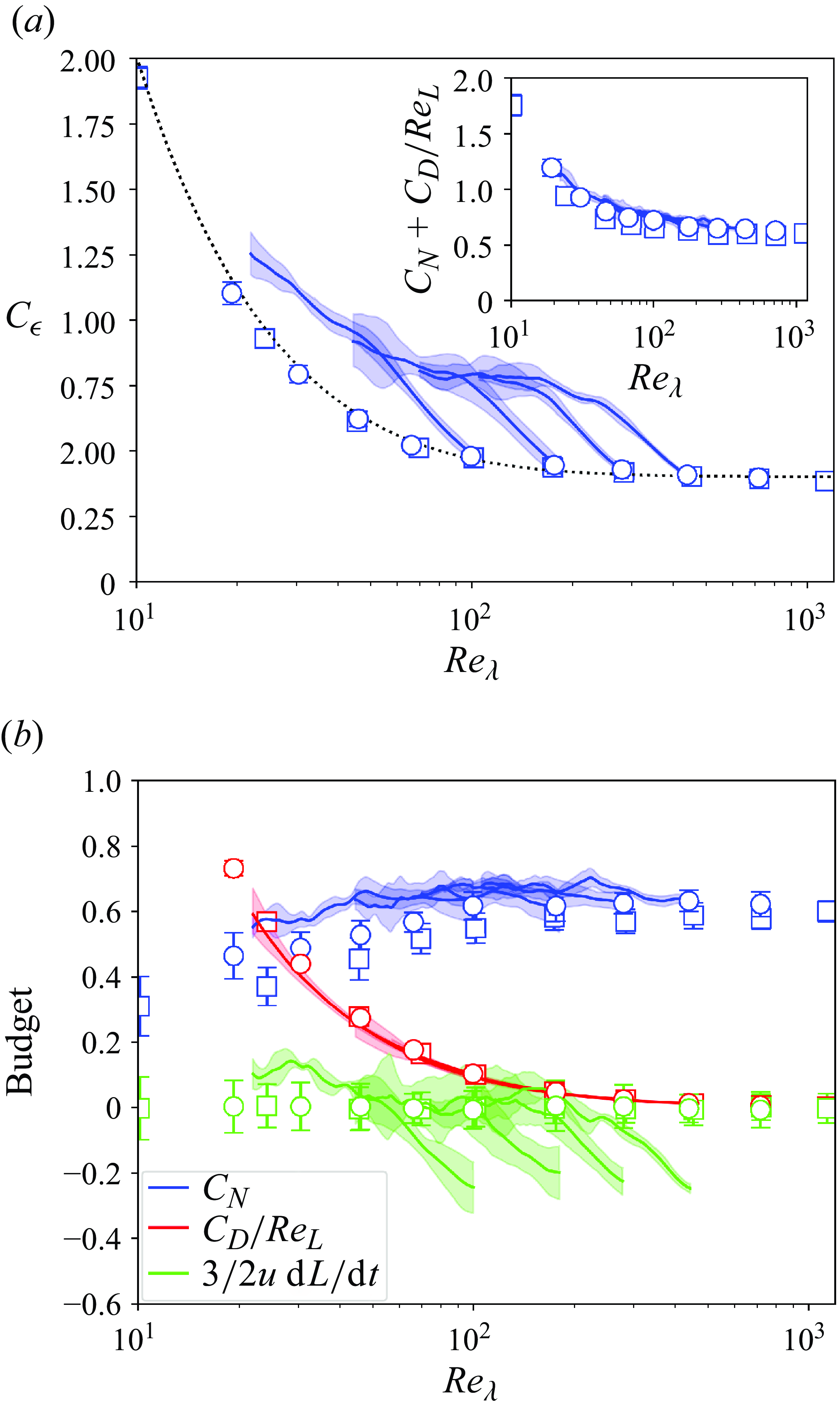
(
 $a$
) Normalised energy dissipation rate
 $C_{\epsilon }$
versus Reynolds number
 $Re_{\lambda }$
with
 $\pm \sigma$
uncertainty, where
 $\sigma ^2$
is the mean squared error of the difference between the instantaneous quantity and ensemble average. The blue open circles, blue open squares and blue lines represent the results for deterministic-forced, stochastic-forced and decaying turbulence, respectively. Inset shows
 $C_{\mathcal {N}}+C_{\mathcal {D}}/Re_{L}$
versus
 $Re_{\lambda }$
. (
 $b$
) Budget for
 $\tilde {C}_{\epsilon }$
, where the open circles, open squares and solid lines represent the terms in the budget of
 $\tilde {C}_{\epsilon }$
for the deterministic-forced, stochastic-forced and decaying turbulence. The same colour represents the same term and is defined in the legend.
The numerical methods of the statistical quantities are shown in Appendix B. The statistical quantities are defined so as to provide the unified interpretation regardless of decaying and forced turbulence. In the following discussion, we rewrite (2.7) in the simple form
 \begin{equation} C_{\epsilon }(t)=\alpha _{f}(t)\left [C_{\mathcal {N}}(t)+\frac {C_{\mathcal {D}}(t)}{Re_{L}(t)}+\frac {3}{2u(t)}\frac {{\rm d}L(t)}{{\rm d}t}\right ]=\alpha _{f}(t)\tilde {C}_{\epsilon }(t). \end{equation}
Figure 2(
 $a$
) shows the relation between
 $C_{\epsilon }$
and
 $Re_{\lambda }$
together with functional form (2.16) with
 $A=0.2$
and
 $B=90$
for the reference curve in forced turbulence. Here,
 $C_{\epsilon }$
for forced turbulence asymptotes to a constant value (
 ${\sim} 0.4$
) with an increase in
 $Re_{\lambda }$
and the effect of forcing on
 $C_{\epsilon }$
is negligibly small, whereas that for decaying turbulence is a dependent function of
 $Re_{\lambda }$
during a transition regime characterised by
 $u^{-1}{\rm d}L/{\rm d}t\neq \textrm {const.}$
and this asymptotes a constant value (
 ${\sim} 0.8$
) for the decaying regime characterised by
 $u^{-1}{\rm d}L/{\rm d}t\approx \textrm {const.}$
. The inset of figure 2(
 $a$
) shows
 $C_{\mathcal {N}}+C_{\mathcal {D}}/Re_{L}$
versus
 $Re_{\lambda }$
, which collapses well irrespective of forced and decaying turbulence. This implies that the bare dynamics of fluid turbulence may not be substantially altered by the presence of and type of forcing. Furthermore, our results suggest that the following form of non-dimensionalisation is useful in flow fields where external forces are present:
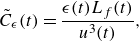 \begin{equation} \tilde {C}_{\epsilon }(t)=\frac {\epsilon (t) L_{f}(t)}{u^3(t)}, \end{equation}
since
 $C_{\mathcal {N}}$
explicitly appears. Pearson, Krogstad & van de Water (Reference Pearson, Krogstad and van de Water2002) show that it is better collapsed by using the predominant energy scale
 $L_{\mathcal {P}}$
instead of
 $L$
in the dimensionless formulation of
 $\epsilon$
. Interpreted as
 $L_{f}\propto L_{\mathcal {P}}$
and applied to our theory, their experimental results can be interpreted as experimental evidence that
 $C_{\mathcal {N}}$
is indeed constant in high-Reynolds-number turbulence. The budgets shown in figure 2(
 $b$
),
 $C_{\mathcal {N}}$
and
 $C_{\mathcal {D}}/Re_{L}$
, are almost the same for forced and decaying turbulence. However, there are the weak Reynolds number and the weak forcing dependencies for
 $C_{\mathcal {N}}$
, and the asymptotic value based on the highest Reynolds number result is
 $C_{\mathcal {N}}=0.60\pm 0.03$
. For
 $Re_{\lambda }\leqslant \mathcal {O} (10^2 )$
, the decreasing behaviour of
 $C_{\mathcal {N}}$
with respect to
 $Re_{\lambda }$
is observed, and this is quite natural since the nonlinearity decreases with the decrease of Reynolds number, e.g. it is expected that
 $C_{\mathcal {N}}=0$
for
 $Re_{\lambda }=0$
.
Meanwhile, the origin of
 $C_{\epsilon }\neq \textrm {const.}$
originates from the imbalance between
 $u$
and
 ${\rm d}L/{\rm d}t$
, as predicted by (3.1) with
 $\alpha _{f}=1$
. These numerical results are consistent with the aforementioned theoretical analyses. These facts suggest that
 $C_{\mathcal {N}}$
does not depend much on the flow field at high Reynolds number, and the reason why
 $C_{\epsilon }\neq \textrm {const.}$
is explained from
 $\alpha _{f}(t)$
and
 $u^{-1}(t){\rm d}L(t)/{\rm d}t$
, as understood from (3.1). Two things must be noted here. The first is that in practical calculations, instead of ensemble averages, the discussion is often based on spatial averages only, but due to their finite size, fluctuations in the energy injection and dissipation lead a certain amount of imbalance, and care must be taken with the meaning of the averages used in (3.1). Second, it is considered that whether the reason for
 $C_{\epsilon }\neq \textrm {const.}$
comes from
 $\alpha _{f}(t)$
or
 $u^{-1}(t){\rm d}L(t)/{\rm d}t$
or both depends on the flow field in the case of a flow field in the presence of driving force such as the mean velocity gradient. Note that the non-equilibrium dissipation law originates from
 $u^{-1}(t){\rm d}L(t)/{\rm d}t$
for freely decaying turbulence since
 $\alpha _{f}=1$
. More specifically, when considering inhomogeneous turbulence, it is necessary to construct a theory from the Kármán–Howarth–Monin–Hill equation, i.e. integrated form of the KHMH equation, but this may lead to a more complicated Reynolds number dependence of
 $C_{\epsilon }$
because the advection, production and diffusion terms appear in the parts of
 $\alpha _{f}(t)$
and
 $u^{-1}(t){\rm d}L(t)/{\rm d}t$
. The intensive study on the inhomogeneous and anisotropic turbulence will be reported in more detail elsewhere in the future.
 $L/\lambda$
versus
 $Re_{\lambda }$
with
 $\pm \sigma$
uncertainty. Also included are
 $L/\lambda =(2/75)Re_{\lambda }$
for a reference curve. The symbols are the same as those in figure 2(
 $a$
).
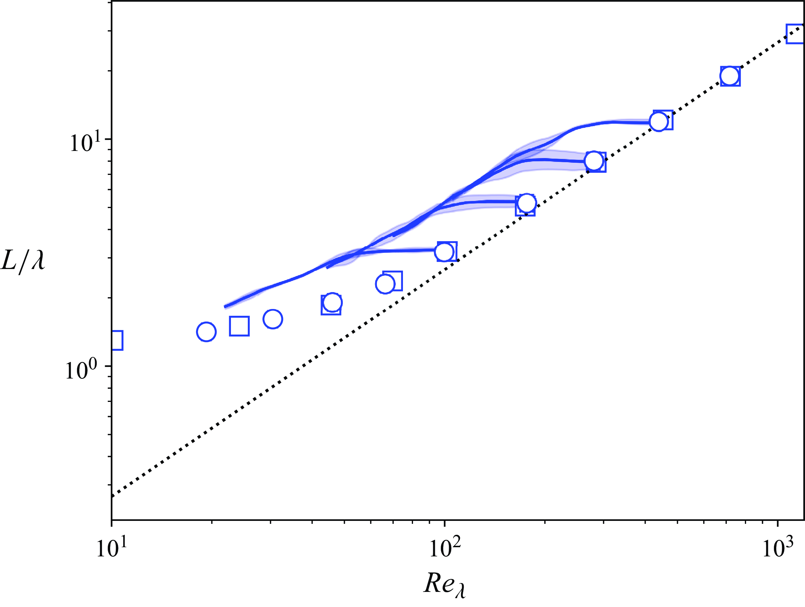
Figure 3 shows the relation between
 $L/\lambda$
and
 $Re_{\lambda }$
together with
 $L/\lambda =(2/75)Re_{\lambda }$
. Here,
 $L/\lambda$
for forced turbulence increases with the increase of the Reynolds number, whereas
 $L/\lambda$
for decaying turbulence remains approximately constant in the transient regime in which the non-equilibrium dissipation law is observed, and
 $L/\lambda$
decreases with the decrease of the Reynolds number for the decaying regime in which the non-equilibrium dissipation law is not observed.
To validate the theoretical analyses in § 2.3, we define the characteristic times. We define
 $t_{g}$
and
 $t_{c}$
as the times when
 $\nu _{t}/\nu$
is zero and
 $\nu _{t}/\nu$
is maximum, according to Goto & Vassilicos (Reference Goto and Vassilicos2016). Further, we introduce
 $t_{n}$
based on theoretical analyses. Since (2.17) implies that the non-equilibrium dissipation law is not determined from
 $\nu _{t}(t)/\nu$
alone, but from the combination of
 $\nu _{t}(t)/\nu$
and
 $Re_{L}(t)$
, we write (2.17) as follows:
 \begin{equation} C_{\epsilon }(t)=C_{\mathcal {N}}(t)+\frac {3}{2u(t)}\frac {{\rm d}L(t)}{{\rm d}t}, \end{equation}
where
 $C_{\mathcal {D}}(t)/Re_{L}(t)$
is neglected since our concern is high-Reynolds-number decaying turbulence. Based on (3.3), the non-equilibrium dissipation law should be determined from
 $(3/2)u^{-1}(t){\rm d}L(t)/{\rm d}t$
only since
 $C_{\mathcal {N}}(t)\approx \textrm {const.}$
. Therefore,
 $t_{n}$
is defined as the first time satisfying
 $d (u^{-1}(t){\rm d}L(t)/{\rm d}t )/{\rm d}t=0$
.
(
 $a$
) Decay of the turbulent kinetic energy for the highest Reynolds number and the dash–dot line represents
 $\propto t^{-1.7}$
for the reference curve, where the inset represents the decay of
 $I(t)$
. (
 $b$
) Change in the integral length scale, where theinset shows the changes in
 $\nu _{t}(t)/\nu$
(solid line) and other related quantities,
 $\zeta ^2Re_{L}(0)/15=(C_{\epsilon }(0)Re_{\lambda }(0))^2/15$
(dash-dotted line),
 $[L(t)/(u^2(t)\nu )]{\rm d}I(t)/{\rm d}t$
(dashed line) and
 $\epsilon (t) L^2(t)/(u^2(t)\nu )$
(dotted line), each normalised to
 $Re_{L}(0)$
. Also marked by stars, diamonds, squares and circles are the results at
 $t=T_{L}(0)$
,
 $t=t_{n}$
,
 $t=t_{g}$
and
 $t=t_{c}$
, respectively.
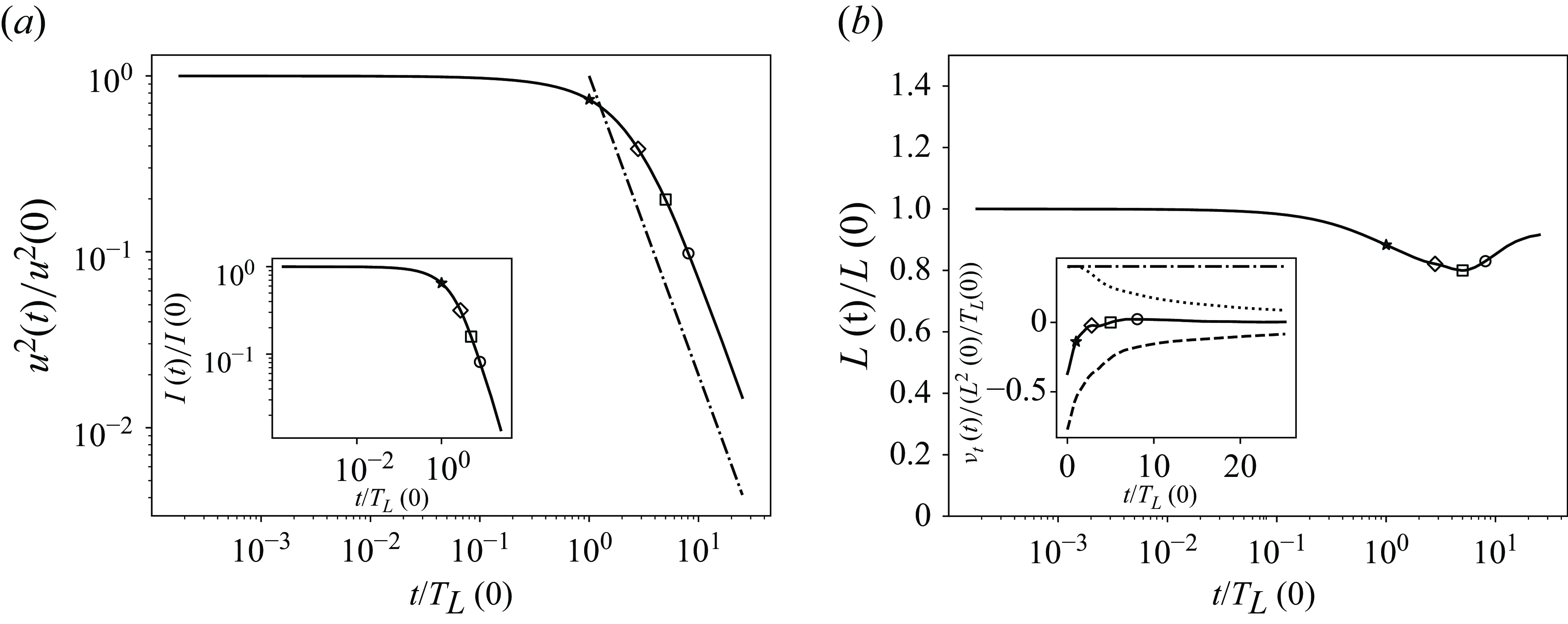
Figure 4(
 $a$
) shows the decay of turbulent kinetic energy and the inset shows the decay of
 $I(t)=u^2(t)\int _{0}^{\infty }{\rm d}r\ f(r,t)$
, where
 $I(t)\propto \int _{0}^{\infty }{\rm d}k\ E(k,t)/k$
is a quantitative measure of the large-scale quantity. As shown in figure 4(
 $a$
), the fast decay of the turbulent kinetic energy is observed for
 $t/T_{L}(0)\gg 1$
. The similar fast decay has been reported for the energy spectrum obeying the Kolmogorov spectrum in the calculation of the eddy-damped quasi-normal Markovian (EDQNM) closure (Lesieur & Ossia Reference Lesieur and Ossia2000) and in the DNS (Yang, Pumir & Xu Reference Yang, Pumir and Xu2018).
Figure 4(
 $b$
) shows the changes in integral length scale and the inset shows the change in
 $\nu _{t}/\nu$
, where
 $\nu _{t}/\nu$
can be decomposed into
 $\nu _{t}/\nu = [L(t)/(u^2(t)\nu ) ]{\rm d}I(t)/{\rm d}t+L^2(t)\epsilon (t)/(u^2(t)\nu )$
. As shown in figure 4(
 $b$
), the integral length scale is approximately constant, but weakly decreasing as a function of time before
 $t=t_{c}$
. Then, the integral length scale evolves in time. The similar evolution of the integral length scale is also reported in the DNS by Yang et al. (Reference Yang, Pumir and Xu2018). The characteristic times except for
 $t_{n}$
are in the order of
 $T_{L}(0)\lt t_{g}\lt t_{c}$
, and
 $t_{n}$
depends on the Reynolds number. As shown in the inset in figure 4(
 $b$
),
 $\nu _{t}/\nu$
is an increasing function until
 $t_{c}$
and a decreasing function after
 $t_{c}$
. The same trend was also shown by Goto & Vassilicos (Reference Goto and Vassilicos2016). Furthermore, our results show that an inequality
 $\nu _{t}(t)/\nu -\zeta ^2Re_{L}(0)/15\lt 0$
holds regardless of the non-equilibrium and classical dissipation laws. Also,
 $\nu _{t}(t)/\nu$
is characterised mainly by
 $ [L(t)/(u^2(t)\nu ) ]{\rm d}I(t)/{\rm d}t$
at
 $t\lt t_{n}$
, which is consistent with very fast decay at large scales as discussed above.
 $C_{\epsilon }/\sqrt {Re_{L}(0)}$
versus
 $Re_{\lambda }$
, where the dotted and dash–dotted lines represent −1 and −15/14 power laws, respectively. The colour is almost the same as that in the energy spectrum shown in figure 1(
 $b$
). The symbols are the same as those in figure 4. The colour bar represents
 $t/T_{L}(0)$
, where the darker colour represents the result at an earlier stage of decay and the lighter colour represents the result some time after decay.
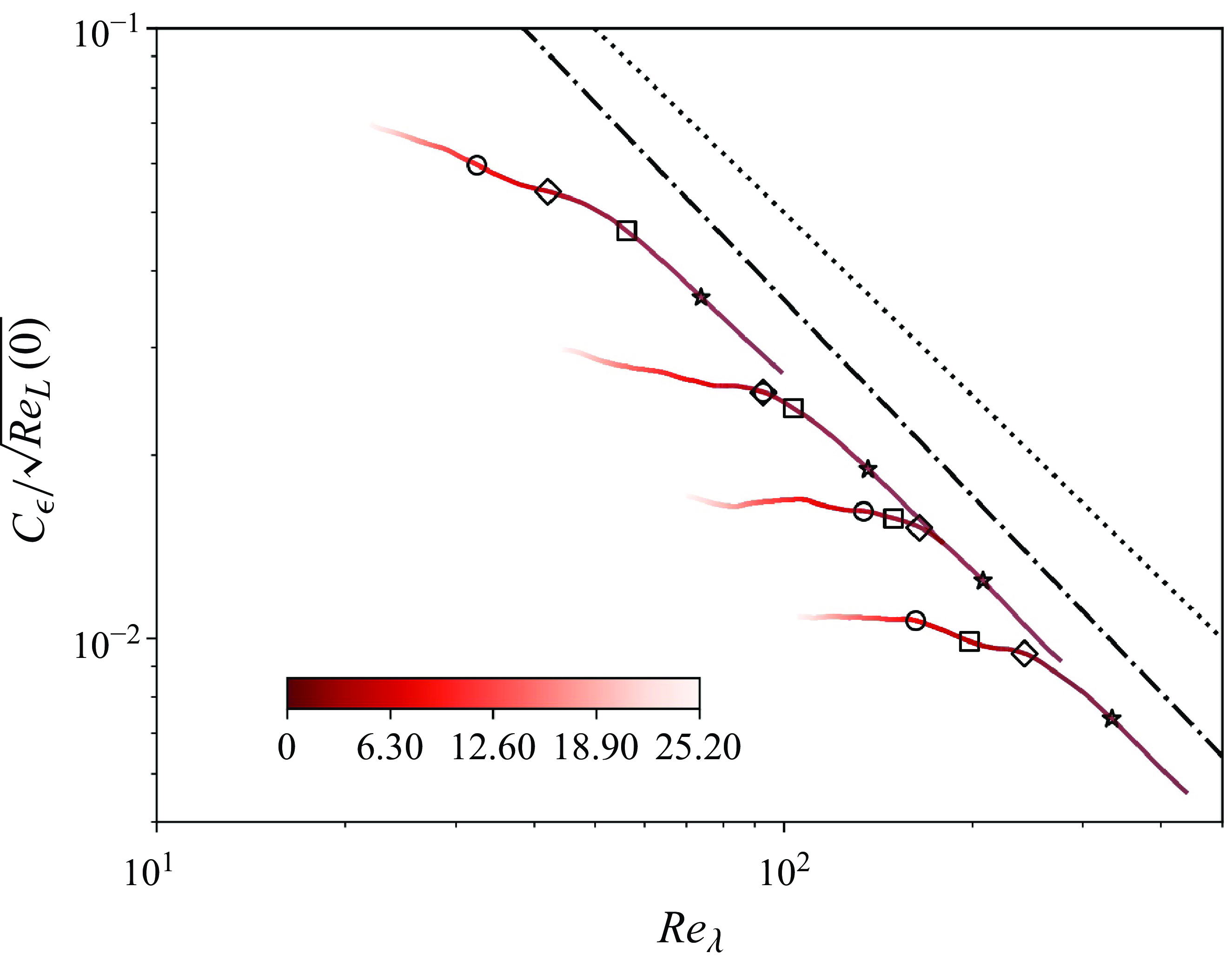
Figure 5 shows the non-equilibrium dissipation law for decaying turbulence. The transient regime obeying
 $C_{\epsilon }/\sqrt {Re_{L}(0)}\propto Re_{\lambda }^{\xi }$
with
 $\xi \approx -1$
is observed at the early stages after turning off the forcing. In this transient regime, the energy at forcing scale rapidly changes as shown in figures 1(
 $b$
) and 4(
 $b$
), and this may be physically interpreted that
 $\nu _{t}(t)=3/4{\rm d}L^2(t)/{\rm d}t$
acts on the large-scale structures as an eddy viscosity to drain the energy. As shown in figure 5, of the several times mentioned above,
 $t_{n}$
is the best predictor of the time at which the non-equilibrium dissipation law holds for high-Reynolds-number turbulence. The reason for the lax estimate at low Reynolds numbers is that
 $C_{\mathcal {D}}(t)/Re_{L}(t)$
has not been taken into account and viscous effects have appeared. Based on our theoretical analyses in § 2.3,
 $t_{C}$
can be classified for regions where non-equilibrium and classical dissipation laws are valid, but it is considered quite natural that there are regions with smooth transitions before and after
 $t_{c}$
, and
 $t_{n}$
may be suited for the classification of the regions in which the non-equilibrium dissipation law is observed. Hence, the imbalance between
 $u(t)$
and
 ${\rm d}L(t)/{\rm d}t$
is more important than
 $\nu _{t}(t)/\nu$
for the non-equilibrium dissipation law.
We lastly comment on
 $C_{\mathcal {N}}(t)\approx \textrm {const.}$
. As is clear from the definition
 $C_{\mathcal {N}}(t)=-(4u^3(t))^{-1}\int _{0}^{\infty }{\rm d}r\ r^{-4}\partial _{r} [r^4\langle \delta u_{L}^3\rangle ]$
,
 $C_{\mathcal {N}}$
represents the nonlinear energy transfer involving all scales from small to large. Of particular interest is that the third-order structure function has several important properties: (i)
 $r^3$
at the small scales; (ii)
 $-(4/5)\epsilon r$
in the inertial subrange and (iii)
 $r^{-4}$
at the large scales irrespective of large-scale structures (Davidson Reference Davidson2000, Reference Davidson2011). In particular, the fact that the third-order structure function has the same power law at large scales, regardless of the large-scale structures of turbulence, may be the essence of
 $C_{\mathcal {N}}\approx \textrm {const.}$
in that
 $C_{\mathcal {N}}$
is the integrated (from
 $r=0$
to
 $r=\infty$
) nonlinear energy transfer, where the prefactor of
 $r^{-4}$
does not influence the integration. Note that the representation of
 $C_{\mathcal {N}}$
in spectral space may be easier to understand (see also Appendix A.1.1). Introducing the energy flux,
 $C_{\mathcal {N}}$
is written as
 \begin{equation} C_{\mathcal {N}}(t)=\frac {3\pi }{4u^3(t)}\int _{0}^{\infty }{\rm d}k\ \frac {\Pi (k,t)}{k^2}, \end{equation}
where the spectral analogue of the third-order structure function is
 $\Pi (k\to 0)\propto k^5$
at low wavenumbers and
 $\Pi (k)\approx \epsilon$
in the inertial subrange at sufficiently high Reynolds numbers. Equation (3.4) reminds us of the normalised energy flux coefficient defined by
 $C_{\Pi }(t)=\Pi (k_{c},t)L(t)/u^{3}(t)$
(McComb et al. Reference McComb, Berera, Salewski and Yoffe2010; Valente et al. Reference Valente, Onishi and Silva2014), where
 $k_{c}$
is the wavenumber crossing zero in the energy transfer function
 $T(k,t)=-\partial _{k}\Pi (k,t)$
. Compared with
 $C_{\epsilon }$
, the Reynolds number dependence of
 $C_{\Pi }$
is suppressed as in the conclusions of McComb et al. (Reference McComb, Berera, Salewski and Yoffe2010) and Valente et al. (Reference Valente, Onishi and Silva2014) (figure omitted), but
 $C_{\mathcal {N}}(t)$
is more collapsed than
 $C_{\Pi }(t)$
.
Overall, the relation (2.7) and the numerical evidence shown in figure 2 indicate that the dissipation anomaly originates from the nonlinear energy transfer described by
 $C_{\mathcal {N}}$
. The numerical results also support that
 $C_{\mathcal {N}}\approx \textrm {const}.$
holds regardless of forced and decaying turbulence at sufficiently high Reynolds number. The core nonlinearity of the Navier–Stokes equation is less sensitive to the presence and type of stirring forces. Nevertheless, a more convincing theoretical explanation for
 $C_{\mathcal {N}}(t)\approx \textrm {const.}$
is needed.
4. Conclusion
We derived an exact relationship between the normalised energy dissipation rate and the integrated form of the Kármán–Howarth equation in isotropic turbulence. The relation is given by (2.7), and the present mathematical formation is valid for forced and decaying turbulence. As a consequence of the derivation of the exact relation, several important facts were found. The fundamental one is that the integrated nonlinear energy transfer
 $C_{\mathcal {N}}$
is constant at sufficiently high Reynolds numbers. The fact that
 $C_{\mathcal {N}}\approx \textrm {const.}$
plays the role of a lower bound on
 $C_{\epsilon }$
, implying that the energy dissipation rate is finite in high-Reynolds-number turbulence. In flow fields where driving forces are present, it is expected that normalising the energy dissipation rate using a length scale based on the external forces instead of an integral scale will yield results that support the finite energy dissipation rate. The numerical results show that
 $C_{\mathcal {N}}\approx \textrm {const.}$
regardless of forced and decaying turbulence at sufficiently high Reynolds number and asymptotes to zero the decrease of Reynolds number. The boarder line is
 $Re_{\lambda }\sim 10^2$
.
Furthermore, non-equilibrium dissipation laws can arise due to an imbalance between
 $u$
and
 ${\rm d}L/{\rm d}t$
, the effect of external forces, or both in unsteady forced turbulence or strain- and/or shear-driven turbulence. In decaying turbulence with forced turbulence as the initial condition, the imbalance between
 $u$
and
 ${\rm d}L/{\rm d}t$
causes the non-equilibrium dissipation law. The use of the non-equilibrium dissipative law and
 $C_{\mathcal {N}}=\textrm {const.}$
in the theoretical analysis shows that the non-equilibrium dissipation law holds in the region where
 ${\rm d}L^2/{\rm d}t\lt 0$
. More precisely, the classical dissipation law holds at times when
 ${\rm d}L^2/{\rm d}t\gt 0$
and the non-equilibrium dissipation law holds at times when
 $d(u^{-1}{\rm d}L/{\rm d}t)/{\rm d}t\lt 0$
. In the region where the non-equilibrium dissipation law holds,
 ${\rm d}L^2/{\rm d}t$
acts like the eddy viscosity that drains energy, causing rapid decay.
Also, in Saffman and Batchelor turbulence,
 $\nu _{t}/\nu \approx \textrm {const.}$
holds and
 $C_{\epsilon }\approx \textrm {const.}$
is
 $C_{\mathcal {N}}\approx \textrm {const.}$
implies that
 $C_{\mathcal {N}}\approx \textrm {const.}$
is valid. Since
 $\alpha _{f}\lt 1$
holds for turbulence forced at low wavenumbers, if
 $C_{\mathcal {N}}$
takes the same value in forced and decaying turbulence,
 $C_{\epsilon }$
in decaying turbulence will inevitably take a larger value than in forced turbulence. This is in agreement with experimental results (Sreenivasan Reference Sreenivasan1984, Reference Sreenivasan1998). Further, the reason why
 $C_{\epsilon }$
is different in forced turbulence (Sreenivasan Reference Sreenivasan1998) can be explained by
 $\alpha _{f}(t)$
. This point will be reported elsewhere in the future.
In the present theoretical analysis, an assumption such as
 $C_{\mathcal {N}}\approx \textrm {const.}$
is important and is supported at least for homogeneous isotropic forced and decaying turbulence. It is a very important issue to develop its validity in anisotropic and inhomogeneous turbulence, and a convincing theoretical explanation for
 $C_{\mathcal {N}}\approx \textrm {const.}$
is a future challenge.
Acknowledgements.
T.K. would like to thank Professor C. R. Doering (Univ. of Michigan) for his valuable information on this topic, and we would like to dedicate this paper to him. The authors are grateful to the anonymous referees for interesting discussions and helpful comments on this topic. The computation was carried out using the computer resources offered under the category of Intensively Promoted Projects by the Research Institute for Information Technology, Kyushu University, and part of the work was carried out under the Collaborative Research Project of the Institute of Fluid Science, Tohoku University.
Funding.
This work was supported by the Japanese Ministry of Education, Science and Culture through Grants-in-Aid (Nos. 19K14891 and 22K03930), the Harada Memorial Foundation, and JSPS bilateral programmes (No. JPJSBP120219916).
Declaration of interests.
The authors report no conflict of interest.
Appendix A. Theoretical derivation for forced turbulence
Let us consider two independent points,
 $\boldsymbol {x}$
and
 $\boldsymbol {x}'$
, separated by the increment
 $\boldsymbol {r}=\boldsymbol {x}'-\boldsymbol {x}$
, and we use the notation of
 $f'$
and
 $f$
for the variable
 $f$
in
 $\boldsymbol {x}'$
and in
 $\boldsymbol {x}$
, respectively. The equation for the velocity increment
 $\delta u_{i}=u_{i}^{\prime}-u_{i}$
is
 $\partial _{t}\delta u_{i}+\delta u_{j}\partial _{j}^{\prime}\delta u_{i}+u_{j} (\partial _{j}^{\prime}+\partial _{j} )\delta u_{i}=- (\partial _{i}^{\prime}+\partial _{i} )\delta p+\nu (\varDelta '+\varDelta )\delta u_{i}+\delta f_{i}$
, where
 $\delta f_{i}=f_{i}^{\prime}-f_{i}$
and
 $\delta p=p'-p$
. Assuming homogeneity, the second-order velocity structure function obeys
 \begin{equation} \frac {\partial \left \langle \delta u_{i}\delta u_{i}\right \rangle }{\partial t}+\frac {\partial \left \langle \delta u_{j}\delta u_{i}\delta u_{i}\right \rangle }{\partial r_{j}}=2\nu \frac {\partial ^{2}\left \langle \delta u_{i}\delta u_{i}\right \rangle }{\partial r_{j}\partial r_{j}}-4\epsilon (t)+2\left \langle \delta u_{i}\delta f_{i}\right \rangle . \end{equation}
Using the isotropic relation (Batchelor Reference Batchelor1953), the first-order isotropic tensor is given as
 $T_{i} (\boldsymbol {r} )=A (r )r_{i}/r$
, where
 $A (r )$
is an arbitrary scalar function, so that we have
 $\langle \delta u_{j}\delta u_{i}\delta u_{i}\rangle =\langle \delta u_{L}\delta u_{i}\delta u_{i}\rangle r_{j}/r$
, where
 $\delta u_{L}=\delta \boldsymbol {u}\cdot \boldsymbol {r}/r$
is the longitudinal velocity increment. After using a little algebra, we have the KHE given by
 \begin{equation} \frac {\partial S_{2}\left (r,t\right )}{\partial t}=-\frac {1}{r^{2}}\frac {\partial }{\partial r}\left [r^{2}S_{3}\left (r,t\right )\right ]+\frac {2\nu }{r^{2}}\frac {\partial }{\partial r}\left [r^{2}\frac {\partial S_{2}\left (r,t\right )}{\partial r}\right ]-4\epsilon (t)+2\left \langle \delta \boldsymbol {f}\cdot \delta \boldsymbol {u}\right \rangle (t), \end{equation}
where
 $S_{2} (r,t )=\langle \delta \boldsymbol {u}\cdot \delta \boldsymbol {u}\rangle$
and
 $S_{3} (r,t )=\langle \delta u_{L}\delta \boldsymbol {u}\cdot \delta \boldsymbol {u}\rangle$
are second- and third-order velocity structure functions, respectively. Introducing the longitudinal velocity structure functions
 $S_{2}^{L} (r,t )$
and
 $S_{3}^{L} (r,t )$
,
 $S_{2} (r,t )$
and
 $S_{3} (r,t )$
can be written in terms of the longitudinal components as
 $S_{2} (r,t )=r^{-2}\partial _{r} [r^{3}S_{2}^{L} (r,t ) ]$
and
 $S_{3} (r,t )= (3r^{3} )^{-1}\partial _{r} [r^{4}S_{3}^{L} (r,t ) ]$
. We then write KHE in terms of the longitudinal components as follows:
 \begin{align} \frac {\partial S_{2}^{L}\left (r,t\right )}{\partial t}&=-\frac {1}{3r^{4}}\frac {\partial }{\partial r}\left [r^{4}S_{3}^{L}\left (r,t\right )\right ]+\frac {2\nu }{r^{4}}\frac {\partial }{\partial r}\left [r^{4}\frac {\partial S_{2}^{L}\left (r,t\right )}{\partial r}\right ]-\frac {4}{3}\epsilon \left (t\right )\notag\\ &\quad +\frac {4}{3}\left \langle \boldsymbol {f}\cdot \boldsymbol {u}\right \rangle \left (t\right )-\frac {2}{r^{3}}\int _{0}^{r}{\rm d}s\ s^{2}\left [\left \langle \boldsymbol {f}\cdot \boldsymbol {u}'\right \rangle \left (s,t\right )+\left \langle \boldsymbol {f}'\cdot \boldsymbol {u}\right \rangle \left (s,t\right )\right ]. \end{align}
In the following subsections, we show the detailed derivation of the forcing–velocity correlation functions for deterministic- and stochastic-forcing. We then derive the exact relations for the third-order longitudinal structure function and normalised energy dissipation rate.
A.1. Deterministic forcing
We consider the concrete form of the KHE for the deterministic forcing of the form (2.3). Substituting
 $g (\boldsymbol {x} )=4\pi k_{f}^{3}j_{1} (k_{f}|\boldsymbol {x}| )/(k_{f}|\boldsymbol {x}|)$
into (2.4) and performing the integral over the angular variables, we have
 \begin{align} \int _{0}^{\pi }{\rm d}\theta \int _{0}^{2\pi }{\rm d}\phi \ \sin \theta \frac {j_{1}\left (k_{f}|\boldsymbol {l}-\boldsymbol {s}|\right )}{k_{f}|\boldsymbol {l}-\boldsymbol {s}|}&=\frac {2\pi }{k_{f}^{2}sl}\left [j_{0}\left (k_{f}\sqrt {\left (s-l\right )^{2}}\right )-j_{0}\left (k_{f}\sqrt {\left (s+l\right )^{2}}\right )\right ]\notag\\&=\frac {2\pi }{k_{f}^{2}}B\left (s,l\right ), \end{align}
where
 $B (s,l )$
is the temporary function and
 $F (r,t )$
is written as
 \begin{equation} F\left (r,t\right )=\frac {\epsilon _{\infty }(t)}{k_{f}^{2}r^{3}}\frac {\int _{0}^{r}{\rm d}s\ s^{2}\int _{0}^{\infty }{\rm d}l\ B\left (s,l\right )\frac {\partial }{\partial l}\left [l^{3}f\left (l,t\right )\right ]}{\int _{0}^{\infty }{\rm d}l\ \frac {j_{1}\left (k_{f}l\right )}{k_{f}l}\frac {\partial }{\partial l}\left [l^{3}f\left (l,t\right )\right ]}. \end{equation}
Using the identity
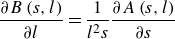 \begin{equation} \frac {\partial B\left (s,l\right )}{\partial l}=\frac {1}{l^{2}s}\frac {\partial A\left (s,l\right )}{\partial s} \end{equation}
and performing the integral by parts with respect to
 $s$
,
 $F (r,t )$
can be simplified as
 \begin{equation} F\left (r,t\right )=-\frac {\epsilon _{\infty }(t)}{r^{3}}\frac {\int _{0}^{\infty }{\rm d}l\ l\left [rA\left (r,l\right )-\int _{0}^{r}ds\ A\left (s,l\right )\right ]f\left (l,t\right )}{\int _{0}^{\infty }{\rm d}l \left (k_{f}l\right )^{2}j_{2}\left (k_{f}l\right )f\left (l,t\right )} \end{equation}
with
 \begin{align} rA\left (r,l\right )-\int _{0}^{r}{\rm d}s\ A\left (s,l\right )=rl\left [2j_{0}\left (k_{f}r\right )j_{0}\left (k_{f}l\right )-j_{0}\left (k_{f}\left (r+l\right )\right )-j_{0}\left (k_{f}\left (r-l\right )\right )\right ], \\[-24pt] \nonumber \end{align}
where we assumed
 $f (r,t )\to 0$
as
 $r\to \infty$
.
The third-order longitudinal velocity structure function is then written as
 \begin{align} S_{3}^{L}\left (r,t\right )&=6\nu \frac {\partial S_{2}^{L}\left (r,t\right )}{\partial r}-\frac {4}{5}\left (\epsilon (t)-\epsilon _{\infty }(t)\right )r-\frac {3}{r^{4}}\int _{0}^{r}{\rm d}s\ s^{4}\frac {\partial S_{2}^{L}\left (s,t\right )}{\partial t}\notag\\&\quad -\epsilon _{\infty }(t)\frac {\int _{0}^{\infty }{\rm d}l\ lg_{N}\left (k_{f}l,k_{f}r\right )f\left (l,t\right )}{\int _{0}^{\infty }{\rm d}l\ g_{D}\left (k_{f}l\right )f\left (l,t\right )}, \end{align}
with
 \begin{align} g_{N}\left (x,y\right )=\frac {6}{y^{4}}&\left [x^{3}\left \{\textrm {Si}\left (x-y\right )-\textrm {Si}\left (x+y\right )\right \}+2x^{2}\sin x\sin y+2x^{2}y^{2}j_{1}\left (x\right )j_{1}\left (y\right )\right ], \\[-12pt] \nonumber \end{align}
 \begin{align} &\qquad\qquad g_{D}\left (x\right )=-x^{2}j_{2}\left (x\right ), \\[16pt] \nonumber \end{align}
where
 $\textrm {Si} (x )$
is the sine integral. Equation (A9) is an exact representation of the third-order longitudinal velocity structure function for deterministic forcing of the form (2.3) with
 $\boldsymbol {u}^{f}$
and
 $g (\boldsymbol {x} )=4\pi k_{f}^{3}j_{1} (k_{f}|\boldsymbol {x}| )/(k_{f}|\boldsymbol {x}|)$
. Assuming that the turbulence is statistically stationary and neglecting the viscous effect, using the Taylor expansion
 $g_{N} (x,y\to 0 )=-4xj_{2} (x )/5y+\mathcal {O} (y^{3} )$
yields the third-order longitudinal velocity structure function as follows:
 \begin{equation} S_{3}^{L}\left (r\to 0\right )=-\frac {4}{5}\epsilon r+\mathcal {O}\big (r^{3}\big ), \end{equation}
where the above equation is known as Kolmogorov’s four-fifths law (Kolmogorov Reference Kolmogorov1941a ).
Next, we consider the normalised energy dissipation rate for the present deterministic forcing. Using the relations
 $S_{2}^{L} (r,t )=2u^{2}(t) [1-f (r,t ) ]$
and
 $S_{3}^{L} (r,t )=6u^{3}(t)K(r,t)$
(Davidson Reference Davidson2015), the KHE can also be written as (2.1). Integrating (2.1) with respect to
 $r$
from 0 to
 $\infty$
, we have
 \begin{align} \frac {{\rm d}u^{2}\left (t\right )L\left (t\right )}{{\rm d}t}&=u^{3}\left (t\right )\int _{0}^{\infty }{\rm d}r \frac {1}{r^{4}}\frac {\partial }{\partial r}\left [r^{4}K\left (r,t\right )\right ]+2\nu u^{2}\left (t\right )\int _{0}^{\infty }{\rm d}r\ \frac {1}{r^{4}}\frac {\partial }{\partial r}\left [r^{4}\frac {\partial f\left (r,t\right )}{\partial r}\right ]\notag\\ &\quad -\frac {\epsilon _{\infty }(t)u^{2}\left (t\right )}{2K_{f}\left (t\right )}\int _{0}^{\infty }{\rm d}l\ \left [-2+2\cos \left (k_{f}l\right )+k_{f}l\sin \left (k_{f}l\right )\right ]f\left (l,t\right ), \end{align}
where
 $\int _{0}^{\infty }{\rm d}l\ [- (k_{f}l )^{2}j_{2} (k_{f}l ) ]f (l,t )=-\pi K_{f} (t )/ (k_{f}u^2 (t ) )$
was used. By defining
 $L_{f} (t )=3\pi / (4K_{f} (t ) )\int _{0}^{k_{f}}{\rm d}k\ E (k,t )/k$
, the above equation becomes
 \begin{align} \frac {{\rm d}u^{2}(t)L(t)}{{\rm d}t}&=u^{3}(t)\int _{0}^{\infty }{\rm d}r \frac {1}{r^{4}}\frac {\partial }{\partial r}\left [r^{4}K\left (r,t\right )\right ]+2\nu u^{2}(t)\int _{0}^{\infty }{\rm d}r\ \frac {1}{r^{4}}\frac {\partial }{\partial r}\left [r^{4}\frac {\partial f\left (r,t\right )}{\partial r}\right ]\notag\\ &\quad+\frac {2}{3}\epsilon _{\infty }(t)L_{f}(t), \end{align}
where
 $\int _{0}^{\infty }{\rm d}l\ [\cos (k_{f}l )+k_{f}l/2\sin (k_{f}l ) ]f (l,t )=\pi /(2u^2(t))\int _{k_{f}}^{\infty }{\rm d}k\ E (k,t )/k$
was used. Using
 ${\rm d}u^{2} (t )/{\rm d}t=2/3 (-\epsilon (t )+\epsilon _{\infty }(t) )$
and dividing the above equation by
 $u^3 (t )$
,
 $C_{\epsilon } (t )$
can be written as (2.7).
A.1.1. Derivation from the Lin equation
It may be easier to derive the forced KHE and
 $C_{\epsilon }(t)$
from the Lin equation. The Lin equation for the current deterministic forcing is given as
 \begin{equation} \left [\frac {\partial }{\partial t}+2\nu k^{2}\right ]E\left (k,t\right )=T\left (k,t\right )+\frac {\epsilon _{\infty }(t)}{K_{f}\left (t\right )}E\left (k,t\right )\left [H\left (k\right )-H\left (k-k_{f}\right )\right ], \end{equation}
where
 $T (k,t )$
is the energy transfer function and it can be defined in terms of the energy flux as
 $T (k,t )=-\partial _{k}\Pi (k,t )$
or
 $\Pi (k,t )=-\int _{0}^{k}{\rm d}p\ T (p,t )=\int _{k}^{\infty }{\rm d}p\ T (p,t )$
, where
 $\Pi (0,t )=\Pi (\infty ,0 )=0$
holds.
For homogeneous isotropic turbulence, the following relationships apply (Davidson Reference Davidson2015):
 \begin{align} &S_{2}^{L}\left (r,t\right )=4\int _{0}^{\infty }{\rm d}k\ E\left (k,t\right )\left [\frac {1}{3}-\frac {j_{1}\left (kr\right )}{kr}\right ], \end{align}
 \begin{align} &\quad S_{3}^{L}\left (r,t\right )=12r\int _{0}^{\infty }{\rm d}k\ T\left (k,t\right )\frac {j_{2}\left (kr\right )}{\left (kr\right )^{2}}, \end{align}
and using the orthogonality of the spherical Bessel function gives the inverse relations
 \begin{align} E\left (k,t\right )=\frac {1}{2\pi }\int _{0}^{\infty }{\rm d}r\ \left [2u^{2}-S_{2}^{L}\left (r,t\right )\right ]\left (kr\right )^{3}j_{1}\left (kr\right ), \end{align}
 \begin{align} T\left (k,t\right )=\frac {k^{2}}{6\pi }\int _{0}^{\infty }{\rm d}r\ j_{0}\left (kr\right )\frac {\partial }{\partial r}\left [\frac {1}{r}\frac {\partial }{\partial r}\left (r^{4}S_{3}^{L}\left (r,t\right )\right )\right ]. \end{align}
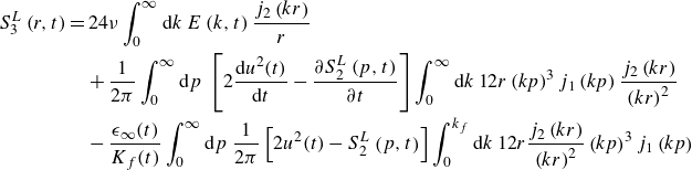
Integrating (A14) multiplied by
 $12rj_{2} (kr )/ (kr )^{2}$
and substituting (A16a
) for
 $E (k,t )$
gives
 \begin{align} S_{3}^{L}\left (r,t\right )&=24\nu \int _{0}^{\infty }{\rm d}k\ E\left (k,t\right )\frac {j_{2}\left (kr\right )}{r} \notag\\ &\quad +\frac {1}{2\pi }\int _{0}^{\infty }{\rm d}p\ \left [2\frac {{\rm d}u^2(t)}{{\rm d}t}-\frac {\partial S_{2}^{L}\left (p,t\right )}{\partial t}\right ]\int _{0}^{\infty }{\rm d}k\ 12r\left (kp\right )^{3}j_{1}\left (kp\right )\frac {j_{2}\left (kr\right )}{\left (kr\right )^{2}}\notag\\ &\quad -\frac {\epsilon _{\infty }(t)}{K_{f}(t)}\int _{0}^{\infty }{\rm d}p\ \frac {1}{2\pi }\left [2u^2(t)-S_{2}^{L}\left (p,t\right )\right ]\int _{0}^{k_{f}}{\rm d}k\ 12r\frac {j_{2}\left (kr\right )}{\left (kr\right )^{2}}\left (kp\right )^{3}j_{1}\left (kp\right ) \end{align}
where using
 $\partial _{r}S_{2}^{L} (r,t )=4\int _{0}^{\infty }{\rm d}k\ E (k,t )j_{2} (kr )/r$
gives the first term in (A9) and using
 $6r/\pi \int _{0}^{\infty }{\rm d}k\ (kp )^{3}j_{1} (kp )j_{2} (kr )/ (kr )^{2}=3p^4/r^4$
for
 $p\lt r$
(zero for
 $p\gt r$
) gives the second and third terms in (A9). Similarly, some integral formulae give the last term in (A9) (Abramowitz & Stegun Reference Abramowitz and Stegun1964; Gradshteyn & Ryzhik Reference Gradshteyn and Ryzhik2014).
Next, we consider
 $C_{\epsilon }(t)$
as in Appendix A.1. Integrating (A14) multiplied by
 $1/k$
and using
 $\int _{0}^{\infty }{\rm d}k\ E (k,t )/k=2u^2(t)L(t)/\pi$
yields
 \begin{equation} \frac {3}{2}\frac {{\rm d} u^{2}(t)L(t)}{{\rm d}t}=\frac {3\pi }{4}\!\int _{0}^{\infty }\!{\rm d}k\ \frac {T\left (k,t\right )}{k}-\frac {3\pi \nu }{2}\!\int _{0}^{\infty }\!{\rm d}k\ kE\left (k,t\right )+\frac {3\pi }{4}\frac {\epsilon _{\infty }(t)}{K_{f}(t)}\!\int _{0}^{k_{f}}\!{\rm d}k\ \frac {E\left (k,t\right )}{k}. \end{equation}
Dividing the above equation by
 $u^{3}(t)$
and rearranging the resulting equation,
 $C_{\epsilon }(t)$
can be written as
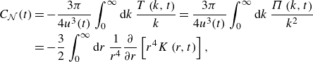
 \begin{equation} C_{\epsilon }(t)=\alpha _{f}\left [C_{\mathcal {N}}(t)+\frac {C_{\mathcal {D}}(t)}{Re_{L}(t)}+\frac {3}{2}\frac {1}{u(t)}\frac {{\rm d}L(t)}{{\rm d}t}\right ], \end{equation}
where
 \begin{align} C_{\mathcal {N}}(t)&=-\frac {3\pi }{4u^{3}(t)}\int _{0}^{\infty }{\rm d}k\ \frac {T\left (k,t\right )}{k}=\frac {3\pi }{4u^3(t)}\int _{0}^{\infty }{\rm d}k\ \frac {\Pi \left (k,t\right )}{k^2}\notag\\&=-\frac {3}{2}\int _{0}^{\infty }{\rm d}r\ \frac {1}{r^{4}}\frac {\partial }{\partial r}\left [r^{4}K\left (r,t\right )\right ], \end{align}
 \begin{equation} C_{\mathcal {D}}(t)=\frac {3\pi L(t)}{2u^{2}(t)}\int _{0}^{\infty }{\rm d}k\ kE\left (k,t\right )=-3L(t)\int _{0}^{\infty }{\rm d}r\ \frac {1}{r^{4}}\frac {\partial }{\partial r}\left [r^{4}\frac {\partial f\left (r,t\right )}{\partial r}\right ], \end{equation}
where the two equalities can be derived from the isotropic relations (A15a )–(A16b ).
A.2 Stochastic forcing
Next, we consider the stochastic force introduced in § 2.2. To take the functional derivative, we make the formal functional consequence from the Fourier transformed Navier–Stokes equation:
 \begin{align} \hat {u}_{i}\left (\boldsymbol {k},t\right )&=\hat {u}_{i}\left (\boldsymbol {k},t_{0}\right )+M_{ijk}\left (\boldsymbol {k}\right )\int _{t_{0}}^{t}{\rm d}s\ \int _{\boldsymbol {k}=\boldsymbol {p}+\boldsymbol {q}}{\rm d}\boldsymbol {p}\ \hat {u}_{j}\left (\boldsymbol {p},s\right )\hat {u}_{k}\left (\boldsymbol {q},s\right )\notag\\&\quad -\nu k^{2}\int _{t_{0}}^{t}{\rm d}s\ \hat {u}_{i}\left (\boldsymbol {k},s\right )+\int _{t_{0}}^{t}{\rm d}s\ \hat {f}_{i}\left (\boldsymbol {k},s\right ), \end{align}
where
 $M_{ijk} (\boldsymbol {k} )=-\imath /2 [k_{j}P_{ik} (\boldsymbol {k} )+k_{k}P_{ij} (\boldsymbol {k} ) ]$
is the symmetric tensor with respect to
 $j$
and
 $k$
. The functional derivative is then given by
 \begin{align} \frac {\delta \hat {u}_{i}\left (\boldsymbol {k},t\right )}{\delta \hat {f}_{j}\left (\boldsymbol {p},s\right )}&=2M_{i\alpha \beta }\left (\boldsymbol {k}\right )\!\int _{s}^{t}\!{\rm d}s' \int _{\boldsymbol {k}=\boldsymbol {p}+\boldsymbol {q}}\!{\rm d}\boldsymbol {p}\ \hat {u}_{\alpha }\left (\boldsymbol {p},s'\right )\frac {\delta \hat {u}_{\beta }\left (\boldsymbol {q},s'\right )}{\delta \hat {f}_{j}\left (\boldsymbol {p},s\right )}-\nu k^{2}\!\int _{s}^{t}\!{\rm d}s'\ \frac {\delta \hat {u}_{i}\left (\boldsymbol {k},s'\right )}{\delta \hat {f}_{j}\left (\boldsymbol {p},s\right )}\notag\\ &\quad +\delta _{ij}\delta \left (\boldsymbol {k}-\boldsymbol {p}\right )H\left (t-s\right )H\left (s-t_{0}\right ), \end{align}
where the lower limits of the integrals in the first two summands are modified according to the causality principle. Substituting
 $\delta \hat {\boldsymbol {u}}/\delta \,\hat {\boldsymbol {\!f}}$
into the Furutsu–Novikov–Donsker theorem (2.10) and using the properties of the delta function, we get
 \begin{equation} \left \langle \hat {f}_{i}\left (\boldsymbol {k},t\right )\hat {u}_{j}\left (\boldsymbol {p},s\right )\right \rangle =\begin{cases} \frac {F\left (k\right )}{8\pi k^{2}}P_{ij}\left (\boldsymbol {k}\right )\delta \left (\boldsymbol {k}+\boldsymbol {p}\right ) & (t=s), \\ 0 & (t\gt s), \end{cases} \end{equation}
where
 $\int _{t_{0}}^{t}{\rm d}s\ \delta (t-s )=1/2$
and
 $\delta (t-s )\int _{s}^{t}{\rm d}s' =0$
were used in the derivation. Assuming the isotropy and using (A22) and (A23), the velocity–force correlation can be written as
 \begin{equation} \left \langle \boldsymbol {f}\cdot \boldsymbol {u}'\right \rangle =\int _{0}^{\infty }{\rm d}k\ j_{0}\left (kr\right )F\left (k\right ), \end{equation}
and the following results:
 \begin{equation} F\left (r\right )=\frac {1}{r^{3}}\int _{0}^{r}{\rm d}s\ s^{2}\left [\left \langle \boldsymbol {f}\cdot \boldsymbol {u}'\right \rangle +\left \langle \boldsymbol {f}'\cdot \boldsymbol {u}\right \rangle \right ]=2\int _{0}^{\infty }{\rm d}k\ \frac {j_{1}\left (kr\right )}{kr}F\left (k\right ). \end{equation}
The third-order longitudinal velocity structure function is then written as
 \begin{align} S_{3}^{L}\left (r,t\right )&=6\nu \frac {\partial S_{2}^{L}\left (r,t\right )}{\partial r}-\frac {4}{5}\left (\epsilon (t)-\epsilon _{\infty }\right )-\frac {3}{r^{4}}\int _{0}^{r}ds\ s^{4}\frac {\partial S_{2}^{L}\left (s,t\right )}{\partial t}\notag\\&\quad -12\int _{0}^{\infty }dk\ \frac {F\left (k\right )}{k}\frac {j_{2}\left (kr\right )}{kr}, \end{align}
where the above representation was also derived by Fukayama et al. (Reference Fukayama, Oyamada, Nakano, Gotoh and Yamamoto2000). Assuming the statistically stationary state of the turbulence and neglecting the viscous term, the Taylor expansion yields
 \begin{equation} S_{3}^{L}\left (r\to 0\right )=-\frac {4}{5}\epsilon r+\frac {2}{35}r^{3}\int _{0}^{\infty }{\rm d}k\ k^{2}F\left (k\right )+\mathcal {O}\left (r^{5}\right ), \end{equation}
where a first term on the right-hand side represents Kolmogorov’s four-fifths law. If
 $F(k)$
is given by the steeper power-law function over the wide wavenumber range or by the compact form at the low wavenumber, the first term is a leading term, and the higher-order terms do not affect the power-law scaling of
 $S_{3}^{L}(r)$
in the inertial subrange.
Integrating (2.1) using (2.12) with respect to
 $r$
from 0 to
 $\infty$
,
 $C_{\epsilon }(t)$
is the same as (2.7), but
 $L_{f}(t)$
in
 $\alpha _{f}(t)$
is the forcing integral length scale defined by (2.13)
A.3. General forcing
Finally, we discuss
 $C_{\epsilon }(t)$
without considering the concrete form of the forcing. The forcing obeying the Ornstein–Uhlenbeck process (Eswaran & Pope Reference Eswaran and Pope1988) and the Taylor–Green forcing (Goto & Vassilicos Reference Goto and Vassilicos2015, Reference Goto and Vassilicos2016) are considered as the examples. Our starting point is the Fourier transformed Navier–Stokes equation:
 \begin{equation} \frac {\partial \hat {u}_{i}\left (\boldsymbol {k},t\right )}{\partial t}=M_{ijk}\left (\boldsymbol {k}\right )\int _{\boldsymbol {k}=\boldsymbol {p}+\boldsymbol {q}}{\rm d}\boldsymbol {p}\ \hat {u}_{j}\left (\boldsymbol {p},t\right )\hat {u}_{k}\left (\boldsymbol {q},t\right )-\nu k^{2}\hat {u}_{i}\left (\boldsymbol {k},t\right )+\hat {f}_{i}\left (\boldsymbol {k},t\right ). \end{equation}
Multiplying
 $\hat {u}_{i}^{*} (\boldsymbol {k},t )$
and adding the complex conjugate of the resulting equation and taking the proper integral over the angle variables, we obtain the Lin equation
 \begin{equation} \frac {\partial E\left (k,t\right )}{\partial t}=T\left (k,t\right )-2\nu k^{2}E\left (k,t\right )+F\left (k,t\right ), \end{equation}
where
 \begin{align} &\quad E\left (k,t\right )=\oint {\rm d}S\ \hat {\boldsymbol {u}}\left (\boldsymbol {k},t\right )\cdot \hat {\boldsymbol {u}}^{*}\left (\boldsymbol {k},t\right ), \end{align}
 \begin{align} &T\left (k,t\right )=\oint {\rm d}S\ \hat {\boldsymbol {N}}\left (\boldsymbol {k},t\right )\cdot \hat {\boldsymbol {u}}^{*}\left (\boldsymbol {k},t\right )+\textrm {c.c.}, \end{align}
 \begin{align} &F\left (k,t\right )=\oint {\rm d}S\ \,\hat {\boldsymbol {\!f}}\left (\boldsymbol {k},t\right )\cdot \hat {\boldsymbol {u}}^{*}\left (\boldsymbol {k},t\right )+\textrm {c.c.}, \end{align}
where
 $\hat {\boldsymbol {N}} (\boldsymbol {k},t )$
is the nonlinear term in Navier–Stokes equation,
 $\textrm {c.c.}$
represents the complex conjugate, and
 $\oint {\rm d}S=1/2\int _{0}^{\pi }{\rm d}\theta _{k}\ \sin \theta _{k}\int _{0}^{2\pi }{\rm d}\phi _{k}$
with polar angle
 $\theta _{k}$
and azimuthal angle
 $\phi _{k}$
. As in § A.1.1, multiplying
 $1/k$
by the Lin equation and integrating with respect to
 $k$
from 0 to
 $\infty$
, and rearranging the resulting equation, we have the same expression in § A.1, but
 $L_{f}(t)$
has the same definition in Appendix A.2.
A.4. Mean velocity gradient as forcing
The non-equilibrium dissipation law
 $C_{\epsilon }\sim \sqrt {Re_{0}}/Re_{\lambda }$
has been observed in various complex turbulent flows (Vassilicos Reference Vassilicos2015). It is considered that the phenomenology of
 $C_{\epsilon }$
in complex turbulent flows may be different from that in isotropic turbulence and, therefore, it is important to revisit
 $C_{\epsilon }$
in strain- and shear-driven turbulence as such turbulent flows are encountered in the real world.
We consider homogeneous turbulence distorted by a space-uniform mean velocity gradient
 $\lambda _{ij} (t )=\partial U_{i}/\partial x_{j}$
. The spectral tensor equation is written as (Townsend Reference Townsend1976; Mons, Cambon & Sagaut Reference Mons, Cambon and Sagaut2016; Sagaut & Cambon Reference Sagaut and Cambon2018)
 \begin{equation} \left (\frac {\partial }{\partial t}+2\nu k^{2}-\lambda _{ln}(t)k_{l}\frac {\partial }{\partial k_{n}}\right )\Phi _{ii}\left (\boldsymbol {k},t\right )+2\lambda _{in}\left (t\right )\Phi _{ni}\left (\boldsymbol {k},t\right )=T_{ii}\left (\boldsymbol {k},t\right ), \end{equation}
where
 $\Phi _{ij} (\boldsymbol {k},t )\delta (\boldsymbol {k}-\boldsymbol {p} )=\langle \hat {u}_{i}^{*} (\boldsymbol {p},t )\hat {u}_{j} (\boldsymbol {k},t )\rangle$
and
 $T_{ij} (\boldsymbol {k},t )$
is the nonlinear spectral tensor. Without loss of generality, the anisotropy of the theory should necessarily be taken into account for turbulence in the presence of the mean velocity gradient. Following Cambon & Rubinstein (Reference Cambon and Rubinstein2006), we use the representation of a spherically averaged descriptor for
 $\Phi _{ij} (\boldsymbol {k},t )$
. It is written as
 \begin{align} \Phi _{ij}\left (\boldsymbol {k},t\right )&=\frac {E\left (k,t\right )}{4\pi k^{2}}\left [1-15H_{\alpha \beta }^{(dir)}\left (k,t\right )\frac {k_{\alpha }k_{\beta }}{k^{2}}\right ]P_{ij}\left (\boldsymbol {k}\right )\notag\\ &\quad +5\frac {E\left (k,t\right )}{4\pi k^{2}}\left [P_{i\alpha }\left (\boldsymbol {k}\right )P_{j\beta }\left (\boldsymbol {k}\right )+\frac {1}{2}P_{ij}\left (\boldsymbol {k}\right )\frac {k_{\alpha }k_{\beta }}{k^{2}}\right ]H_{\alpha \beta }^{(pol)}\left (k,t\right ), \end{align}
where
 $H_{ij}^{(dir)} (k,t )$
and
 $H_{ij}^{(pol)} (k,t )$
are directional and polarisation anisotropies. The tensor
 $H_{ij}^{(\alpha )}$
is symmetric and trace-free (Cambon & Rubinstein Reference Cambon and Rubinstein2006; Mons et al. Reference Mons, Cambon and Sagaut2016). Substituting (A32) into (A31) and integrating the resulting equation over the angle variables, we have the Lin equation
 \begin{equation} \frac {\partial E\left (k,t\right )}{\partial t}=T\left (k,t\right )-2\nu k^{2}E\left (k,t\right )+F\left (k,t\right ), \end{equation}
where the forcing spectrum in (A33) results from the mean velocity gradient and can be written as (Mons et al. Reference Mons, Cambon and Sagaut2016)
 \begin{align} F\left (k,t\right )&=-2S_{lm}\left (t\right )\frac {\partial }{\partial k}\left [kE\left (k,t\right )H_{lm}^{(dir)}\left (k,t\right )\right ]\notag\\&\quad -2E\left (k,t\right )S_{lm}\left (t\right )\left [H_{lm}^{(dir)}\left (k,t\right )+H_{lm}^{(pol)}\left (k,t\right )\right ], \end{align}
where
 $S_{ij} (t )= [\lambda _{ij} (t )+\lambda _{ji} (t ) ]/2$
. We used the formulae
 $\oint {\rm d}S\ k_{i}k_{j}k^{-2}=2\pi k^{2}/3\delta _{ij}$
and
 $\oint dS\ k_{i}k_{j}k_{l}k_{m}k^{-4}=2\pi k^{2}/15 (\delta _{ij}\delta _{lm}+\delta _{il}\delta _{jm}+\delta _{im}\delta _{jl} )$
in the derivation.
For the present forcing,
 $\alpha _{f}(t)$
is given by
 \begin{equation} \alpha _{f}(t)=\left [1+\frac {3S_{lm}(t)u^2(t)}{\epsilon (t)}\left (b_{lm}^{(dir)}(t)+b_{lm}^{(pol)}(t)\right )\left (1-\frac {L_{f}(t)}{L(t)}\right )\right ]^{-1}, \end{equation}
where
 $b_{lm}^{(\alpha )}(t)=\int _{0}^{\infty }{\rm d}k\ E (k,t )H_{lm}^{(\alpha )} (k,t )/(3u^2(t)/2)$
and
 $L_{f}(t)$
is defined as
 \begin{equation} L_{f}(t)=\frac {3\pi }{4}\frac {S_{\alpha \beta }(t)\int _{0}^{\infty }{\rm d}k\ k^{-1}E\left (k,t\right )\left [2H_{\alpha \beta }^{(dir)}\left (k,t\right )+H_{\alpha \beta }^{(pol)}\left (k,t\right )\right ]}{S_{\gamma \delta }(t)\int _{0}^{\infty }{\rm d}k\ E\left (k,t\right )\left [H_{\gamma \delta }^{(dir)}\left (k,t\right )+H_{\gamma \delta }^{(pol)}\left (k,t\right )\right ]}. \end{equation}
We simplify (A35) as follows:
 \begin{equation} \alpha _{f}(t)=\left [1+\frac {3S(t)u^2(t)}{2\epsilon (t)}\right ]^{-1}=\frac {1}{1+\tilde {S}(t)}, \end{equation}
where
 $\tilde {S}(t)=3Su^2(t)/(2\epsilon (t))$
is a non-dimensional time scale ratio (Ayyalasomayajula & Warhaft Reference Ayyalasomayajula and Warhaft2006) and
 $S(t)$
may be regarded as the representative eigenvalue of
 $S_{lm}(t)$
. It was experimentally shown that
 $\tilde {S}\propto Re_{\lambda }$
for axisymmetric strain turbulent flow (Ayyalasomayajula & Warhaft Reference Ayyalasomayajula and Warhaft2006) and for shear turbulent flow (Ferchichi & Tavoularis Reference Ferchichi and Tavoularis2000). If the rapid distortion cannot be ignored, it is expected
 $C_{\epsilon }(t)\propto \alpha _{f}(t)=1/ [1+\gamma Re_{\lambda }(t) ]$
, where
 $\gamma$
is a constant and may be related to the inverse of
 $\sqrt {Re_{0}}$
, and we have omitted the contribution of
 $u^{-1}(t)dL(t)/dt$
to
 $C_{\epsilon }(t)$
. Hence,
 $C_{\epsilon }(t)\propto Re_{\lambda }^{-1}(t)$
when
 $1\ll \gamma Re_{\lambda }(t)$
and
 $C_{\epsilon }(t)\geqslant C_{\mathcal {N}}(t)$
when
 $1\gg \gamma Re_{\lambda }(t)$
. However, it is expected that
 $C_{\mathcal {N}}(t)\approx \textrm {const.}$
holds even for
 $1\ll \gamma Re_{\lambda }$
.
To justify our phenomenological consideration, we consider the skewness of velocity gradient tensor
 $S_{\partial u/\partial x}=\langle (\partial u_{1}/\partial x_{1} )^{3}\rangle /\langle (\partial u_{1}/\partial x_{1} )^{2}\rangle ^{3/2}$
. Assuming isotropy, the skewness of velocity gradient tensor is written as (Lesieur Reference Lesieur2008)
 \begin{equation} S_{\partial u/\partial x}(t)=-\frac {15\sqrt {15}}{7\sqrt {2}}\frac {\int _{0}^{\infty }{\rm d}k\ k^{2}T\left (k,t\right )}{\left [\int _{0}^{\infty }{\rm d}k\ k^{2}E\left (k,t\right )\right ]^{\frac {3}{2}}}, \end{equation}
and the Lin equation (A33) with the use of (A34) yields
 \begin{equation} S_{\partial u/\partial x}(t)\approx -\frac {15\sqrt {30}\nu }{7}\frac {\int _{0}^{\infty }{\rm d}k\ k^{4}E\left (k,t\right )}{\left [\int _{0}^{\infty }{\rm d}k\ k^{2}E\left (k,t\right )\right ]^{\frac {3}{2}}}+\frac {15\sqrt {15}}{7\sqrt {2}}\frac {S_{lm}(t)\left (d_{lm}^{(dir)}(t)-d_{lm}^{(pol)}(t)\right )}{\sqrt {\int _{0}^{\infty }{\rm d}k\ k^{2}E\left (k,t\right )}}, \end{equation}
where
 $d_{ij}^{(\alpha )}(t)=4\nu \int _{0}^{\infty }{\rm d}k\ k^{2}E (k,t )H_{ij}^{(\alpha )}(k,t)/\epsilon$
,
 $\left .k^3 E (k,t )H_{lm}^{(dir)}(k,t)\right |_{k=\infty }=0$
was used and we omitted the time derivative term. The second term works out to be positive because it represents the production of dissipation and is written as
 $2\nu \int _{0}^{\infty }{\rm d}k\ k^{2}F (k,t )=S_{lm}(t)\epsilon (t) (d_{lm}^{(dir)}(t)-d_{lm}^{(pol)}(t) )=C_{\epsilon 1}\mathcal {P}(t)\epsilon (t)/(3u^2(t)/2)=-C_{\epsilon 1}\lambda _{lm}(t)\langle u_{l}u_{m}\rangle (t)\epsilon (t)/(3u^2(t)/2)$
in the
 $K$
–
 $\epsilon$
model (Wilcox Reference Wilcox1998; Piquet Reference Piquet2001; Durbin & Reif Reference Durbin and Reif2011; Mons et al. Reference Mons, Cambon and Sagaut2016), where
 $C_{\epsilon 1}$
is a positive constant and
 $\mathcal {P}(t)$
is a production term in the transport equation of turbulent kinetic energy. As in the previous discussion, the second term in (A39) may be simplified as
 $S(t)/\sqrt {\langle \boldsymbol {\omega }^{2}\rangle (t)}$
. Taking the grid turbulence as an example, the axial strain at the grid-element centreline and the shear at the lee of the grid-element are candidates for
 $S(t)$
, and
 $S(t)$
is the monotonically decreasing function from the upstream to downstream. According to the experiments (Hearst & Lavoie Reference Hearst and Lavoie2014), the energy spectra obey the Kolmogorov scaling, and it is then assumed that the first term in (A39) is nearly constant during the decay. However, the contribution of the second term gradually vanishes as the turbulence evolves, and hence, the magnitude of
 $S_{\partial u/\partial x}$
gradually increases as the turbulence evolves. Thus, our phenomenological theory provides a reasonable explanation for the relationship between non-equilibrium properties and residual strain (Hearst & Lavoie Reference Hearst and Lavoie2015). However, our results suggest that in contrast to their conclusion, the importance of large-scale properties on the small scales is negligible, and the Kolmogorov theory is not violated.
Note that the present explanation is that the origin of
 $C_{\epsilon }\propto Re_{\lambda }^{-1}$
has its origin in
 $\tilde {S}(t)$
, and it is conjectured that whether
 $u^{-1}(t){\rm d}L(t)/{\rm d}t$
or
 $\tilde {S}(t)$
contributes to
 $C_{\epsilon }\propto Re_{\lambda }^{-1}$
in a dominant manner depends on the flow field. Nevertheless, the present explanation is based on the phenomenology and not experimental and numerical evidence. Thus, further investigations will be conducted in future studies.
Appendix B. Numerical method
The incompressible Navier–Stokes equations were solved by the pseudo-spectral method under periodic boundary conditions with the period of
 $2\pi$
in each of the three Cartesian coordinate directions. The phase-shift method was used for dealiasing, in which the maximum wavenumber of the retained Fourier modes was approximately
 $\sqrt {2}N/3$
, where
 $N^{3}$
was the number of grid points. We used the fourth-order Runge–Kutta scheme for the time advance of nonlinear and viscous terms irrespective of forcing method. The numerical code was parallelised using the message-passing interface library and OpenMP (Kitamura Reference Kitamura2020).
The temporal statistical quantities in a snapshot are calculated from
 \begin{align} &\quad u^2(t)=\frac {1}{3}\sum _{\boldsymbol {k}}\hat {\boldsymbol {u}}\left (\boldsymbol {k},t\right )\cdot \hat {\boldsymbol {u}}^{*}\left (\boldsymbol {k},t\right ), \end{align}
 \begin{align} &\quad \epsilon (t)=\nu \sum _{\boldsymbol {k}}k^{2}\hat {\boldsymbol {u}}\left (\boldsymbol {k},t\right )\cdot \hat {\boldsymbol {u}}^{*}\left (\boldsymbol {k},t\right ), \end{align}
 \begin{align} &L(t)=\frac {\pi }{4u^2(t)}\sum _{\boldsymbol {k}}\frac {\hat {\boldsymbol {u}}\left (\boldsymbol {k},t\right )\cdot \hat {\boldsymbol {u}}^{*}\left (\boldsymbol {k},t\right )}{k}, \end{align}
where
 $\sum _{\boldsymbol {k}}$
denotes the discrete summation in the wavenumber space. The Taylor microscale is defined as
 $\lambda (t)=\sqrt {15\nu u^2(t)/\epsilon (t)}$
and the Kolmogorov length scale as
 $\eta (t)= (\nu ^{3}/\epsilon (t) )^{1/4}$
. The Reynolds number based on the Taylor microscale is defined as
 $Re_{\lambda }(t)=u(t)\lambda (t)/\nu$
. The normalised energy dissipation rate is defined as
 $C_{\epsilon }(t)=\epsilon (t) L(t)/u^3(t)$
.
Here,
 $C_{\mathcal {N}}(t)$
,
 $C_{\mathcal {D}}(t)/Re_{L}(t)$
and
 $u^{-1}(t){\rm d}L(t)/{\rm d}t$
are calculated from
 \begin{align} &\qquad C_{\mathcal {N}}(t)=-\frac {3\pi }{8u^3(t)}\sum _{\boldsymbol {k}}\frac {1}{k}\left [ \hat {\boldsymbol {N}}\left (\boldsymbol {k},t\right )\cdot \hat {\boldsymbol {u}}^{*}\left (\boldsymbol {k},t\right )+\textrm {c.c.}\right ], \end{align}
 \begin{align} &\qquad\qquad \frac {C_{\mathcal {D}}(t)}{Re_{L}(t)}=\frac {3\pi \nu }{4u^3(t)}\sum _{\boldsymbol {k}}k \hat {\boldsymbol {u}}\left (\boldsymbol {k},t\right )\cdot \hat {\boldsymbol {u}}^{*}\left (\boldsymbol {k},t\right ), \end{align}
 \begin{align} &\frac {1}{u(t)}\frac {dL(t)}{dt}=\frac {\pi }{2u^3(t)}\sum _{\boldsymbol {k}}\frac {d}{dt}\frac {\hat {\boldsymbol {u}}\left (\boldsymbol {k},t\right )\cdot \hat {\boldsymbol {u}}^{*}\left (\boldsymbol {k},t\right )}{k}+\frac {2}{3}\frac {\epsilon (t)L(t)}{u^{3}(t)}, \end{align}
and
 $\alpha _{f}(t)$
is calculated from
 $\alpha _{f}(t)= [1-\epsilon _{\infty }(t)/\epsilon (t)+\epsilon _{\infty }(t)L_{f}(t)/(\epsilon (t) L(t)) ]^{-1}$
.
Equation (2.7) is an exact relation derived from the Kármán–Howarth equation, however, the evaluation of statistical quantities using a snapshot may be insufficient from a statistical point of view. We define the statistical quantities to be consistent with the theoretical argument. The results presented in figure 2 for decaying turbulence are calculated from
 \begin{align} &\,\,u^2(t)=\frac {1}{N}\sum _{n=1}^{N}\frac {1}{3}\sum _{\boldsymbol {k}}\hat {\boldsymbol {u}}^{(n)}\left (\boldsymbol {k},t\right )\cdot \hat {\boldsymbol {u}}^{*(n)}\left (\boldsymbol {k},t\right ), \end{align}
 \begin{align} &\,\,\epsilon (t)=\frac {1}{N}\sum _{n=1}^{N}\nu \sum _{\boldsymbol {k}}k^{2}\hat {\boldsymbol {u}}^{(n)}\left (\boldsymbol {k},t\right )\cdot \hat {\boldsymbol {u}}^{*(n)}\left (\boldsymbol {k},t\right ), \end{align}
 \begin{align} &L(t)=\frac {\pi }{4u^2(t)}\frac {1}{N}\sum _{n=1}^{N}\sum _{\boldsymbol {k}}\frac {\hat {\boldsymbol {u}}^{(n)}\left (\boldsymbol {k},t\right )\cdot \hat {\boldsymbol {u}}^{*(n)}\left (\boldsymbol {k},t\right )}{k}, \end{align}
where
 $t$
is measured from the time which turned off the forcing, the superscript
 $(n)$
indicates the
 $n$
th DNS and
 $N$
is the number of the ensemble average. The Taylor microscale, the Kolmogorov length scale,
 $Re_{\lambda }(t)$
and
 $C_{\epsilon }(t)$
are calculated based on the definitions using the above defined statistical quantities. Additionally,
 $C_{\mathcal {N}}(t)$
,
 $C_{\mathcal {D}}(t)/Re_{L}(t)$
and
 $u^{-1}(t){\rm d}L(t)/{\rm d}t$
are calculated from
 \begin{align} &\quad C_{\mathcal {N}}(t)=-\frac {3\pi }{8u^3(t)}\sum _{\boldsymbol {k}}\frac {1}{N}\sum _{n=1}^{N}\frac {1}{k}\left [ \hat {\boldsymbol {N}}^{(n)}\left (\boldsymbol {k},t\right )\cdot \hat {\boldsymbol {u}}^{*(n)}\left (\boldsymbol {k},t\right )+\textrm {c.c.}\right ], \end{align}
 \begin{align} &\qquad\qquad \frac {C_{\mathcal {D}}(t)}{Re_{L}(t)}=\frac {3\pi \nu }{4u^3(t)}\frac {1}{N}\sum _{n=1}^{N}\sum _{\boldsymbol {k}}k \hat {\boldsymbol {u}}^{(n)}\left (\boldsymbol {k},t\right )\cdot \hat {\boldsymbol {u}}^{*(n)}\left (\boldsymbol {k},t\right ), \end{align}
 \begin{align} &\frac {1}{u(t)}\frac {{\rm d}L(t)}{{\rm d}t}=\frac {\pi }{2u^3(t)}\frac {1}{N}\sum _{n=1}^{N}\sum _{\boldsymbol {k}}\frac {d}{{\rm d}t}\frac {\hat {\boldsymbol {u}}^{(n)}\left (\boldsymbol {k},t\right )\cdot \hat {\boldsymbol {u}}^{*(n)}\left (\boldsymbol {k},t\right )}{k}+\frac {2}{3}\frac {\epsilon (t)L(t)}{u^{3}(t)}. \end{align}
However, we calculate the statistical quantities presented in figure 2 for forced turbulence as follows:
 \begin{align} u^2=\frac {1}{N_{T}}\sum _{n=1}^{N_{T}}\frac {1}{3}\sum _{\boldsymbol {k}}\hat {\boldsymbol {u}}\left (\boldsymbol {k},t_{n}\right )\cdot \hat {\boldsymbol {u}}^{*}\left (\boldsymbol {k},t_{n}\right ), \end{align}
 \begin{align} \epsilon =\frac {1}{N_{T}}\sum _{n=1}^{N_{T}}\nu \sum _{\boldsymbol {k}}k^{2}\hat {\boldsymbol {u}}\left (\boldsymbol {k},t_{n}\right )\cdot \hat {\boldsymbol {u}}^{*}\left (\boldsymbol {k},t_{n}\right ), \end{align}
 \begin{align} L=\frac {\pi }{4u^2}\frac {1}{N_{T}}\sum _{n=1}^{N_{T}}\sum _{\boldsymbol {k}}\frac {\hat {\boldsymbol {u}}\left (\boldsymbol {k},t_{n}\right )\cdot \hat {\boldsymbol {u}}^{*}\left (\boldsymbol {k},t_{n}\right )}{k}, \end{align}
where
 $N_{T}$
is the total snapshot. The Taylor microscale, the Kolmogorov length scale,
 $Re_{\lambda }$
and
 $C_{\epsilon }$
are calculated based on the definitions using the above defined statistical quantities. Here,
 $C_{\mathcal {N}}$
,
 $C_{\mathcal {D}}/Re_{L}$
and
 $u^{-1}{\rm d}L/{\rm d}t$
are calculated from
 \begin{align} &C_{\mathcal {N}}=-\frac {3\pi }{8u^3}\sum _{\boldsymbol {k}}\frac {1}{N_{T}}\sum _{n=1}^{N_{T}}\frac {1}{k}\left [ \hat {\boldsymbol {N}}\left (\boldsymbol {k},t_{n}\right )\cdot \hat {\boldsymbol {u}}^{*}\left (\boldsymbol {k},t_{n}\right )+\textrm {c.c.}\right ], \end{align}
 \begin{align} &\qquad \frac {C_{\mathcal {D}}}{Re_{L}}=\frac {3\pi \nu }{4u^3}\frac {1}{N_{T}}\sum _{n=1}^{N_{T}}\sum _{\boldsymbol {k}}k \hat {\boldsymbol {u}}\left (\boldsymbol {k},t_{n}\right )\cdot \hat {\boldsymbol {u}}^{*}\left (\boldsymbol {k},t_{n}\right ), \end{align}
 \begin{align} &\qquad \frac {1}{u}\frac {dL}{dt}=\frac {\pi }{2u^3}\frac {1}{N_{T}}\sum _{n=1}^{N_{T}}\sum _{\boldsymbol {k}}\frac {d}{dt}\frac {\hat {\boldsymbol {u}}\left (\boldsymbol {k},t_{n}\right )\cdot \hat {\boldsymbol {u}}^{*}\left (\boldsymbol {k},t_{n}\right )}{k}, \end{align}
where
 $\alpha _{f}=L/L_{f}$
. The turbulence characteristics for forced turbulence are summarised in table 1.



