


1. Introduction
Shanghai, China's financial hub and home to more than 24 million residents, provides an important setting for examining environmental policy and urban housing markets. In 2016, Shanghai launched an online platform and released its first key emission unit list, updated annually to include firms exceeding emissions criteria. We estimate the effect of this disclosure on nearby housing prices, building on prior evidence that environmental disclosure can shape risk perceptions (Cutter and Neidell, Reference Cutter and Neidell2009; Walsh and Mui, Reference Walsh and Mui2017) and trigger avoidance behaviour (Graff Zivin and Neidell, Reference Graff Zivin and Neidell2009; Graff Zivin et al., Reference Graff Zivin, Neidell and Schlenker2011). As part of China's ‘third wave’ of pollution control, these disclosures provide new information to the public, potentially shifting housing-market equilibria. U.S. studies of similar disclosures, such as the Toxics Release Inventory (TRI), find localized price effects driven by perceived risk (Currie et al., Reference Currie, Davis, Greenstone and Walker2015). Beyond TRI, disclosures of lead or radon risks also reduce nearby housing prices (Pope, Reference Pope2008; Bishop and Timmins, Reference Bishop and Timmins2018).
In China, rapid urbanization and previously undisclosed urban pollution provide a natural laboratory for studying how environmental disclosure affects housing markets. Early regulations, such as the 2008 Measures on Open Environmental Information, are well studied and show significant price declines near polluting firms (Zheng and Kahn, Reference Zheng and Kahn2013). Unlike the U.S. literature, which often emphasizes legacy contamination, we examine ongoing industrial pollution through Shanghai's annual disclosures. Existing Chinese studies have examined specific pollutants or sources in individual Chinese cities, including Shenzhen (Sun et al., Reference Sun, Meng and Peng2017), Beijing (Mei et al., Reference Mei, Gao and Zhang2019) and Hangzhou (Yue et al., Reference Yue, Ni, Tian, Wen and Fang2020). Compared with prior studies in China that focus on a single type of pollution, we analyse a broad set of firms under a unified information-disclosure framework covering multiple distinct types of pollution. We estimate time-varying treatment effects using staggered difference-in-differences (DID) models and use grouped repeated cross-sectional data to support panel-style identification.
Our contributions are threefold. First, we assess generalized industrial pollution in Shanghai, providing broader insights for urban environmental governance. Unlike studies of one-time events, we capture dynamic, time-varying effects from annual list updates using heterogeneity-robust estimators. Because the policy is part of a nationwide mandate, the Shanghai case provides insights that can guide other regions, while focusing on a single city avoids the complexity created by heterogeneity across housing markets, city characteristics, labour markets and unobserved city-level policies. Second, we contribute methodologically by applying the de Chaisemartin and D'Haultfœuille (Reference de Chaisemartin and D'Haultfœuille2020) estimator, or dCDH estimator, to address biases in conventional two-way fixed effects (TWFE) models. We also use grouped repeated cross-sectional data to reduce endogeneity concerns and examine an ordered treatment that captures disclosure intensity. Then, we separately estimate the effects of listing and delisting to assess how pollution disclosure and potential remediation are capitalized into housing values. Finally, we validate our framework using honest DID sensitivity analysis in Supplementary Appendix D.
Our primary results are based on grouped repeated cross-sectional data covering 98,860 transactions from 2015 to 2022, matched to geocoded key emission units. We find that one additional disclosure within 1,000 m of a property reduces prices by 1.31 per cent, with the effect attenuating beyond 1,500 m. Event studies show no effect in the disclosure year but significant declines over the following four years, with the largest effects in rapidly urbanizing suburbs. Effects are strongest for water and soil pollution disclosures. These findings underscore the importance of disclosure in urbanizing China as cities expand into industrial peripheries.
2. Background and policy implementation
The Regulations for the Disclosure of Environmental Information by Enterprises and Institutions (the Regulations) were issued by China's Ministry of Ecology and Environment (MEE) on December 19, 2014, and became effective on January 1, 2015 (MEE, 2015). Article 7 requires local environmental authorities to release annual lists of key emission units by the end of March through government websites and media outlets, disclosing major pollutants, emission methods, outlet locations, concentrations, volumes and non-compliance. Key emission units must disclose their information within 90 days. In 2015, revisions to the Environmental Protection Law of the People's Republic of China (NPC Standing Committee, 2015) further required these units to disclose emissions and prevention measures under public scrutiny (Article 55).
The Shanghai Municipal Bureau of Ecology and Environment (SMBEE) responded to the revision of the Shanghai Environmental Protection Regulations (Standing Committee of the Shanghai Municipal People's Congress, 2016) by initiating annual updates of key emission units in late 2016. All listed units must install automatic pollution detection equipment to ensure data authenticity and transmission rates of at least 90 per cent (SMBEE, 2018, Notice [2018] No. 347). To facilitate disclosure, SMBEE launched the Shanghai Environmental Information Disclosure Platform (SEIDP) in February 2017, providing a centralized database of key emission units. The first list, covering 2016–2017, was released on December 20, 2016.
In 2017, MEE's Provisions on the Administration of the List of Key Emission Units classified units into five categories: atmospheric, water, soil, noise and hazardous waste (MEE, 2017). The criteria generally identify firms exceeding screening emission limits or medium- and large-sized firms in polluting industries as key emission units. Table 1, in panel (a), summarizes the annual distribution of key emission units in Shanghai by pollution type from 2017 to 2022. Water pollution and hazardous waste are the dominant types, accounting for more than 55 per cent of disclosures, while the ‘other’ type is less common.
Annual distributions of key emission unit disclosures and housing transactions in Shanghai

Figure 1 Long description
The image consists of two timelines. (a) Timeline of key emission unit policies in China and Shanghai from 2014 to 2018: – China: – Dec 19, 2014: The Regulations for the Disclosure of Environmental Information by Enterprises and Institutions were issued. – Jan 1, 2015: The Environmental Protection Law of the People’s Republic of China was revised. – Nov 25, 2017: The Provisions on the Administration of the List of Key Emission Units (Trial) were released. – Shanghai: – Oct 1, 2016: The Shanghai Environmental Protection Regulations were revised. – Dec 20, 2016: The first key emission units list for 2016–2017 was released. The list would be updated annually. – Feb 1, 2017: The Shanghai Environmental Information Disclosure Platform (SEIDP) began trial operations. – Sep 21, 2018: SMBEE’s Notice on Further Strengthening the Monitoring and Management of Emission Units was released. (b) Timeline of disclosure dates for Shanghai’s key emission unit lists from 2016 to 2022: – Dec 20, 2016: The first key emission units list for 2016–2017 was released. – Dec 29, 2017: The key emission units list for 2018 was released. – May 4, 2019: The key emission units list for 2019 was released. – March 18, 2020: The key emission units list for 2020 was released. – April 12, 2021: The key emission units list for 2021 was released. – June 23, 2022: The key emission units list for 2022 was released.
Note: Panel (a) presents the number of key emission units disclosed annually under Shanghai's yearly key emission unit lists. The data are categorized by pollution types, including air, soil, water, hazardous waste and others. The total number of listed units increased significantly from 160 in 2017 to over 1,700 by 2022, reflecting the expansion of regulatory scope and monitoring efforts. Panel (b) reports the number of transactions in the repeated cross-sectional data in Shanghai from 2015 to 2022, categorized by treatment level, where Treatment denotes the number of key emission units located within a 1,000 m buffer of each house in a given event year. A treatment value of 0 indicates no nearby key emission unit, while higher values reflect greater exposure to pollution disclosure targets. The number of treated homes (treatment ≥1) increases over time, reflecting the expanding coverage of the key emission unit lists and growing regulatory scope.
SMBEE typically releases each year's key emission unit list either near the end of the preceding year or during the first half of the corresponding year (SMBEE, 2017–2022). Figure 1a illustrates the policy timeline from the 2014 national Regulations to Shanghai's 2016 implementation. Figure 1b shows the release dates of Shanghai's key emission unit lists from 2017 to 2022.
Timelines.

Figure 1 Long description
The image consists of two timelines. (a) Timeline of key emission unit policies in China and Shanghai from 2014 to 2018: – China: – Dec 19, 2014: The Regulations for the Disclosure of Environmental Information by Enterprises and Institutions were issued. – Jan 1, 2015: The Environmental Protection Law of the People’s Republic of China was revised. – Nov 25, 2017: The Provisions on the Administration of the List of Key Emission Units (Trial) were released. – Shanghai: – Oct 1, 2016: The Shanghai Environmental Protection Regulations were revised. – Dec 20, 2016: The first key emission units list for 2016–2017 was released. The list would be updated annually. – Feb 1, 2017: The Shanghai Environmental Information Disclosure Platform (SEIDP) began trial operations. – Sep 21, 2018: SMBEE’s Notice on Further Strengthening the Monitoring and Management of Emission Units was released. (b) Timeline of disclosure dates for Shanghai’s key emission unit lists from 2016 to 2022: – Dec 20, 2016: The first key emission units list for 2016–2017 was released. – Dec 29, 2017: The key emission units list for 2018 was released. – May 4, 2019: The key emission units list for 2019 was released. – March 18, 2020: The key emission units list for 2020 was released. – April 12, 2021: The key emission units list for 2021 was released. – June 23, 2022: The key emission units list for 2022 was released.
We suspect that the mechanism through which key emission unit disclosure is capitalized into housing prices is that the disclosure changes homebuyers’ risk perceptions, encourages avoidance behaviour through sorting and, in turn, alters housing price dynamics near key emission units. Lacking data on risk perceptions, we provide the following indirect supporting evidence. First, SEIDP consolidates firms’ environmental information, previously scattered across sources, on an official platform. It provides identifiable information such as firm names, addresses, districts and business activities. This significantly lowers the cost for homebuyers to obtain and verify information about nearby potential pollution sources, while also increasing the visibility and credibility of environmental risks. This may strengthen residents’ expectations about health risks, disamenities and asset depreciation.
Second, the disclosure raises public awareness of polluting firms. Searches for ‘上海 重点排污单位’ (Shanghai key emission units) yield 2,000,000 Google and 17,000,000 Baidu results. Google pages containing these keywords doubled from 2016 to 2018 and quadrupled by 2020 (see Supplementary Appendix Figure A1). A Chow test on Google data from 2011 to 2022 shows a structural break post-2017 (p-value of post-2017 dummy × year interaction = 0.000), indicating increased public awareness and attention. Third, well-known media outlets broadly covered key emission unit disclosure (e.g., National Business Daily, 2016; Xinhuanet, 2016; Minsheng Weekly, 2017). Some news reports note that the app and website Blue Map (‘蔚蓝地图’) used data from the SMBEE's platform and gradually incorporated information on key emission units from multiple cities, including Shanghai (Sina News, 2015).Footnote 1 The app pushed more than 400 firms to explain their pollution records, and many began reducing pollution. App users can view local environmental conditions, identify polluting firms and share or report pollution information to environmental authorities, placing key emission units under public scrutiny. Fourth, Shanghai's Pollution Information Transparency Index score rose from 66.2 in 2016 to 71.6 in 2017, exceeding the seven-year average of 61.13 (IPE and NRDC, 2017). Overall, Shanghai's key emission unit disclosure appears widely known to the public, supporting our hypothesis that disclosed information is capitalized into housing prices.
3. Housing transactions data
We assemble housing transaction data from Lianjia, a leading Chinese real-estate platform covering a large share of Shanghai's second-hand transactions (Lianjia, 2023). The dataset spans January 2011 to December 2022 and contains 335,807 observations with attributes like sale price, floor level, rooms and geographic coordinates used to link transactions to key emission units.
We apply several cleaning steps. First, we exclude transactions with implausible building areas (above 4,000 or below 10 square meters) or attribute outliers like building years after the transaction year or excessive number of bedrooms/bathrooms. Second, we remove non-residential properties (e.g., garages, commercial properties, offices) and basement units. Third, we drop records with missing or invalid values in key attributes. Fourth, given sparse coverage in 2011–2014 (101–3,477 observations annually), we restrict the sample to 2015–2022, as this period offers broader geographic representation essential for estimation. Fifth, we trim price outliers (below the 1st or above the 99th percentile) and exclude island properties (e.g., Chongming) with unique markets.Footnote 2
We augment transactions with time-varying neighbourhood controls, calculating the distances from each transaction to time-varying amenities such as entertainment venues, education facilities, green spaces, metro stations, commercial centres, railways and roadways. The time-varying points of interest data come from annual snapshots of Gaode Map, Baidu Map and OpenStreetMap, indexed to the transaction year. Metro station opening dates from Shanghai Metro allow matching of each transaction to the nearest station operational in the transaction month. These steps yield a final analysis sample of 259,024 observations.
To capture heterogeneous treatment effects from key emission units entering and exiting the lists, and to apply the de Chaisemartin and D'Haultfœuille (Reference de Chaisemartin and D'Haultfœuille2020) estimator to mitigate bias that can arise in a TWFE model with a staggered design, we construct repeated cross-sectional data within groups defined by Xiaoqu (residential complex) and identical housing attributes rather than pooled cross-sectional data. This data structure is standard in the staggered-adoption DID literature (Callaway and Sant'anna, Reference Callaway and Sant'anna2021; Arkhangelsky and Imbens, Reference Arkhangelsky and Imbens2024) and is allowed by the dCDH estimator. We cannot build panel data because Lianjia data lack a unique property identifier; we therefore group transactions within the same Xiaoqu sharing the same attributes.
To form these groups, we match transactions sharing identical attributes (except age) and coordinates.Footnote 3 Age is excluded because it equals the years between the transaction date and the construction year and thus varies across otherwise similar units. The resulting sample has a panel-like repeated cross-sectional structure, in which similar transactions are repeatedly observed within narrowly defined housing groups over time, leaving only time and price to vary and mitigating bias from time-invariant unobservables. The repeated observations within each group also enable the pre- and post-treatment comparisons required by heterogeneity-robust DID estimators.
For treatment, we use the annual key emission unit lists for Shanghai released by SMBEE through SEIDP during 2017–2022 (SMBEE, 2017–2022), which report the address of each unit in each year. We geocode these addresses with the Baidu API.Footnote 4 We match each transaction to the most recent key emission unit list released in or before its transaction month. Because the annual lists are not released on January 1, the disclosure year windows used for treatment assignment do not coincide with calendar years. We then count disclosed key emission units within buffers (e.g., 1,000 m) around each property transaction (the centroid of the transaction's Xiaoqu) in that disclosure year.Footnote 5 If a transaction occurs before the first disclosure list, counts are set to zero. This treatment measure therefore captures both spatial exposure and the precise timing of disclosure at the month level. Because key emission units can be added to and removed from the lists, the treatment variable varies with listings and delistings and reflects reversible treatment exposure. Table 1, in panel (b), shows an even treatment spread across 2017–2022 (14–18 per cent of observations treated annually), confirming staggered disclosure and providing ample variation for estimation.
Table 2 provides descriptive statistics for the grouped repeated cross-sectional sample.Footnote 6 The repeated cross-sectional sample comprises 98,860 transactions across 37,117 groups, representing about 38 per cent of the full cleaned sample. Standardized differences between the repeated cross-sectional sample and the full cleaned sample are mostly below the 0.25 threshold, suggesting they are similar.Footnote 7 The average sale price is 3.305 million RMB, with a standard deviation of 1.571 million RMB. The mean value of Treatment is 0.15, with a standard deviation of 0.60 and a maximum of 14, suggesting most properties have low exposure to key emission units, while a smaller share faces substantially higher exposure. The average property has 1.08 bathrooms, 1.32 living rooms, 0.99 kitchens and 1.81 bedrooms, broadly consistent with standard Shanghai family units. Table 2 also shows substantial variation in neighbourhood characteristics, including access to railways, roads, parks, green space, metro stations and commercial centres.
Variable descriptions and summary statistics for the repeated cross-sectional dataset (n = 98,860)
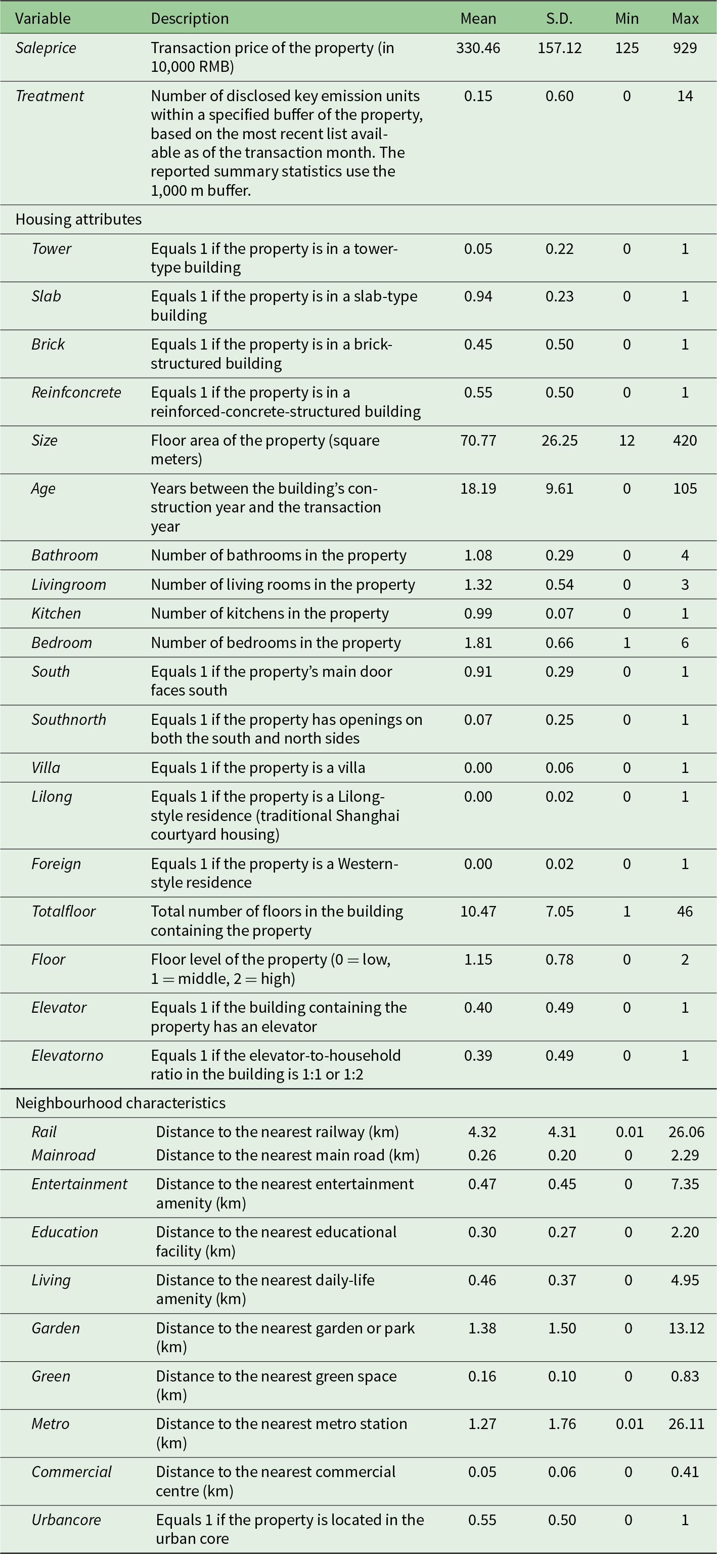
Table 2 Long description
The table lists each variable with its definition, mean, standard deviation, minimum and maximum. Saleprice, the transaction price in 10,000 RMB, has mean of 330.46 (SD: 157.12, range 125–929). Treatment, the number of disclosed key emission units within 1,000 m of the property, has mean of 0.15 (SD: 0.60, range 0–14). Housing attributes include building type (94 per cent slab), structure (55 per cent reinforced concrete), floor area (mean 70.77 square meters), age (mean 18.19 years), number of bathrooms, living rooms, kitchens and bedrooms, orientation (91 per cent south-facing), total floors, floor level and elevator access (40 per cent). Neighbourhood characteristics are straight-line distances in kilometres to the nearest railway, main road, entertainment, education, daily-life amenity, garden, green space, metro station and commercial centre, plus an urban-core indicator (55 per cent of properties are in the urban core).
Note: Each observation is a property transaction in the grouped repeated cross-sectional dataset. Data cover 2015–2022 and are cleaned as described in the text. Transaction price is measured in 10,000 RMB. Treatment counts disclosed key emission units within a 1,000 m buffer of the property as of the transaction month, based on the most recent disclosure list; transactions before the first list are assigned zero. Distance variables are straight-line distances (km) to the nearest amenity. Control variables include time-invariant housing attributes (e.g., structure, size and age) interacted with year and time-varying neighbourhood characteristics.
In terms of spatial distribution, Figure 2 maps the yearly locations of key emission units (colour-graduated red stars), which are concentrated in suburbs and industrial zones around the urban core (black clusters) and beyond the green-line urban-core boundary. This legacy industrial siting provides variation for suburban versus urban-core heterogeneity tests and underscores the policy's relevance as Shanghai expands towards industrial peripheries.
Spatial distribution of key emission units and repeated cross-sectional data in Shanghai from 2015 to 2022.

Figure 2 Long description
Panel (a) has pollution types in rows (air, soil, water, hazardous waste, other) and years 2017 to 2022 in columns. The annual number of listed key emission units rises from 160 in 2017 to 995 in 2018, 1,255 in 2019, 1,461 in 2020, 1,733 in 2021 and 1,713 in 2022, for a total of 7,317. Water units are the largest category (2,198), followed by hazardous waste (1,876), air (1,585), soil (1,057) and other (601). Panel (b) has treatment levels 0 to 14 in rows, where treatment is the number of key emission units within 1,000 m of a transaction, and calendar years 2015 to 2022 in columns. Of 98,860 transactions in total, 90,609 have treatment 0. Treated transactions first appear in 2016 (38 transactions) and grow over time. Treatment level 1 is the most common treated level with 4,756 transactions overall, and levels above 5 are rare.
Overall, the grouped repeated cross-sectional sample provides substantial variation in treatment timing and intensity across Shanghai's diverse urban landscape, enabling identification of dynamic capitalization effects while controlling for time-invariant unobservables and supporting policy-relevant heterogeneity analyses.
4. Empirical methods and identification
We estimate the causal effect of Shanghai's key emission unit list disclosure on house prices using a repeated cross-sectional TWFE model with staggered DID. We then extend it with the heterogeneity-robust estimator of de Chaisemartin and D'Haultfœuille (Reference de Chaisemartin and D'Haultfœuille2020), which accommodates treatment status changing during the study period. These approaches use panel-like data and exploit within-group variation from 2015 to 2022 to control for time-invariant group-level unobserved heterogeneity.
4.1. Baseline TWFE repeated cross-sectional model
To mitigate omitted-variable bias, we construct repeated cross-sectional data within groups that are identical in attributes except for transaction timing and price. Following prior studies (Chen et al., Reference Chen, Glaeser and Wessel2023; Hur and Kim, Reference Hur and Kim2023), we specify the baseline TWFE model as follows:
 \begin{equation}lnSaleprice_{iget}=\beta_1+\beta_2 Treatment_{iget}+X_{it}^{\prime}\theta+\mu_g+\gamma_e+\delta_t+\lambda_dt+\varepsilon_{iget,}\end{equation}
where 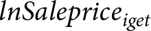 $lnSalepric{e_{iget}}$ is the log of the sale price for house transaction
 $i$ in group
 $g$ in event year
 $e$ and calendar year
 $t$;
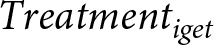 $Treatmen{t_{iget}}$ is the number of disclosed key emission units within a given distance buffer around house transaction
 $i$ in group
 $g$ in event year
 $e$ and calendar year
 $t$, capturing both spatial proximity and disclosure timing. Treatment carries the subscript
 $i$ because the de Chaisemartin and D'Haultfœuille (Reference de Chaisemartin and D'Haultfœuille2020) estimator allows non-binary and non-absorbing treatment, so treatment exposure may vary across transactions within the same group. We define the event year (disclosure year) based on the relative timing between the transaction month and the list release months. Transactions within one year before the first release are assigned to event year 0, those between one and two years before to event year −1, and so on. For transactions in or after the first list release, the period from the first release month to the month before the second is event year 1, from the second release month to the month before the third is event year 2, and so forth. Based on this month-level timing structure, each housing transaction is then matched to the most recent list released in or before the transaction month, and
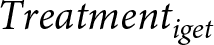 $Treatmen{t_{iget}}$ is then constructed as the number of disclosed key emission units within the specified buffer around that transaction. If a transaction occurs before the first available list, the treatment count is set to zero. This measure therefore captures both fine disclosure timing and time-varying treatment exposure as units enter or exit the annual lists.
 ${X_{it}}$ denotes time-varying controls, including time-invariant housing attributes interacted with year and time-varying neighbourhood characteristics. This interaction allows the hedonic prices of housing characteristics to vary over time (Beltrán et al., Reference Beltrán, Maddison and Elliott2019).
 ${\mu _g}$ are group fixed effects which absorb time-invariant observables and unobservables;
 ${\gamma _e}$ are event year fixed effects controlling for disclosure year variations;
 ${\delta _t}$ are year fixed effects controlling for market-wide shocks;
 ${\lambda _d}t$ are district-specific linear time trends to control for heterogeneous trends across Shanghai's districts and
 ${\varepsilon}_{{iget}}$ is the error term, clustered at the group level.
The coefficient  ${\beta _2}$ identifies the average effect per unit, assuming parallel trends and no anticipation. Unlike binary treatments and absorbing treatments, this non-binary ordered measure varies annually with listings and delistings, enabling analysis of reversible exposure.
4.2. Heterogeneity-robust extensions
Key emission units are disclosed annually, creating staggered treatment timing across house transactions. This staggered treatment structure requires strong a priori assumptions in standard TWFE models, and consistent estimates emerge only under homogeneous effects (de Chaisemartin and D'Haultfœuille, Reference de Chaisemartin and D'Haultfœuille2020; Callaway and Sant'anna, Reference Callaway and Sant'anna2021; Goodman-bacon, Reference Goodman-bacon2021; Sun and Abraham, Reference Sun and Abraham2021; Borusyak et al., Reference Borusyak, Jaravel and Spiess2024). As Goodman-bacon (Reference Goodman-bacon2021) illustrates, TWFE estimates are a weighted average of all possible 2 × 2 DID comparisons between groups treated at different times. The TWFE estimator identifies the average treatment effect on the treated only when treatment effects are homogeneous across groups and periods.
Because the key emission unit list is reviewed annually, units on the list may remain listed or be removed after improved performance. Thus, treatment status and intensity can change over time, and treatment is not necessarily absorbing (once treated, always treated). We therefore do not use the Callaway and Sant'anna (Reference Callaway and Sant'anna2021) or Wooldridge (Reference Wooldridge2021) estimators, which cannot fully accommodate non-absorbing treatment. Instead, we use the heterogeneity-robust estimator introduced by de Chaisemartin and D'Haultfœuille (Reference de Chaisemartin and D'Haultfœuille2020), the dCDH estimator, to estimate the baseline TWFE model while addressing treatment-effect heterogeneity. The dCDH estimator compares groups switching from untreated in  $t - 1$ to treated in
 $t$ with groups untreated in both periods, and groups switching from treated in
 $t - 1$ to untreated in
 $t$, with groups treated in both periods. These comparisons provide a consistent estimate of the average treatment effect. Furthermore, the estimator also allows non-absorbing states and non-binary treatments, making it well suited to our setting.
The dCDH estimator can be extended to non-binary ordered treatments without changing the assumptions required for binary treatment. Although we also report estimates for a binary indicator equal to one if at least one disclosed unit lies within 1,000 m of the transaction in its event year, our baseline specification uses the dCDH estimator with a non-binary ordered treatment. This preserves variation in treatment intensity from both new listings and delistings, rather than collapsing exposure into a simple treated-versus-untreated indicator. The honest DID sensitivity analysis of Rambachan and Roth (Reference Rambachan and Roth2023), reported in Supplementary Appendix D, shows that the baseline estimate remains robust to moderate post-treatment deviations from parallel trends.
5. Results
We present empirical findings on the capitalization effects of key emission unit disclosure in several steps. We begin with baseline estimates from the repeated cross-sectional TWFE model across alternative distance buffers. We then turn to the baseline heterogeneity-robust estimator of de Chaisemartin and D'Haultfœuille (Reference de Chaisemartin and D'Haultfœuille2020), comparing binary and ordered treatment definitions and examining dynamic treatment effects. We further assess spatial decay across distance buffers to justify the 1,000 m baseline. Finally, we explore heterogeneity by urban-core versus suburban location and by pollution type.
5.1. Repeated cross-sectional TWFE results
Table 3 reports baseline TWFE estimates of the effect of annual key emission unit disclosure on housing prices, for the number of disclosed key emission units within distance buffers of 500, 1,000, 1,500 and 2,000 m. For each buffer, the first column excludes housing-attribute and neighbourhood-characteristic controls, while the second includes them.
Baseline TWFE results
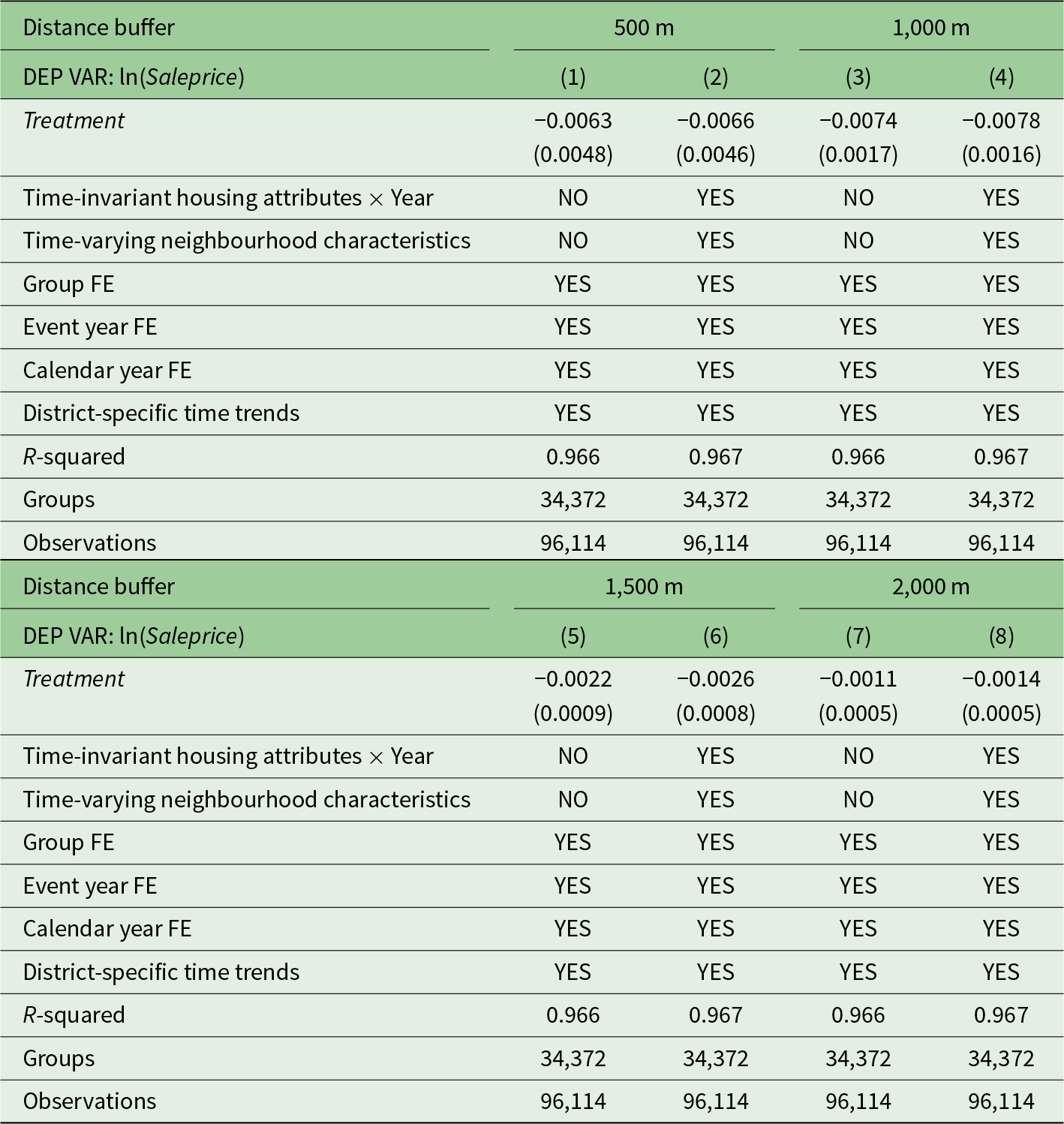
Table 3 Long description
Eight columns report TWFE estimates of treatment, the number of disclosed key emission units within the buffer, on log transaction price. All specifications include group, event-year and calendar-year fixed effects and district-specific time trends; even-numbered columns add time-invariant housing attributes interacted with year and time-varying neighbourhood controls. Coefficients (robust standard errors) are: 500 m buffer, −0.0063 (0.0048) and −0.0066 (0.0046); 1,000 m, −0.0074 (0.0017) and −0.0078 (0.0016); 1,500 m, −0.0022 (0.0009) and −0.0026 (0.0008); 2,000 m, −0.0011 (0.0005) and −0.0014 (0.0005). Effects are negative at all buffers, statistically significant at 1,000 m and beyond and shrink in magnitude as the buffer widens. R-squared is about 0.97 in all columns, with 34,372 groups and 96,114 observations.
Note: This table reports baseline TWFE estimates from the empirical model (1) for varying distance buffers. The dependent variable is the log transaction price of a property. Treatment is the number of disclosed key emission units located within each distance buffer in a given event year. Within each buffer, the odd-numbered column reports estimates without additional controls, while the even-numbered column adds time-invariant housing attributes interacted with year and time-varying neighbourhood characteristics. All specifications include group fixed effects, event-year fixed effects, calendar-year fixed effects and district-specific linear time trends. Robust standard errors are reported in parentheses.
We find three main results. First, housing prices decrease significantly when more key emission units are disclosed within the buffer. For the 1,000 m buffer, one additional disclosed unit is associated with a 0.78 per cent house price decrease. Second, the estimated effect generally attenuates as the buffer expands. The 500 m estimate is statistically insignificant, likely reflecting the small number of housing transactions close to key emission units, which are often located in industrial areas with limited nearby residential activity (only 1,538 exposed transactions at the 500 m buffer versus 8,251 at 1,000 m). Finally, adding housing-attribute and neighbourhood controls does not substantially change the estimates.
5.2. Baseline estimator and dynamic effects
To address heterogeneous treatment effects in the baseline TWFE model, we use the staggered heterogeneity-robust DID estimator of de Chaisemartin and D'Haultfœuille (Reference de Chaisemartin and D'Haultfœuille2020). Table 4 compares baseline TWFE estimates (columns (1) and (3)) with baseline dCDH estimates (columns (2) and (4)) using a 1,000 m buffer. Columns (1) and (2) use the binary treatment definition, while columns (3) and (4) use the non-binary ordered treatment definition. All specifications include time-invariant housing attributes interacted with year, time-varying neighbourhood characteristics and all fixed effects. For comparison, Supplementary Appendix Table A3 reports the corresponding TWFE and dCDH estimates without the time-varying controls, with similar results.
TWFE and de Chaisemartin and D'Haultfœuille (Reference de Chaisemartin and D'Haultfœuille2020) estimation results

Table 4 Long description
Four columns use a 1,000 m buffer. Columns 1 and 2 use a binary treatment equal to one if at least one disclosed key emission unit is within 1,000 m of the housing transaction: the TWFE estimate is −0.0091 (SE 0.0029) and the dCDH average cumulative effect is −0.0242 (0.0066). Columns 3 and 4 use an ordered treatment counting nearby units: the TWFE estimate is −0.0078 (0.0016) and the dCDH estimate is 0.0131 (0.0036). Pre-trend placebo joint tests do not reject zero (p-values 0.142 and 0.1328). Robust standard errors clustered at the group level are reported in parentheses for the TWFE estimates. Bootstrapped standard errors clustered at the group level are reported in parentheses for the dCDH estimates. All columns include full controls, group, event-year and calendar-year fixed effects, as well as district-specific time trends. TWFE uses 96,114 observations; the dCDH estimates use 41,481 and 41,290 observations with 1,524 and 1,664 switch-by-period observations.
Note: This table compares baseline TWFE estimates with estimates from the de Chaisemartin and D'Haultfœuille (Reference de Chaisemartin and D'Haultfœuille2020) DID estimator using a 1,000 m treatment buffer. The dependent variable is the log transaction price of a property. Columns (1) and (3) report conventional TWFE estimates, while columns (2) and (4) report estimates from the dCDH estimator. Columns (1) and (2) use a binary treatment indicator equal to one if at least one disclosed key emission unit in the event year of the housing transaction is located within 1,000 m of that transaction. Columns (3) and (4) use an ordered treatment variable measuring the number of disclosed key emission units located within 1,000 m of each property transaction in the event year of that transaction. For the dCDH estimates, the reported coefficient is the average cumulative effect of the binary or ordered treatment. The Pre-Trend Placebo Joint Test p-value reports the p-value from the joint test that the three placebo estimates are equal to zero. N reports the number of observations used to estimate the average cumulative effect. Switch  $ \times $ Periods reports the number of switch-by-period observations to which the average cumulative effect applies. Robust standard errors clustered at the group level are reported in parentheses for the TWFE estimates. Bootstrapped standard errors clustered at the group level are reported in parentheses for the dCDH estimates.
The estimates are negative and statistically significant across both treatment definitions and estimators. The baseline dCDH estimate is substantially larger than the baseline TWFE estimate, suggesting that TWFE may understate the capitalization effects of key emission unit disclosure when treatment effects are heterogeneous. For the binary treatment, the heterogeneity-robust estimate indicates an average cumulative decrease of approximately 2.42 per cent for properties exposed to at least one disclosed key emission unit within 1,000 m. For the non-binary ordered treatment, the dCDH estimate in column (4) implies that each additional disclosed key emission unit within 1,000 m reduces nearby housing prices by approximately 1.31 per cent. This magnitude is close to the 1.84 per cent effect of environmental punishment disclosures on Beijing house prices (Agarwal et al., Reference Agarwal, Ding, Kuang and Zhu2023).
The dCDH estimator also provides placebo tests for parallel pre-trends. These tests simulate policy implementation in periods  $t - 1$ to
 $t - 3$ and compare outcomes with periods without actual implementation. As shown in columns (2) and (4) of Table 4, the placebo estimates are statistically insignificant and reveal no detectable differential pre-trends.
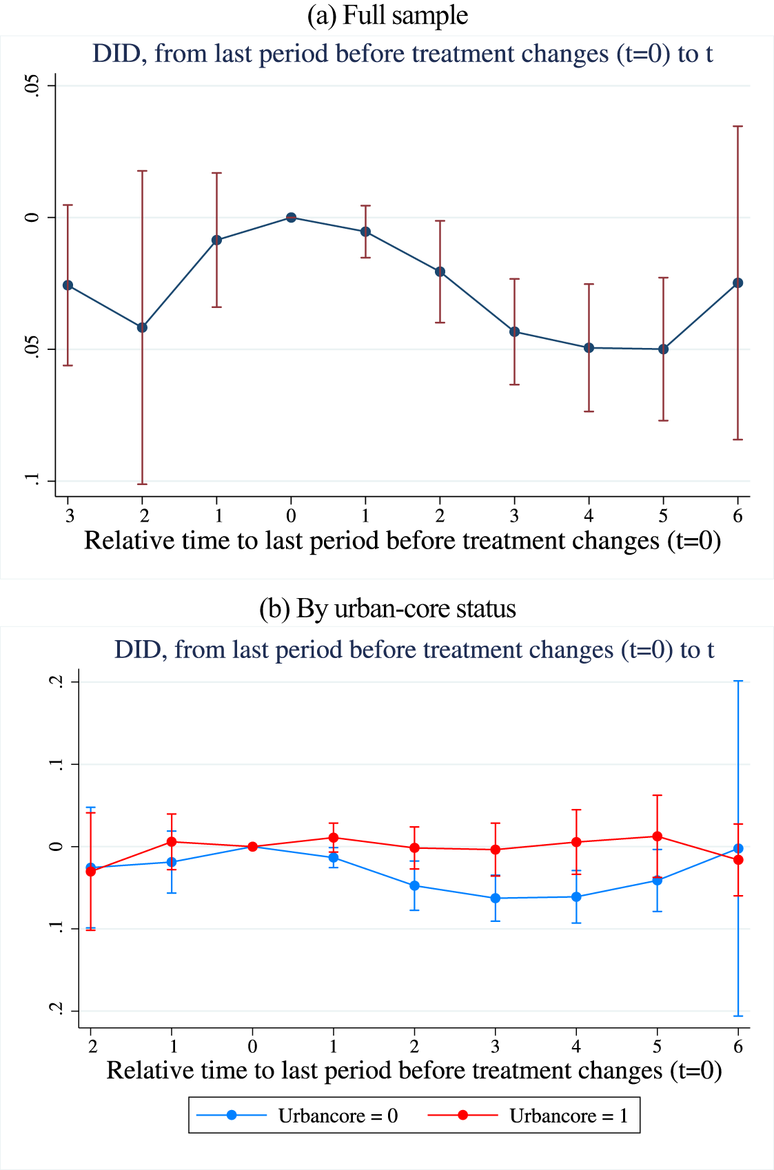
The dCDH estimator also provides dynamic heterogeneity-robust treatment effects. Figure 3a shows the dynamic effects for the ordered treatment definition, where treatment counts disclosed key emission units within a 1,000 m buffer. The specification includes the same controls, fixed effects and district-specific time trends as the baseline model. The pre-treatment placebo estimates at 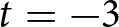 $t = - 3$ to
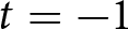 $t = - 1$ are not statistically different from zero, further supporting the absence of differential pre-trends. The coefficient in the first period after a treatment change,
 $t = 1$, is negative but not statistically significant.Footnote 8 This may reflect buyers and sellers entering purchase contracts before disclosure even when the transaction closing occurred after disclosure. The effects become statistically significant from
 $t = 2$ and larger in magnitude from
 $t = 3$ to
 $t = 5$, suggesting the capitalization effect strengthens over time. By
 $t = 6$, the point estimate remains negative, but the confidence interval widens and includes zero.
Dynamic treatment effects using a heterogeneity-robust estimator.

Figure 3 Long description
Two event–study panels plot dCDH estimates of the dynamic effects of key emission unit disclosures on log housing prices. The x–axis is relative time from the last period before a treatment change, normalized to zero; the y–axis is the estimated change in log prices. Points are estimates and vertical bars are 95 per cent confidence intervals. Panel (a) shows the full sample, with post–treatment estimates declining to about minus 0.05. Panel (b) splits the sample by urban–core status: estimates outside the urban core turn negative after treatment, while urban–core estimates stay near zero.
We also apply the dCDH estimator across different distance buffers. Supplementary Appendix Table A4 shows the average cumulative effects, which indicate a distance-decay pattern. The negative effect is largest in magnitude at 500 m and declines as the buffer expands, although the 2,000 m estimate is statistically insignificant. This suggests the capitalization effect of key emission unit disclosure is spatially localized. Significant pre-trend placebo joint tests suggest the 500 and 2,000 m buffers are more vulnerable to identification concerns. The 500 m estimates may be sensitive to limited switcher-period observations (432 in Supplementary Appendix Table A4) and local composition differences near industrial areas, whereas the 2,000 m treatment definition may be too broad and may capture additional spatial confounders. The evidence is strongest for the intermediate buffers (750, 1,000 and 1,500 m), where effects are negative and placebo tests do not reject parallel pre-trends. We therefore use the 1,000 m buffer as the baseline specification.
5.3. Spatial heterogeneity
Key emission units are often located in suburban areas as urban expansion has spread to previously industrial areas, so disclosure impacts there may differ from those in the urban core. To test this, we use Shanghai's Outer Ring Expressway to divide the data into urban-core and suburban subsamples.Footnote 9 Using the de Chaisemartin and D'Haultfœuille (Reference de Chaisemartin and D'Haultfœuille2020) estimator, we estimate dynamic treatment effects of the non-binary treatment separately for each subsample. Because the sample is split and includes a large number of controls and fixed effects, the suburban subsample has too few switchers to estimate the same three pre-treatment placebo periods used in previous sections. We therefore estimate two pre-treatment placebo periods for both subsamples.
Figure 3b presents the heterogeneity-robust treatment estimation results, using a 1,000 m treatment buffer and time-varying controls. Both subsamples reveal no detectable differential pre-trends in the placebo test. After disclosure, estimates for urban-core properties remain close to zero and generally statistically insignificant throughout the post-treatment period. In contrast, properties outside the urban core experience larger and more persistent negative effects. Consistent with this pattern, the average cumulative effect estimates reported in Supplementary Appendix Table A5 are larger in magnitude for the suburban subsample than for the urban-core subsample. This suggests the disclosure of key emission units has a greater and more prolonged negative effect on suburban than on urban-core property prices. Given that urban-core housing typically has more amenities and higher demand than suburban housing, this asymmetric impact implies that the disclosure policy may further widen the urban-suburban housing price gap in Shanghai.
5.4. Pollution heterogeneity
SMBEE reports the pollutant types associated with each disclosed key emission unit, in five categories: air, water, soil, hazardous waste and other. This classification allows us to examine whether disclosure effects vary by pollutant type. Because some units are associated with multiple pollutant types and hazardous waste information was not disclosed in 2017 and 2018, we merge hazardous waste and other types into a single group, yielding four pollutant types for analysis. The soil-pollutant specification lacks sufficient switchers for three pre-treatment placebo periods, so we estimate two pre-treatment placebo periods for this type.
Supplementary Appendix Table A6 examines heterogeneity by key emission unit type using the de Chaisemartin and D'Haultfœuille (Reference de Chaisemartin and D'Haultfœuille2020) estimator with a 1,000 m treatment buffer. The negative capitalization effect is concentrated among water and soil key emission units. The average cumulative effects are −0.0260 for water and −0.0307 for soil units, implying approximately 2.60 and 3.07 per cent decreases in nearby house prices, respectively. In contrast, the estimates for air and other units are statistically insignificant. The dynamic estimates in Supplementary Appendix Figure A2 are broadly consistent, with water and soil units showing more persistent negative post-treatment patterns. Placebo joint tests do not reject the null of no differential pre-trends in any of the four specifications. Overall, market responses to disclosure are stronger for water- and soil-related units, reflecting the more localized and persistent environmental risks they pose. For air-related units, emissions may be more spatially diffuse and harder for homebuyers to attribute to a specific nearby source.
6. Robustness tests
6.1. Delisting of key emission units
SMBEE updates the list of key emission units annually. Some new units are added, while previously listed units either remain or are delisted. Because the de Chaisemartin and D'Haultfœuille (Reference de Chaisemartin and D'Haultfœuille2020) estimator allows treatment entry and exit and does not require treatment status to be absorbing, the estimates combine the listing and delisting effects. This section examines delisting separately.
We assume that key emission units may be delisted through two mechanisms: (a) firms moving away, or (b) firms reducing pollution levels. To examine this, we identify delisted units by keyword-matching unit names across adjacent annual lists. We then use the website Qichacha (‘企查查’) to check whether these delisted units changed production addresses, and whether the address change occurred between the release dates of the two adjacent lists (Qichacha, 2026). As shown in Supplementary Appendix Table A7, only 10 of 126 delisted units moved away, and only 2 of those moved before the delisting was publicly disclosed. Moving away is thus unlikely to be the primary delisting mechanism, and reducing pollution levels is the more plausible channel. This is also consistent with practical constraints in China, where relocating production typically requires complex government approval and can be costly.
Although delisting due to firm relocation appears uncommon, delisting itself may still affect nearby housing prices and confound the baseline results, which do not distinguish listings from delistings. We therefore treat delisting as a standalone analysis. Specifically, we define treatment as the number of delisted key emission units within the baseline 1,000 m buffer of each housing transaction in a given event year. Delisted units are those that appear on the list in year t − 1 but not in year t. We then estimate the baseline model using the dCDH estimator. Supplementary Appendix Table A8 shows no statistically significant effect of delisting: the dCDH estimates are small and positive (0.0079 without controls, 0.0078 with controls) and statistically insignificant. Pre-trend placebo joint tests fail to reject the null (p-values 0.4823 and 0.3521). Thus, these results provide little evidence that delisting by itself raises nearby housing prices, suggesting that the baseline results are unlikely to be driven by delisting.
6.2. Key emission unit disclosure without delisting
Although the previous section suggests that key emission units are unlikely to avoid environmental regulation by relocating, delisting through compliance and lower emissions may improve local environmental quality and increase nearby housing prices. To remove this confounder, we exclude units that are delisted in the following year, as well as nearby transactions, and re-estimate the baseline regressions (Supplementary Appendix Table A9).
Supplementary Appendix Table A9 shows that the negative disclosure effect persists after excluding delisted key emission units and nearby transactions. Relative to the baseline estimates in columns (1) and (2), the estimates in columns (3) and (4) become larger in magnitude, rising from −0.0114 to −0.0169 without controls and from −0.0131 to −0.0194 with controls, consistent with delisting-related improvements partially offsetting the baseline disclosure effect. All estimates remain statistically significant, and the pre-trend placebo joint tests remain insignificant. These findings indicate that the baseline dCDH estimator captures the overall effect of list disclosure, including newly listed, continuing and later-delisted units.
6.3. Misassigned treatment under Callaway and Sant'anna (Reference Callaway and Sant'anna2021) and Wooldridge (Reference Wooldridge2021) assumptions
The Callaway and Sant'anna (Reference Callaway and Sant'anna2021) and Wooldridge (Reference Wooldridge2021) estimators assume absorbing treatment: once a unit is exposed to the policy, it remains treated in all subsequent periods. This is inconsistent with our setting, where the key emission unit lists change annually, and units may enter or exit, generating time-varying exposure. This motivates our use of the dCDH estimator, which explicitly allows treatment entry and exit. To compare our results with estimates based on the absorbing-treatment assumption, we construct a misassigned treatment variable imposing an artificial absorbing state. Any unit that enters the list is assumed to remain listed in all subsequent years, even if removed from the actual list. This simulates a ‘once treated, always treated’ scenario and allows direct comparison with the Callaway and Sant'Anna and Wooldridge estimates reported in Supplementary Appendix C.
This misassignment affects the original treatment assignment in two ways. First, for some houses, the number of nearby key emission units in certain years changes from zero to one, introducing treatment status in years when no treatment actually occurred. Second, for properties already exposed to treatment, treatment intensity increases because units that should have been dropped from the list remain included. To avoid confounding these two changes, we construct both binary and ordered misassigned treatment variables under the absorbing treatment assignment. The binary indicator equals one if at least one disclosed unit is located within 1,000 m of a transaction. The ordered misassigned treatment variable measures the number of disclosed units within 1,000 m of a transaction. Both are estimated using the dCDH estimator, following baseline Equation (1).
Supplementary Appendix Table A10 reports dCDH estimates using misassigned treatment variables under an artificially imposed absorbing-treatment assumption. The estimates for both binary misassigned treatment (−2.36 per cent) and ordered misassigned treatment (−1.39 per cent) are close to the baseline dCDH estimates (−2.42 per cent for binary treatment and −1.31 per cent for ordered treatment). The differences are less than 0.1 percentage points, suggesting that estimates based on the misassigned treatment assignment are similar to those based on the actual treatment assignment. This finding suggests that homebuyers may not closely track whether key emission units are delisted across years; instead, they respond primarily to the fact that information about nearby key emission units has been disclosed and remains publicly available online.
6.4. Frequently transacted Xiaoqu (residential complex)
Shanghai, as China's most economically developed city, has a highly regulated real estate market. The city also imposes strict purchase restrictions on homebuyers.Footnote 10 These restrictions should not affect our estimates of key emission unit disclosure effects, as long as enough market participants generate an equilibrium. If sufficient transactions still occur to form an observable housing market equilibrium, these strict purchase restrictions should not eliminate the underlying marginal willingness to pay for environmental quality.
However, if the restrictions are too stringent, some areas of Shanghai may have too few buyers for full sorting behaviour to be observed, which could lead us to underestimate the effect of key emission unit disclosure. As a robustness check, we focus on areas in Shanghai with relatively frequent housing transactions. We rank Xiaoqu in the final analysis sample by transaction count and re-estimate the baseline regression using subsamples restricted to Xiaoqu in the top 50, 75 and 80 per cent of the transaction-count distribution. Supplementary Appendix Table A11 shows that the estimated average cumulative effects are negative and statistically significant in all three subsamples, with coefficients of −0.0128, −0.0147 and −0.0146 for Xiaoqu above the 50th, 75th and 80th percentiles, respectively.
These estimates are very close to the baseline dCDH estimate (−0.0131). The 75th- and 80th-percentile estimates are slightly larger but do not change the conclusion of a negative capitalization effect. Supplementary Appendix Figure A3 also reports dynamic treatment effects for all three subsamples, which are consistent with the baseline dCDH dynamic results. Taken together, our main findings are robust in more actively traded Xiaoqu. Their transaction prices are more likely to reflect equilibrium under Shanghai's strict regulations.
7. Conclusion and discussion
We advance understanding of the market effects of environmental disclosure policies by providing the first causal estimates of Shanghai's key emission unit disclosure program on housing prices. Using grouped repeated cross-sectional data and heterogeneity-robust staggered DID estimators, we identify significant negative capitalization effects from annual unit disclosures. One additional disclosed unit within 1,000 m reduces nearby housing prices by 1.31 per cent, and the effect increases to 1.94 per cent when delisted units are excluded. The effects are localized between 750 and 1,500 m, absent in the disclosure year and persistent over the following four years, from  $t = 2$ through
 $t = 5$. Suburban properties experience larger price declines than urban-core properties, which may widen spatial price disparities. The effects are also larger for water and soil pollution types. Most units do not delist through relocation, and delisting itself has no statistically significant effect on nearby prices. Robustness checks using treatment assignment without delisting, misassigned treatment, alternative heterogeneity-robust estimators, frequently transacted Xiaoqu subsamples and honest DID sensitivity analysis support the baseline findings.
These results extend prior U.S. and Chinese literature. U.S. studies on the TRI emphasize perceived risks driving localized declines but often focus on legacy contamination or one-time events. We shift attention to ongoing industrial pollution in a dynamic annual framework, providing suggestive evidence of delayed price adjustment that emissions changes alone are unlikely to explain. In China, existing work documents short-term price declines from environmental punishments (Zheng and Kahn, Reference Zheng and Kahn2013) or specific contaminants (Wang and Yang, Reference Wang and Yang2024), but it overlooks multi-pollutant and reversible disclosure regimes. By aggregating broad industrial sources and modelling non-absorbing treatment, we identify dynamics that are overlooked in NIMBY-focused analyses. Methodologically, adapting de Chaisemartin and D'Haultfœuille (Reference de Chaisemartin and D'Haultfœuille2020) to ordered, reversible treatment and validating the estimates with Rambachan and Roth (Reference Rambachan and Roth2023) strengthens causal inference in staggered settings and offers a template for evaluating similar policies. The Shanghai context also provides external validity for other rapidly developing cities where flexible residential mobility allows households to respond to disclosed information through housing choices.
As part of a nationwide mandate, Shanghai's implementation of the policy suggests that disclosure can reduce information frictions and affect housing choices. The average decline of 1.31 per cent corresponds to meaningful equity losses, roughly 40,019 RMB per affected property at mean prices, and may erode suburban wealth as cities expand into industrial zones. This asymmetry cautions against uniform policies and calls for targeted support in vulnerable areas, such as subsidies or enhanced monitoring to accelerate the benefits of delisting. Broader dissemination through media and platforms such as SEIDP amplifies these effects, as our awareness metrics suggest, indicating that transparency investments can yield high returns. Integrating disclosure with incentives such as emissions trading could further amplify pollution reductions and strengthen corporate accountability beyond command-and-control regulation.
Supplementary material
The supplementary material for this article can be found at https://doi.org/10.1017/S1355770X26100771.
Competing interests
The authors declare no competing interests.





 Open access

