1 Introduction
Many hydrodynamic applications, such as turbopumps, ship propellers, hydroturbines or diesel injectors, are required to operate in regimes where cavitation cannot be avoided. Frequently, it is encountered as partial cavitation, i.e. when the cavity closes on the surfaces of a flow obstacle. In general, partial cavitation is a highly unsteady phenomenon. As Callenaere et al. (Reference Callenaere, Franc, Michel and Riondet2001) pointed out, two fundamental sources of unsteadiness can be distinguished. First, ‘system instabilities’ denote unsteady behaviour due to the interaction of the cavity volume with the surrounding system. Second, ‘intrinsic instabilities’ render the cavity inherently unsteady, even under steady operating conditions.
In its most violent form, partial cavitation is associated with the periodic shedding of large vapour clouds. A comprehensive discussion of this flow regime was given, for example, by Reisman, Wang & Brennen (Reference Reisman, Wang and Brennen1998) and Laberteaux & Ceccio (Reference Laberteaux and Ceccio2001). It is characterised by a variety of cavitation topologies, including sheet, cloud as well as vortex cavitation, and involves various length and time scales. Cavitating vortices range from small-scale turbulent eddies, to larger streamwise-oriented structures, known as ‘streamers’ (Laberteaux & Ceccio Reference Laberteaux and Ceccio2001), to cavitating horseshoe vortices, which can reach the extent of the original sheet cavity itself, or fractions thereof. Further characteristic patterns are ‘crescent-shaped regions’ and ‘leading-edge structures’ (Reisman et al.
Reference Reisman, Wang and Brennen1998). While the length scale of global cavity structures is of the order of the characteristic scales of the flow obstacle, cavity clouds consist of numerous bubbles of various sizes. By performing off-axis laser holography of cloud cavitation on a two-dimensional hydrofoil, Kato et al. (Reference Kato, Yamaguchi, Maeda, Kawanami and Nakasumi1999) were able to detect bubbles down to a radius of
 $10~\unicode[STIX]{x03BC}\text{m}$
. The authors reported that the number density for bubbles with radii of
 $35~\unicode[STIX]{x03BC}\text{m}$
or larger is of the order of
 $10^{3}~\text{bubbles}~\text{cm}^{-3}$
.
Cloud cavitation results in large fluctuations of cavity volume, causing strong variations in lift and drag forces. Wade & Acosta (Reference Wade and Acosta1966), studying unsteady cloud cavitation on a plano-convex hydrofoil, reported on lift oscillations reaching up to
 $\pm 10\,\%$
of the steady mean. For the case of a two-dimensional NACA 0015 hydrofoil, Arndt et al. (Reference Arndt, Song, Kjeldsen and Keller2001) later found variations in the lift exceeding the mean by 100 %. Consequently, cloud cavitation may also lead to substantial structural vibrations. Many researches have shown that surface pressure loads are extremely high for this regime; refer, e.g., to Le, Franc & Michel (Reference Le, Franc and Michel1993) and Kawanami et al. (Reference Kawanami, Kato, Yamaguchi, Tanimura and Tagaya1997). Reisman et al. (Reference Reisman, Wang and Brennen1998) identified propagating shock waves emitted during ‘local’ and ‘global events’ as the fundamental reason for these pressure fluctuations. Due to the violent nature of the collapses, cloud cavitation is not only associated with severe levels of noise, but is also considered as one of the most aggressive forms of cavitation (Gopalan & Katz Reference Gopalan and Katz2000).
Due to these detrimental implications, it is of primary interest (i) to investigate the transition from stable cavities to the unsteady shedding of clouds, (ii) to identify relevant mechanisms governing the dynamics of cloud cavitation and, possibly, (iii) to deduce effective means for flow control. In the classical view, cloud cavitation is associated with the occurrence of a re-entrant jet. Feeding an intrinsic instability mechanism, it develops at the cavity closure. Regarded as a thin upstream-propagating flow of liquid underneath the original sheet cavity, it displaces the cavity away from the wall. When it intersects again with the vapour–liquid interface close to the leading edge, it pinches off the sheet, thereby generating a newly detached cloud. One of the earliest experimental observations of re-entrant jets was reported by Knapp (Reference Knapp1955). High-speed videos were used to investigate the cavitating flow over two-dimensional and axisymmetric bodies. Furness & Hutton (Reference Furness and Hutton1975), utilising two-dimensional unsteady potential flow analysis, were among the first to predict the re-entrant jet phenomenon by analytical models. Later, many experimental studies followed, which identified the re-entrant jet as the driving mechanism for sheet-to-cloud transition; see, e.g., the works of Wade & Acosta (Reference Wade and Acosta1966), Lush & Skipp (Reference Lush and Skipp1986) and Foeth, van Terwisga & van Doorne (Reference Foeth, van Terwisga and van Doorne2008). Kawanami et al. (Reference Kawanami, Kato, Yamaguchi, Tanimura and Tagaya1997), studying re-entrant-jet-induced cloud cavitation over an elliptic-nose hydrofoil, demonstrated an effective means of passive flow control. By placing a small obstacle perpendicular to the direction of the flow, the re-entrant jet can be stopped, thereby suppressing the associated cloud cavitation. The same conclusion was drawn by Pham, Larrarte & Fruman (Reference Pham, Larrarte and Fruman1999) in a similar study for a plano-convex hydrofoil. By preventing the shedding of large-scale vapour clouds, it allows the effective mitigation of flow aggressiveness and, thus, cavitation erosion. As a positive side effect, Kawanami et al. (Reference Kawanami, Kato, Yamaguchi, Tanimura and Tagaya1997) also reported on the reduction of emitted noise and hydrofoil drag.
As early as 1964, Jakobsen (Reference Jakobsen1964) speculated that the observed violent head breakdown in cavitating inducers is caused by a different mechanism. He conjectured that the two-phase mixture locally reaches a supersonic state such that shock phenomena occur in the cavitating flow. However, no direct experimental observation was made by the author. Similarly, Kawanami et al. (Reference Kawanami, Kato, Yamaguchi, Tanimura and Tagaya1997) also reported on a condensation shock phenomenon, but eventually concluded that cloud shedding is related to a re-entrant jet.
Shocks can appear in bubbly flow, since the mixture speed of sound is significantly lower than for either of the two pure constituents. Mallock (Reference Mallock1910), assuming a homogeneous mixture, was the first to derive an analytical expression for the speed of sound in a two-phase medium. One of the earliest works on the subject of propagating shock waves in bubbly flow was presented by Campbell & Pitcher (Reference Campbell and Pitcher1958), studying planar waves in gas–liquid mixtures. These authors also assumed a homogeneous mixture, and derived Rankine–Hugoniot jump conditions, thereby relating the propagation velocity of the shock to its strength. This work was later extended by Crespo (Reference Crespo1969) and Noordzij & van Wijngaarden (Reference Noordzij and van Wijngaarden1974) by also taking the relative bubble motion into account. The principal mechanisms of compressible wave propagation, e.g. steepening of compression waves, frequency dependence and oscillations in the wave structure, were identified. However, these authors considered bubbles of air immersed in liquid, and thereby excluded phase transfer. For cavitating flow, in contrast, phase transfer between the vapour and liquid needs to be taken into account. Brennen (Reference Brennen1995) and Franc & Michel (Reference Franc and Michel2005) derived analytical relations for the speed of sound in a two-phase flow. For intermediate void fractions, the speed of sound of the mixture can be up to two orders of magnitude smaller than without phase transfer. A two-phase flow with phase transition thus is more susceptible to the occurrence of shocks, and, as a consequence, the dynamics of the mixture can be significantly affected.
It is important to recall that so-called condensation shocks are distinct from shock waves emitted by collapsing cavity structures, such as bubbles or clouds. The pressure rise of collapse-induced shocks is of short duration and high amplitude, potentially reaching the order of several GPa (Philipp & Lauterborn Reference Philipp and Lauterborn1998). In contrast, condensation shocks, associated with a retracting partial cavity, act on longer time scales and involve phase change. Furthermore, with amplitudes of only a few kPa, as in the investigated case, the associated pressure rise can be very weak. Propagating through the liquid medium, collapse-induced shock waves have the potential to affect a shedding process. By abruptly stopping cavity growth when impinging on an attached sheet, as described by Arndt et al. (Reference Arndt, Song, Kjeldsen and Keller2001) and Leroux, Astolfi & Billard (Reference Leroux, Astolfi and Billard2004), this represents an external forcing of the cavity. On the other hand, condensation fronts propagate within a partial cavity. Comparable to a re-entrant jet, these fronts travel upstream through the sheet, having a velocity of the same order as the convective velocity, and cause pinch-off and subsequent shedding of vapour clouds. Yet, condensation shocks and re-entrant jets are also distinct entities, as the former involve phase change and may span the complete height of the cavity, while the latter are typically a thin layer of upstream-propagating liquid underneath the sheet.
Experimental observation of condensation shocks dictating sheet-to-cloud shedding has been described only recently in the literature. Ganesh, Mäkiharju & Ceccio (Reference Ganesh, Mäkiharju and Ceccio2016) used x-ray densitometry for visualising the instantaneous vapour volume fraction of the cavitating flow over a convergent–divergent wedge. Investigating a range of cavitation numbers, these authors discerned three regimes termed ‘incipient’, ‘transitory’ and ‘periodic’. In the first case, the shedding is dominated by a re-entrant jet, while for the latter, an upstream-propagating condensation shock is found. In the transitory regime, both phenomena alternate intermittently. The authors showed that, depending on the operation point, the time-averaged flow attains a void fraction of 5–50 %, while instantaneous values of 80–90 % or higher can be reached within the sheet cavity. Due to the low speed of sound at these void fractions, the two-phase flow supports compressible wave phenomena. Interestingly, these authors demonstrated in a subsequent study (Ganesh, Mäkiharju & Ceccio Reference Ganesh, Mäkiharju and Ceccio2015) that cloud shedding in the case of condensation shocks cannot be controlled with an obstacle located on the wedge surface.
Numerical investigations for this configuration have recently been performed by Gnanaskandan & Mahesh (Reference Gnanaskandan and Mahesh2016). Utilising compressible large-eddy simulation, these authors studied the system at a cavitation number of
 $\unicode[STIX]{x1D70E}_{1}=(p_{1}-p_{vap})/(\unicode[STIX]{x1D70C}_{ref}u_{1}^{2}/2)=2.1$
, with the upstream pressure
 $p_{1}$
, the upstream velocity
 $u_{1}$
, the vapour pressure
 $p_{vap}$
and the reference density
 $\unicode[STIX]{x1D70C}_{ref}$
. In accordance with the experiments at this operating point, corresponding to the ‘transitory’ regime, these authors observed re-entrant flow and obtained good agreement for the shedding Strouhal number. Moreover, detailed examinations of velocity and void fraction fluctuations for the sheet and cloud were provided. However, the condensation front phenomenon was not discussed by these authors.
One of the first numerical studies to examine cloud cavitation in conjunction with condensation shocks was conducted by Schmidt, Thalhamer & Schnerr (Reference Schmidt, Thalhamer and Schnerr2009). These authors used a fully compressible homogeneous mixture approach and equilibrium thermodynamics to investigate the cavitating flow past a two-dimensional NACA 0015 hydrofoil. By neglecting physical viscosity in the model, these authors discussed the condensation shock phenomenon and demonstrated that the observed cavity dynamics is essentially inertia-driven. For the same configuration, Eskilsson & Bensow (Reference Eskilsson and Bensow2012) also employed a compressible cavitation model. Comparing the results obtained with Euler, Reynolds-averaged Navier–Stokes and large-eddy simulations, these authors also noted the occurrence of such shocks.
With no direct experimental observation of condensation shocks available until recently, the authors of the aforementioned numerical studies made no attempt at a detailed inspection. The goal of the present contribution thus is to revisit this phenomenon. Relying on the numerical method developed by Schmidt et al. (Reference Schmidt, Thalhamer and Schnerr2009), the primary focus is the in-depth analysis of condensation shocks, and a validation of our predictions with the available experiments of Ganesh et al. (Reference Ganesh, Mäkiharju and Ceccio2016).
In the present study, we consider an experimental cavitation number of
 $\unicode[STIX]{x1D70E}_{1}=1.96$
, i.e. the ‘periodic’ regime. Our computational domain closely follows the experimental set-up. We account for the variation of cross-sections within the up- and downstream duct, and for the presence of the lateral walls of the test section, omitted in the previous studies by Gnanaskandan & Mahesh (Reference Gnanaskandan and Mahesh2016). Using the experimental references of Ganesh et al. (Reference Ganesh, Mäkiharju and Ceccio2016), we compare typical flow features, the global dynamics of the system and the time evolution of the shedding process. Furthermore, time-averaged and root mean square (RMS) void fraction profiles as well as instantaneous vapour volume fractions are juxtaposed.
For this study, following the methodology of Schmidt et al. (Reference Schmidt, Thalhamer and Schnerr2009), we employ a continuum approach to model the cavitating flow as a homogeneous mixture. Unresolved flow features, such as bubbles, nuclei as well as the effect of surface tension, are omitted. Furthermore, after affirming that temperature variations can be neglected, we utilise barotropic thermodynamic closures. While retaining full two-phase compressibility in the method, we deliberately omit molecular viscosity from the model. For the case of a cavitating nozzle-target flow exhibiting sheet and cloud cavitation, it has been shown previously by Mihatsch, Schmidt & Adams (Reference Mihatsch, Schmidt and Adams2015) that inviscid modelling is sufficient to capture relevant features of cavitating flow. In the present study, it is demonstrated that this is also valid when the cavity dynamics is dominated by condensation shock phenomena. Our results further provide an indication that condensation shocks, additionally to re-entrant jets, feed an intrinsic instability mechanism of partial cavities.
An inviscid model would give incorrect results for considerably lower Reynolds numbers or higher upstream pressures (corresponding to the case of incipient cavitation or single-phase flow). Viscous boundary layers, secondary flows such as corner vortices, and shear in the bulk are then important, such that viscosity cannot be neglected in these cases. The fundamental reason why an inviscid flow model is applicable for the problem at hand is that the investigated configuration is characterised by (i) a high Reynolds number, (ii) a well-defined separation line for cavitation and (iii) a low cavitation number, resulting in developed cavitation. The Reynolds-number effect was investigated experimentally by Ganesh et al. (Reference Ganesh, Mäkiharju and Ceccio2016), studying three different inlet velocities (
 $u_{1}=6,8,10~\text{m}~\text{s}^{-1}$
), corresponding to a Reynolds number based on the hydraulic diameter of the channel (
 $r_{H}=h_{ch}=76.2~\text{mm}$
) of
 $Re_{ch}=460\times 10^{3}\ldots 760\times 10^{3}$
. For the case of incipient cavitation, the authors did find a dependence on the Reynolds number, e.g. regarding the main void fraction close to the apex and the shedding Strouhal number. For the transitional and shedding cases, on the other hand, the authors qualified the Reynolds-number effect on the mean and standard deviation of the void fraction as negligible (Ganesh et al.
Reference Ganesh, Mäkiharju and Ceccio2016). Furthermore, the shedding Strouhal number and thus the dynamics of the system also does not show a Reynolds-number dependence for the investigated inlet velocities according to the experimental references. Furthermore, the pressure loss in the channel is largely dominated by the pressure imbalance caused by the cavity itself, which is not related to viscous effects.
We conclude that the rationale for an inviscid flow model in the context of the investigated configuration is threefold: well-defined separation line, developed cavitation and high Reynolds number. This situation is commonly found for engineering systems affected by cavitation. Instead of devising a general-purpose computational method, the model specifically aims at these applications. In the current context, it is employed for studying fundamental physical processes, in particular the condensation shock phenomenon.
This paper is structured as follows. The physical modelling and numerical method are discussed in § 2. In § 3, the investigated physical configuration is introduced. The computational domain, numerical grids, boundary conditions and conducted simulations are presented as well. The main results are then discussed in § 4. The paper concludes with a summary and discussion in § 5.
2 Physical model and numerical method
2.1 Model assumptions and governing equations
Numerous studies show that compressibility plays a dominant role in the dynamics of cavitating flow; see, e.g., Reisman et al. (Reference Reisman, Wang and Brennen1998). The interplay between compressible collapse dynamics and phase transition may lead to a change of system dynamics, as demonstrated by Arndt et al. (Reference Arndt, Song, Kjeldsen and Keller2001). As discussed further by Schnerr, Sezal & Schmidt (Reference Schnerr, Sezal and Schmidt2008) and Schmidt (Reference Schmidt2015), the dynamics of cavitating flow is largely inertia-dominated. In addition to the peculiarities of the investigated configuration rendering it insensitive to Reynolds-number effects, as explained above, this includes the primary mechanisms of instability, i.e. Rayleigh–Taylor as well as Kelvin–Helmholtz instabilities, re-entrant jets and, as demonstrated in this paper, condensation shocks. Therefore, we model the two-phase flow of water and water vapour as fully compressible, while neglecting viscous effects as well as dissolved and free gas content. In regions of co-existence of liquid and vapour, we further assume thermal, mechanical and phase equilibrium, and neglect surface tension. The appropriateness of these assumptions has been demonstrated, e.g., by Schnerr et al. (Reference Schnerr, Sezal and Schmidt2008), Schmidt et al. (Reference Schmidt, Mihatsch, Thalhamer, Adams, Kim, Chahine, Franc and Karimi2014) and Mihatsch et al. (Reference Mihatsch, Schmidt and Adams2015). These assumptions motivate the use of a homogeneous equilibrium approach, which requires only a single set of balance laws for mass, momentum and total energy; see Schnerr et al. (Reference Schnerr, Sezal and Schmidt2008).
The governing equations are therefore the time-dependent three-dimensional compressible Euler equations. Following the finite volume method, the computational domain
 $\unicode[STIX]{x1D6FA}$
is discretised using control volumes
 $\unicode[STIX]{x1D6FA}_{i}$
such that
 $\unicode[STIX]{x1D6FA}=\cup \hspace{2.22198pt}\unicode[STIX]{x1D6FA}_{i}$
. The control volume boundary is denoted as
 $\unicode[STIX]{x2202}\unicode[STIX]{x1D6FA}_{i}$
and the unit normal vector on the boundary as
 $\boldsymbol{n}$
. In the following,
 $\hat{\bullet }=\int _{\unicode[STIX]{x1D6FA}_{i}}\bullet \hspace{2.22198pt}\text{d}V/\int _{\unicode[STIX]{x1D6FA}_{i}}\!\hspace{2.22198pt}\text{d}V$
denotes the volume-averaging operator on
 $\unicode[STIX]{x1D6FA}_{i}$
. Using these cell averages, the multiphase flow is regarded as a homogeneous mixture and sub-cell structures are not represented. The flow can thus be characterised by the mixture density
 $\hat{\unicode[STIX]{x1D70C}}$
, the vector of flow velocity
 $\hat{\boldsymbol{u}}=\left[\hat{u} ,\hat{v},{\hat{w}}\right]^{\text{T}}$
, the static pressure
 $\hat{p}$
, the temperature
 $\hat{T}$
and the specific internal energy
 $\hat{e}$
. The total energy and total enthalpy are then given as
 $\widehat{\unicode[STIX]{x1D70C}E}=\hat{\unicode[STIX]{x1D70C}}(\hat{e}+1/2~\hat{\boldsymbol{u}}^{2})$
and
 $\widehat{\unicode[STIX]{x1D70C}H}=\widehat{\unicode[STIX]{x1D70C}E}+\hat{p}$
respectively.
The density
 $\hat{\unicode[STIX]{x1D70C}}$
, momentum flux
 $\widehat{\unicode[STIX]{x1D70C}\boldsymbol{u}}$
and total energy
 $\widehat{\unicode[STIX]{x1D70C}E}$
constitute the vector of conserved quantities
 $\hat{\boldsymbol{q}}=[\hat{\unicode[STIX]{x1D70C}},\widehat{\unicode[STIX]{x1D70C}\boldsymbol{u}},\widehat{\unicode[STIX]{x1D70C}E}]^{\text{T}}$
. The governing equations then, in integral form, read as
 $$\begin{eqnarray}\displaystyle & \displaystyle \frac{\unicode[STIX]{x2202}}{\unicode[STIX]{x2202}t}\int _{\unicode[STIX]{x1D6FA}_{i}}\hat{\boldsymbol{q}}\hspace{2.22198pt}\text{d}V+\int _{\unicode[STIX]{x2202}\unicode[STIX]{x1D6FA}_{i}}(\boldsymbol{F}_{c}+\boldsymbol{F}_{p})\hspace{2.22198pt}\text{d}S=0. & \displaystyle\end{eqnarray}$$
The convective and pressure fluxes across the control volume surface
 $\unicode[STIX]{x2202}\unicode[STIX]{x1D6FA}_{i}$
are denoted as
 $\boldsymbol{F}_{c}$
and
 $\boldsymbol{F}_{p}$
respectively. With the vector of transported quantities
 $\boldsymbol{Q}=[\hat{\unicode[STIX]{x1D70C}},\widehat{\unicode[STIX]{x1D70C}\boldsymbol{u}},\widehat{\unicode[STIX]{x1D70C}H}]^{\text{T}}$
, they are given as
 $$\begin{eqnarray}\displaystyle & \displaystyle \boldsymbol{F}_{c}=\left(\hat{\boldsymbol{u}}\boldsymbol{\cdot }\boldsymbol{n}\right)\boldsymbol{Q},\quad \boldsymbol{F}_{p}=\hat{p}\left[0,\boldsymbol{n},0\right]^{\text{T}}. & \displaystyle\end{eqnarray}$$
The above system (2.1)–(2.2) needs to be supplemented by appropriate thermodynamic closures. In this paper, two modelling approaches are utilised. The first approach, presented in § 2.2, considers temperature-dependent fluid properties and solves for the energy equation. Section 2.3 then introduces a simplified model, based on a barotropic equation of state.
2.2 Full thermodynamic model
In the homogeneous mixture approach, the mixture density
 $\hat{\unicode[STIX]{x1D70C}}$
and internal energy
 $\hat{e}$
uniquely define the thermodynamic state of the fluid. The temperature
 $\hat{T}$
is computed from the specific internal energy using the caloric equation of state
 $\hat{e}(\hat{T},\hat{\unicode[STIX]{x1D70C}})$
, which follows a piecewise definition in the pure liquid, pure vapour and mixture regions. All fluid properties utilised for the full thermodynamic model discussed subsequently are summarised in table 1.
Phase boundaries are given by the properties of the saturated mixture, i.e. the saturation pressure
 $p_{sat}(\hat{T})$
and the densities of saturated vapour and liquid
 $\unicode[STIX]{x1D70C}_{v,sat}(\hat{T})$
and
 $\unicode[STIX]{x1D70C}_{l,sat}(\hat{T})$
respectively. Following Schmidt & Grigull (Reference Schmidt and Grigull1989), these are calculated from
 $$\begin{eqnarray}\displaystyle & \displaystyle \ln (p_{sat}(\hat{T})/p_{c})=\frac{1}{\unicode[STIX]{x1D6E9}}\mathop{\sum }_{i=1}^{6}a_{i}\left(1-\unicode[STIX]{x1D6E9}\right)^{l_{i}}, & \displaystyle\end{eqnarray}$$
 $$\begin{eqnarray}\displaystyle & \displaystyle \ln (\unicode[STIX]{x1D70C}_{v,sat}(\hat{T})/\unicode[STIX]{x1D70C}_{c})=\mathop{\sum }_{i=1}^{6}b_{i}\left(1-\unicode[STIX]{x1D6E9}\right)^{m_{i}}, & \displaystyle\end{eqnarray}$$
 $$\begin{eqnarray}\displaystyle & \displaystyle \unicode[STIX]{x1D70C}_{l,sat}(\hat{T})/\unicode[STIX]{x1D70C}_{c}=1+\mathop{\sum }_{i=1}^{6}c_{i}\left(1-\unicode[STIX]{x1D6E9}\right)^{n_{i}}. & \displaystyle\end{eqnarray}$$
The polynomials (2.3)–(2.5), with coefficients
 $a_{i}$
,
 $b_{i}$
,
 $c_{i}$
and exponents
 $l_{i}$
,
 $m_{i}$
,
 $n_{i}$
as given in table 2, fit to the database established by the International Association for the Properties of Water and Steam (IAPWS; see Wagner & Pruß Reference Wagner and Pruß2002) and are expressed in terms of the non-dimensional temperature
 $\unicode[STIX]{x1D6E9}=\hat{T}/T_{c}$
. The critical point of liquid water is defined by the critical temperature
 $T_{c}=647.096~\text{K}$
, pressure
 $p_{c}=22.064\times 10^{6}~\text{Pa}$
and density
 $\unicode[STIX]{x1D70C}_{c}=322.0~\text{kg}~\text{m}^{-3}$
.
Reference values utilised for the full thermodynamic model.

a
Fluid properties evaluated at the stated reference temperature for the full thermodynamic model
 $T_{0}$
.
Polynomial coefficients for the saturation properties of the two-phase system of water and water vapour, (2.3)–(2.5), after Schmidt & Grigull (Reference Schmidt and Grigull1989).

In the pure liquid region,
 $\hat{\unicode[STIX]{x1D70C}}>\unicode[STIX]{x1D70C}_{l,sat}(\hat{T})$
, the specific internal energy is given as
 $$\begin{eqnarray}\displaystyle & \displaystyle \hat{e}=c_{v,l}(\hat{T}-T_{0})+e_{l,0}, & \displaystyle\end{eqnarray}$$
with the specific heat at constant volume of the liquid
 $c_{v,l}=4180.0~\text{J}~\text{kg}^{-1}~\text{K}^{-1}$
and the reference energy
 $e_{l,0}=617~\text{J}~\text{kg}^{-1}$
taken at the reference temperature
 $T_{0}=273.15~\text{K}$
. The pressure in the liquid,
 $\hat{p}$
, is computed using the Tait equation,
 $$\begin{eqnarray}\displaystyle & \displaystyle \frac{\hat{p}+B}{p_{sat}(\hat{T})+B}=\left(\frac{\hat{\unicode[STIX]{x1D70C}}}{\unicode[STIX]{x1D70C}_{l,sat}(\hat{T})}\right)^{N}, & \displaystyle\end{eqnarray}$$
see Saurel, Cocchi & Butler (Reference Saurel, Cocchi and Butler1999), with parameters
 $B=3300\times 10^{5}~\text{Pa},N=7.15$
.
In the pure vapour region,
 $\hat{\unicode[STIX]{x1D70C}}<\unicode[STIX]{x1D70C}_{v,sat}(\hat{T})$
, the caloric equation of state reads as
 $$\begin{eqnarray}\displaystyle & \displaystyle \hat{e}=c_{v,v}(\hat{T}-T_{0})+l_{v,0}+e_{l,0}, & \displaystyle\end{eqnarray}$$
with the specific heat at constant volume for vapour
 $c_{v,v}=1410.8~\text{J}~\text{kg}^{-1}~\text{K}^{-1}$
and the contribution due to latent heat
 $l_{v,0}=2501.3\times 10^{3}~\text{J}~\text{kg}^{-1}$
. The pressure is obtained by applying the ideal gas law for water vapour, with specific gas constant
 $R_{vap}=461.5~\text{J}~\text{kg}^{-1}$
,
 $$\begin{eqnarray}\displaystyle & \displaystyle \hat{p}=\hat{\unicode[STIX]{x1D70C}}R_{vap}\hat{T}. & \displaystyle\end{eqnarray}$$
In mixture regions,
 $\unicode[STIX]{x1D70C}_{l,sat}(\hat{T})\geqslant \hat{\unicode[STIX]{x1D70C}}\geqslant \unicode[STIX]{x1D70C}_{v,sat}(\hat{T})$
, the pressure is equal to the vapour pressure
 $\hat{p}=p_{sat}(\hat{T})$
and the vapour volume fraction
 $\unicode[STIX]{x1D6FC}$
is computed as
 $$\begin{eqnarray}\displaystyle \displaystyle \unicode[STIX]{x1D6FC}=\frac{\hat{\unicode[STIX]{x1D70C}}-\unicode[STIX]{x1D70C}_{l,sat}(\hat{T})}{\unicode[STIX]{x1D70C}_{v,sat}(\hat{T})-\unicode[STIX]{x1D70C}_{l,sat}(\hat{T})}. & & \displaystyle\end{eqnarray}$$
Subsequently, the specific internal energy is given by
 $$\begin{eqnarray}\displaystyle & \displaystyle \hat{e}=\left(\unicode[STIX]{x1D700}_{v}c_{v,v}+\unicode[STIX]{x1D700}_{l}c_{v,l}\right)(\hat{T}-T_{0})+\unicode[STIX]{x1D700}_{v}l_{v,0}+e_{l,0}, & \displaystyle\end{eqnarray}$$
with the mass fractions of the vapour,
 $\unicode[STIX]{x1D700}_{v}=\unicode[STIX]{x1D6FC}\unicode[STIX]{x1D70C}_{v,sat}(\hat{T})/\hat{\unicode[STIX]{x1D70C}}$
, and the liquid,
 $\unicode[STIX]{x1D700}_{l}=(1-\unicode[STIX]{x1D6FC})\unicode[STIX]{x1D70C}_{l,sat}(\hat{T})/\hat{\unicode[STIX]{x1D70C}}$
. In order to obtain the thermodynamic state of the mixture, (2.6)–(2.11) need to be solved iteratively for
 $\unicode[STIX]{x1D6FC}$
,
 $\hat{T}$
and
 $\hat{p}$
.
Reference values utilised for the barotropic thermodynamic model.

a
Fluid properties evaluated at the stated reference temperature for the barotropic model
 $T_{ref}$
.
2.3 Barotropic model
Modelling of the full thermodynamic behaviour for the system of water vapour, as discussed above, is computationally expensive. This motivates a barotropic model, where it is not necessary to solve for the energy equation explicitly, thereby reducing the computational cost significantly. A barotropic equation of state
 $\hat{p}=\hat{p}(\hat{\unicode[STIX]{x1D70C}})$
is obtained upon assuming isentropic phase change in the mixture region. We extend the barotropic equation of state continuously by a modified Tait equation for the pure liquid. For this purpose, all fluid properties are evaluated at a constant reference temperature
 $T_{ref}$
. This assumption is not strictly valid along isentropes. However, due to the high specific heat capacity of water, temperature variations are small and can be neglected. The reference temperature is chosen here as
 $T_{ref}=293.15~\text{K}.$
Table 3 summarises the fluid properties employed in this model. A similar barotropic model involving a diesel-like test fluid was used by Egerer et al. (Reference Egerer, Hickel, Schmidt and Adams2014).
In pure liquid regions,
 $\hat{\unicode[STIX]{x1D70C}}>\unicode[STIX]{x1D70C}_{l,sat}(T_{ref})$
, the pressure is computed from the density via a modified Tait equation (see (2.7)) with
 $\unicode[STIX]{x1D70C}_{l,sat}=\unicode[STIX]{x1D70C}_{l,sat}(T_{ref})$
and
 $p_{sat}=p_{sat}(T_{ref})$
.
In the case of two-phase flow,
 $\unicode[STIX]{x1D70C}_{l,sat}(T_{ref})\geqslant \hat{\unicode[STIX]{x1D70C}}\geqslant \unicode[STIX]{x1D70C}_{v,sat}(T_{ref})$
, the vapour volume fraction
 $\unicode[STIX]{x1D6FC}$
is computed according to (2.10), with
 $\unicode[STIX]{x1D70C}_{l,sat}=\unicode[STIX]{x1D70C}_{l,sat}(T_{ref})$
and
 $\unicode[STIX]{x1D70C}_{v,sat}=\unicode[STIX]{x1D70C}_{v,sat}(T_{ref})$
. The pressure of a saturated mixture in the barotropic model is then obtained by integrating the speed of sound along an isentrope,
 $$\begin{eqnarray}\displaystyle & \displaystyle c^{2}=\left.\frac{\unicode[STIX]{x2202}\hat{p}}{\unicode[STIX]{x2202}\hat{\unicode[STIX]{x1D70C}}}\right|_{s=\mathit{const.}}\Rightarrow \quad \hat{p}(\hat{\unicode[STIX]{x1D70C}})-p_{sat}(T_{ref})=\int _{\unicode[STIX]{x1D70C}_{l,sat}}^{\hat{\unicode[STIX]{x1D70C}}}c^{2}\hspace{2.22198pt}\text{d}\unicode[STIX]{x1D70C}. & \displaystyle\end{eqnarray}$$
In order to obtain
 $\hat{p}(\hat{\unicode[STIX]{x1D70C}})$
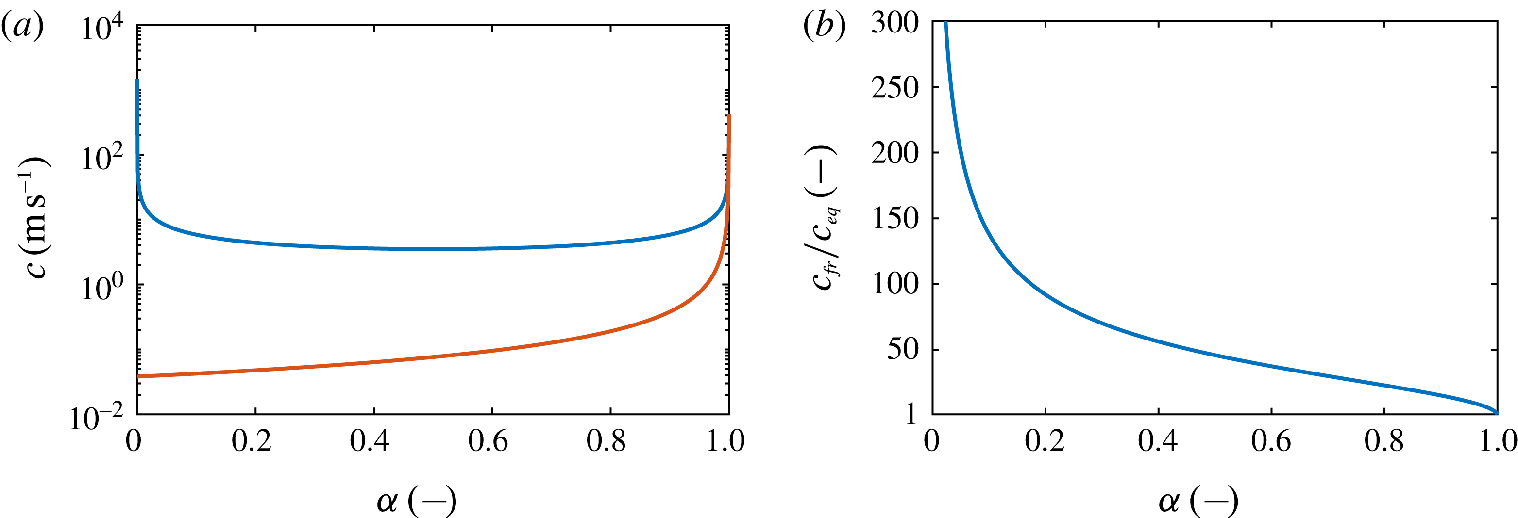
, a functional dependence for the speed of sound in the mixture region is required. As discussed in appendix A, estimates for upper and lower bounds are given by the frozen and equilibrium speeds of sound,
 $c_{fr}$
, (A 1), and
 $c_{eq}$
, (A 2), respectively. As shown in appendix A, selection of
 $c_{fr}$
leads to an underestimation of the vapour production rate. Alternatively, an intermediate model between frozen and equilibrium speed of sound would require additional information, e.g. bubble size distributions, interfacial areas between liquid and vapour phases, or approximations for the degree of thermal exchange between the phases. However, reliable estimates for these parameters are not available. To avoid the need for further assumptions, we chose the equilibrium speed of sound
 $c_{eq}$
for integrating (2.12).
The
 $\hat{p}$
–
 $\hat{v}$
phase diagram for the two-phase system of water and water vapour, including the barotropic equation of state
 $\hat{p}=\hat{p}(\hat{\unicode[STIX]{x1D70C}})$
(——, red). The lines denote the saturation lines of liquid and vapour
 $p_{l,sat}$
and
 $p_{v,sat}$
(– –), the saturation pressure
 $p_{sat}(T_{ref})$
(— - —) and the triple line
 $p_{triple}(T_{ref})$
(- - - -) at the barotropic reference temperature
 $T_{ref}$
.

The resulting barotropic equation of state
 $\hat{p}(\hat{\unicode[STIX]{x1D70C}})$
is depicted in figure 1 in the
 $\hat{p}$
–
 $\hat{v}$
phase diagram, with
 $\hat{v}=1/\hat{\unicode[STIX]{x1D70C}}$
denoting the specific volume. In this barotropic model, the evaporation rate is directly linked to the mixture speed of sound. As discussed in appendix A, lower values of
 $c$
are associated with stronger vapour production. It is to be noted, however, that complete evaporation, i.e. pure vapour (
 $\unicode[STIX]{x1D6FC}=1$
), cannot be reached in this model. As indicated in figure 1, the assumed isentropic phase change leads for
 $\unicode[STIX]{x1D6FC}\rightarrow 1$
to a crossing of the triple line at the reference temperature
 $p_{triple}(T_{ref})$
; see also the discussion of Mihatsch et al. (Reference Mihatsch, Schmidt and Adams2015). Hence, the triple line represents a constraint of the physical model, where the thermodynamic closures become invalid. The maximum admissible amount of the vapour void fraction is
 $\unicode[STIX]{x1D6FC}=99.984\,\%$
. Due to the low characteristic velocities in the present configuration, this value is, however, not reached in the computations.
2.4 Numerical approach
The numerical method is described in detail by Schnerr et al. (Reference Schnerr, Sezal and Schmidt2008) and Mihatsch et al. (Reference Mihatsch, Schmidt and Adams2015). An in-depth analysis is further given by Egerer et al. (Reference Egerer, Schmidt, Hickel and Adams2016). We thus only briefly summarise the main components here. The numerical method is a semi-discrete finite volume method, where the conservative form of the barotropic Euler equations is discretised in space using body-fitted block-structured hexahedral grids. Mass and momentum fluxes are approximated by numerical flux functions including a low-Mach consistent advection scheme; see Schmidt (Reference Schmidt2015). An upwind-biased reconstruction of the density is applied, together with a second-order central approximation for the interface pressure. For the reconstruction of the velocity, the total variation diminishing (TVD) limiter of Koren (Reference Koren1993) is applied, which is formally third-order accurate in smooth regions. In order to resolve all time scales of cavitating flow including shock-wave dynamics, explicit time integration is performed using a second-order four-step low-storage Runge–Kutta method. A constant Courant–Friedrichs–Lewy (CFL) number of
 $\mathit{CFL}=1.4$
is selected for all presented computations. The solver is fully parallelised using Message Passing Interface (MPI) directives and static load balancing is performed with the Metis graph partitioner; see Karypis & Kumar (Reference Karypis and Kumar1998).
In order to cope with numerical model uncertainty, the following measures are taken. First, with preparatory studies discussed in appendix B, the influence of the thermodynamic model is assessed. It is found that the high specific heat capacity of the liquid medium causes only minor temperature fluctuations. Hence, the temperature dependence of fluid properties is negligible. The present case is further characterised by a low convective flow velocity. The condensation shocks that occur and the associated entropy increases are thus weak. Moreover, baroclinic vorticity production is negligible for the dynamics of the considered system. We conclude that the influence of the thermodynamic model is insignificant. Second, the spatial resolution is investigated with a grid sensitivity study discussed in appendix E. Regarding the operating point and the associated global dynamics of the system, the presented analysis confirms grid convergence on the finest mesh
 $\mathit{lvl}_{2}$
. Third, the uncertainty originating from the numerical reconstruction scheme is investigated by repeating the simulations for the same configuration and operating point using an alternative numerical scheme based on the work of Egerer et al. (Reference Egerer, Schmidt, Hickel and Adams2016). In smooth regions of the flow, this method employs a linear fourth-order centred scheme for the velocity and pressure, while the density is reconstructed using the minmod limiter. At flow discontinuities, which are detected via a sensor functional, as discussed by Egerer et al. (Reference Egerer, Schmidt, Hickel and Adams2016), the upwind-biased reconstruction scheme of the present study is used. The spatial reconstruction of this method thus is of higher order in the bulk. Still, identical results, e.g. regarding the global cavity dynamics, are obtained, justifying the use of the present upwind-biased scheme. Fourth, uncertainty can also originate from the discretisation of the tunnel geometry. However, as physical viscosity is neglected and thus slip wall boundary conditions can be applied, no wall resolution is necessary. We assume that the manufacturing uncertainty is sufficiently low that it lies well within the first layer of computational cells adjacent to the tunnel walls. An exception might be the shape of the wedge apex, where a finite radius can influence the overall amount of cavitation through a modification of the local suction peak. However, no information on the actual geometry is available to us. We thus resort to modelling the apex as a sharp corner.
For all conclusions presented in the following, the inherent chaotic nature of the system has to be taken into account. This results in a lack of repeatability of the shedding process and noticeable cycle-to-cycle variations. This was already found by Ganesh et al. (Reference Ganesh, Mäkiharju and Ceccio2016) and needs to be considered when comparing numerical and experimental results. The simulations are thus sampled for an extended amount of time, in order to incorporate as many cycles as possible, while keeping the required wall-clock time for the computations at an acceptable level. For the time averages of numerical probes and the time-averaged flow field, the statistics on the finest grid cover 30 cycles, while 27 cycles are considered for investigating coherent structures and the attached cavity sheet length. Furthermore, the compressible approach exhibits transient acoustic waves developing from the simulation start-up. The presented statistical data are collected only after a sufficiently long start-up phase, so that all initial disturbances have decayed. This is determined by monitoring transient quantities, such as the mass flux through the outlet plane, the pressure and velocity at the upstream station 1 or the integral vapour volume within the entire computational domain.
3 Problem description
3.1 Experimental set-up
We reproduce the experimental work of Ganesh et al. (Reference Ganesh, Mäkiharju and Ceccio2016). A schematic of the experimental set-up is shown in figure 2. The test section, figure 2(a), possesses a quadratic cross-section of
 $76.2~\text{mm}\times 76.2~\text{mm}$
, with
 $h_{ch}=76.2~\text{mm}$
denoting the channel height. A quasi-two-dimensional wedge profile, shown in detail in figure 2(b), with a contraction angle of
 $\unicode[STIX]{x1D711}_{1}=22.1^{\circ }$
, a diffuser angle of
 $\unicode[STIX]{x1D711}_{2}=8.13^{\circ }$
and a height of
 $h_{w}=25.4~\text{mm}$
, is mounted on the bottom wall of the test section. The origin of the coordinate system coincides with the location of the wedge apex at mid-span. The
 $x$
-,
 $y$
- and
 $z$
-directions denote the streamwise, transverse and spanwise directions respectively. In the following, the test-section walls in the lower/upper transverse direction are denoted as bottom/top walls and in the lower/upper spanwise direction as left/right side- or lateral walls. The directions parallel and normal to the downstream face of the wedge are denoted by
 $s$
and
 $n$
respectively, as indicated in figure 2(b).
The test section is embedded into a circular feeding line with a diameter of
 $244.4~\text{mm}$
. At
 $464.4~\text{mm}$
upstream of the wedge apex, a double contraction connects the test section to the feeding line. Across this contraction, the cross-section changes from circular through an octagonal section to quadratic, as indicated in figure 2(a). At
 $571.5~\text{mm}$
downstream of the wedge apex, a mount discontinuously connects the test section back to the feeding line, with an additional variation in cross-section shape through an octagonal section.
Optical access to the region of the wedge is provided from the top and either side of the test section. Positions
 $1$
and
 $2$
in figure 2(a) indicate the locations of static pressure transducers
 $P_{1}$
and
 $P_{2}$
, which are utilised to specify the operating point in the experiment. In addition, as shown in figure 2(b), the pressure above the wedge is measured in the experiments by using the static pressure transducers
 $P_{A}$
and
 $P_{D}$
. These are located below the wedge surface, and connected to a circular opening of diameter
 $0.8~\text{mm}$
at mid-span of the wedge surface; see Ganesh et al. (Reference Ganesh, Mäkiharju and Ceccio2016). This locally modifies the geometry of the wedge surface in the experiments at mid-span, potentially acting as a nucleation site for cavitation. However, due to the small physical dimensions of the probe, the effect on the overall system behaviour is expected to be negligible.
Experimental set-up, showing (a) the test section and (b) the convergent–divergent wedge. The sketches include the coordinate systems
 $(x-y)$
and
 $(s-n)$
, and the locations
 $1$
,
 $2$
,
 $P_{A}$
and
 $P_{D}$
employed for numerical probes.

3.2 Computational domain and grid
The computational domain, depicted in figure 3, reproduces the nominal experimental set-up. We consider a feeding line with a length of approximately
 $1~\text{m}$
ahead of the double contraction. The double contraction, the test section and the rear mount back to the feeding line are identical to the experimental set-up, including all changes in cross-section shape and size. Approximately
 $1~\text{m}$
downstream of the test section, the feeding line connects to an additional large circular tube with a diameter of
 $800~\text{mm}$
and a length of
 $500~\text{mm}$
. Although this tube is not part of the experimental facility, it allows for improved specification of the boundary conditions. In the experiment, pressure waves originating from, e.g., cavity collapse events in the vicinity of the wedge are able to travel through the whole facility, where a damping due to large increases in cross-sections occurs. The additional tube in the computational set-up causes a comparable effect. However, adjustment of the pressure at the end of the additional tube is required in order to recover the experimentally measured pressure at position 2 in the test section.
Side view (
 $x{-}y$
plane) of the entire numerical domain, including the duct up- and downstream of the test section and the large diffuser near the outlet boundary.

Numerical mesh, showing the
 $\mathit{lvl}_{1}$
grid in the region of the test section. (a) Side view on the
 $x{-}y$
plane. (b) Variation of cross-sections
 $A{-}A$
to
 $E{-}E$
in the
 $y{-}z$
plane.

Three grid levels, denoted as
 $\mathit{lvl}_{0}$
,
 $\mathit{lvl}_{1}$
and
 $\mathit{lvl}_{2}$
, are created; see table 4 for details. All grids are body-fitted block-structured hexahedral grids. The finest grid level comprises 24 million elements for the complete domain, with 17.5 million cells located within the test section excluding the double contraction. In the vicinity of the wedge, as visualised in figure 4, the grid is aligned parallel to the wedge surface in order to increase the spatial resolution of the sheet cavity. Cubic control volumes with a constant cell edge length of up to
 $n=30~\text{mm}$
above the wedge are utilised in this region. The minimum grid spacing on the finest grid level is
 $l_{s}=l_{n}=l_{z}=0.5~\text{mm}$
.
The parameters of the numerical grids employed.

3.3 Boundary conditions
At the inlet plane of the upstream feeding line, a homogeneous inflow velocity
 $u_{0}$
is specified, while an asymptotic boundary condition on the static outlet pressure
 $p_{3}$
is utilised at the outlet plane of the large downstream diffuser. All walls are modelled as slip walls as we neglect viscous effects.
Ganesh et al. (Reference Ganesh, Mäkiharju and Ceccio2016) specified the operating point of the experiment by measuring the static pressure at points
 $1$
and
 $2$
in figure 2. The bulk velocity
 $u_{1}$
at position
 $1$
was derived by Ganesh et al. (Reference Ganesh, Mäkiharju and Ceccio2016) by measuring the pressure drop between two upstream locations and their corresponding area ratios, and then applying Bernoulli’s law. In the experiments,
 $p_{1}=63~\text{kPa}$
, giving an upstream cavitation number of
 $\unicode[STIX]{x1D70E}_{1}=(p_{1}-p_{vap})/(\unicode[STIX]{x1D70C}_{ref}u_{1}^{2}/2)=1.95$
. Ganesh et al. (Reference Ganesh, Mäkiharju and Ceccio2016) stated an uncertainty of
 $\pm 0.1~\text{m}~\text{s}^{-1}$
for the computed upstream velocity and
 $\pm 2~\text{kPa}$
for the pressure measurements. This leads to an overall uncertainty in the cavitation number of
 $\pm 0.11$
.
In order to reproduce the experimental operation point in our computations, both
 $u_{0}$
and
 $p_{3}$
are adjusted iteratively, until the velocity
 $u_{1}=7.9~\text{m}~\text{s}^{-1}$
at position
 $1$
and the static pressure
 $p_{2}=55~\text{kPa}$
at position
 $2$
match with the experimental values. The matching is performed on grid
 $\mathit{lvl}_{0}$
. For the subsequent levels
 $\mathit{lvl}_{1}$
and
 $\mathit{lvl}_{2}$
, identical boundary conditions are used. Since the pressure
 $p_{2}$
is controlled with the downstream boundary condition, the pressure
 $p_{1}$
depends on the pressure drop in the test section. It is hence part of the solution. Consequently, the upstream cavitation number
 $\unicode[STIX]{x1D70E}_{1}$
in the simulation cannot be independently prescribed. A definition of the operating point in the computations through the imposed boundary conditions motivates the cavitation number
 $\unicode[STIX]{x1D70E}_{2}=(p_{2}-p_{vap})/(\unicode[STIX]{x1D70C}_{ref}u_{1}^{2}/2)$
. As will be shown subsequently, we find
 $\unicode[STIX]{x1D70E}_{2}=1.7$
, which is a perfect match between simulation and experiment.
3.4 The simulations conducted
With preparatory studies, discussed in appendix B, the influence of the thermodynamic model is assessed. It is found that, first, the high specific heat capacity of the liquid medium limits the amplitude of temperature fluctuations. The temperature dependence of fluid properties is hence negligible. Second, the present case is characterised by a low convective flow velocity. The condensation shocks that occur and the associated entropy increases are thus weak. Third, by analysing the budgets of the vorticity-transport equation (VTE), i.e. vortex stretching, compressible dilatation and baroclinic torque, we find that the latter is negligible for the dynamics of the considered system. We conclude that the influence of the thermodynamic model is insignificant. The subsequent discussion hence focuses on results obtained with the barotropic model, due to its considerably lower computational cost.
Overview of simulations conducted with the barotropic model.

Flow properties up- and downstream of the test section; comparison between numerical results on grids
 $\mathit{lvl}_{0}$
,
 $\mathit{lvl}_{1}$
and
 $\mathit{lvl}_{2}$
, and the experimental reference.

A grid sequencing method is employed, consisting of consecutive computations with increasing resolution in space and time. Statistically converged solutions from a coarse grid are thereby interpolated to the next finer grid. This significantly shortens transients on the finer grid levels and thus reduces the computational cost. Three grid levels, denoted as
 $\mathit{lvl}_{0}$
,
 $\mathit{lvl}_{1}$
and
 $\mathit{lvl}_{2}$
, are employed. Table 5 summarises the simulations conducted, showing the average time step, the interval used for statistical sampling and the total run time in terms of physical as well as computational time. Transients associated with simulation start-up and after interpolation are excluded from this evaluation.
4 Results
4.1 Operating point
The agreement with the experimental operating point is assessed by evaluating the temporal mean, denoted by an overbar,
 $\overline{\bullet }$
, of quantities recorded at probing locations
 $1$
and
 $2$
, and by comparison of the velocity profile upstream of the wedge.
Table 6 shows the obtained mean velocity
 $\overline{u}_{1}$
and pressures
 $\overline{p}_{1}$
,
 $\overline{p}_{2}$
. Additionally, the mean cavitation numbers
 $\overline{\unicode[STIX]{x1D70E}}_{1}$
and
 $\overline{\unicode[STIX]{x1D70E}}_{2}$
are given. The quantities
 $\overline{u}_{1}$
and
 $\overline{p}_{2}$
, controlled with the boundary conditions, match the experimental references and vary only little for the different grid levels. Correspondingly, an almost exact agreement is obtained for the cavitation number
 $\overline{\unicode[STIX]{x1D70E}}_{2}$
. In contrast, the mean upstream pressure
 $\overline{p}_{1}$
is consistently higher in the simulations for all three grid levels. As already discussed, the upstream pressure, and thus also the upstream cavitation number, is part of the solution. Compared with the experiments,
 $\overline{p}_{1}$
and
 $\overline{\unicode[STIX]{x1D70E}}_{1}$
are larger by approximately 10 %, indicating that the pressure loss
 $\unicode[STIX]{x0394}p=p_{1}-p_{2}$
in the test section is higher in the simulation.
Two factors contribute to the higher pressure drop in the simulation. First, vapour structures, causing a blockage effect, induce additional pressure losses. For the present case and operating point, the extent of vapour structures intermittently reaches almost the size of the channel cross-section. The pressure losses associated with cavitation thus exceed the losses due to viscous effects within the test section. As discussed in § 4.6, the mean amount of vapour produced is larger in the simulations compared with the experiments, thus causing a larger contribution to the pressure drop in the simulation. Second, the pressure on the upstream shoulder of the wedge has a large influence on the overall pressure drop as well. See appendix C for an analytical model that can be used to explain the observed differences between the pressure drop in the simulations and the experimental references. These are the primary reasons for the larger pressure drop
 $\unicode[STIX]{x0394}p$
and thus the deviations found in
 $\overline{p}_{1}$
and
 $\overline{\unicode[STIX]{x1D70E}}_{1}$
. In view of the uncertainty in the measurements, the agreement with the experimental operating point can still be considered to be satisfactory. The analytical model derived in appendix C shows that the present configuration generates a pressure loss, even under inviscid assumptions. It thus is analogous to the generation of wave drag in inviscid supersonic flow. Here, it is caused solely by the presence of two-phase flow, which prevents a pressure recovery on the back side of the wedge.
Due to the inviscid assumption, viscous effects, such as boundary layers or corner vortices within the channel, are not captured by the numerical simulation. This could potentially alter the effective inflow conditions to the cavitating region. The velocity profile upstream of the wedge is analysed in appendix D. It is found that upstream of the wedge, the near-wall viscous layer spans less than 2 % of the channel height. Due to the subsequent acceleration of the flow on the convergent part of the wedge, the boundary layer is expected to be even thinner when reaching the sharp wedge apex. From this investigation, it is concluded that the incoming boundary layer does not have a significant influence on the sheet cavity, and that the assumptions of inviscid flow and slip boundary conditions in the two-phase computations are sound.
With only small changes between the quantities
 $\overline{u}_{1}$
,
 $\overline{p}_{1}$
and
 $\overline{p}_{2}$
obtained on grids
 $\mathit{lvl}_{1}$
and
 $\mathit{lvl}_{2}$
, table 6 already gives an indication that the numerical results on the finest level can be considered as grid-converged. This is confirmed by a detailed analysis of grid convergence, provided in appendix E. The following discussion hence focuses on results obtained on the finest grid.
4.2 Instantaneous flow topology
Figure 5 compares instantaneous simulation results with snapshots from experimental high-speed videos in top view. For a visualisation of the numerical results, isosurfaces of the 10 % void fraction are chosen. Furthermore, instantaneous vortical structures are shown with isosurfaces of
 $\unicode[STIX]{x1D706}_{2}=-2\times 10^{6}~\text{s}^{-2}$
, coloured by the axial vorticity
 $\unicode[STIX]{x1D714}_{x}$
. Here,
 $\unicode[STIX]{x1D706}_{2}$
denotes the second eigenvalue of
 $\unicode[STIX]{x1D64E}^{2}+\unicode[STIX]{x1D734}^{2}$
, where
 $\unicode[STIX]{x1D64E}$
and
 $\unicode[STIX]{x1D734}$
are the symmetric and asymmetric parts of the velocity gradient tensor
 $\boldsymbol{\unicode[STIX]{x1D6FB}}\unicode[STIX]{x1D66A}$
respectively. Dash-dotted lines indicate the location of the apex
 $(x=0)$
and rear edge (
 $x=x_{w}$
) of the wedge. For illustration of the shedding process, five representative time instants are selected in figure 5(a–e), exhibiting typical topological features and coherent flow structures. It is unknown which precise value of
 $\unicode[STIX]{x1D6FC}$
corresponds best to a visual examination of cavitation from experiments. Furthermore, it is unclear whether a single value actually exists, considering the broad range of cavitation topologies (bubble cavitation, sheet cavitation, cloud cavitation) that can be covered with the homogeneous mixture approach. We choose the value of
 $\unicode[STIX]{x1D6FC}=0.1$
for visualising the numerical results. A further aspect for such a juxtaposition is the highly transient nature of the flow and the lack of repeatability of the shedding process. Due to the inherent chaotic nature of cavitating flow, this equally affects the simulation and the experiments. We thus do not expect to find identical flow structures for any two arbitrarily selected time instants. However, for a qualitative assessment of flow structures, the presented analysis is suitable.
Illustration of a typical shedding cycle (top view); comparison between experiment (left, from direct communication with H. Ganesh) and simulation on the
 $\mathit{lvl}_{2}$
grid (right). The numerical results show vapour structures with the isosurface of
 $\unicode[STIX]{x1D6FC}=0.1$
(grey) and vortical structures with the isosurface of
 $\unicode[STIX]{x1D706}_{2}=-2\times 10^{6}~\text{s}^{-2}$
, coloured by the axial vorticity
 $\unicode[STIX]{x1D714}_{x}$
. The white boxes indicate coherent flow structures, and the dash-dotted lines denote the wedge apex (
 $x=0$
) and the wedge rear point (
 $x=x_{w}$
).

Figure 5(a) shows the time instant of maximum attached sheet cavity length. The sheet, curved towards both sidewalls, attains its largest streamwise extent at mid-span. The experimental picture shows small-scale streamwise-oriented cavitating vortices (‘streamers’; see Laberteaux & Ceccio Reference Laberteaux and Ceccio2001) trailing from the attached sheet at mid-span. Furthermore, cavitating vortices are situated along both sidewalls. A streamwise-oriented vortex is located close to the left sidewall and is connected to the sheet. Another vortex, oriented normal to the bottom wall and propagating downstream, is located close to the right sidewall. The simulations equally exhibit these flow structures. Side views provided by Ganesh et al. (Reference Ganesh, Mäkiharju and Ceccio2016) show that the streamwise-oriented vortices in the vicinity of the lateral walls are typically detached from the bottom wall. They are different from corner vortices found in turbulent channel flow. Rather, they are characteristic features of the cavitating flow, similar to ‘streamers’, resulting from the non-uniform distribution of circulation in the spanwise direction. The latter originates from the non-planar and variable-strength condensation shock front, causing the downstream advection of vortex lines. Furthermore, the isosurfaces show perturbations of the attached sheet along the sidewalls, developing downstream of the apex, which are also found in the experimental picture.
Figure 5(b) depicts the situation of a condensation shock propagating through the attached sheet towards the wedge apex. As indicated by the dashed line, the progression of the shock is faster at mid-span, while it is slightly slower close to the sidewalls. Simultaneously, a large cavitating horseshoe vortex develops at the downstream part of the vapour structure. Just upstream of the horseshoe vortex, a so-called crescent-shaped region is found, a typical flow phenomenon of cavitating flow; see, e.g., Reisman et al. (Reference Reisman, Wang and Brennen1998). The simulations also predict the occurrence of the condensation shock phenomenon, with a non-uniform rate of progression across the spanwise direction. Likewise, large cavitating horseshoe vortices, as well as crescent-shaped regions, can be found.
Figure 5(c) depicts the instant when the condensation front touches the wedge apex. For most shedding cycles, this does not occur simultaneously across the complete span. Instead, the shock reaches the apex first close to mid-span, while it lags slightly behind near the lateral walls. A similar behaviour is found in the simulation. When the shock reaches the apex, a detached cloud is generated, concentrating strong vorticity along the spanwise direction. Typically, ‘streamers’, as shown by the experimental picture, or horseshoe vortices, as depicted in the numerical visualisation, develop at the trailing part of the cloud.
Figure 5(d) shows the situation just after the detachment along the entire spanwise direction, and development of a fully separated cloud further downstream. The region just downstream of the apex, denoted as ‘leading-edge’ separation in the figure, is characterised by complex flow patterns. Cavitating vortices are mainly oriented along the spanwise direction, partially forming horseshoe-type structures. Streamwise-oriented vortices connect these patches of cavitation. The flow topology predicted by the simulation resembles the experimental picture. The formation of separated flow at the apex differs from viscous flow separation. Comparable to the detachment caused by a re-entrant jet, it is induced by the reverse flow following behind the upstream-propagating condensation front, which reaches the apex.
Finally, at the instant shown in figure 5(e), the separated cloud is convected further downstream, while a new cavity sheet develops. Typical for this situation is the observation of large cavitating vortices wrapping around the cloud, oriented primarily in the streamwise direction. The simulation exhibits comparable structures.
On comparing experimental and numerical panels (a–e), it can be observed that the simulation exhibits slightly less small-scale cavitation. Yet, the
 $\unicode[STIX]{x1D706}_{2}$
-criterion illustrates the existence of complex vortical structures. For example, smaller streamwise-oriented vortices can be found at the downstream part of the cloud as well as concentrated close to the tunnel sidewalls. This indicates that the pressure drop in these vortex cores is not sufficient for cavitation to occur. Resolution of the vortex cavitation within these small-scale structures would require a much finer numerical grid. However, the larger cavitating structures (e.g. horseshoe cavitation on a variety of length scales, crescent-shaped regions, streamers, vortices along the sidewalls in the streamwise direction as well as normal to the bottom wall) are predicted in close agreement with the experiments. From this qualitative comparison, it can be concluded that the selected numerical model is able to capture the primary features present in the cavitating flow of sheet-to-cloud transition.
The shedding process can also be visualised with the spanwise average, denoted by
 $\langle \,\bullet \,\rangle _{z}$
in the following. For this purpose, figure 6 shows a series of six consecutive time instants in the form of the instantaneous spanwise-averaged void fraction
 $\langle \unicode[STIX]{x1D6FC}\rangle _{z}$
, the streamwise velocity
 $\langle u\rangle _{z}$
and the pressure
 $\langle p\rangle _{z}$
in the vicinity of the wedge. The plots of velocity and pressure include isocontours of
 $\langle \unicode[STIX]{x1D6FC}\rangle _{z}$
to relate these fields to the occurrence of cavitation.
The spanwise-averaged instantaneous flow field during a shock-dominated shedding cycle for six consecutive time instants; numerical prediction on the
 $\mathit{lvl}_{2}$
grid. Comparison between (a) the void fraction
 $\langle \unicode[STIX]{x1D6FC}\rangle _{z}$
, (b) the streamwise velocity
 $\langle u\rangle _{z}$
and (c) the pressure
 $\langle p\rangle _{z}$
. Isocontours of
 $\langle \unicode[STIX]{x1D6FC}\rangle _{z}$
are superimposed on
 $\langle u\rangle _{z}$
and
 $\langle p\rangle _{z}$
.

The first instant,
 $t=t_{0}$
, depicts the instant when the attached sheet reaches its maximum length in the streamwise direction; here,
 $s_{L}\approx 100~\text{mm}$
. The spanwise-averaged void fraction attains values close to
 $\langle \unicode[STIX]{x1D6FC}\rangle _{z}\approx 0.8$
. Within the sheet, the local flow velocity is small and is directed downstream, while the spanwise-averaged pressure attains values close to the vapour pressure. Shortly thereafter, a condensation shock forms at the rear part of the attached sheet. In the subsequent time instants,
 $t=t_{0}+6~\text{ms}$
and
 $t=t_{0}+12~\text{ms}$
, the condensation shock propagates upstream through the sheet. Simultaneously, the spanwise-averaged void fraction in the attached part of the sheet increases, reaching values of
 $\langle \unicode[STIX]{x1D6FC}\rangle _{z}\approx 0.9$
. The condensation front spans almost the complete height of the attached sheet and causes condensation. Across the shock, the direction of flow is reversed and the static pressure increases. A shear layer forms between the free-stream and the upstream-directed flow behind the shock, exhibiting classical Kelvin–Helmholtz instabilities. Within the low-pressure vortex cores, evaporation takes place. This leads to the formation of new cavity structures behind the shock, subsequently rolling up into a cloud. Across the condensation front, the more dense liquid displaces the lighter mixture region within the sheet. As a consequence, Rayleigh–Taylor instabilities develop along the interface. In addition to the non-uniform rate of progression noted above, the resulting perturbations of the interface contribute to the fact that it does not appear as a sharp front in the spanwise average. At
 $t=t_{0}+17~\text{ms}$
, the shock touches the wedge apex. Again, caused by variations in the spanwise direction, this does not happen uniformly across the wedge, and the spanwise-averaged void fraction is non-zero close to the apex for this instant. Simultaneously, the downstream cloud is continuously fed by the shear layer. Due to the upstream-directed flow following behind the shock front, the cloud is not yet detached. Detachment across the complete spanwise direction is shown at the next instant,
 $t=t_{0}+21~\text{ms}$
. The upstream-directed flow breaks down, and the cloud separates and starts to propagate downstream. With the cloud being convected downstream, the growth of a new sheet is initiated, as shown at the last instant,
 $t=t_{0}+27~\text{ms}$
.
For a total of 27 shedding cycles, the maximum attached sheet length
 $s_{L}$
is determined from the spanwise-averaged void fraction. The average yields a mean attached sheet length of
 $\overline{s}_{L}=108.4~\text{mm}$
. A measure for the cycle-to-cycle variation is given by the standard deviation of
 $\overline{s}_{L}$
, which amounts to
 $\pm 13~\text{mm}$
.
4.3 Temporal evolution of the shedding process
The shedding process across multiple cycles can be further analysed by recording the temporal evolution of the spanwise-averaged flow on a plane at a normal distance
 $n=n_{p}$
parallel to the wedge surface. Choosing
 $n_{p}=5.2~\text{mm}$
, figure 7 shows the thus obtained variation in time for the void fraction
 $\left.\langle \unicode[STIX]{x1D6FC}\rangle _{z}\right|_{n_{p}}$
and axial velocity
 $\left.\langle u\rangle _{z}\right|_{n_{p}}$
, plotted along the
 $s$
-direction for a time span of
 $1~\text{s}$
.
The time evolution of the shedding process over a period of
 $1~\text{s}$
; numerical prediction on the
 $\mathit{lvl}_{2}$
grid. Spanwise-averaged quantities are extracted from a wedge-parallel plane at a normal distance of
 $n=n_{p}=5.2~\text{mm}$
and plotted along
 $s$
. Comparison of (a) the void fraction
 $\left.\langle \unicode[STIX]{x1D6FC}\rangle _{z}\right|_{n_{p}}$
and (b) the axial velocity component
 $\left.\langle u\rangle _{z}\right|_{n_{p}}$
. The slopes indicated by black lines denote processes of cavity growth (
 $\overline{u}_{growth}=5.5~\text{m}~\text{s}^{-1}$
) and cavity collapse (
 $\overline{u}_{shock}=-4.5~\text{m}~\text{s}^{-1}$
).

Individual shedding cycles can be identified by the triangular shape in the plot of
 $\left.\langle \unicode[STIX]{x1D6FC}\rangle _{z}\right|_{n_{p}}$
. The black solid lines exemplarily highlight several cycles. Positive slopes denote processes of cavity growth, i.e. the formation of a new attached sheet. For most cycles, typical void fractions in the attached sheet exceed 70 %, with a tendency to increase during the growth process and towards the wedge apex, as already noted above. In general, the flow is directed downstream within the sheets and the velocity magnitude is small. After reaching a maximum sheet length, a new process of cavity collapse is initiated, indicated by negative slopes in figure 7. Due to the restriction to the plane
 $n=n_{p}$
, the structures observed here are slightly shorter than the maximum attached sheet length
 $\overline{s}_{L}$
computed above. The majority of collapse processes are associated with the occurrence of a condensation shock. Behind the shock, the flow is directed upstream and the magnitude of the flow velocity is significantly increased. In most cycles, the void fraction drops across the shock to values close to zero, as expected. For some cycles, however, non-zero vapour content is present just downstream of the condensation shock. On one hand, this is associated with the cavitating shear layer following immediately behind the shock. On the other hand, the front propagation velocity may be inhomogeneous along the spanwise direction, as mentioned above. During the collapse process, the cloud, still being connected to the sheet, moves downstream only moderately. For most cycles it does not pass beyond
 $s\approx 150~\text{mm}$
. At the time instant when the shock touches the apex, the cloud completely separates and is convected further downstream.
The slopes in figure 7 can be used to estimate the characteristic velocities for the cavity growth and collapse processes. The cavity growth velocity, on average
 $\overline{u}_{growth}=5.5~\text{m}~\text{s}^{-1}$
, is approximately constant during a given shedding cycle. The velocity of cavity collapse, corresponding to the propagation velocity of the condensation shock front
 $\overline{u}_{shock}$
, is found to be
 $\overline{u}_{shock}\approx -4.5~\text{m}~\text{s}^{-1}$
on average. The front undergoes a slight acceleration when it approaches the wedge apex. Figure 8 compares the value of
 $\overline{u}_{shock}$
obtained numerically with experimental measurements for upstream cavitation numbers in the range
 $1.88\leqslant \unicode[STIX]{x1D70E}_{1}\leqslant 2.19$
. The computed value for the front propagation velocity is in close agreement with the experimentally reported values.
Average propagation velocity of condensation shocks
 $\overline{u}_{shock}$
. Comparison between simulation (


The acceleration of the condensation shock towards the wedge apex is caused by the fact that the void fraction in the sheet close to the apex increases during the process of cavity collapse, as seen from figures 6 and 7. This is in agreement with the findings of Brennen (Reference Brennen1995), who, neglecting bubble dynamics, surface tension and phase change, derived the following equation for the front propagation velocity relative to the upstream fluid
 $u_{shock,rel}$
in a bubbly flow:
 $$\begin{eqnarray}\displaystyle & \displaystyle u_{shock,rel}^{2}=\frac{p_{2}-p_{1}}{\unicode[STIX]{x1D70C}_{L}}\cdot \frac{1-\unicode[STIX]{x1D6FC}_{2}}{(1-\unicode[STIX]{x1D6FC}_{1})(\unicode[STIX]{x1D6FC}_{1}-\unicode[STIX]{x1D6FC}_{2})}. & \displaystyle\end{eqnarray}$$
States upstream and downstream of the shock are denoted by subscripts ‘1’ and ‘2’ respectively. Assuming the pressure drop
 $p_{2}-p_{1}$
to be almost constant across the front,
 $u_{shock,rel}$
increases when
 $\unicode[STIX]{x1D6FC}_{1}\rightarrow 1$
. As seen from figure 7, the velocity of the flow upstream of the front also remains approximately constant. Thus, the absolute velocity of the condensation front,
 $u_{shock}$
, increases as well.
Figure 7 shows that the predicted shedding process does not undergo perfect repeatability. This is documented for the current configuration by Ganesh et al. (Reference Ganesh, Mäkiharju and Ceccio2016). It is also a general feature of sheet-to-cloud shedding, as, e.g., described by Reisman et al. (Reference Reisman, Wang and Brennen1998). For the present case, irregular processes of cavity growth in between two main sheddings can be found in figure 7, e.g. around
 $t=0.08~\text{s}$
,
 $t=0.61~\text{s}$
,
 $t=0.79~\text{s}$
and
 $t=0.82~\text{s}$
. These are associated with the occurrence of a classical re-entrant jet instability. According to Ganesh et al. (Reference Ganesh, Mäkiharju and Ceccio2016), this is more frequent at higher cavitation numbers. As reported by these authors, however, it can also appear for the chosen operating point. Furthermore, it is observed from the simulations that a large coherent collapse of a cloudy structure can prematurely stop the sheet before it reaches its ‘natural’ maximum sheet length, as dictated by the adverse pressure gradient. Thereby initiating a condensation front, this downstream cloud collapse depends, e.g., on the previous cycle, neighbouring cavity structures, etc. Furthermore, a cloud collapse does not necessarily occur at mid-span. This can initiate sheet retraction primarily at one side, while the opposite side lags behind. This in turn affects the next cycle and may promote variations in the spanwise direction. The entire shedding process thus is chaotic. This contributes to the cycle-to-cycle variations in figure 7, e.g. regarding the maximum void fraction reached in the sheets, the internal structures in the sheets and the attached sheet length. The visualisation in figure 7 exhibits a subharmonic behaviour at a frequency lower than the shedding frequency, which can, e.g., be seen in the maximum vapour content in the sheets and the sheet length, which might also be a result of the abovementioned mechanism of premature sheet collapse. This is compared with the experiments in § 4.6.4.
4.4 Mean flow topology
The time- and spanwise-averaged flow field in the test section; numerical prediction on the
 $\mathit{lvl}_{2}$
grid. Comparison of (a) the pressure
 $\langle \overline{p}\rangle _{z}$
, (b) the axial velocity
 $\langle \overline{u}\rangle _{z}$
and (c) the void fraction
 $\langle \overline{\unicode[STIX]{x1D6FC}}\rangle _{z}$
. The direction of flow is indicated by streamlines; the red solid line indicates a region of reversed flow
 $\langle \overline{u}\rangle _{z}=0$
; the white dashed frame highlights the field of view for the experimental x-ray densitometry of Ganesh et al. (Reference Ganesh, Mäkiharju and Ceccio2016).

In order to analyse the time-averaged flow field in this section, the results obtained on the
 $\mathit{lvl}_{2}$
grid are sampled for a time span of
 $1.66~\text{s}$
, comprising approximately 30 shedding cycles. Figure 9 depicts the two-dimensional flow field obtained by averaging in time and the spanwise direction. The contour plots show the mean pressure
 $\langle \overline{p}\rangle _{z}$
, axial velocity
 $\langle \overline{u}\rangle _{z}$
and void fraction
 $\langle \overline{\unicode[STIX]{x1D6FC}}\rangle _{z}$
in the vicinity of the wedge. The direction of the mean flow is indicated by streamlines; a contour line of
 $\langle \overline{u}\rangle _{z}=0~\text{m}~\text{s}^{-1}$
highlights a region of reversed mean flow. Due to the convergent shape of the channel, the mean flow is accelerated above the wedge. Correspondingly, the local static pressure drops, reaching values close to the vapour pressure on the back side of the wedge. Accordingly, a contiguous region of cavitation is present in the temporal mean. Located above the back side of the wedge, it originates from the sharp wedge apex. A narrow region of reversed flow exists just above the wedge in the mean flow, spanning less than half of the cavity height.
The mean flow is not homogeneous in the spanwise direction. This is illustrated by figure 10, showing the time-averaged three-dimensional flow field. The mean cavitation pattern is visualised by an isosurface of the 20 % void fraction. Slices perpendicular to the spanwise direction show the local time-averaged void fraction
 $\overline{\unicode[STIX]{x1D6FC}}$
above the wedge, with a cutoff at
 $\overline{\unicode[STIX]{x1D6FC}}<0.1$
. On the bottom and left sidewalls of the channel, the contour of the mean velocity in the streamwise direction,
 $\overline{u}$
, is given. An isocontour of
 $\overline{u}=0~\text{m}~\text{s}^{-1}$
denotes a region of reversed flow present in the time-averaged flow field. Vortical structures are shown by isosurfaces of
 $\overline{Q}=1\times 10^{5}~\text{s}^{-2}$
, with
 $\overline{Q}$
denoting the time average of the instantaneous
 $Q$
-criterion,
 $Q=1/2(\Vert \unicode[STIX]{x1D64E}\Vert ^{2}-\Vert \unicode[STIX]{x1D734}\Vert ^{2})$
. The orientation of the vortices is given by colouring the isosurface by the local mean axial vorticity
 $\overline{\unicode[STIX]{x1D714}}_{x}$
. Despite the fact that the long time span of the temporal average contains many shedding cycles, fluctuations in the isosurface of the vapour volume fraction can be observed. However, these deviations can be regarded as small, and the statistics are considered as sufficiently converged.
The time-averaged flow field in the vicinity of the wedge; numerical prediction on the
 $\mathit{lvl}_{2}$
grid. Vapour structures are shown by isosurfaces of
 $\overline{\unicode[STIX]{x1D6FC}}=0.2$
and vortical structures by isosurfaces of
 $\overline{Q}=1\times 10^{5}~\text{s}^{-2}$
, coloured by the axial vorticity
 $\overline{\unicode[STIX]{x1D714}}_{x}$
. Contours of
 $\overline{\unicode[STIX]{x1D6FC}}$
are given in three slices perpendicular to the spanwise direction, with a cutoff at
 $\overline{\unicode[STIX]{x1D6FC}}<0.1$
. The tunnel walls show the contours of the axial velocity
 $\overline{u}$
. The red solid line (
 $\overline{u}=0$
) indicates a region of reversed flow.

The streamwise extent of the time-averaged vapour structure is largest at mid-span. Simultaneously, the region of reversed flow extends further downstream close to the sidewalls. Two counter-rotating vortices along the streamwise direction are present in the temporal mean. These vortices originate from the corner between the sidewalls and the bottom wall of the test section, just downstream of the contiguous mean vapour structure. They are inclined slightly away from the bottom wall and oriented such that fluid is transported along the lateral walls in the positive
 $y$
-direction, converging towards mid-span. This spanwise inhomogeneity of the time-averaged flow is caused by the presence of the sidewalls.
A direct verification of the three-dimensional mean flow structure with the experiments is not possible, as no corresponding data are available. However, it is in alignment with the observations made in the context of figure 5 above. All presented instantaneous images exhibit noticeable variations along the spanwise direction, e.g. the development of horseshoe vortices in the centre of the channel and vortices along the sidewalls, and show that the extent of the attached sheets is largest at mid-span. Thus, the presence of the sidewalls cannot be neglected in the simulations. We conclude that the global flow topology is correctly captured, even though slip boundary conditions due to the inviscid modelling are used in the present study.
4.5 Spectral analysis
In order to identify the dominant frequencies and their spatial distribution in the system, a spectral analysis for signals recorded within the entire test section is carried out. For this purpose, the local axial velocity component
 $u$
and pressure
 $p$
are recorded along the bottom wall of the test section by a total of 55 numerical probes. The probes are located at mid-span and distributed evenly in the streamwise direction with a spacing of
 $\unicode[STIX]{x0394}x\approx 11~\text{mm}$
between two consecutive probes. For the spectral analysis, Welch’s method is applied. The signals are sampled with a time resolution as given in table 5 and then linearly interpolated on a constant time step of
 $1\times 10^{-6}~\text{s}$
. The spectra are estimated using Hanning window segments with equal window length in the time domain of
 $0.2~\text{s}$
and
 $50\,\%$
overlap between subsequent segments.
Frequency spectra for the signals of (a) velocity
 $u$
and (b) pressure
 $p$
recorded by probes distributed within the test section along the bottom wall at mid-span. The dashed lines (– –) indicate the locations of the wedge apex (
 $x=0$
) and the rear point (
 $x=x_{w}$
), and the dash-dotted lines (— - —) indicate the mean of the maximum attached sheet length (
 $x=\overline{x}_{L}$
).
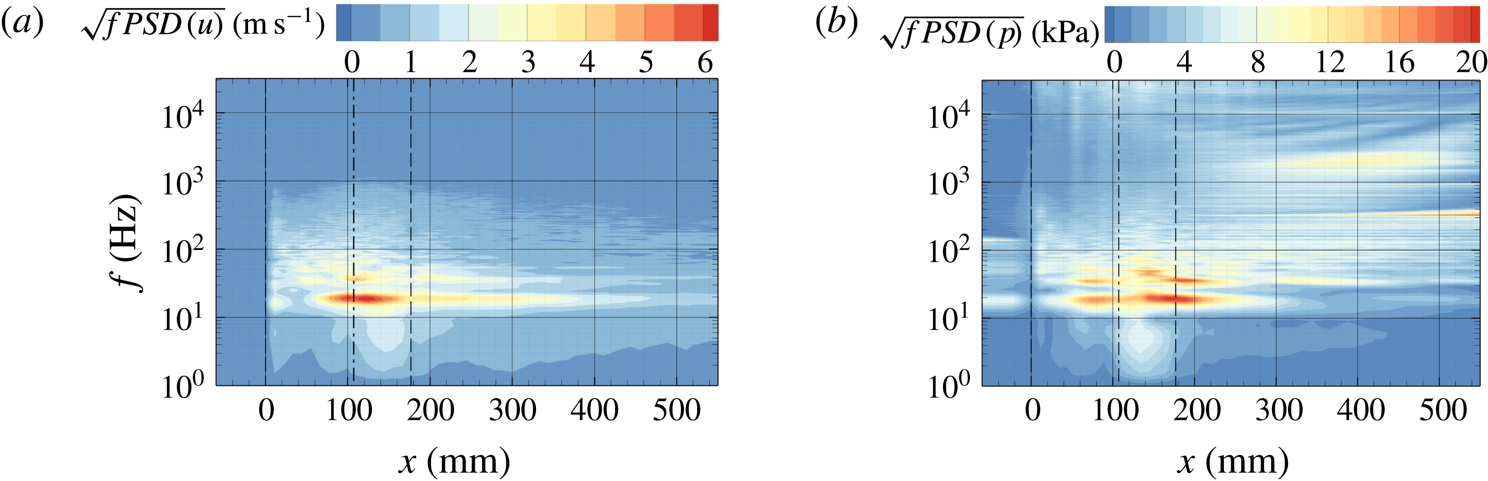
The time-averaged flow quantities used for non-dimensionalisation of the frequency spectra plotted in figure 11. Juxtaposition of (a) mean velocity
 $\overline{u}_{bottom}$
and (b) pressure
 $\overline{p}_{bottom}$
recorded at mid-span along the bottom wall. The dashed lines (– –) indicate the locations of the wedge apex (
 $x=0$
) and the rear point (
 $x=x_{w}$
), and the dash-dotted lines (— - —) indicate the mean of the maximum attached sheet length (
 $x=\overline{x}_{L}$
).

The frequency content is displayed in figure 11. The plots show the square root of the premultiplied power spectral density,
 $\sqrt{f\,PSD(\bullet )}$
, as a function of the streamwise position. The computed spectra for the axial velocity
 $u$
, figure 11(a), and the pressure
 $p$
, figure 11(b), can thus be interpreted as the RMS amplitude at a given frequency. A non-dimensional representation of the spectra is obtained using the local mean quantities for normalisation,
 $\sqrt{f\,PSD(\bullet )/\overline{\hspace{2.22198pt}\bullet \hspace{2.22198pt}}^{2}}$
. Figure 12 shows the time-averaged axial velocity, figure 12(a), and pressure, figure 12(b), at mid-span along the bottom wall, which are used for the non-dimensionalisation. The resulting dimensionless frequency spectra are given in figure 13 for the velocity signals, figure 13(a), and pressure signals, figure 13(b). The locations of the wedge apex,
 $x=0$
, and rear edge,
 $x_{w}=177~\text{mm}$
, are indicated by dashed lines, while the projection of the maximum attached sheet length on the
 $x$
-axis,
 $\overline{x}_{L}=\cos (\unicode[STIX]{x1D711}_{2})\overline{s}_{L}=107.3~\text{mm}$
, is shown with a dash-dotted line in the figures.
Normalised frequency spectra of (a) velocity
 $u$
and (b) pressure
 $p$
recorded by probes distributed within the test section along the bottom wall at mid-span. The spectra are normalised by the local mean of the velocity and pressure, as shown in figure 12(a,b) respectively. The dashed lines (– –) indicate the locations of the wedge apex (
 $x=0$
) and the rear point (
 $x=x_{w}$
), and the dash-dotted lines (— - —) indicate the mean of the maximum attached sheet length (
 $x=\overline{x}_{L}$
).

The spectrum for the axial velocity, figure 11(a), shows a dominant peak (global maximum) in the region
 $\overline{x}_{L}\lesssim x\lesssim x_{w}$
. The associated frequency
 $f_{1}\approx 19.1~\text{Hz}$
corresponds to the frequency of cloud shedding. It is also found in the spectra of discrete probes, as discussed in appendix E. With an RMS amplitude of approximately
 $6.4~\text{m}~\text{s}^{-1}$
, substantial variations are found for the axial velocity component. These are caused by the flow reversal following behind the propagating condensation front and are comparable to the upstream velocity
 $u_{1}$
. The normalised spectrum, figure 13(a), shows that the fluctuations exceed the local mean velocity significantly. The amplification locally exceeds a factor of
 ${>}15$
and remains high within the entire region of attached sheets.
Due to the chaotic nature of the shedding process, the spectra do not show a sharp peak at a single frequency. Instead, the fluctuations appear as smeared over a range of frequencies: taking 80 % of the peak RMS amplitude, the shedding occurs in a frequency band of approximately
 $f_{1}\pm 2~\text{Hz}$
. The spectrum further shows the existence of harmonics of the shedding frequency.
The spatial region with noticeable variations in the velocity signals extends downstream of the attached sheet and behind the wedge. This is caused by downstream-propagating clouds that lead to a perturbation of the near-wall velocity, recurring coherently with the shedding frequency. Furthermore, RMS amplitudes exceeding approximately
 $2~\text{m}~\text{s}^{-1}$
can be found in the frequency band
 $10\leqslant f\leqslant 100~\text{Hz}$
throughout the test section, but are concentrated around the maximum attached sheet length and the wedge apex.
As expected, the pressure spectrum, figure 11(b), equally exhibits the strongest fluctuations at the shedding frequency
 $f_{1}$
and harmonics thereof. In contrast to the velocity, where the largest RMS amplitudes are found within a single spatial region, two distinctive peaks can be identified in the pressure spectrum at
 $f_{1}$
. At the first location, just upstream of the maximum attached sheet length
 $x\lesssim \overline{x}_{L}$
, the RMS amplitude amounts to approximately
 $15~\text{kPa}$
. This corresponds to the region where the condensation shock is formed, connected to a pressure rise, within each cycle. In addition, a second maximum can be found centred around
 $x\approx x_{w}$
. Here, the majority of shed clouds collapse coherently. Intense pressure peaks emitted by these collapses cause RMS amplitudes that are approximately 40 % higher than for the first peak. In between these two regions, a contribution at a lower frequency is visible, which might be caused by an interference between these two mechanisms. The normalised pressure spectrum, figure 13(b), shows that the variations caused by the condensation shock are of the same order as the local mean pressure, which is essentially equal to the vapour pressure. The relative pressure fluctuations hence are smaller by approximately one order of magnitude than variations in the velocity, as seen above.
While no significant velocity fluctuations are present upstream of the wedge (
 $x<0$
), noticeable levels of pressure fluctuations are found in this region. These are caused by shocks, originating from coherent cloud collapses, that propagate upstream through the liquid medium. Downstream, in the region
 $300\leqslant x\leqslant 500~\text{mm}$
, the pressure spectrum shows significant contributions at frequencies
 $f\geqslant 1~\text{kHz}$
. These are generated by high-frequency incoherent collapse events created during the disintegration of downstream-propagating clouds into smaller vapour structures.
Two artefacts can be found in the pressure spectrum. First, in the vicinity of the wedge, the amplitude rises when approaching the upper bound of the spectrum, i.e. at frequencies
 $f>10~\text{kHz}$
. Due to the intermittent presence of vapour directly adjacent to the wedge surface, the pressure signals recorded in this area are clipped at the vapour pressure. This leads to the observed ringing artefacts. Second, the spectrum gives a sharp peak at
 $f\approx 300~\text{Hz}$
when approaching the exit of the test section. This is caused by interactions between cavity collapse acoustics and the free-stream jet exiting the test section into the larger downstream tubing. The normalised pressure spectrum, however, shows that the relative amplitude of this phenomenon is small.
The shedding process can be characterised by a non-dimensional Strouhal number. In agreement with Ganesh et al. (Reference Ganesh, Mäkiharju and Ceccio2016), it is computed here as
 $St=f_{1}\overline{s}_{L}/u_{1}$
using the shedding frequency
 $f_{1}$
, the mean attached sheet length
 $\overline{s}_{L}$
and the upstream velocity
 $u_{1}$
. With
 $f_{1}=19.1\pm 2~\text{Hz}$
and
 $\overline{s}_{L}=108.4\pm 13~\text{mm}$
, it amounts to
 $St=0.262\pm 0.03$
. The frequency
 $f_{1}$
is obtained equally by the presented spectral analyses of the pressure and velocity signal record along the bottom wall, as well as by the pressure and void fraction signals recorded with discrete numerical probes at position 1 and
 $P_{D}$
, as discussed in appendix E. On the other hand, in order to determine the shedding frequency experimentally, Ganesh et al. (Reference Ganesh, Mäkiharju and Ceccio2016) used pressure probes as well as transient spanwise-averaged void fraction measurements obtained by x-ray densitometry. Figure 14 shows the comparison with the experimental references for upstream cavitation numbers in the range
 $1.88\leqslant \unicode[STIX]{x1D70E}_{1}\leqslant 2.19$
. The computed Strouhal number is in close agreement with the experimentally reported value for periodic shedding cavities, which is given by Ganesh et al. (Reference Ganesh, Mäkiharju and Ceccio2016) as
 $St=0.26\pm 0.02$
.
The Strouhal number
 $St$
for cloud shedding. Comparison between simulation (


The time- and spanwise-averaged void fraction field
 $\langle \overline{\unicode[STIX]{x1D6FC}}\rangle _{z}$
. (a) Comparison of contour plots obtained numerically (left) and with x-ray densitometry by Ganesh et al. (Reference Ganesh, Mäkiharju and Ceccio2016) (right; data from direct communication with H. Ganesh). (b) Void fraction profiles
 $\langle \overline{\unicode[STIX]{x1D6FC}}\rangle _{z}(n)$
extracted along the dashed lines indicated in (a) (simulation, red; experiment, black).

4.6 Comparison with x-ray densitometry
4.6.1 Time-averaged void fraction
The dashed rectangle drawn in figure 9(c) indicates the field of view for the x-ray densitometry conducted by Ganesh et al. (Reference Ganesh, Mäkiharju and Ceccio2016). A zoom in to this view is given in figure 15(a), juxtaposing the temporal mean of the experimentally obtained void fraction with the corresponding numerical result of
 $\langle \overline{\unicode[STIX]{x1D6FC}}\rangle _{z}$
. Figure 15(b) compares profiles of the experimentally and numerically obtained void fraction, plotted as functions of the normal coordinate
 $n$
. These profiles are extracted along the
 $y$
-direction, at locations spaced evenly in the spanwise direction for
 $10~\text{mm}\leqslant x\leqslant 120~\text{mm}$
, with
 $\unicode[STIX]{x0394}x=10~\text{mm}$
, as indicated by dashed lines in figure 15(a).
The time-averaged void fraction field is only a simplified representation of this highly transient system. While being a straightforward measure of comparison with the experiments, its significance remains limited as it does not correspond to a physical realisation of the flow. Due to the transient shedding process, cloudy structures and sheet cavitation intermittently occur for most of the measurement stations. Furthermore, the statistical sampling has to be taken into account when considering these quantities, because of the large cycle-to-cycle variations obtained equally in the experiments as well as in the computations. The experimental references for the mean and RMS were obtained from 788 samples, covering a total time span of
 $0.79~\text{s}$
, corresponding to approximately 15 shedding cycles. On the other hand, the numerical data comprise
 $1.66~\text{s}$
or 30 cycles, sampled at
 $0.4\times 10^{-6}~\text{s}$
, containing more than
 $4\times 10^{6}$
samples. Due to strong cycle-to-cycle variations, including the subharmonic behaviour noted in §§ 4.3 and 4.6.4, we believe that both the numerical result and the experiment require
 $O(100)$
cycles in order to fully ensure statistical convergence.
The simulation exhibits larger vapour production in the temporal and spanwise mean: the extent of the mean vapour structure in the streamwise direction, as, e.g., measured by the 20 % void fraction, is larger than for the experiments. The local maximum average void fraction in the simulation is up to 25 % higher compared with the experiments. The agreement in the front part of the wedge,
 $0\lesssim x\lesssim 50~\text{mm}$
, corresponding to the location of the sheet cavity, is better than in the region further downstream. As shown by the vapour profiles, the local mean void fraction attains an almost constant value of 50 % across the height of the sheet, being consistently higher in the simulation. The void fraction then abruptly drops to
 $\unicode[STIX]{x1D6FC}\approx 0$
, with good agreement for the cavity thickness and the sharpness of the liquid–vapour interface. Further downstream,
 $x\gtrsim 50~\text{mm}$
, the agreement deteriorates. In this region, the maximum amount of vapour volume is overestimated by the simulation. However, the wall-normal extent of the time-averaged vapour fraction, i.e. the
 $n$
-position where
 $\langle \overline{\unicode[STIX]{x1D6FC}}\rangle _{z}\approx 0$
, agrees well with the experimental references for all investigated stations. Furthermore, the computation gives excellent agreement of the mean vapour content near the bottom wall.
Four factors may contribute to the larger mean amount of vapour in the simulation. First, the shape of the wedge apex influences the local vapour production. As no information about the actual manufactured apex geometry is available to us, it is modelled as a sharp corner in the simulation. A finite apex radius would mitigate the suction peak in the pressure, which would contribute to an attenuation of cavitation. Second, the equilibrium speed of sound
 $c_{eq}$
is used for obtaining the barotropic equation of state. As discussed in appendix A, this is a lower estimate of the true speed of sound in mixture regions. With lower values of
 $c$
being connected to stronger evaporation, this may cause a higher vapour content. Third, neglect of the effect of gas content in the simulations may also contribute to a higher mean amount of vapour, although an exact quantification is difficult. Qualitatively, the presence of free gas increases the compressibility of the bulk. For the present configuration, it is expected that the suction peak at the wedge apex is mitigated, thereby reducing the local rate of vapour production. Furthermore, the acoustics in the bulk are damped, which also leads to an attenuation of expansion waves. As these in turn may induce cavitation, this may additionally contribute to a lower vapour content. Finally, in the region
 $x\gtrsim 50~\text{mm}$
, the main contribution to the mean void fraction originates from cloudy structures, periodically detaching from the sheet cavity. It is believed that the spatial resolution in this region is insufficient to capture the complete three-dimensionality and granularity of the vapour structures. As mentioned initially, Kato et al. (Reference Kato, Yamaguchi, Maeda, Kawanami and Nakasumi1999) found that the bubble number density in clouds can be of the order of
 $10^{3}~\text{bubbles}~\text{cm}^{-3}$
or higher. The necessary spatial resolution is beyond what is currently computationally feasible for us when considering a large-scale system such as the one under investigation.
The mean amount of vapour produced may further be affected by viscous lateral boundary layers present in the experiments, by introducing additional three-dimensionality. As demonstrated in the context of figure 10, the presence of the tunnel sidewalls causes spanwise inhomogeneities in the simulation as well. Since the walls are modelled with slip boundary conditions, this is, however, purely attributed to the effect of flow restriction. As discussed initially, it is believed that this effect has negligible influence on the temporal mean for the current configuration.
Subsequently, the fluctuations of the spanwise-averaged void field
 $\langle \unicode[STIX]{x1D6FC}\rangle _{z}$
are analysed in terms of their RMS level and compared with the experiments. For this purpose, figure 16(a) shows a contour plot of
 $(\overline{\langle \unicode[STIX]{x1D6FC}\rangle _{z}^{\prime }\langle \unicode[STIX]{x1D6FC}\rangle _{z}^{\prime }})^{1/2}$
and figure 16(b) shows the corresponding profiles along the
 $y$
-direction, evaluated at identical locations to those used before. It should be noted that the definition of the RMS used here differs from that utilised in the context of the grid convergence study in appendix E,
 $\langle \overline{\unicode[STIX]{x1D6FC}^{\prime }\unicode[STIX]{x1D6FC}^{\prime }}\rangle _{z}^{1/2}$
, as it is not possible to measure the true fluctuations of the three-dimensional void fraction field with the available experimental measurement techniques. As such, the peak RMS fluctuations documented here are smaller by a factor of approximately 1.6 compared with the actual fluctuations of the void fraction given in figure 34 in appendix E.
The RMS of the time- and spanwise-averaged void fraction field
 $(\overline{\langle \unicode[STIX]{x1D6FC}\rangle _{z}^{\prime }\langle \unicode[STIX]{x1D6FC}\rangle _{z}^{\prime }})^{1/2}$
. (a) Comparison of contour plots obtained numerically (left) and with x-ray densitometry by Ganesh et al. (Reference Ganesh, Mäkiharju and Ceccio2016) (right; data from direct communication with H. Ganesh). (b) Profiles of
 $(\overline{\langle \unicode[STIX]{x1D6FC}\rangle _{z}^{\prime }\langle \unicode[STIX]{x1D6FC}\rangle _{z}^{\prime }})^{1/2}$
extracted along the dashed lines indicated in (a) (simulation, red; experiment, black).

Similar conclusions to those from figure 15 can be drawn. The simulation and experiment agree best in the upstream part,
 $0\lesssim x\lesssim 50~\text{mm}$
. Here, the RMS level matches with an almost constant plateau in the centre of the attached sheet. Across the liquid–vapour interface, the RMS level drops abruptly. At slightly larger wall-normal distances, the computed fluctuations follow a nearly linear trend before they vanish in the free stream. This can be ascribed to periodic perturbations of the sheet interface. A similar trend is also observed for the experiments, albeit weaker. The fluctuations recorded in the experiments do not vanish in the free stream, presumably due to noise in the measurements. In the downstream region,
 $x\gtrsim 50~\text{mm}$
, dominated by the existence of detached clouds, the characteristics of the RMS fluctuations agree qualitatively between computation and experiment. As already discussed, the utilised grid is insufficient for resolving the full fine-scale complexity of the detached clouds, which may affect the predicted fluctuations.
4.6.2 Instantaneous void fraction
In the previous section, it was conjectured that the agreement between the computed and experimental void fractions depends on whether cavitation occurs as attached sheets or as cloudy structures. As the two mechanisms may alternate in time at a specific location, a clear differentiation is difficult when considering time-averaged data only. In order to better assess the representation of different regimes of cavitating flow with the computations, the instantaneous void fraction is analysed in the following.
For this purpose, two consecutive time instants are selected. Situation
 $A$
,
 $t=t_{0}$
, corresponds to the presence of an attached sheet reaching its maximum streamwise extent. For situation
 $B$
, the instant
 $t=t_{0}+12~\text{ms}$
is chosen, with a condensation shock being propagated midway through the sheet. Instants
 $A$
and
 $B$
are depicted in figure 17, comparing the instantaneous spanwise-averaged void fraction field
 $\langle \unicode[STIX]{x1D6FC}\rangle _{z}$
from the simulation with the experimental result obtained by x-ray densitometry. In addition, the comparison is carried out in terms of instantaneous spanwise-averaged void profiles along the
 $y$
-direction, extracted at identical locations to those above.
The instantaneous spanwise-averaged void fraction field
 $\langle \unicode[STIX]{x1D6FC}\rangle _{z}$
at the instant of maximum attached sheet length (panels (a,b),
 $t=t_{0}$
) and with the condensation shock at
 $x\approx 40~\text{mm}$
(panels (c,d),
 $t=t_{0}+12~\text{ms}$
). (a,c) Comparison of contour plots obtained numerically (left) and with x-ray densitometry by Ganesh et al. (Reference Ganesh, Mäkiharju and Ceccio2016) (right; data from direct communication with H. Ganesh). (b,d) Void fraction profiles
 $\langle \unicode[STIX]{x1D6FC}\rangle _{z}(n)$
extracted along the dashed lines indicated in (a,c) (simulation, red; experiment, black).

At instant
 $A$
, the simulation and experiment show an attached sheet attaining an almost identical length
 $s_{L}\approx 90~\text{mm}$
. The profiles show that the sheet thickness predicted by the simulation matches the experiment up to
 $x\approx 40~\text{mm}$
. In the rear part,
 $x\gtrsim 40~\text{mm}$
, the sheet is slightly thicker in the simulation, due to a disturbance of the liquid–vapour interface propagating through the cavity for the selected cycle. Despite this difference, excellent agreement is obtained for the void fraction within the attached sheet, reaching values of
 ${\gtrsim}80\,\%$
. In addition, the downstream profiles within the sheet correctly capture the trend of increasing void fraction at larger normal distances from the wedge.
At instant
 $B$
, the condensation shock reaches the position
 $x\approx 40~\text{mm}$
. The numerical void fraction profiles extracted upstream of the shock position, i.e. within the attached sheet, again match excellently with the experimental references. In close agreement, the void fraction decreases for both the simulation and the experiment from
 $\langle \unicode[STIX]{x1D6FC}\rangle _{z}\gtrsim 0.85$
just upstream to
 $\langle \unicode[STIX]{x1D6FC}\rangle _{z}\approx 0.4$
across the shock. Compared with the simulation, the decrease of the void fraction in the streamwise direction appears more gradually in the experiments. It is believed that this is caused by a larger variation of the condensation shock front in the spanwise direction for the selected time instant. Larger deviations in the void fraction can be found downstream of the condensation shock. In this region, cloudy vapour structures develop. These originate from the shear layer located at a distance of
 $n\approx 10~\text{mm}$
above the wedge, i.e. between the free-stream and the upstream-directed flow following behind the shock. The amount of vapour produced in the shear layer is higher in the simulation than in the experiment and, correspondingly, also in the cloud downstream.
From this analysis, it can be concluded that the agreement in the local instantaneous void fraction depends on the topology of the cavitating flow. In a sheet cavity, the model closely agrees with the experimental references, yielding equivalent values of
 $0.80\lesssim \langle \unicode[STIX]{x1D6FC}\rangle _{z}\lesssim 0.95$
. The agreement is less good when cloudy or foamy cavitation structures exist. In this case, the amount of vapour tends to be larger in the simulation than in the experiment. This leads us to the conclusion that the spatial resolution is adequate for the case of a sheet cavity, but may be insufficient for representing detached and highly fragmented cloudy structures. It is beyond the computational resources available to us to resolve this regime better. We believe that the spatial resolution is the main reason for the observed deviations, in conjunction with the other aspects discussed in the previous section (shape of wedge apex, equilibrium speed of sound and neglect of free gas content). Due to the transient shedding process, cloudy structures and sheet cavitation intermittently occur for most of the measurement stations analysed with figures 15 and 16. In consequence, a larger vapour content for the shed clouds causes the higher mean and RMS of the vapour content observed previously, even if sheet cavities are well reproduced.
4.6.3 Individual shedding cycle
Over the period of a shedding cycle, figure 18 juxtaposes the vapour volume obtained from x-ray densitometry and the computed instantaneous spanwise-averaged void fraction field
 $\langle \unicode[STIX]{x1D6FC}\rangle _{z}$
. In addition, the void fraction extracted at mid-span,
 $\left.\unicode[STIX]{x1D6FC}\right|_{z=0~\text{mm}}$
, is provided. The shedding process is exemplified by six consecutive time instants, beginning with the instant
 $t=t_{0}$
, when an attached sheet reaches its largest streamwise extent. The time intervals for the experiment and numerics are identical.
Instantaneous vapour void fraction during a shedding cycle for six consecutive time instants. Comparison between (a) x-ray densitometry by Ganesh et al. (Reference Ganesh, Mäkiharju and Ceccio2016) (data from direct communication with H. Ganesh) and (b) numerical void fraction spanwise averaged, as well as (c) in the mid-plane slice.

The spanwise-averaged field compares well with the experimental references. During the existence of an attached sheet, the volume fraction within the attached part of the cavity matches well. Comparing
 $t=t_{0}$
,
 $t=t_{0}+6~\text{ms}$
and
 $t=t_{0}+12~\text{ms}$
, the spanwise-averaged void fraction increases, as noted before, exhibiting values of
 $\langle \unicode[STIX]{x1D6FC}\rangle _{z}\gtrsim 0.8$
. With good agreement of the propagation velocity
 $u_{shock}$
, as discussed above, the position of the condensation shock is almost identical for the simulation and experiment for the presented frames. The void fraction in the downstream developing cloud differs, as discussed. Nevertheless, the location and spatial extent of downstream cloudy structures, e.g. cavitation in the shear layer and subsequent roll-up, match reasonably well with the experiment.
Further insight can be gained from the void fraction field extracted in the mid-span slice. At the beginning of the shedding cycle,
 $t=t_{0}$
and
 $t=t_{0}+6~\text{ms}$
, the sheet is not a contiguous region of constant vapour volume fraction. Rather, its internal structure exhibits local patches of low and high void fractions. In addition, the void fraction in slices parallel to the mid-span shows noticeable variations in the spanwise direction, especially at the beginning of a shedding cycle. Correspondingly, the condensation front is difficult to identify during the early stages of a shedding cycle in individual slices. This finding cannot be compared directly with the x-ray densitometry as it is an integral measurement in the spanwise direction. However, experimental high-speed videos (see figure 5) do not show a clear sheet either, but inhomogeneous cavity structures. Furthermore, the propagation velocity of the condensation front, being a function of the local void fraction, as shown by (4.1), is inhomogeneous as well.
When the shock progresses towards the wedge apex, i.e. at
 $t=t_{0}+12~\text{ms}$
, the void fraction in the mid-span slice attains an almost constant value throughout the remaining part of the sheet, accompanied by the occurrence of the condensation shock. This observation agrees with the fact that the spanwise average of the void fraction increases over the period of a shedding cycle, leading to an acceleration of the condensation front. As already noted above, this observation can also be made from the experimental measurements. Void fractions
 $\langle \unicode[STIX]{x1D6FC}\rangle _{z}\gtrsim 0.9$
imply that for these time instants the flow transitions to a contiguous vapour sheet.
4.6.4 Shedding process
The temporal evolution of the shedding process, in conjunction with the cycle-to-cycle variation of the void fraction and velocity in the simulation, has been discussed in figure 7 in § 4.3. In order to further assess the numerical results, an equivalent analysis is repeated here also for the experimental data. Figure 19 compares the variation in time of
 $\left.\langle \unicode[STIX]{x1D6FC}\rangle _{z}\right|_{n=n_{p}}$
in simulation and experiment over a period of
 $1~\text{s}$
.
The time evolution of the shedding process over a period of
 $1~\text{s}$
. Spanwise-averaged void fraction
 $\left.\langle \unicode[STIX]{x1D6FC}\rangle _{z}\right|_{n_{p}}$
extracted from a wedge-parallel plane at a normal distance
 $n=n_{p}=5.2~\text{mm}$
and plotted along
 $s$
. Comparison of (a) numerical prediction on the
 $\mathit{lvl}_{2}$
grid, and (b) experimental x-ray densitometry of Ganesh et al. (Reference Ganesh, Mäkiharju and Ceccio2016) (data from direct communication with H. Ganesh).

Similar features are observed in the time evolution of the void fraction, for both the experiment and the simulation. Growth and collapse processes are clearly present. Experiment and simulation equally show a noticeable level of cycle-to-cycle variation, e.g. regarding the maximum attained cavity sheet lengths. The maximum level of vapour volume fraction within the sheets also varies. For the experiment, the void fraction varies from
 $\langle \unicode[STIX]{x1D6FC}\rangle _{z}\approx 0.55$
at
 $t\approx 0.68~\text{s}$
to
 $\langle \unicode[STIX]{x1D6FC}\rangle _{z}\approx 0.95$
at
 $t\approx 0.4~\text{s}$
. Furthermore, irregular processes of cavity growth, presumably due to the occurrence of re-entrant jets, are observed experimentally as well, e.g. at
 $t=0.08~\text{s}$
,
 $t=0.47~\text{s}$
and
 $t=0.71~\text{s}$
. The subharmonic behaviour of the maximum void fraction within the sheets and the attached sheet length is also found in the experimental data.
Overall, the growth and collapse behaviour predicted by the simulation tends to be slightly more irregular. Furthermore, the internal structures in the sheets appear to be more scattered in the simulation. As mentioned in § 4.6.1, free gas content, which is neglected in the computation, may have a damping effect on the acoustics in the bulk. As these in turn may induce cavitation, this damping thus could cause a reduction of such scatter.
4.7 Condensation shock phenomenon
In the following, the propagating condensation front is analysed with the help of Rankine–Hugoniot jump conditions. These relations hold for any hyperbolic conservation law. For one-dimensional flow, this can be written in the generic form
 $$\begin{eqnarray}\displaystyle & \displaystyle \frac{\unicode[STIX]{x2202}}{\unicode[STIX]{x2202}\,t}\boldsymbol{U}+\frac{\unicode[STIX]{x2202}}{\unicode[STIX]{x2202}\,x}\boldsymbol{F}(\boldsymbol{U})=0, & \displaystyle\end{eqnarray}$$
with the state vector
 $\boldsymbol{U}$
and flux
 $\boldsymbol{F}$
. The solution supports the existence of discontinuities, i.e. shocks. These must satisfy the Rankine–Hugoniot relations
 $$\begin{eqnarray}\displaystyle & \displaystyle \left[\boldsymbol{F}(\boldsymbol{U})\right]_{L,R}=s\boldsymbol{\cdot }\left[\boldsymbol{U}\right]_{L,R}, & \displaystyle\end{eqnarray}$$
where
 $\left[\,\bullet \,\right]_{L,R}=\left(\,\bullet \,\right)_{L}-\left(\,\bullet \,\right)_{R}$
, the subscripts
 $L$
and
 $R$
denoting the left- and right flow states, and
 $s$
is the constant propagation velocity of the discontinuity. Equations (4.3) can be utilised (i) for assessing whether the observed condensation fronts fulfil the Rankine–Hugoniot conditions and thus represent a compressible shock-wave phenomenon and (ii) to compute the shock strength or propagation velocity
 $s$
. It should be noted that this is a simplified analysis, assuming a planar one-dimensional front propagating with constant velocity within a homogeneous medium.
Neglecting bubble dynamics, surface tension and viscosity, the system can be modelled by the compressible Euler equations, with the vectors of conserved quantities and flux given by
 $\boldsymbol{U}=[\unicode[STIX]{x1D70C},\unicode[STIX]{x1D70C}u,\unicode[STIX]{x1D70C}E]^{\text{T}}$
and
 $\boldsymbol{F}(\boldsymbol{U})=[\unicode[STIX]{x1D70C}u,\unicode[STIX]{x1D70C}u^{2}+p,\unicode[STIX]{x1D70C}u\left(e+u^{2}/2\right)+p]^{\text{T}}$
respectively. The Rankine–Hugoniot conditions then read as
 $$\begin{eqnarray}\displaystyle \left[\begin{array}{@{}c@{}}\unicode[STIX]{x1D70C}u\\ \unicode[STIX]{x1D70C}u^{2}+p\\ \unicode[STIX]{x1D70C}u\left(e+\frac{1}{2}u^{2}+p/\unicode[STIX]{x1D70C}\right)\end{array}\right]_{L,R}=s\cdot \left[\begin{array}{@{}c@{}}\unicode[STIX]{x1D70C}\\ \unicode[STIX]{x1D70C}u\\ \unicode[STIX]{x1D70C}E\end{array}\right]_{L,R}. & & \displaystyle\end{eqnarray}$$
For this analysis, pre- and postshock states are extracted from the simulations at several stages during the shedding cycles. We discuss a suitable time instant, depicted in figure 20. The visualisation shows the void fraction and streamwise velocity at mid-span (
 $z=0$
), figure 20(a,b), and the respective spanwise average, figure 20(c,d). The pre- and postshock states used for the evaluation are extracted at the locations indicated in the figure. Table 7 summarises the obtained velocity perpendicular to the front
 $u_{\bot }$
, density
 $\unicode[STIX]{x1D70C}$
, void fraction
 $\unicode[STIX]{x1D6FC}$
and pressure
 $p$
. For reference, the pre- and postshock speeds of sound, under the assumption of frozen and equilibrium conditions, (A 1) and (A 2), are also provided in table 7. Due to the nonlinearity of these relations, application of (A 1) and (A 2) is not commutative with the spanwise-averaging operation. The speed of sound thus is first computed locally within each computational cell, and then spatially averaged.
Instantaneous flow field exhibiting a condensation shock at
 $x\approx 75~\text{mm}$
. Comparison of the flow field
 $(a,b)$
in the mid-span slice and (c,d) as a spanwise average, showing (a,c) the vapour volume fraction and (b,d) the axial velocity, with isocontours of the void fraction superimposed. The indicated locations are used for extraction of the pre- and postshock quantities shown in table 7.

Upstream of the discontinuity, the local flow velocity is small and mainly oriented downstream. The sheet is characterised by a void fraction exceeding 95 % in the slice and a spanwise average of 84 %. Across the shock, the direction of flow is reversed, with a significant increase in magnitude. Complete condensation to
 $\unicode[STIX]{x1D6FC}=0$
occurs behind the front in the slice. In contrast, the shock appears to be smeared for the spanwise average, and the postshock void fraction is non-zero. The pressure rise across the front for the chosen instant is
 $1.7~\text{kPa}$
on the spanwise average, and only slightly larger in the slice. In general, values between
 $1$
and
 $5~\text{kPa}$
are observed. The compression is thus very weak, which is in close agreement with the values reported by Ganesh et al. (Reference Ganesh, Mäkiharju and Ceccio2016).
Representatively chosen pre- and postshock flow states for Rankine–Hugoniot analysis, extracted from the time instant depicted in figure 20. Comparison between quantities in the mid-span slice and the spanwise average.

Utilising the quantities extracted at discrete locations for various time instants in (4.4a,b
), it is found that the discontinuities indeed satisfy the Rankine–Hugoniot conditions, with an error of
 ${\lesssim}1\,\%$
. In contrast, errors of
 $10$
–
 $15\,\%$
are obtained with the spanwise-averaged values. The reason lies in the fact that the jump conditions are strictly applicable only at discrete locations, while not being necessarily valid for spanwise-averaged flow states. Interestingly, this approach still yields a good approximation of the bulk front propagation velocity. With the values from table 7 for the chosen example, a value of
 $\langle s\rangle _{z}=-5.43~\text{m}~\text{s}^{-1}$
can be computed for the spanwise average. This is in reasonable agreement with the average value of
 $\overline{s}\approx -4.5\pm 0.5~\text{m}~\text{s}^{-1}$
obtained from the
 $s$
–
 $t$
diagram, figure 7. The propagation velocity computed in the slice for the chosen example is
 $s=-5.75~\text{m}~\text{s}^{-1}$
. Ranging, in general, between
 $-4.5$
and
 $-8~\text{m}~\text{s}^{-1}$
, it tends to be higher than the bulk propagation velocity. This can be explained with the assumption of one-dimensional flow, thereby disregarding any existing perturbations of the interface and inhomogeneities in the pre- and postshock states. As discussed, the actual front experiences Kelvin–Helmholtz and Rayleigh–Taylor instabilities. It thus is strongly non-planar and has a non-uniform propagation velocity.
It should be noted that the Rankine–Hugoniot condition for the conservation of energy, (4.4c
), can be utilised for computing the temperature variation associated with the condensation shock. In the present example, assuming that the liquid behind the shock is at a reference temperature
 $T_{ref}$
, this variation can be evaluated as
 $\unicode[STIX]{x0394}T\approx 0.3~\text{K}$
. Although this is larger in magnitude than for the example chosen in appendix B, the temperature variation across the shock is still negligibly small.
Using the quantities in the slice, we compute a shock Mach number
 $\mathit{Ma}_{s}$
, relating the front propagation velocity, relative to the preshock flow, to the preshock speed of sound. As already mentioned, estimates for the upper and lower bounds of the thermodynamic speed of sound are given by (A 1) and (A 2). By excluding any phase transfer from the estimation, i.e. using the frozen speed of sound
 $c_{fr}$
, the Mach number is evaluated as
 $\mathit{Ma}_{s}^{fr}=0.63$
for the current example, so that a condensation shock could not exist. In contrast, with the equilibrium speed of sound
 $c_{eq}$
,
 $\mathit{Ma}_{s}^{eq}=5.2$
for the chosen instant. In the simulation,
 $\mathit{Ma}_{s}=\mathit{Ma}_{s}^{eq}>1$
, because the equilibrium speed of sound is utilised in the thermodynamic model. The local speed of sound in the experiments is unknown. However, since a propagating shock wave was observed by Ganesh et al. (Reference Ganesh, Mäkiharju and Ceccio2016), we conclude that in the experiments
 $\mathit{Ma}_{s}>1$
, too.
With only a few kPa, the pressure rise
 $\left[\,p\,\right]_{L,R}$
across the condensation shock is small. In order to assess the sensitivity of the computed shock propagation velocity to the pressure rise, the time instant discussed above is taken as a reference. The postshock pressure
 $p_{R}$
is then systematically varied between
 $-40\,\%$
and
 $160\,\%$
around the probed reference value of
 $p_{R}^{ref}=4.4~\text{kPa}$
. This gives a pressure difference across the shock of
 $0.3~\text{kPa}\leqslant \left[\,p\,\right]_{L,R}\leqslant 4.7~\text{kPa}$
, corresponding to a range between 15 % and 230 % of
 $[\,p^{ref}\,]_{L,R}$
.
The propagation velocity of the condensation shock can be computed with the formula of Brennen (Reference Brennen1995) (equation (4.1), denoted as variant
 $A$
in the following) or, alternatively, can be obtained by repeating the above analysis and solving (4.4a,b
) for
 $s$
(variant
 $B$
). Additionally, (4.4b
) can be utilised for determining
 $s$
directly (variant
 $C$
).
With the reference conditions from table 7, Brennen’s formula gives
 $s^{ref,A}=-7.45~\text{m}~\text{s}^{-1}$
, which is larger than both the numerical results and the experimental references. This is expected, as phase change is neglected in (4.1), thereby implicitly assuming a higher value for the speed of sound, i.e. the frozen speed of sound. The computed reference velocities of variants
 $B$
and
 $C$
with
 $s^{ref,B}=-5.75~\text{m}~\text{s}^{-1}$
and
 $s^{ref,C}=-5.83~\text{m}~\text{s}^{-1}$
are very similar, and agree well with the cavity dynamics actually observed in the experiments and the simulation.
Sensitivity of the condensation shock propagation velocity. Relative change
 $s/s^{ref}$
as a function of
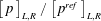 $\left[\,p\,\right]_{L,R}/\left[\,p^{ref}\,\right]_{L,R}$
, computed with (4.1) by Brennen (Reference Brennen1995) (variant
 $A$
, — - —) and by Rankine–Hugoniot analysis (equation (4.4a,b
), variant
 $B$
, ——; equation (4.4b
), variant
 $C$
, – –).
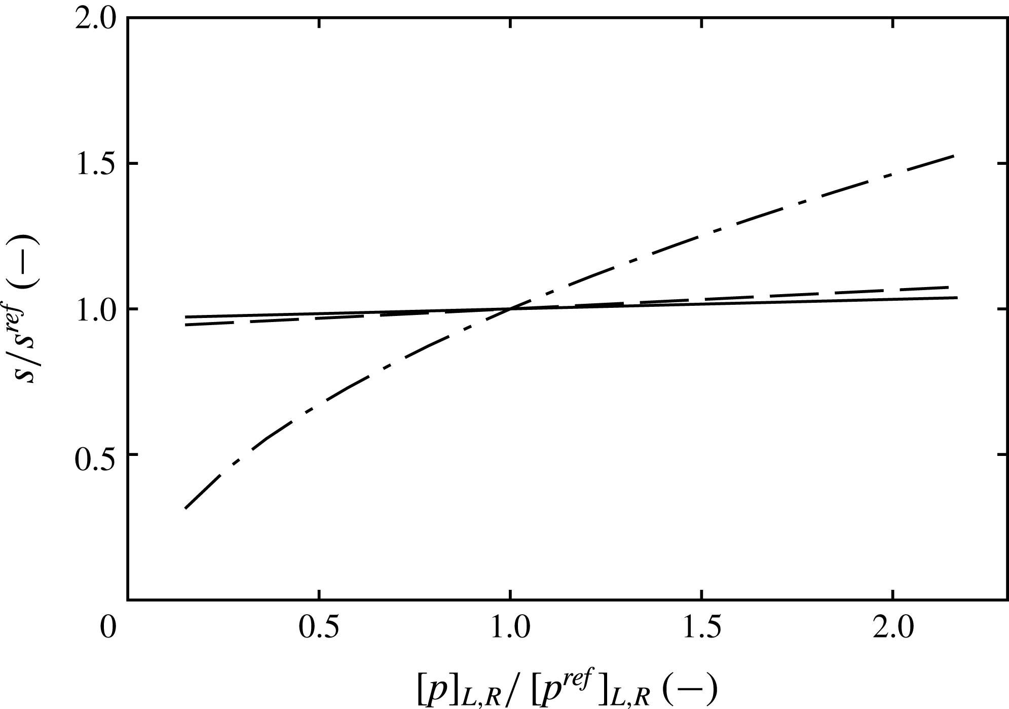
The sensitivity of the computed velocities is summarised in figure 21, plotting the normalised velocities
 $s/s^{ref}$
versus
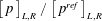 $\left[\,p\,\right]_{L,R}/\left[\,p^{ref}\,\right]_{L,R}$
. The Rankine–Hugoniot analysis is insensitive to the pressure rise: a
 $\pm 10\,\%$
difference in
 $\left[\,p\,\right]_{L,R}$
leads to a change in the predicted propagation velocity of at most
 $\pm 0.7\,\%$
. In contrast, Brennen’s formula shows a considerably larger sensitivity of
 $\pm 8\,\%$
for the same variation in the pressure rise.
While (4.1) gives reasonable results for the values from the mid-span slice, a considerably lower shock speed of
 $\langle s\rangle _{z}^{A}=-3.04~\text{m}~\text{s}^{-1}$
is obtained by using the spanwise-averaged values. The reason is the observed strong sensitivity of Brennen’s formula to the pressure difference in combination with the fact that the pressure difference in the spanwise average is lower than for the discrete slice,
 $\left[\,\langle p\rangle _{z}\,\right]_{L,R}<\left[\,p\,\right]_{L,R}$
. Hence, the shock speed computed with (4.1) is considerably affected by the degree of variation in the spanwise direction. This is not the case for the Rankine–Hugoniot analysis, which gives comparable values for the spanwise averages and the discrete slices, and is less sensitive to the pressure rise.
With the simulation, flow field data can be extracted at any position in the computational domain, including taking spanwise-averaged data. Thus, a clear distinction between the two approaches is possible. For the experimental data, on the other hand, some care has to be taken. Void fraction measurements as obtained by the x-ray densitometry are only available as spanwise averages, while the pressure is measured by pressure probes at discrete positions in the field.
5 Conclusions
The formation of cloud cavitation, classically associated with re-entrant jets, can also be caused by the occurrence of condensation shocks. This has been predicted previously by numerical simulations (Schmidt et al. Reference Schmidt, Thalhamer and Schnerr2009; Eskilsson & Bensow Reference Eskilsson and Bensow2012). However, a direct observation by experimental studies (see Ganesh et al. Reference Ganesh, Mäkiharju and Ceccio2016) has become available only recently. These authors suggest that condensation shocks represent an additional instability mechanism of partial cavitation. The motivation for our research is to obtain further insight into the physics of condensation shock phenomena, with the help of numerical simulations.
Based on the experiments by Ganesh et al. (Reference Ganesh, Mäkiharju and Ceccio2016), a validation of the numerical results is carried out. We focus on an operating point where periodic cloud shedding and the formation of upstream-travelling condensation shocks occur. The computational set-up reproduces the nominal definition of the experiments, including all variations of cross-section within the up- and downstream duct. We avoid the assumption of spanwise periodicity within the test section. The physical model is based on the homogeneous mixture approach, equilibrium thermodynamics and a barotropic equation of state. By neglecting the physical viscosity, we concentrate on the inertia-dominated flow physics. Compressibility of the two-phase flow is retained in the numerical method. Utilising explicit integration in time, all relevant time scales of cavitating flow are resolved. The method captures cavitation-induced shock-wave dynamics and its interaction with phase transition.
Our computations are in good agreement with most of the experimental results. Typical flow patterns occurring during shedding are well reproduced. In particular, sheet and cloud cavitation, inhomogeneous flow topology in the spanwise direction, cavitating horseshoe and hairpin vortices as well as crescent-shaped regions are found in the simulations. Furthermore, the growth and collapse speeds of the partial cavity are well matched. The comparison of the shedding Strouhal number and the evolution of the shedding process indicates that the global system dynamics are in good agreement.
Excellent match is observed for the spanwise-averaged vapour volume fraction within cavity sheets, reaching values of
 ${>}80\,\%$
. In individual slices, void fractions may locally exceed
 ${>}90\,\%$
, suggesting that the sheets consist of large contiguous regions of vapour instead of individual bubbles. Within the downstream-propagating clouds, however, the predicted void fraction is larger compared with the measurements. This is attributed to the spatial resolution being insufficient to reproduce the full range of scales for cloud cavitation. Slight deviations are found in the overall regularity of the shedding cycles. It is suggested that stabilising mechanisms, such as viscous layers and free gas content, may lead to a reduction of scatter for individual shedding cycles. The observed intermittency of irregular growth phases and, less frequently, re-entrant jets is also noted experimentally.
We conclude that the investigated configuration is entirely dominated by inertial effects, phase transfer and wave dynamics. This conclusion is substantiated by an analytical model for the total pressure loss in the test section, relying on the assumption of steady inviscid flow. It is shown that most of the total pressure loss is not related to viscous effects. Instead, it results from the pressure imbalance caused by the presence of cavitation in the tunnel. Dominating all other loss mechanisms including viscous losses, it justifies the use of an inviscid flow model.
Contrasting results from the simplified barotropic and non-barotropic thermodynamic models shows that the temperature dependence of the fluid properties are negligible. We further analyse the mechanisms of vortex stretching, compressible dilatation and baroclinic torque in our computations using the full thermodynamic model. We find that the baroclinic vorticity production is approximately one order of magnitude smaller than the combined effects of vortex stretching and compressible dilatation. The investigation substantiates that the baroclinic torque is only of subordinate importance. Once vorticity is introduced initially into the flow, vortex stretching due to shear, as well as dilatation due to flow compressibility, dominates the subsequent evolution of vorticity. A significant amount of vorticity is produced by the condensation shock front. As it is highly corrugated and of varying strength, this discontinuity causes the generation of vorticity in both the spanwise and streamwise directions. The upstream-propagating front is subject to Rayleigh–Taylor instabilities, while the postshock liquid undergoes Kelvin–Helmholtz instabilities.
In agreement with the experiments, the simulations identify a recurring condensation shock phenomenon as the main mechanism for cloud shedding. The predictions closely correspond to the experimentally observed behaviour. The fronts span almost the entire height of the cavity, and only a weak pressure increase across the front is detected. The computed propagation velocity closely agrees with the experimentally determined value. It is further found that the direction of flow is reversed behind the front, similarly to re-entrant jets. In contrast to the latter, however, upstream-directed flow is induced across most of the cavity height. It thus is not possible to stop the front by a small obstacle and suppress the associated cloud shedding, as already found experimentally by Ganesh et al. (Reference Ganesh, Mäkiharju and Ceccio2015). The aforementioned inviscid Rayleigh–Taylor and Kelvin–Helmholtz instabilities contribute to a thickening of the front in the spanwise average, while appearing sharp in individual slices.
Our simulations show that condensation shocks are, just like re-entrant jets, inertia-dominated features of partial cavities. It is demonstrated that the pre- and postshock flow states fulfil Rankine–Hugoniot jump conditions. The front thus represents a compressible shock wave, and analytical relations can be used to predict the shock strength and propagation velocity. We further contrast the Rankine–Hugoniot relations with the formula by Brennen (Reference Brennen1995) for computation of the propagation speed, including a sensitivity study regarding the pressure rise across the front. It is shown that Brennen’s formula is considerably more affected by this pressure difference, requiring an accurate determination of the latter for a proper prediction of the front velocity.
We find that condensation fronts can be triggered by shocks emanating from a downstream collapsing cloud. However, they are also observed under the absence of such events. This implies that the adverse pressure gradient is sufficient to induce a shock front. In addition to re-entrant jets, condensation shock phenomena thus feed an intrinsic instability mechanism of partial cavities.
Acknowledgements
Support for this research was provided by the US Office of Naval Research (ONR) and ONR Global through the NICOP entitled Numerical Investigation of Ship-Propeller Cavitation with Full Description of Shock-Wave Dynamics (Contract No. N62909-12-1-7034). We greatly acknowledge Dr K.-H. Kim (ONR HQs) and Dr W.-M. Lin (ONR Global) for their support and guidance throughout this project. We are especially grateful to Dr H. Ganesh and Professor S. Ceccio for providing detailed experimental data and the fruitful discussions on the subject. The authors further acknowledge the Gauss Centre for Supercomputing e.V. (GCS; www.gauss-centre.eu) for granting computational resources on the GCS Supercomputer ‘SuperMUC’ at the Leibniz Supercomputing Centre (LRZ; www.lrz.de).
Appendix A. Speed of sound in cavitating flow
In order to obtain a barotropic equation of state
 $\hat{p}(\hat{\unicode[STIX]{x1D70C}})$
for the mixture region, an estimate for the speed of sound
 $c$
in a two-phase flow is needed. Assuming a homogeneous mixture, i.e. neglecting bubble dynamics and surface tension, Brennen (Reference Brennen1995) and Franc & Michel (Reference Franc and Michel2005) derived analytical relations for
 $c$
. These authors discussed two limiting cases, which denote upper and lower estimates for the mixture speed of sound.
For the case of infinitely slow phase change, the speed of sound can be modelled as the frozen speed of sound
 $c_{fr}$
,
 $$\begin{eqnarray}\displaystyle & \displaystyle \frac{1}{\unicode[STIX]{x1D70C}c_{fr}^{2}}=\frac{\unicode[STIX]{x1D6FC}}{\unicode[STIX]{x1D70C}_{v,sat}c_{v}^{2}}+\frac{1-\unicode[STIX]{x1D6FC}}{\unicode[STIX]{x1D70C}_{l,sat}c_{l}^{2}}, & \displaystyle\end{eqnarray}$$
where the speeds of sound in the pure liquid and pure vapour are
 $c_{l}$
and
 $c_{v}$
respectively.
When both phases are in thermodynamic equilibrium, i.e. in the case of infinitely fast heat exchange between phases and thus phase change, the latent heat of vaporisation has to be taken into account on the right-hand side of (A 1). The speed of sound is then modelled with the equilibrium speed of sound
 $c_{eq}$
,
 $$\begin{eqnarray}\displaystyle & \displaystyle \frac{1}{\unicode[STIX]{x1D70C}c_{eq}^{2}}=\frac{\unicode[STIX]{x1D6FC}}{\unicode[STIX]{x1D70C}_{v,sat}c_{v}^{2}}+\frac{1-\unicode[STIX]{x1D6FC}}{\unicode[STIX]{x1D70C}_{l,sat}c_{l}^{2}}+\frac{(1-\unicode[STIX]{x1D6FC})\unicode[STIX]{x1D70C}_{l,sat}c_{p,l}T}{(\unicode[STIX]{x1D70C}_{v,sat}l_{v,ref})^{2}}. & \displaystyle\end{eqnarray}$$
In the barotropic model, the specific heat capacity of the liquid,
 $c_{p,l}=$
 $4184.4~\text{J}~\text{kg}^{-1}~\text{K}^{-1}$
, and the latent heat of evaporation,
 $l_{v,ref}=2453.5\times 10^{3}~\text{J}~\text{kg}^{-1}$
, are assumed to be constant at the constant reference temperature
 $T_{ref}$
.
A comparison of these two analytical relations for
 $c$
as a function of the void fraction
 $\unicode[STIX]{x1D6FC}$
is given in figure 22. As shown in figure 22(a), both yield a strong decrease for the speed of sound in the mixture region, being at least two orders of magnitude lower than the speed of the sound in either the pure liquid,
 $c_{l}\approx 1482~\text{m}~\text{s}^{-1}$
, or the pure vapour,
 $c_{v}\approx 423~\text{m}~\text{s}^{-1}$
. The frozen speed of sound exhibits a global minimum of
 $\min (c_{fr})=3.51~\text{m}~\text{s}^{-1}$
at
 $\unicode[STIX]{x1D6FC}=0.5$
, while the equilibrium speed of sound is minimal for
 $\unicode[STIX]{x1D6FC}\rightarrow 0^{+}$
with
 $\min (c_{eq})=0.038~\text{m}~\text{s}^{-1}$
. Figure 22(b) illustrates the ratio
 $c_{fr}/c_{eq}$
. In the region of relevant void fractions, the two approaches differ by a factor ranging between 10 (
 $\unicode[STIX]{x1D6FC}=0.95$
) and 140 (
 $\unicode[STIX]{x1D6FC}=0.1$
).


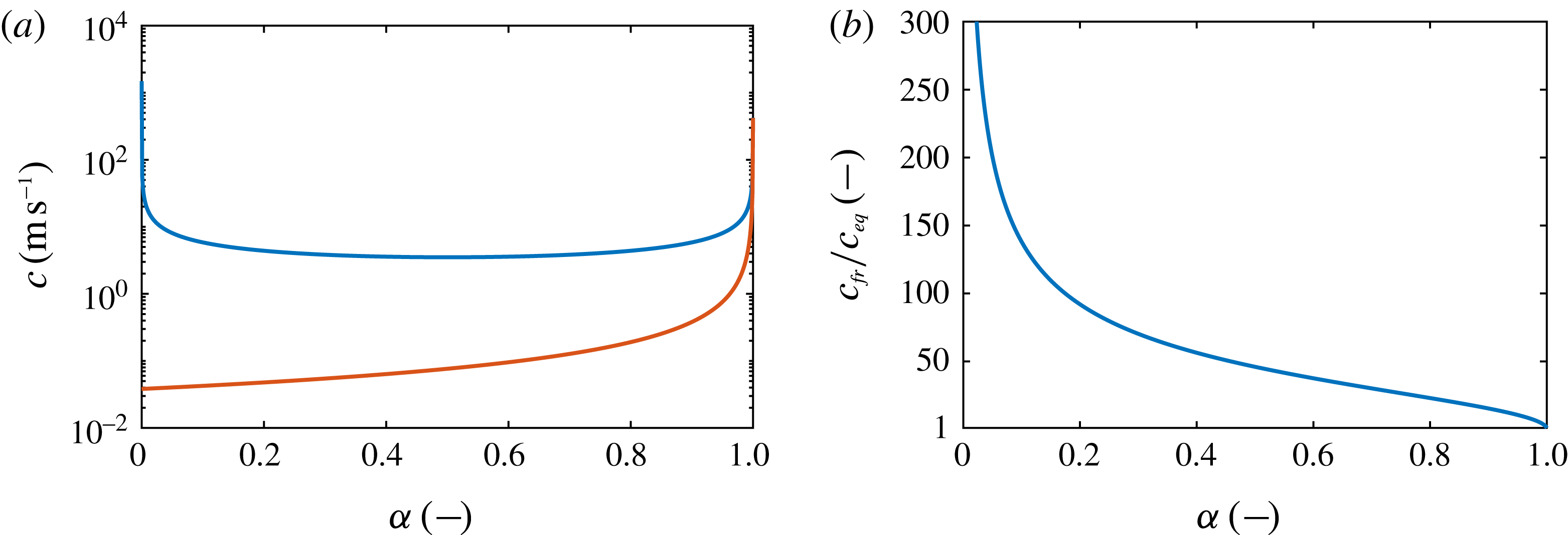
Brennen (Reference Brennen1995) discussed that the behaviour of a real two-phase medium lies in between these two extremes. The actual physical value is mainly controlled by the ‘degree of thermal exchange between the phases’. While perfect thermal exchange is assumed for the equilibrium speed of sound, the frozen speed of sound derives from the assumption of no exchange between the phases. However, the actual value of
 $c$
is difficult to measure experimentally, and may be problem-dependent. In either case, the mixture speed of sound may easily attain values smaller than the convective flow velocity in a technical system. Resulting in locally supersonic flow, this supports the occurrence of compressible shock-wave phenomena in the two-phase flow.
In the barotropic model, the assumed mixture speed of sound directly influences the level of vaporisation. With the definition of the speed of sound
 $$\begin{eqnarray}\displaystyle & \displaystyle c^{2}=\left.\frac{\unicode[STIX]{x2202}p}{\unicode[STIX]{x2202}\unicode[STIX]{x1D70C}}\right|_{s} & \displaystyle\end{eqnarray}$$
and the mixture density
 $\unicode[STIX]{x1D70C}=\unicode[STIX]{x1D6FC}\unicode[STIX]{x1D70C}_{v,sat}+(1-\unicode[STIX]{x1D6FC})\unicode[STIX]{x1D70C}_{l,sat}$
, it immediately follows that
 $$\begin{eqnarray}\displaystyle & \displaystyle \unicode[STIX]{x2202}\unicode[STIX]{x1D6FC}=\frac{1}{c^{2}}\frac{\unicode[STIX]{x2202}p}{\unicode[STIX]{x1D70C}_{v}-\unicode[STIX]{x1D70C}_{l}}. & \displaystyle\end{eqnarray}$$
Any change in pressure thus leads to a change in the vapour volume fraction, which is proportional to the square of the inverse speed of sound. Recognising that
 $c_{fr}\rightarrow c_{l}$
for
 $\unicode[STIX]{x1D6FC}\rightarrow 0$
, the integration of (A 4) with the frozen speed of sound shows that essentially no vapour is produced. This is in agreement with the assumption of the frozen model, but can thus not be used in the simulations. Still relying on the frozen speed of sound, an upper estimate for the produced vapour is to assume a constant mixture speed of sound equal to the global minimum,
 $\min (c_{fr})=3.51~\text{m}~\text{s}^{-1}$
. The maximum pressure difference is obtained when hypothetically expanding the mixture from the vapour pressure
 $p_{sat}$
to the triple line
 $p_{triple}$
. Even under these assumptions, the maximum attainable vapour volume fraction is
 $14\,\%$
. In contrast, as shown by Ganesh et al. (Reference Ganesh, Mäkiharju and Ceccio2016), the maximum void fraction observed for the current problem exceeds
 $80\,\%$
.
From these considerations, it is concluded that the frozen speed of sound is not suitable for the employed barotropic model and the present configuration. On the other hand, in order to accurately model the influence of thermal exchange between phases, additional assumptions are necessary, e.g. on interface areas, bubble size distributions and temperature gradients. None of these relevant parameters are available, either from experiments or from scale-resolved simulations. Without involving further assumptions, we chose the equilibrium speed of sound for the barotropic equation of state.
Appendix B. Assessment of the thermodynamic model
In the following, the influence of the thermodynamic modelling on the global system behaviour is reviewed. The importance of temperature dependence of the fluid properties in the modelling, the role of the barotropic assumption and the need to evolve the energy equation are assessed.
B.1 Isolated condensation shock
The dynamics of the sheet-to-cloud cavitation for the problem at hand is dominated by the repeated occurrence of condensation shocks. Capture of the associated entropy increases requires one to solve for the energy equation. In contrast, not accounting for these influences may cause an alteration of the shock speed or strength, and, hence, may affect the shedding dynamics.
The influence of the thermodynamic model is first studied with regard to isolated propagating condensation shocks, represented by simplified cases of one-dimensional Riemann problems. The computational domain utilised for this study is shown in figure 23. A total of 1000 homogeneously spaced cells are used for discretising the region of interest,
 $|x|\leqslant 1~\text{m}$
. To decouple the boundaries from the interior, the flow is extrapolated at the boundaries, located at
 $|x|=10~\text{m}$
, and a very coarse mesh is used for the region
 $1~\text{m}\leqslant |x|\leqslant 10~\text{m}$
. Here,
 $n=80$
cells are used, which are spaced according to an exponential bunching law,
 $Sp_{i}=Sp_{1}\cdot i\cdot \exp (R(i-1))$
. Here,
 $Sp_{i}$
denotes the distance from the starting point to node
 $i$
,
 $1\leqslant i\leqslant n$
, and the ratio
 $R=-\log \lfloor (n-1)Sp_{1}\rfloor /(n-2)$
.
The computational domain employed for the one-dimensional Riemann problem study, with
 $n$
denoting the number of cells along the respective edge.

For initialisation, ‘left’ and ‘right’ states are extracted from representative pre- and postshock states at discrete locations in the full three-dimensional simulations presented below. In general, the flow direction is reversed across the shock, while only a weak jump in pressure occurs. The vapour volume fraction upstream of the shock attains values between 80 % and 97 %, while complete condensation occurs after the front has passed.
Initial states at
 $t=0$
for the representatively considered one-dimensional Riemann problem, extracted from three-dimensional simulation. The initial temperature applies only for the full thermodynamic simulation and is computed from the internal energy.

Results of this Riemann study are exemplified here by one set of ‘left’ and ‘right’ states, given in table 8. For the full thermodynamic simulation, additional specification of the internal energy is necessary. It is chosen such that the ‘left’ and ‘right’ pressures and densities match for the two models. The chosen initialisation yields a left-running condensation front. Figure 24 shows a comparison of the results obtained with the barotropic and full thermodynamic models after integrating until
 $t=0.14~\text{s}$
. Results are provided in terms of the density
 $\unicode[STIX]{x1D70C}$
, velocity
 $u$
and void fraction
 $\unicode[STIX]{x1D6FC}$
. For the full thermodynamic simulation, the temperature difference
 $T-T_{0}$
is also provided, where
 $T_{0}$
is the initial temperature of the ‘left’ state.
One-dimensional Riemann problem, initialised with the states given in table 8, showing (a) density
 $\unicode[STIX]{x1D70C}$
, (b) velocity
 $u$
, (c) void fraction
 $\unicode[STIX]{x1D6FC}$
and (d) temperature difference
 $T-T_{0}$
. Comparison between the initial state at
 $t=0~\text{s}$
(— —) and results at
 $t=0.14~\text{s}$
obtained with the barotropic thermodynamic model (——, blue) and the full thermodynamic model (– – –, red).

For
 $\unicode[STIX]{x1D70C}$
,
 $u$
and
 $\unicode[STIX]{x1D6FC}$
, the two models yield comparable results, and the left-running shock is located at the same position. The propagation velocity of the front can thus be evaluated equally as
 $u_{shock}=-5.18~\text{m}~\text{s}^{-1}$
. The obtained value for
 $u_{shock}$
is in good agreement with the result of the full three-dimensional computations. Temperature variations predicted with the full thermodynamic model are small. The temperature increase across the shock amounts to
 $\max (T-T_{0})=0.077~\text{K}$
as the observed condensation shock is very weak. The associated entropy production can be neglected.
The presented analysis is repeated with various pre- and postshock states, extracted from the full three-dimensional simulations. From these investigations, it is deduced that the thermodynamic model has no measurable influence regarding the computed velocity and strength for the considered low-speed condensation fronts occurring in the present case. This provides an indication that the barotropic model is able to correctly predict the shock-dominated cavitating flow dynamics for the problem at hand.
B.2 Full thermodynamic simulation
In order to assess the influence of the thermodynamic model on the flow dynamics, three-dimensional simulations are carried out using both thermodynamic approaches. Statistics on the
 $\mathit{lvl}_{2}$
grid are collected with a sampling interval of
 $0.39\times 10^{-6}~\text{s}$
. For the barotropic model, the sampling spans
 $1.66~\text{s}$
, while the statistics of the full thermodynamic model cover
 $1.54~\text{s}$
.
Only marginal differences are found between the two simulations; see figures 25(a,b) and 25(c,d) for a juxtaposition of the spanwise average of the temporal mean and RMS of the void fraction,
 $\langle \overline{\unicode[STIX]{x1D6FC}}\rangle _{z}$
and
 $\langle \overline{\unicode[STIX]{x1D6FC}^{\prime }\unicode[STIX]{x1D6FC}^{\prime }}\rangle _{z}^{1/2}$
respectively, obtained on the
 $\mathit{lvl}_{2}$
grid. Small deviations between the models are attributed primarily to the different sampling times in conjunction with the chaotic nature and the associated cycle-to-cycle variations of the shedding process.
Comparison of (a,b) the span- and time-averaged void fraction field
 $\langle \overline{\unicode[STIX]{x1D6FC}}\rangle _{z}$
and (c,d) the span- and time-averaged RMS of the void fraction field
 $\langle \overline{\unicode[STIX]{x1D6FC}^{\prime }\unicode[STIX]{x1D6FC}^{\prime }}\rangle _{z}^{1/2}$
. Juxtaposition of results obtained with the barotropic model (a,c) and the full thermodynamic model (b,d).

Furthermore, the models are analysed with regard to their spectral content. For this purpose, Welch’s method for estimating the spectral density is applied to the operating-point-defining quantities
 $u_{1}$
,
 $p_{1}$
,
 $p_{2}$
at locations
 $1$
and
 $2$
, as well as the pressure
 $p_{P_{D}}$
and local void fraction
 $\unicode[STIX]{x1D6FC}_{P_{D}}$
at probing position
 $P_{D}$
. The signals are sampled with a time resolution of
 $0.4\times 10^{-6}~\text{s}$
and then linearly interpolated on a constant time step of
 $1\times 10^{-6}~\text{s}$
. The spectra are estimated using Hanning window segments with equal window length in a time domain of
 $0.2~\text{s}$
and
 $50\,\%$
overlap between subsequent segments. The resulting spectra are given in figure 26. Signals recorded in the vicinity of the wedge, namely
 $p_{1}$
,
 $p_{P_{D}}$
and
 $\unicode[STIX]{x1D6FC}_{P_{D}}$
, exhibit a dominant low frequency
 $f_{1}$
, which is the shedding frequency of the sheet cavity. For both models,
 $f_{1}^{\mathit{lvl}_{2},baro}\approx 19.1~\text{Hz}\approx f_{1}^{\mathit{lvl}_{2},full}$
. Together with an almost identical prediction of the attached sheet length, the associated shedding Strouhal numbers obtained with the two models hence are also comparable. Deviations in the spectra are attributed to the different numbers of shedding cycles covered with the statistics in conjunction with the cycle-to-cycle variations.
Frequency spectra of time signals of (a) upstream velocity
 $u_{1}$
, (b) upstream pressure
 $p_{1}$
, (c) downstream pressure
 $p_{2}$
, (d) pressure at
 $P_{D}$
and (e) local void fraction at
 $P_{D}$
. Comparison of numerical prediction on the grid
 $\mathit{lvl}_{2}$
using the barotropic (blue) and the full thermodynamic model (red).

The span- and time-averaged temperature field
 $\langle \overline{T}\rangle _{z}$
and the associated RMS
 $\langle \overline{T^{\prime }T^{\prime }}\rangle _{z}^{1/2}$
predicted with the full thermodynamic model are given in figure 27(a,b). The visualisations show that the mean temperature within the cavity drops by less than
 $0.3~\text{K}$
and that the RMS of the temperature attains values of at most
 $0.5~\text{K}$
. In these ranges, the associated variation of fluid properties hence is negligible and the assumption of constant properties in the barotropic model is justified.
Temperature variations predicted by the full thermodynamic model. Juxtaposition of (a) the span- and time-averaged temperature
 $\langle \overline{T}\rangle _{z}$
(with colour gradation changes at equally spaced intervals of 0.02 K) and (b) the span- and time-averaged RMS of the temperature
 $\langle \overline{T^{\prime }T^{\prime }}\rangle _{z}^{1/2}$
.

Moreover, the budgets of the VTE, describing the evolution of the vorticity
 $\unicode[STIX]{x1D74E}$
along a particle path, are assessed. The VTE is given as follows:
 $$\begin{eqnarray}\displaystyle & \displaystyle \frac{\text{D}}{\text{D}t}\unicode[STIX]{x1D74E}=\underbrace{\left(\unicode[STIX]{x1D74E}\boldsymbol{\cdot }\unicode[STIX]{x1D735}\right)\boldsymbol{u}}_{=\unicode[STIX]{x1D74A}_{1}}-\underbrace{\unicode[STIX]{x1D74E}\left(\unicode[STIX]{x1D735}\boldsymbol{\cdot }\boldsymbol{u}\right)}_{=\unicode[STIX]{x1D74A}_{2}}+\underbrace{\frac{1}{\unicode[STIX]{x1D70C}^{2}}\hspace{2.22198pt}\unicode[STIX]{x1D735}\unicode[STIX]{x1D70C}\times \unicode[STIX]{x1D735}p}_{=\unicode[STIX]{x1D74A}_{3}}. & \displaystyle\end{eqnarray}$$
The material derivative of the vorticity is denoted by
 $\text{D}/\text{D}t\,\unicode[STIX]{x1D74E}$
, and the three terms
 $\unicode[STIX]{x1D74A}_{1}$
,
 $\unicode[STIX]{x1D74A}_{2}$
,
 $\unicode[STIX]{x1D74A}_{3}$
can be identified as the vortex stretching due to velocity gradients, flow compressibility (compressible dilatation) and baroclinic torque respectively. In order to assess the relative importance of these budgets in the full thermodynamic simulation, we further define the following integrals:
 $$\begin{eqnarray}\displaystyle & \displaystyle \unicode[STIX]{x1D6F6}_{1}=\frac{1}{V}\int _{\unicode[STIX]{x1D6FA}}\langle \overline{\left|\unicode[STIX]{x1D74A}_{1}\right|}\rangle _{z}\,\hspace{2.22198pt}\text{d}V,\quad \unicode[STIX]{x1D6F6}_{2}=\frac{1}{V}\int _{\unicode[STIX]{x1D6FA}}\langle \overline{\left|\unicode[STIX]{x1D74A}_{2}\right|}\rangle _{z}\hspace{2.22198pt}\hspace{2.22198pt}\text{d}V,\quad \unicode[STIX]{x1D6F6}_{3}=\frac{1}{V}\int _{\unicode[STIX]{x1D6FA}}\langle \overline{\left|\unicode[STIX]{x1D74A}_{3}\right|}\rangle _{z}\hspace{2.22198pt}\hspace{2.22198pt}\text{d}V. & \displaystyle \nonumber\\ \displaystyle & & \displaystyle\end{eqnarray}$$
Figure 28(a–c) shows the time- and spanwise-averaged budgets of
 $\langle \overline{|\unicode[STIX]{x1D74A}_{1}|}\rangle _{z}$
,
 $\langle \overline{|\unicode[STIX]{x1D74A}_{2}|}\rangle _{z}$
and
 $\langle \overline{|\unicode[STIX]{x1D74A}_{3}|}\rangle _{z}$
, while figure 28(d) compares the integral magnitudes
 $\unicode[STIX]{x1D6F6}_{1},\unicode[STIX]{x1D6F6}_{2},\unicode[STIX]{x1D6F6}_{3}$
. The visualisation shows that in the full thermodynamic computation, the baroclinic torque is predominately active at the liquid–vapour interface, with the strongest contribution in close vicinity to the wedge apex. In contrast, contributions due to vortex stretching and compressible dilatation can be found throughout the cavitating region, exceeding the baroclinic torque by at least a factor of 2 in close vicinity to the liquid–vapour interface, or well above within the cavitating region. The integral budgets in figure 28(d) further show that the baroclinic torque is approximately one order of magnitude smaller than the combined effects of vortex stretching and compressible dilatation.
Assessment of the VTE budgets. Time- and spanwise-averaged field of (a) vortex stretching
 $\langle \overline{|\unicode[STIX]{x1D74A}_{1}|}\rangle _{z}$
, (b) compressible dilatation
 $\langle \overline{|\unicode[STIX]{x1D74A}_{2}|}\rangle _{z}$
and (c) baroclinic torque
 $\langle \overline{|\unicode[STIX]{x1D74A}_{3}|}\rangle _{z}$
. (d) Juxtaposition of integral budgets
 $\unicode[STIX]{x1D6F6}_{1}$
,
 $\unicode[STIX]{x1D6F6}_{2}$
and
 $\unicode[STIX]{x1D6F6}_{3}$
.

The physical process of vorticity production through baroclinic torque
 $\unicode[STIX]{x1D74A}_{3}$
cannot be reproduced when employing a barotropic model, where the gradients of the density
 $\unicode[STIX]{x1D735}\unicode[STIX]{x1D70C}$
and the pressure
 $\unicode[STIX]{x1D735}p$
are parallel. A significant amount of vorticity is, however, produced by the condensation shock front. As it is highly corrugated and of varying strength, this discontinuity causes the generation of vorticity in both the spanwise and streamwise directions. The upstream-propagating front is further subject to Rayleigh–Taylor instabilities, while the postshock liquid undergoes Kelvin–Helmholtz instabilities. Additionally, a small amount of vorticity production is also associated with the numerical regularisation (
 $=$
artificial viscosity), which is inevitable for discontinuity-capturing.
From the analysis of the VTE budgets, we conclude that, once vorticity is introduced initially into the flow, vortex stretching due to shear as well as dilatation due to flow compressibility entirely dominate the subsequent evolution of vorticity.
In summary, the influence of the thermodynamic model is insignificant for the considered configuration.
Appendix C. Pressure drop
In order to assess the influences contributing to a larger pressure loss across the test section in the simulation compared with the experiment, an analytical model for
 $\unicode[STIX]{x0394}p$
between stations 1 and 2 is derived in the following. Figure 29 provides a sketch of the considered simplified configuration. The flow in the test section is assumed to be inviscid, stationary and two-dimensional. Furthermore, the inflow and outflow velocities are taken as equal,
 $u_{1}\approx u_{2}$
. This can be readily derived from continuity through the test section, and assuming complete recondensation before the flow exits the test section at station 2. Finally, it is assumed that the quantities
 $u_{1}$
,
 $u_{2}$
,
 $p_{1}$
and
 $p_{2}$
act across the entire inflow and outflow plane of the test section, which is reasonably accurate for the following derivation. Under these assumptions, the pressure drop is solely caused by pressure contributions along walls, with a non-vanishing normal vector in the direction of the flow,
 $$\begin{eqnarray}\displaystyle & \displaystyle \unicode[STIX]{x0394}p=\frac{1}{A_{ch}}\int _{A}p([1,0,0]^{\text{T}}\cdot \boldsymbol{n})\hspace{2.22198pt}\text{d}S. & \displaystyle\end{eqnarray}$$
Here,
 $A_{ch}$
denotes the channel cross-section, while
 $\boldsymbol{n}$
is the inward-pointing unit normal vector on the integration surfaces. Only the upstream and downstream shoulders of the wedge contribute to the pressure drop.
By assuming a pressure distribution along the wedge surface, (C 1) can be solved analytically. The total pressure of the flow entering the test section is given by the upstream station 1 as
 $p_{t}=p_{1}+\unicode[STIX]{x1D70C}_{1}u_{1}^{2}/2$
. The pressure at the edge between the bottom wall and the upstream shoulder of the wedge is assumed to be
 $\unicode[STIX]{x1D701}_{1}p_{t}$
. An inviscid flow model requires a stagnation point at this location, i.e.
 $\unicode[STIX]{x1D701}_{1}=1$
. Under the presence of a viscous boundary layer, the total pressure is only partly recovered, and thus
 $0<\unicode[STIX]{x1D701}_{1}<1$
for viscous flow. Originating at the apex and extending over a fraction
 $\unicode[STIX]{x1D709}$
of the back side of the wedge with length
 $L_{w}$
, a cavity is present in the temporal mean. Accounting for the fact that, intermittently, both wetted and cavitating flow exist, the pressure in this region can be modelled as constant and equal to a multiple of the vapour pressure, i.e.
 $\unicode[STIX]{x1D701}_{2}p_{sat}$
, with
 $\unicode[STIX]{x1D701}_{2}\geqslant 1$
. For the upstream shoulder, a linear decrease from
 $\unicode[STIX]{x1D701}_{1}p_{t}$
to
 $\unicode[STIX]{x1D701}_{2}p_{sat}$
at the apex is assumed. The pressure recovery downstream of the cavity is also assumed to be linear, from
 $\unicode[STIX]{x1D701}_{2}p_{sat}$
to
 $\unicode[STIX]{x1D701}_{3}p_{t}$
, with
 $0<\unicode[STIX]{x1D701}_{3}<1$
. It should be noted that even for inviscid flow, no stagnation point can be assumed, as the region downstream of the cavity is largely affected by the passage of clouds shedding from the sheet cavity.
Sketch of the simplified test-section geometry utilised for the analytical pressure drop model, including an indication of the parameters
 $\unicode[STIX]{x1D701}_{1}$
,
 $\unicode[STIX]{x1D701}_{2}$
,
 $\unicode[STIX]{x1D701}_{3}$
and
 $\unicode[STIX]{x1D709}$
.

Integration of (C 1) with the assumed analytical pressure profile yields
 $$\begin{eqnarray}\displaystyle & \displaystyle \unicode[STIX]{x0394}p={\textstyle \frac{1}{6}}[p_{t}(\unicode[STIX]{x1D701}_{1}-(1-\unicode[STIX]{x1D709})\unicode[STIX]{x1D701}_{3})-\unicode[STIX]{x1D701}_{2}\unicode[STIX]{x1D709}p_{sat}]. & \displaystyle\end{eqnarray}$$
Under inviscid assumptions, i.e. with
 $\unicode[STIX]{x1D701}_{1}=1$
, and, for simplicity, assuming a stationary cavity that covers the entire back side of the wedge, i.e.
 $\unicode[STIX]{x1D701}_{2}=1,\unicode[STIX]{x1D709}=1$
, (C 2) reduces to
 $$\begin{eqnarray}\displaystyle & \displaystyle \unicode[STIX]{x0394}p={\textstyle \frac{1}{6}}[p_{t}-p_{sat}]. & \displaystyle\end{eqnarray}$$
This predicts a pressure loss of
 ${\approx}15~\text{kPa}$
, which clearly exceeds the experimentally observed value of
 $8.2~\text{kPa}$
. These considerations show that the present configuration generates a pressure loss even under inviscid assumptions. It thus is analogous to the generation of wave drag in inviscid supersonic flow. Here, it is caused solely by the presence of two-phase flow, which prevents a pressure recovery on the back side of the wedge.
In order to calibrate the parameters
 $\unicode[STIX]{x1D701}_{1}$
,
 $\unicode[STIX]{x1D701}_{2}$
,
 $\unicode[STIX]{x1D701}_{3}$
and
 $\unicode[STIX]{x1D709}$
, the assumed analytical pressure profile along the wedge surface is compared with the result obtained by the inviscid computations presented in the remainder of this paper. As shown in figure 30, the parameters
 $\unicode[STIX]{x1D701}_{1}=1$
,
 $\unicode[STIX]{x1D701}_{2}=4$
,
 $\unicode[STIX]{x1D701}_{3}=0.53$
and
 $\unicode[STIX]{x1D709}=0.6$
give good agreement with the numerical result. The computed analytical pressure drop (
 $12.3~\text{kPa}$
) compares well with a numeric integration of the profile shown in figure 30 (
 $12.7~\text{kPa}$
). Despite the simplifying assumptions of the presented analysis, the computed
 $\unicode[STIX]{x0394}p$
also compares reasonably well with the pressure loss given by the two point probes at locations 1 and 2, as stated in table 6 (
 $14~\text{kPa}$
).
The pressure along the bottom wall for the analytical pressure loss model. Comparison between the assumed analytical shape (——) with parameters
 $\unicode[STIX]{x1D701}_{1}=1$
,
 $\unicode[STIX]{x1D701}_{2}=4$
,
 $\unicode[STIX]{x1D701}_{3}=0.53$
,
 $\unicode[STIX]{x1D709}=0.6$
and the time-averaged pressure
 $\overline{p}_{bottom}$
as recorded from full three-dimensional simulation at mid-span along the bottom wall (– –).

Due to the boundary layer in the experiments, the total pressure is only partially recovered at the upstream edge between the wedge and the bottom wall, and thus
 $0<\unicode[STIX]{x1D701}_{1}<1$
. No experimental data are available that would allow for an estimation of
 $\unicode[STIX]{x1D701}_{1}$
. Thus, using the ANSYS CFX simulation package, incompressible single-phase simulations solving the Reynolds-averaged Navier–Stokes (RANS) equations are carried out. For this purpose, the same geometry, including all changes in the upstream and downstream ducts, as discussed in § 3 is utilised. Viscous walls are resolved with a wall-unit
 $y^{+}\lesssim 1$
in the upstream contraction leading to the test section and the vicinity of the wedge; turbulence modelling is carried out with the Baseline Explicit Algebraic Reynolds Stress model (BSL-EARSM). Inflow and outflow boundary conditions are chosen identical to the compressible simulation. These computations yield a value of
 $\unicode[STIX]{x1D701}_{1}/p_{t}\approx 0.82$
. Using this parameter in (C 2), in conjunction with the previously determined value of
 $\unicode[STIX]{x1D701}_{3}=0.53$
, and the experimental value for the cavity length of
 $\unicode[STIX]{x1D709}=0.53$
, this gives
 $\unicode[STIX]{x0394}p=8.1~\text{kPa}$
. This result is in good correspondence with the experimentally obtained pressure drop of
 $8.2~\text{kPa}$
. As viscous contributions are neglected in the model, this substantiates the fact that the losses due to the presence of two-phase flow dominate any other loss mechanisms, including losses due to viscosity.
Sensitivity study for the pressure drop estimated with (C 2), regarding (a) the cavity length and (b) the upstream pressure.

From this analytical model, two factors contributing to an overestimation of the pressure loss can be identified. First, in the case of a partial cavity, i.e. for
 $0<\unicode[STIX]{x1D709}<1$
, a larger cavity length, correlating with a larger cavity extent, causes an increase of
 $\unicode[STIX]{x0394}p$
. A second factor is the pressure
 $\unicode[STIX]{x1D701}_{1}p_{t}$
and the subsequent pressure distribution along the upstream shoulder of the wedge. The significance of these two aspects is assessed in figure 31. Keeping the parameters
 $\unicode[STIX]{x1D701}_{2}=4$
,
 $\unicode[STIX]{x1D701}_{3}=0.53$
fixed, the cavity length is studied in figure 31(a) via the parameter
 $\unicode[STIX]{x1D709}$
. The investigation is carried out for two upstream pressures
 $\unicode[STIX]{x1D701}_{1}=(0.82,1)$
, corresponding to the cases without and with recovery of the total pressure in the upstream corner of the wedge and the bottom wall respectively. A variation in the cavity length in the range
 $0.5\leqslant \unicode[STIX]{x1D709}\leqslant 1$
leads to a change in
 $\unicode[STIX]{x0394}p$
of at most
 $3.6~\text{kPa}$
. In figure 31(b), the parameter
 $\unicode[STIX]{x1D701}_{1}$
for the upstream pressure is varied, with the same parameters
 $\unicode[STIX]{x1D701}_{2}=4$
,
 $\unicode[STIX]{x1D701}_{3}=0.53$
and a fixed cavity length
 $\unicode[STIX]{x1D709}=0.6$
. With an influence of at most
 $8.3~\text{kPa}$
on
 $\unicode[STIX]{x0394}p$
when considering
 $0.5\leqslant \unicode[STIX]{x1D701}_{1}\leqslant 1$
, the pressure
 $\unicode[STIX]{x1D701}_{1}p_{t}$
also has a significant influence on the overall pressure drop.
The three-dimensional inviscid simulations give a cavity extent that is larger by approximately 12 %, compared with the experiments. As deduced from figure 31(a), this corresponds to an additional increase in the pressure drop according to this model of
 ${\approx}0.5~\text{kPa}$
. Furthermore, the total pressure is recovered at the upstream edge of the wedge in the simulations, which is not the case in the experiments. This latter aspect accounts for an additional pressure loss of approximately
 $2.8~\text{kPa}$
. Combined, the model estimates a deviation in the pressure loss of approximately
 $3.3~\text{kPa}$
, relying entirely on inviscid and steady-state assumptions. It can be assumed that under unsteady conditions, the pressure drop due to cavitation is larger, as, intermittently, cavitating regions including detaching cloudy structures may reach a much larger extent, causing a higher level of blockage in the channel. Regarding the simplifications in the derivations, most notably the assumption of two-dimensional stationary flow and neglect of viscous losses in the tunnel, this corresponds reasonably well with the observed difference of
 $6~\text{kPa}$
shown in table 6 between the predicted and experimental pressure losses.
It is shown by this model that the present configuration generates a pressure loss, even under inviscid assumptions. Furthermore, the pressure distribution on the upstream shoulder of the wedge has a larger influence than the overestimation of the cavity extent on the fact that the pressure loss in the computations is larger than that in the experiments. Due to the employed inviscid flow model, the total pressure is recovered at the upstream corner of the wedge and the bottom wall, which is not the case in the experiments. Besides its influence on the overall pressure loss, this has only limited influence on the system.
Appendix D. Upstream velocity
In order to assess the assumption of slip boundary conditions and their potential effect on the cavitating region, the upstream velocity profile at
 $x=-82~\text{mm}$
is analysed in the following. For this purpose, figure 32 shows the profile of the axial velocity component within the test section along the transverse direction at mid-span. The velocity is normalised by the upstream velocity at position
 $1$
as
 $\overline{u}/\overline{u}_{1}$
and the
 $y$
-coordinate by the channel height as
 $y/h_{ch}$
. The plot compares laser Doppler velocimetry (LDV) measurements by Ganesh et al. (Reference Ganesh, Mäkiharju and Ceccio2016), including an indication of the experimental uncertainty, with numerical predictions. Ganesh et al. (Reference Ganesh, Mäkiharju and Ceccio2016) conducted two sets of measurements, i.e. in the bulk and, with a higher spatial resolution, in the near-wall region. The two sets do not match exactly in the overlapping region
 $0.02\leqslant y/h_{ch}\leqslant 0.06$
, which is attributed to uncertainties in the measurements. The difference in the measured velocity, however, amounts to
 ${\lesssim}2\,\%$
, and can thus be regarded as negligible. The numerical data included in figure 32 encompass the inviscid computations discussed in the remainder of this paper, as well as the viscous but incompressible RANS computation conducted with ANSYS CFX, introduced in appendix C. The RANS represents steady single-phase computations, while the inviscid computations are transient and include phase change. Results of the latter thus are time-averaged. The presence of cavitation developing downstream of the wedge apex does not influence the investigated upstream velocity profile, as can be seen from the visualisation.
In the bulk, very good agreement with the references is found, with both numerical predictions being within the experimental error range. The viscous computations show a slightly higher velocity compared with the inviscid simulation. This is due to the displacement effect of the boundary layer while keeping the total mass flux through the velocity inlet boundary condition identical. With a deviation of
 ${\lesssim}1.5\,\%$
between the predictions, this effect is, however, negligible. The RANS computations exhibit good agreement with the experimental references also in the near-wall region. As expected from the employed slip boundary condition, the inviscid simulation shows no near-wall viscous layer. However, the differences are restricted to a region of less than 2 % of the channel height. Due to the subsequent acceleration of the flow on the convergent part of the wedge, the boundary layer is expected to be even thinner when reaching the sharp wedge apex.
Validation of the upstream velocity profile at
 $x=-82~\text{mm}$
. Comparison between experiments by Ganesh et al. (Reference Ganesh, Mäkiharju and Ceccio2016) (data from direct communication with H. Ganesh; measurements in the bulk, black, and near-wall profile, grey, including experimental uncertainty) and numerical predictions (compressible inviscid simulation, red solid line, and incompressible viscous simulation, red dashed line).

From this investigation, it is concluded that incoming near-wall viscous layers do not have a significant influence on the sheet cavity, and that the assumptions of inviscid flow and slip boundary conditions in the two-phase computations are acceptable.
The time evolution of the integral vapour content
 $V_{\unicode[STIX]{x1D6FC}}$
, predicted on different grid levels (
 $\mathit{lvl}_{0}$
, blue;
 $\mathit{lvl}_{1}$
, red;
 $\mathit{lvl}_{2}$
, yellow), including the respective time average (- - - -).

Appendix E. Grid convergence
Figure 33 shows the time evolution of the total amount of vapour volume in the complete domain,
 $V_{\unicode[STIX]{x1D6FC}}=\int _{\unicode[STIX]{x1D6FA}}\unicode[STIX]{x1D6FC}\,\text{d}V$
, together with an indication of the temporal mean,
 $\overline{V}_{\unicode[STIX]{x1D6FC}}$
, for all three grid levels
 $\mathit{lvl}_{0}$
,
 $\mathit{lvl}_{1}$
and
 $\mathit{lvl}_{2}$
. Compared with the two finer grid levels, the mean vapour volume predicted on
 $\mathit{lvl}_{0}$
is larger, and the dynamics differs noticeably. In contrast, grid levels
 $\mathit{lvl}_{1}$
and
 $\mathit{lvl}_{2}$
yield nearly the same mean integral vapour volume and also show comparable time evolutions. With
 $\langle \,\bullet \,\rangle _{z}$
denoting averaging in the spanwise direction, figure 34 shows the mean void fraction
 $\langle \overline{\unicode[STIX]{x1D6FC}}\rangle _{z}$
and the RMS of the vapour fluctuations
 $\langle \overline{\unicode[STIX]{x1D6FC}^{\prime }\unicode[STIX]{x1D6FC}^{\prime }}\rangle _{z}^{1/2}$
. In agreement with the above findings for
 $\overline{V}_{\unicode[STIX]{x1D6FC}}$
, the spatial extent of the mean vapour structures, figure 34(a–c), is largest on
 $\mathit{lvl}_{0}$
. Moreover, the RMS level of vapour fluctuations, figure 34(d–f), predicted on
 $\mathit{lvl}_{0}$
is higher compared with the two finer grid levels. On the other hand, the shape and extent of
 $\langle \overline{\unicode[STIX]{x1D6FC}}\rangle _{z}$
and
 $\langle \overline{\unicode[STIX]{x1D6FC}^{\prime }\unicode[STIX]{x1D6FC}^{\prime }}\rangle _{z}^{1/2}$
are almost identical for grids
 $\mathit{lvl}_{1}$
and
 $\mathit{lvl}_{2}$
.
Furthermore, the three grid levels are analysed with regard to the dominant frequencies present in the flow. For this purpose, Welch’s method for estimating the spectral density is applied to the operating-point-defining quantities
 $u_{1}$
,
 $p_{1}$
,
 $p_{2}$
at locations
 $1$
and
 $2$
, as well as the pressure
 $p_{P_{D}}$
and local void fraction
 $\unicode[STIX]{x1D6FC}_{P_{D}}$
at probing position
 $P_{D}$
. The signals are sampled with a time resolution as given in table 4 and then linearly interpolated on a constant time step of
 $2\times 10^{-6}~\text{s}$
(
 $\mathit{lvl}_{0}$
), and
 $1\times 10^{-6}~\text{s}$
(
 $\mathit{lvl}_{1}$
and
 $\mathit{lvl}_{2}$
). The spectra are estimated using Hanning window segments with equal window length in a time domain of
 $0.2~\text{s}$
and
 $50\,\%$
overlap between subsequent segments. The resulting spectra are given in figure 35.
Grid convergence of (a–c) time-averaged void fraction field
 $\langle \overline{\unicode[STIX]{x1D6FC}}\rangle _{z}$
and (d–f) time-averaged RMS of void fraction field
 $\langle \overline{\unicode[STIX]{x1D6FC}^{\prime }\unicode[STIX]{x1D6FC}^{\prime }}\rangle _{z}^{1/2}$
. Comparison between numerical prediction on (a,d)
 $\mathit{lvl}_{0}$
, (b,e)
 $\mathit{lvl}_{1}$
and
 $(c,\mathit{f}\,)$
 $\mathit{lvl}_{2}$
.

Frequency spectra of time signals of (a) upstream velocity
 $u_{1}$
, (b) upstream pressure
 $p_{1}$
, (c) downstream pressure
 $p_{2}$
, (d) pressure at
 $P_{D}$
and (e) local void fraction at
 $P_{D}$
. Comparison of numerical prediction on different grid levels (
 $\mathit{lvl}_{0}$
, blue;
 $\mathit{lvl}_{1}$
, red;
 $\mathit{lvl}_{2}$
, yellow).

Signals recorded in the vicinity of the wedge, namely
 $p_{1}$
,
 $p_{P_{D}}$
and
 $\unicode[STIX]{x1D6FC}_{P_{D}}$
, exhibit a dominant low frequency
 $f_{1}$
on all three grid levels. This frequency can be identified as the shedding frequency of the sheet cavity. For
 $\mathit{lvl}_{0}$
,
 $f_{1}^{\mathit{lvl}_{0}}\approx 11.4~\text{Hz}$
, which is lower than on the two finer grids. This in accordance with the larger extent of the sheet cavity on this grid level, as seen above. For
 $\mathit{lvl}_{1}$
and
 $\mathit{lvl}_{2}$
, the computed shedding frequencies are in excellent agreement, with
 $f_{1}^{\mathit{lvl}_{1}}\approx 19.1~\text{Hz}\approx f_{1}^{\mathit{lvl}_{2}}$
. The dominant frequencies for the signals of
 $u_{1}$
and
 $p_{2}$
also agree for
 $\mathit{lvl}_{1}$
and
 $\mathit{lvl}_{2}$
. In contrast, grid
 $\mathit{lvl}_{0}$
shows discrepancies both in the dominant frequencies as well as in the integral power of the spectrum, indicating that the cavity dynamics is not sufficiently resolved on this level.
Minor deviations in the spectral power can be observed also between
 $\mathit{lvl}_{1}$
and
 $\mathit{lvl}_{2}$
. This is associated with a higher level of fragmentation of vapour structures on finer grid levels when using a formally inviscid modelling approach. This fragmentation leads to a grid dependence of peak pressures and cavity collapse rates, which in turn affects the level of recorded pressure fluctuations and thus spectra; see the in-depth discussion by Mihatsch et al. (Reference Mihatsch, Schmidt and Adams2015). As seen from figure 35, this does not alter the predicted low-frequency shedding of the sheet cavity. This mechanism is governed by the intrinsic instability of the cavity and the occurrence of the condensation shock phenomenon, which is of primary interest for the current paper.
It should be noted that when utilising an inviscid approach, classical grid convergence cannot be expected, since no viscous limiting length scale exists. From this study, we conclude that
 $\mathit{lvl}_{2}$
is grid-converged with respect to the integral length scales of the flow and the global dynamics of the system.