1 Introduction
The conversion of large-scale available potential energy to mesoscale eddy energy by baroclinic instability is one of the most important energy pathways in the global ocean (Ferrari & Wunsch Reference Ferrari and Wunsch2009). Linear baroclinic instability is a well-studied subject with roots in the work of Charney (Reference Charney1947), Eady (Reference Eady1949) and Phillips (Reference Phillips1954), but the connection of linear theory to actual ocean dynamics is tenuous at best: global studies of linear baroclinic instability in the world ocean (Smith Reference Smith2007; Tulloch et al. Reference Tulloch, Marshall, Hill and Smith2011) show that the ocean is very far above the onset of linear stability nearly everywhere, and the actual perturbations about the background state are not infinitesimally small, as in linear theory. Nevertheless, linear theory is frequently invoked in an effort to at least partially explain the properties of the fully nonlinear turbulent ocean dynamics (e.g. Tulloch et al. Reference Tulloch, Marshall, Hill and Smith2011; Roullet et al. Reference Roullet, McWilliams, Capet and Molemaker2012; Grooms Reference Grooms2015; Capet et al. Reference Capet, Roullet, Klein and Maze2016; Barham, Bachman & Grooms Reference Barham, Bachman and Grooms2018, inter alia).
A direct connection between energy conversion in fully nonlinear fluid dynamics and non-modal linear stability theory was made by DelSole (Reference DelSole2004). The connection is based on the fact that the mathematical form of the term in the eddy energy budget that corresponds to extraction of energy from a steady mean flow is exactly the same in both the linear stability problem and in the fully nonlinear dynamics (see also the discussion by Barham & Grooms Reference Barham and Grooms2019). This term in the eddy (or perturbation) energy budget is a quadratic form in the eddy variables and can therefore be diagonalized by an orthonormal basis of eigenfunctions (Goldstein Reference Goldstein1980). The eigenvalues of the quadratic form are all real; they are the instantaneous growth rates of each eigenfunction’s energy. The instantaneous optimal is the eigenfunction associated with the maximal eigenvalue. Nonlinear stability analysis (also called global stability and energy stability) examines the eigenvalues of this quadratic form; the background is energy stable when all the eigenvalues are negative (Joseph Reference Joseph1976). When the linear stability problem is normal, the eigenvalues of the quadratic form are simply the real part of the eigenvalues in the linear stability problem. In many problems the linear stability problem is non-normal, and the quadratic form can have positive eigenvalues (i.e. growing perturbations) even when the linear problem has no eigenvalues with positive real part. This non-normal behaviour is crucial to subcritical instability and transition to turbulence in shear flow (e.g. Farrell Reference Farrell1984, Reference Farrell1985; Böberg & Brösa Reference Böberg and Brösa1988; Butler & Farrell Reference Butler and Farrell1992; Farrell & Ioannou Reference Farrell and Ioannou1996; Schmid & Henningson Reference Schmid and Henningson2001; Schmid Reference Schmid2007). In fully nonlinear flow, excitation of eigenfunction perturbations associated with positive eigenvalues is required to sustain turbulence against dissipation (DelSole Reference DelSole2004).
Barham & Grooms (Reference Barham and Grooms2019) recently found exact analytical expressions for instantaneous optimals and their growth rates in the classical Eady baroclinic instability problem using the hydrostatic approximation without the geostrophic approximation. The results did not have an obvious direct relevance to the phenomenology of geostrophic turbulence because the largest growth rates occurred at small scales and were driven by ageostrophic extraction of kinetic energy from the background mean flow, rather than by geostrophic extraction of large-scale available potential energy as occurs in the world oceans (Ferrari & Wunsch Reference Ferrari and Wunsch2009). The type of baroclinic instability in the Eady problem is somewhat different from other kinds more commonly observed in the global oceans (e.g. Charney type and Phillips type; see Tulloch et al. Reference Tulloch, Marshall, Hill and Smith2011), but these other types are difficult to analyse without making a geostrophic approximation. This limitation motivates the present study. We analyse instantaneous optimals and their growth rates in the continuously stratified quasigeostrophic (QG) framework. Previous research in this area includes the work of Farrell (Reference Farrell1989) and Farrell & Ioannou (Reference Farrell and Ioannou1996), who studied instantaneous optimals for the QG Eady problem. Rivière, Hua & Klein (Reference Rivière, Hua and Klein2001) studied non-normal growth in the two-layer QG problem, i.e. where the vertical coordinate is discretized into two levels. Both Farrell (Reference Farrell1989) and Farrell & Ioannou (Reference Farrell and Ioannou1996) started by discretizing the vertical coordinate of the linear problem, and then computed optimal perturbations and their growth rates for the discrete problem. More recently Kalashnik & Chkhetiani (Reference Kalashnik and Chkhetiani2018) studied transient growth in the QG Eady problem analytically, focusing on cases with zero potential vorticity or idealized potential vorticity configurations.
We directly analyse the continuously stratified QG equations without discretizing the vertical coordinate; we allow arbitrary shear and stratification profiles, including Charney-type and Phillips-type shear; and unlike Kalashnik & Chkhetiani (Reference Kalashnik and Chkhetiani2018) we allow the perturbations to have arbitrary potential vorticity configurations. We begin by deriving a linear differential eigenvalue problem describing the optimal perturbations and their instantaneous growth rates, and then give closed-form analytical expressions for the instantaneous optimals and their growth rates in the QG Eady problem. We next find that a simple finite-difference approximation of the linear eigenvalue problem describing the optimal perturbations gives unreliable results, and develop a robust spectral method that we use to compute approximate numerical solutions. We find that applying a discretization to the linear QG problem and then computing instantaneous optimals of the discrete problem (as in the work of Farrell (Reference Farrell1989) and Farrell & Ioannou (Reference Farrell and Ioannou1996)) gives reliable results comparable to the results obtained by directly analysing the continuous problem, but with slower convergence.
The behaviour in all three problems (Eady, Charney type and Phillips type) is remarkably similar: instantaneous energy growth is possible at all scales, even when linear Ekman friction is included, with growth rates that are nearly independent of the horizontal scale of the perturbation. This is a marked contrast to the non-QG results of Barham & Grooms (Reference Barham and Grooms2019), where the growth rate increases as the horizontal scale decreases. There is still a disconnect with the theory and simulations of quasigeostrophic turbulence, where energy extraction from the steady mean flow is not observed at small horizontal scales (Smith & Vallis Reference Smith and Vallis2002; Roullet et al. Reference Roullet, McWilliams, Capet and Molemaker2012; Capet et al. Reference Capet, Roullet, Klein and Maze2016). We conjecture that net, or sustained energy growth is not observed at small scales because of linear energy transfer from growing perturbations to decaying ones within a fixed horizontal wavenumber. This is only possible when the linear stability problem has no exponentially growing modes at small scales, and wavenumbers where the linear problem has exponentially growing modes must experience a net energy injection. This conjecture makes a connection back to the linear stability problem without needing to make any of the usual assumptions associated with the linear stability problem, and is consistent with the behaviour observed in simulations (Smith & Vallis Reference Smith and Vallis2002; Roullet et al. Reference Roullet, McWilliams, Capet and Molemaker2012; Capet et al. Reference Capet, Roullet, Klein and Maze2016). It also predicts that Charney-type shear profiles with exponential growth at small scales should see net extraction of energy from the background mean flow by the eddies at small scales along with an associated nonlinear transfer to other scales for eventual dissipation.
The eigenvalue problem describing the instantaneous optimals is derived in § 2, along with exact solutions in the case of the Eady problem. Numerical methods and their results are presented in § 3. Our conjecture reconciling linear and nonlinear theory is presented in § 4, and conclusions are given in § 5.
2 Euler–Lagrange equations and exact solutions
The QG equations with general shear and stratification in  $z$ coordinates can be written
 $$\begin{eqnarray}\displaystyle & \displaystyle \unicode[STIX]{x2202}_{t}q+\boldsymbol{u}\boldsymbol{\cdot }\unicode[STIX]{x1D735}q+\bar{u}(z)\unicode[STIX]{x2202}_{x}q+v(\unicode[STIX]{x1D6FD}+\unicode[STIX]{x2202}_{y}\bar{q}(z))=0, & \displaystyle\end{eqnarray}$$
 $$\begin{eqnarray}\displaystyle & \displaystyle q=\unicode[STIX]{x1D6FB}_{h}^{2}\unicode[STIX]{x1D713}+\frac{\text{d}}{\text{d}z}\left(S(z)\frac{\text{d}\unicode[STIX]{x1D713}}{\text{d}z}\right), & \displaystyle\end{eqnarray}$$
 $$\begin{eqnarray}\displaystyle & \displaystyle \unicode[STIX]{x2202}_{t}\unicode[STIX]{x1D717}^{+}+\boldsymbol{u}\boldsymbol{\cdot }\unicode[STIX]{x1D735}\unicode[STIX]{x1D717}^{+}+\bar{u}\unicode[STIX]{x2202}_{x}\unicode[STIX]{x1D717}^{+}-v^{+}(\unicode[STIX]{x2202}_{z}\bar{u})=0\quad \text{and}\quad \unicode[STIX]{x1D717}^{+}=S(z)\unicode[STIX]{x2202}_{z}\unicode[STIX]{x1D713}\quad \text{at }z=H,\qquad & \displaystyle\end{eqnarray}$$
 $$\begin{eqnarray}\displaystyle & \displaystyle \unicode[STIX]{x2202}_{t}\unicode[STIX]{x1D717}^{-}+\boldsymbol{u}\boldsymbol{\cdot }\unicode[STIX]{x1D735}\unicode[STIX]{x1D717}^{-}+\bar{u}\unicode[STIX]{x2202}_{x}\unicode[STIX]{x1D717}^{-}-v(\unicode[STIX]{x2202}_{z}\bar{u})=-r\unicode[STIX]{x1D6FB}_{h}^{2}\unicode[STIX]{x1D713}\quad \text{and}\quad \unicode[STIX]{x1D717}^{-}=S(z)\unicode[STIX]{x2202}_{z}\unicode[STIX]{x1D713}\quad \text{at }z=0,\qquad & \displaystyle\end{eqnarray}$$
 $q$ is the relative potential vorticity,
 $\unicode[STIX]{x1D713}$ is the streamfunction,
 $\boldsymbol{u}=(u,v)^{\text{T}}=(-\unicode[STIX]{x2202}_{y}\unicode[STIX]{x1D713},\unicode[STIX]{x2202}_{x}\unicode[STIX]{x1D713})^{\text{T}}$ is the velocity,
 $\bar{u}(z)$ is the background velocity,
 $\bar{q}$ is the background potential vorticity and
 $\unicode[STIX]{x1D717}=(f_{0}/N)^{2}\,\text{d}\unicode[STIX]{x1D713}/\text{d}z$. The background planetary vorticity is
 $f_{0}+\unicode[STIX]{x1D6FD}y$. Superscripts
 $^{+}$ and
 $^{-}$ denote evaluation at
 $z=0$ and
 $z=H$, respectively, and
 $S(z)=f_{0}^{2}/N^{2}(z)$ is the ratio of the Coriolis and Brunt–Väisälä frequencies, squared. The Ekman drag coefficient is
 $r=-f_{0}d/2$, where
 $d$ is the depth of the Ekman layer.
Multiplying (2.1) by  $-\unicode[STIX]{x1D713}$ and integrating over the volume yields an equation for the evolution of energy
 $$\begin{eqnarray}\frac{\text{d}E}{\text{d}t}=-\iiint \left(S(z)\frac{\text{d}\bar{u}}{\text{d}z}\right)\unicode[STIX]{x2202}_{x}\unicode[STIX]{x1D713}\unicode[STIX]{x2202}_{z}\unicode[STIX]{x1D713}\,\text{d}x\,\text{d}y\,\text{d}z-r\iint |\unicode[STIX]{x1D735}\unicode[STIX]{x1D713}^{-}|^{2}\,\text{d}x\,\text{d}y,\end{eqnarray}$$
where
 $$\begin{eqnarray}E={\textstyle \frac{1}{2}}\iiint |\unicode[STIX]{x1D735}\unicode[STIX]{x1D713}|^{2}+S(z)(\unicode[STIX]{x2202}_{z}\unicode[STIX]{x1D713})^{2}\,\text{d}x\,\text{d}y\,\text{d}z.\end{eqnarray}$$
(Technically, the energy is  $\unicode[STIX]{x1D70C}_{0}E$, where
 $\unicode[STIX]{x1D70C}_{0}$ is the density of the fluid, but following standard convention we refer to
 $E$ as the energy.)
Both the energy and the energy tendency are quadratic forms that are incompletely diagonalized with a Fourier basis. Expanding  $\unicode[STIX]{x1D713}$ in a Fourier series with terms
 $\hat{\unicode[STIX]{x1D713}}_{\boldsymbol{k}}(z,t)\text{e}^{\text{i}(k_{x}x+k_{y}y)}$ leads to the following formulas for energy and energy tendency
 $$\begin{eqnarray}\frac{\text{d}E}{\text{d}t}=\mathop{\sum }_{k_{x}}\mathop{\sum }_{k_{y}}\left[k_{x}\int _{0}^{H}\left(S(z)\frac{\text{d}\bar{u}}{\text{d}z}\right)\text{Im}\{\hat{\unicode[STIX]{x1D713}}_{\boldsymbol{k}}^{\ast }\unicode[STIX]{x2202}_{z}\hat{\unicode[STIX]{x1D713}}_{\boldsymbol{k}}\}\,\text{d}z-rk^{2}|\hat{\unicode[STIX]{x1D713}}_{\boldsymbol{ k}}^{-}|^{2}\right],\end{eqnarray}$$
where
 $$\begin{eqnarray}E=\frac{1}{2}\mathop{\sum }_{k_{x}}\mathop{\sum }_{k_{y}}\int _{0}^{H}k^{2}|\hat{\unicode[STIX]{x1D713}}_{\boldsymbol{ k}}|^{2}+S(z)|\unicode[STIX]{x2202}_{z}\hat{\unicode[STIX]{x1D713}}_{\boldsymbol{k}}|^{2}\,\text{d}z.\end{eqnarray}$$
We assume that the Fourier coefficient is zero at wavenumber  $(k_{x},k_{y})=(0,0)$, and assume (for convenience and without loss of generality) that the horizontal domain is a square of width 1. The superscript
 $^{\ast }$ denotes a complex conjugate and
 $k^{2}=k_{x}^{2}+k_{y}^{2}$.
We will focus attention on perturbations with a single Fourier mode as the horizontal structure, and will seek perturbations  $\hat{\unicode[STIX]{x1D713}}_{\boldsymbol{k}}(z)$ that optimize the energy growth rate over the set of perturbations with unit energy. To that end, we define the following Lagrangian
 $$\begin{eqnarray}I_{\boldsymbol{k}}[\hat{\unicode[STIX]{x1D713}}_{\boldsymbol{k}},\unicode[STIX]{x1D706}]={\hat{G}}_{\boldsymbol{k}}[\hat{\unicode[STIX]{x1D713}}_{\boldsymbol{k}}]-\unicode[STIX]{x1D706}\hat{E}_{\boldsymbol{k}}[\hat{\unicode[STIX]{x1D713}}_{\boldsymbol{k}}],\end{eqnarray}$$
where
 $$\begin{eqnarray}\hat{E}_{\boldsymbol{k}}[\hat{\unicode[STIX]{x1D713}}_{\boldsymbol{k}}]={\textstyle \frac{1}{2}}\int _{0}^{H}k^{2}|\hat{\unicode[STIX]{x1D713}}_{\boldsymbol{ k}}|^{2}+S(z)|\unicode[STIX]{x2202}_{z}\hat{\unicode[STIX]{x1D713}}_{\boldsymbol{k}}|^{2}\,\text{d}z\end{eqnarray}$$
and
 $$\begin{eqnarray}{\hat{G}}_{\boldsymbol{k}}[\hat{\unicode[STIX]{x1D713}}_{\boldsymbol{k}}]=k_{x}\int _{0}^{H}\left(S(z)\frac{\text{d}\bar{u}}{\text{d}z}\right)\text{Im}\{\hat{\unicode[STIX]{x1D713}}_{\boldsymbol{k}}^{\ast }\unicode[STIX]{x2202}_{z}\hat{\unicode[STIX]{x1D713}}_{\boldsymbol{k}}\}\,\text{d}z-rk^{2}|\hat{\unicode[STIX]{x1D713}}_{\boldsymbol{ k}}^{-}|^{2}.\end{eqnarray}$$
To optimize the energy growth rate over the set of perturbations with unit energy we derive Euler–Lagrange equations for the stationary points of the Lagrangian. The methods used in the derivation are standard, and the derivation is presented in appendix A. The Euler–Lagrange equations are
 $$\begin{eqnarray}\displaystyle & \displaystyle -\text{i}k_{x}(\unicode[STIX]{x2202}_{y}\bar{q})\hat{\unicode[STIX]{x1D713}}_{\boldsymbol{k}}+2\text{i}k_{x}(S(z)\unicode[STIX]{x2202}_{z}\bar{u})\frac{\text{d}}{\text{d}z}\hat{\unicode[STIX]{x1D713}}_{\boldsymbol{k}}+\unicode[STIX]{x1D706}\left(k^{2}\hat{\unicode[STIX]{x1D713}}_{\boldsymbol{k}}-\frac{\text{d}}{\text{d}z}\left(S(z)\frac{\text{d}\hat{\unicode[STIX]{x1D713}}_{\boldsymbol{k}}}{\text{d}z}\right)\right)=0, & \displaystyle\end{eqnarray}$$
 $$\begin{eqnarray}\displaystyle & \displaystyle \text{i}k_{x}\left(S(z)\frac{\text{d}\bar{u}}{\text{d}z}\right)\hat{\unicode[STIX]{x1D713}}_{\boldsymbol{k}}-\unicode[STIX]{x1D706}S(z)\frac{\text{d}\hat{\unicode[STIX]{x1D713}}_{\boldsymbol{k}}}{\text{d}z}-rk^{2}\hat{\unicode[STIX]{x1D713}}_{\boldsymbol{k}}=0,\quad \text{at }z=0, & \displaystyle\end{eqnarray}$$
 $$\begin{eqnarray}\displaystyle & \displaystyle \text{i}k_{x}\left(S(z)\frac{\text{d}\bar{u}}{\text{d}z}\right)\hat{\unicode[STIX]{x1D713}}_{\boldsymbol{k}}-\unicode[STIX]{x1D706}S(z)\frac{\text{d}\hat{\unicode[STIX]{x1D713}}_{\boldsymbol{k}}}{\text{d}z}=0,\quad \text{at }z=H. & \displaystyle\end{eqnarray}$$
It is worth noting that the mean potential vorticity gradient that appears in these equations,  $\unicode[STIX]{x2202}_{y}\bar{q}$, does not include the planetary potential vorticity gradient
 $\unicode[STIX]{x1D6FD}$. This should not be surprising, since
 $\unicode[STIX]{x1D6FD}$ does not appear either in the energy or in the energy tendency. It is also worth noting that the eigenvalue
 $\unicode[STIX]{x1D706}$ is the instantaneous energy growth rate associated with its corresponding eigenfunction, which follows from the fact that the Lagrangian is a quadratic. To be precise, one can write the Lagrangian as
 $$\begin{eqnarray}I_{\boldsymbol{k}}[\hat{\unicode[STIX]{x1D713}}_{\boldsymbol{k}},\unicode[STIX]{x1D706}]=\langle \hat{\unicode[STIX]{x1D713}}_{\boldsymbol{k}},{\mathcal{G}}_{\boldsymbol{k}}\hat{\unicode[STIX]{x1D713}}_{\boldsymbol{k}}\rangle -\unicode[STIX]{x1D706}\langle \hat{\unicode[STIX]{x1D713}}_{\boldsymbol{k}},{\mathcal{E}}_{\boldsymbol{k}}\hat{\unicode[STIX]{x1D713}}_{\boldsymbol{k}}\rangle ,\end{eqnarray}$$
where  ${\mathcal{G}}_{\boldsymbol{k}}$ and
 ${\mathcal{E}}_{\boldsymbol{k}}$ are linear operators and
 $\langle \boldsymbol{\cdot },\boldsymbol{\cdot }\rangle$ is the standard
 $L^{2}$ inner product. The Euler–Lagrange equations are formally
 $$\begin{eqnarray}{\mathcal{G}}_{\boldsymbol{k}}\hat{\unicode[STIX]{x1D713}}_{\boldsymbol{k}}=\unicode[STIX]{x1D706}{\mathcal{E}}_{\boldsymbol{k}}\hat{\unicode[STIX]{x1D713}}_{\boldsymbol{k}}.\end{eqnarray}$$
Taking the inner product of this equation with an eigenfunction  $\hat{\unicode[STIX]{x1D713}}_{\boldsymbol{k}}$ and assuming this eigenfunction has been normalized to unit energy yields
 $$\begin{eqnarray}{\hat{G}}_{\boldsymbol{k}}[\hat{\unicode[STIX]{x1D713}}_{\boldsymbol{k}}]=\langle \hat{\unicode[STIX]{x1D713}}_{\boldsymbol{k}},{\mathcal{G}}_{\boldsymbol{k}}\hat{\unicode[STIX]{x1D713}}_{\boldsymbol{k}}\rangle =\unicode[STIX]{x1D706}\langle \hat{\unicode[STIX]{x1D713}}_{\boldsymbol{k}},{\mathcal{E}}_{\boldsymbol{k}}\hat{\unicode[STIX]{x1D713}}_{\boldsymbol{k}}\rangle =\unicode[STIX]{x1D706}.\end{eqnarray}$$
The inviscid problem,  $r=0$, has three illuminating symmetries. First, the growth rate scales linearly with the mean shear, since the transformation
 $\bar{u}\mapsto \unicode[STIX]{x1D6FC}\bar{u}$,
 $\unicode[STIX]{x1D706}\mapsto \unicode[STIX]{x1D6FC}\unicode[STIX]{x1D706}$ leaves the Euler–Lagrange equations unchanged. Second, the transformation
 $\hat{\unicode[STIX]{x1D713}}_{\boldsymbol{k}}\mapsto \hat{\unicode[STIX]{x1D713}}_{\boldsymbol{k}}^{\ast }$,
 $\unicode[STIX]{x1D706}\mapsto -\unicode[STIX]{x1D706}$ leaves the Euler–Lagrange equations unchanged, so eigenvalues
 $\unicode[STIX]{x1D706}$ come in positive and negative pairs. Third, symmetry under the transformation
 $k_{x}\mapsto -k_{x}$,
 $\unicode[STIX]{x1D706}\mapsto -\unicode[STIX]{x1D706}$ together with the second symmetry implies that growth rates are symmetric about the
 $k_{y}=0$ axis. In addition, it is clear that if
 $k_{x}=0$, then
 $\unicode[STIX]{x1D706}$ must also be zero.
2.1 Bounding the growth rate
This section provides an analytical upper bound on the absolute value of the eigenvalues in the inviscid problem, showing that the QG problem studied here is qualitatively different from the non-geostrophic problem studied by Barham & Grooms (Reference Barham and Grooms2019) in that the growth rates in the QG problem remain bounded as  $k\rightarrow \infty$.
 $$\begin{eqnarray}\displaystyle |{\hat{G}}_{\boldsymbol{k}}[\hat{\unicode[STIX]{x1D713}}_{\boldsymbol{k}}]| & = & \displaystyle |k_{x}|\left|\int _{0}^{H}\left(S(z)\frac{\text{d}\bar{u}}{\text{d}z}\right)\text{Im}\{\hat{\unicode[STIX]{x1D713}}_{\boldsymbol{k}}^{\ast }\unicode[STIX]{x2202}_{z}\hat{\unicode[STIX]{x1D713}}_{\boldsymbol{k}}\}\,\text{d}z\right|\end{eqnarray}$$
 $$\begin{eqnarray}\displaystyle & {\leqslant} & \displaystyle |k_{x}|\int _{0}^{H}S(z)\left|\frac{\text{d}\bar{u}}{\text{d}z}\right||\hat{\unicode[STIX]{x1D713}}_{\boldsymbol{k}}^{\ast }\unicode[STIX]{x2202}_{z}\hat{\unicode[STIX]{x1D713}}_{\boldsymbol{k}}|\,\text{d}z\end{eqnarray}$$
 $$\begin{eqnarray}\displaystyle & {\leqslant} & \displaystyle \frac{|k_{x}|}{2}\int _{0}^{H}S(z)\left|\frac{\text{d}\bar{u}}{\text{d}z}\right|(\unicode[STIX]{x1D716}^{2}|\hat{\unicode[STIX]{x1D713}}|^{2}+\unicode[STIX]{x1D716}^{-2}|\unicode[STIX]{x2202}_{z}\hat{\unicode[STIX]{x1D713}}|^{2})\,\text{d}z\end{eqnarray}$$
 $$\begin{eqnarray}\displaystyle & = & \displaystyle \frac{|k_{x}|}{2}\int _{0}^{H}S(z)\left|\frac{\text{d}\bar{u}}{\text{d}z}\right|\left(\frac{k}{\sqrt{S(z)}}|\hat{\unicode[STIX]{x1D713}}|^{2}+\frac{\sqrt{S(z)}}{k}|\unicode[STIX]{x2202}_{z}\hat{\unicode[STIX]{x1D713}}|^{2}\right)\,\text{d}z\end{eqnarray}$$
 $$\begin{eqnarray}\displaystyle & {\leqslant} & \displaystyle \frac{\displaystyle |k_{x}|\left\Vert \sqrt{S}\frac{\text{d}\bar{u}}{\text{d}z}\right\Vert _{\infty }}{2k}\int _{0}^{H}(k^{2}|\hat{\unicode[STIX]{x1D713}}|^{2}+S(z)|\unicode[STIX]{x2202}_{z}\hat{\unicode[STIX]{x1D713}}|^{2})\,\text{d}z\end{eqnarray}$$
 $$\begin{eqnarray}\displaystyle & = & \displaystyle \frac{\displaystyle |k_{x}|\left\Vert \sqrt{S}\frac{\text{d}\bar{u}}{\text{d}z}\right\Vert _{\infty }}{k}.\end{eqnarray}$$
We make use of Young’s inequality
 $$\begin{eqnarray}|ab|\leqslant {\textstyle \frac{1}{2}}(\unicode[STIX]{x1D716}^{2}|a|^{2}+\unicode[STIX]{x1D716}^{-2}|b|^{2}),\end{eqnarray}$$
with  $\unicode[STIX]{x1D716}^{2}=k/\sqrt{S(z)}$. The final equality assumes that
 $\hat{\unicode[STIX]{x1D713}}_{\boldsymbol{k}}$ has unit energy. This shows that
 $|{\hat{G}}_{\boldsymbol{k}}|$ is bounded above by
 $|k_{x}|\Vert \sqrt{S}\,\text{d}\bar{u}/\text{d}z\Vert _{\infty }/k$ for
 $\hat{\unicode[STIX]{x1D713}}_{\boldsymbol{k}}$ with
 $E=1$. This clearly rules out eigenfunctions
 $\hat{\unicode[STIX]{x1D713}}_{\boldsymbol{k}}$ with unit energy and eigenvalues larger in magnitude than
 $|k_{x}|\Vert \sqrt{S}\,\text{d}\bar{u}/\text{d}z\Vert _{\infty }/k$. It follows that the growth rates
 $\unicode[STIX]{x1D706}$ must remain bounded in the limit
 $k\rightarrow \infty$. For the Eady problem with
 $S=1$,
 $\bar{u}=z$ the bound is also sharp, as shown in the next section.
2.2 Eady exact solution
The Eady problem is defined by constant stratification  $N^{2}(z)$ and constant shear
 $\text{d}\bar{u}/\text{d}z$. For simplicity of exposition, we will analyse the Euler–Lagrange equations in the Eady problem by setting
 $\bar{u}=z$,
 $H=1$ and
 $S(z)=1$, and will consider inviscid dynamics (
 $r=0$). In this case the Euler–Lagrange equations become
 $$\begin{eqnarray}\displaystyle & \displaystyle 2\text{i}k_{x}\unicode[STIX]{x2202}_{z}\hat{\unicode[STIX]{x1D713}}_{\boldsymbol{k}}+\unicode[STIX]{x1D706}(k^{2}\hat{\unicode[STIX]{x1D713}}_{\boldsymbol{k}}-\unicode[STIX]{x2202}_{z}^{2}\hat{\unicode[STIX]{x1D713}}_{\boldsymbol{k}})=0, & \displaystyle\end{eqnarray}$$
 $$\begin{eqnarray}\displaystyle & \displaystyle \text{i}k_{x}\hat{\unicode[STIX]{x1D713}}_{\boldsymbol{k}}-\unicode[STIX]{x1D706}\unicode[STIX]{x2202}_{z}\hat{\unicode[STIX]{x1D713}}_{\boldsymbol{k}}=0,\quad \text{at }z=0\text{ and }1. & \displaystyle\end{eqnarray}$$
It is straightforward to obtain an analytical solution, which has the following form:
 $$\begin{eqnarray}\unicode[STIX]{x1D706}=\pm \frac{k_{x}}{\sqrt{k^{2}+\unicode[STIX]{x03C0}^{2}n^{2}}}\,\Rightarrow \,\hat{\unicode[STIX]{x1D713}}_{\boldsymbol{k}}(z)=\text{e}^{\pm \text{i}z\sqrt{k^{2}+\unicode[STIX]{x03C0}^{2}n^{2}}}\cos (n\unicode[STIX]{x03C0}z),\end{eqnarray}$$
where  $n$ is an integer, and the eigenfunctions have not been normalized to unit energy. The growth rate is maximized by taking
 $n=0$. Modes with
 $k_{y}=0$ have higher growth than modes with
 $k_{y}\neq 0$, and modes with
 $k_{x}=0$ have no growth. When
 $k_{y}=n=0$ the maximal growth rate is 1, independent of
 $k_{x}$. Note that the vertical length scale of the eigenfunctions reduces linearly with increasing
 $k$, i.e. eigenfunctions have a fixed aspect ratio of horizontal to vertical length scales.
In the problem without the geostrophic approximation studied by Barham & Grooms (Reference Barham and Grooms2019), one set of eigenfunctions with  $k_{y}=0$ had a very similar structure with growth rate
 $\unicode[STIX]{x1D706}=1$ independent of
 $k_{x}$. In that study, another type of eigenfunction was also present with
 $\unicode[STIX]{x1D706}$ growing linearly in
 $k_{x}$, and with energy growth driven entirely by ageostrophic shear production. Restriction to the QG approximation has clearly eliminated these ageostrophic perturbations.
3 Numerical methods and solutions
3.1 Discretizing the continuous optimization problem
Exact analytical solutions to the Euler–Lagrange equations (2.9)–(2.11) are not available in general, so, to study optimal perturbations and their growth rates, we discretize the problem. A simple second-order centred finite-difference approximation of (2.9)–(2.11) results in a generalized eigenvalue problem of the form
 $$\begin{eqnarray}\unicode[STIX]{x1D63C}\boldsymbol{x}=\unicode[STIX]{x1D706}\unicode[STIX]{x1D63D}\boldsymbol{x},\end{eqnarray}$$
where the entries of  $\boldsymbol{x}$ are values of
 $\hat{\unicode[STIX]{x1D713}}_{\boldsymbol{k}}$ on a grid from
 $z=0$ to
 $z=H$. The matrix
 $\unicode[STIX]{x1D63D}$ is a discretization of the operator
 $[k^{2}(\boldsymbol{\cdot })-\unicode[STIX]{x2202}_{z}(S(z)\unicode[STIX]{x2202}_{z}(\boldsymbol{\cdot })])$ with Neumann boundary conditions. Application of this method with
 $S(z)=1$ and
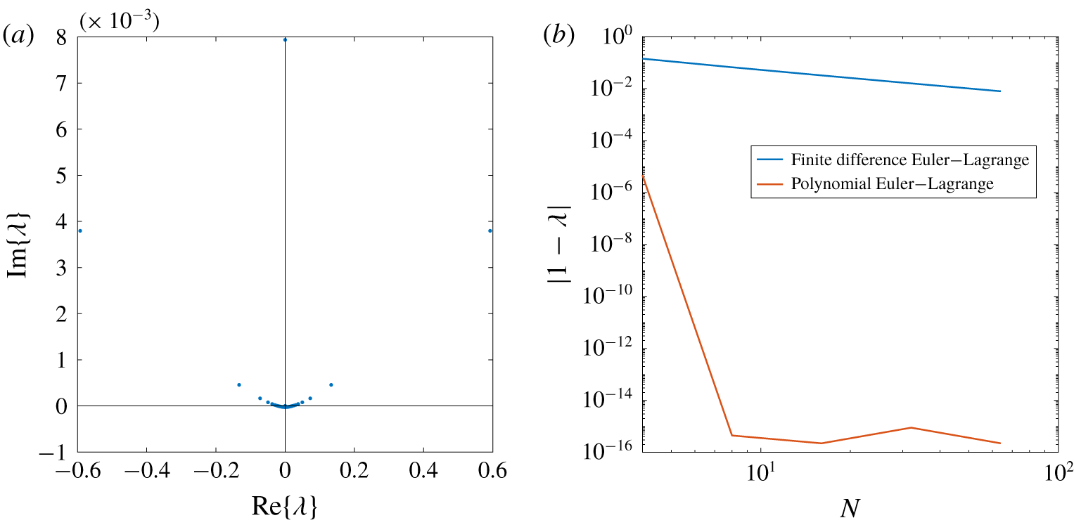
 $\bar{u}(z)=(z/H)^{2}$ yields a full set of complex eigenvalues, where the complex parts are non-trivial and do not diminish with increasing resolution. As an example, we computed the eigenvalues for
 $S(z)=1$,
 $H=1$,
 $\bar{u}(z)=z^{2}/2$ at
 $k_{x}=1$,
 $k_{y}=0$ with 128 grid points; these are plotted in figure 1(a). The eigenvalues all have a non-trivial complex component. The complex part does decrease as the resolution is increased, but slowly: doubling the resolution to 256 points reduces the size of the spurious complex component by a factor of two. Eigenvalues of the continuous problem must all be real, so it is evident that the finite difference method is unreliable here.
(a) Eigenvalues  $\unicode[STIX]{x1D706}$ computed from a finite-difference discretization of the Euler–Lagrange equations (2.9)–(2.11); the number of grid points is 128 and eigenvalues are plotted in the complex plane. (b) Absolute error in the largest instantaneous growth rate
 $\unicode[STIX]{x1D706}$ in the Eady problem for
 $k_{x}=1$,
 $k_{y}=0$ and
 $r=0$ computed by (i) discretizing the continuous QG equations (2.1) and then finding optimals (blue) and (ii) optimizing the Lagrangian of the continuous problem over a subspace of polynomials. In the abscissa for method (i)
 $N$ refers to the number of grid points, while for method (ii)
 $N-1$ is the degree of the polynomials.

Rather than develop an alternate discretization of the Euler–Lagrange equations, we return to the Lagrangian itself (2.6). The Euler–Lagrange equations describe stationary points of the Lagrangian over an infinite-dimensional space (e.g.  $\hat{\unicode[STIX]{x1D713}}_{\boldsymbol{k}}\in C^{2}([0,H])$), and we discretize the problem by restricting attention to a finite-dimensional subspace, specifically polynomials of degree at most
 $N-1$. Finding stationary points of the Lagrangian over this finite-dimensional subspace is straightforward and is guaranteed to produce real eigenvalues
 $\unicode[STIX]{x1D706}$ (which are also Lagrange multipliers); convergence to true values can be monitored by increasing
 $N$.
We use the Legendre polynomial basis,  $\{P_{n}(z)\}_{n=0}^{\infty }$, for the space of polynomials on
 $z\in [0,H]$, so that
 $$\begin{eqnarray}\hat{\unicode[STIX]{x1D713}}_{\boldsymbol{k}}=\mathop{\sum }_{n=0}^{N-1}c_{n}P_{n}(z).\end{eqnarray}$$
Inserting this into  ${\hat{G}}_{\boldsymbol{k}}$ yields
 $$\begin{eqnarray}\displaystyle {\hat{G}}_{\boldsymbol{k}}[\hat{\unicode[STIX]{x1D713}}_{\boldsymbol{k}}] & = & \displaystyle \mathop{\sum }_{n=0}^{N-1}\mathop{\sum }_{m=0}^{N-1}\left[k_{x}\text{Im}\{c_{n}^{\ast }c_{m}\}\int _{0}^{H}\left(S(z)\frac{\text{d}\bar{u}}{\text{d}z}\right)P_{n}(z)P_{m}^{\prime }(z)\,\text{d}z-rk^{2}c_{n}^{\ast }c_{m}P_{n}(0)P_{m}(0)\right]\nonumber\\ \displaystyle & = & \displaystyle \frac{1}{2}\boldsymbol{c}^{\ast }\unicode[STIX]{x1D642}\boldsymbol{c},\end{eqnarray}$$
where  $P_{n}^{\prime }(z)=\text{d}P_{n}(z)/\text{d}z$,
 $\boldsymbol{c}$ is the vector of coefficients
 $c_{n}$ and
 $$\begin{eqnarray}\unicode[STIX]{x1D642}_{n,m}=-2rk^{2}(-1)^{n+m}+\text{i}k_{x}\int _{0}^{H}\left(S(z)\frac{\text{d}\bar{u}}{\text{d}z}\right)(P_{m}(z)P_{n}^{\prime }(z)-P_{n}(z)P_{m}^{\prime }(z))\,\text{d}z.\end{eqnarray}$$
The above uses the Legendre polynomial normalization convention that  $P_{n}(0)=(-1)^{n}$; we also use the convenient but unconventional indexing for the matrix
 $\unicode[STIX]{x1D642}$ starting at
 $0$ rather than 1. Inserting the polynomial into
 $\hat{E}_{\boldsymbol{k}}$ yields
 $$\begin{eqnarray}\displaystyle \hat{E}_{\boldsymbol{k}}[\hat{\unicode[STIX]{x1D713}}_{\boldsymbol{k}}] & = & \displaystyle \frac{1}{2}\mathop{\sum }_{n=0}^{N-1}\mathop{\sum }_{m=0}^{N-1}c_{n}^{\ast }c_{m}\int _{0}^{H}k^{2}P_{n}(z)P_{m}(z)+S(z)P_{n}^{\prime }(z)P_{m}^{\prime }(z)\,\text{d}z\nonumber\\ \displaystyle & = & \displaystyle \frac{1}{2}\boldsymbol{c}^{\ast }\unicode[STIX]{x1D640}\boldsymbol{c},\end{eqnarray}$$
where
 $$\begin{eqnarray}\unicode[STIX]{x1D640}_{n,m}=\frac{Hk^{2}}{2n+1}\unicode[STIX]{x1D6FF}_{nm}+\int _{0}^{H}S(z)P_{n}^{\prime }(z)P_{m}^{\prime }(z)\,\text{d}z\end{eqnarray}$$
where  $\unicode[STIX]{x1D6FF}_{nm}$ is the Kronecker delta, and the indexing again starts at 0 instead of 1. The Lagrangian restricted to this finite-dimensional subspace thus takes the following form
 $$\begin{eqnarray}\hat{I} _{\boldsymbol{k}}[\hat{\unicode[STIX]{x1D713}}_{\boldsymbol{k}}]={\textstyle \frac{1}{2}}\boldsymbol{c}^{\ast }\unicode[STIX]{x1D642}\boldsymbol{c}-\unicode[STIX]{x1D706}{\textstyle \frac{1}{2}}\boldsymbol{c}^{\ast }\unicode[STIX]{x1D640}\boldsymbol{c}.\end{eqnarray}$$
Critical points of the Lagrangian are solutions of the generalized eigenvalue problem
 $$\begin{eqnarray}\unicode[STIX]{x1D642}\boldsymbol{c}=\unicode[STIX]{x1D706}\unicode[STIX]{x1D640}\boldsymbol{c}.\end{eqnarray}$$
Both matrices are Hermitian, while the matrix  $\unicode[STIX]{x1D640}$ is positive definite. As a result, a full set of
 $N$ real eigenvalues is guaranteed to exist. Matlab scripts to construct the matrices
 $\unicode[STIX]{x1D642}$ and
 $\unicode[STIX]{x1D640}$ are included in the supplementary material, available at https://doi.org/10.1017/jfm.2019.969.
To validate the spectral discretization described above we compute solutions to the inviscid Eady problem at  $k_{x}=1$,
 $k_{y}=0$ with
 $S(z)=1$,
 $H=1$ and
 $\bar{u}(z)=z$. The absolute error in the maximal eigenvalue is shown in red as a function of
 $N$ in figure 1(b). The error decreases to machine precision by
 $N=8$. Results at different wavenumbers are qualitatively similar, although eigenvalues at larger
 $k_{x}$ do require higher resolution because they exhibit finer vertical structure, as described in the exact analytical solutions.
A natural alternative to the Legendre polynomials is the well-known baroclinic mode basis (Pedlosky Reference Pedlosky1987, § 6.12). Unfortunately, these basis functions set  $\unicode[STIX]{x2202}_{z}\unicode[STIX]{x1D713}=0$ at the surfaces, which makes them converge much more slowly than polynomials for functions that do not satisfy this condition, including the exact instantaneous optimals of the Eady problem. Furthermore, they are computationally inconvenient, and except for special choices of
 $N^{2}(z)$ they are not known analytically.
3.2 Optimizing the discrete problem
The foregoing section starts with the continuous equations describing instantaneous optimals and discretizes them with a spectral method. As an alternative one can discretize the linear QG equations (2.1) and then seek instantaneous optimals of the discretized model. The standard second-order finite difference discretization of the continuously stratified QG system is described in a variety of places, including Pedlosky (Reference Pedlosky1987, §§ 6.16 and 6.18) and Vallis (Reference Vallis2006, § 5.4); the specific details used here are the same as those in appendix B of Watwood et al. (Reference Watwood, Grooms, Julien and Smith2019). The linear discrete system takes the form
 $$\begin{eqnarray}\frac{\text{d}}{\text{d}t}\unicode[STIX]{x1D648}\boldsymbol{x}=\unicode[STIX]{x1D646}\boldsymbol{x},\end{eqnarray}$$
where the entries of  $\boldsymbol{x}$ are values of
 $\hat{\unicode[STIX]{x1D713}}_{\boldsymbol{k}}$ at the centre of
 $N$ cells from
 $z=0$ to
 $z=H$. The matrix
 $\unicode[STIX]{x1D648}$ is real and symmetric (for an equispaced grid). Code to generate the matrices
 $\unicode[STIX]{x1D648}$ and
 $\unicode[STIX]{x1D646}$ is publicly available (Watwood & Grooms Reference Watwood and Grooms2019). The energy is
 $E=H\boldsymbol{x}^{\ast }\unicode[STIX]{x1D648}\boldsymbol{x}/(2N)$, and energy evolution is
 $$\begin{eqnarray}\frac{\text{d}E}{\text{d}t}=H\boldsymbol{x}^{\ast }\left(\frac{\unicode[STIX]{x1D646}^{\ast }+\unicode[STIX]{x1D646}}{2N}\right)\boldsymbol{x}.\end{eqnarray}$$
Configurations of  $\boldsymbol{x}$ that optimize the instantaneous growth rate of energy subject to the constraint
 $E=1$ are eigenvectors of the generalized eigenvalue problem
 $$\begin{eqnarray}(\unicode[STIX]{x1D646}^{\ast }+\unicode[STIX]{x1D646})\boldsymbol{x}=\unicode[STIX]{x1D706}\unicode[STIX]{x1D648}\boldsymbol{x}.\end{eqnarray}$$
The discretization is validated by computing solutions to the inviscid Eady problem at  $k_{x}=1$,
 $k_{y}=0$ with
 $S(z)=1$,
 $H=1$ and
 $\bar{u}(z)=z$. The absolute error in the maximal eigenvalue is shown in blue as a function of
 $N$ in figure 1(b). The error decreases algebraically, and far more slowly than the spectral discretization described in the preceding section: with
 $N=64$ the finite-difference method is still less accurate than the spectral method with
 $N=4$.
3.3 Numerical results
Both of the numerical methods described above were verified to be accurate in the Eady problem. The spectral method is used in all cases with  $N=64$, with exceptions noted. This section describes numerical results for two different configurations of shear. One configuration, the Phillips-type shear, corresponds to two-layer type behaviour following on the work of Phillips (Reference Phillips1954). The Phillips-type shear consists of a single baroclinic mode with zero shear at the surfaces, and baroclinic instability is related to the fact that the mean potential vorticity gradient
 $\unicode[STIX]{x2202}_{y}\bar{q}$ changes sign once in the interior of the fluid. The second configuration, the Charney-type shear, has a constant mean potential vorticity gradient in the interior of the fluid
 $\unicode[STIX]{x2202}_{y}\bar{q}=-1$ that interacts with shear at the surface to generate instability. The Charney-type set-up is associated with surface-intensified nonlinear dynamics and with increased small-scale energy at the upper surface (Capet et al. Reference Capet, Roullet, Klein and Maze2016). These two types of shear profile are qualitatively representative of the mean shear profiles that drive baroclinic instability throughout the world oceans (Tulloch et al. Reference Tulloch, Marshall, Hill and Smith2011). In both cases we set
 $S(z)=1$ and
 $H=1$. Surface-intensified stratification would be more realistic, but the integrals in (3.4) and (3.6) would no longer be analytically tractable. The two shear profiles investigated here are
 $$\begin{eqnarray}\displaystyle & \displaystyle \text{Phillips-type: }\bar{u}(z)={\textstyle \frac{1}{2}}(-1+6z^{2}-4z^{3}) & \displaystyle\end{eqnarray}$$
 $$\begin{eqnarray}\displaystyle & \displaystyle \text{Charney-type: }\bar{u}(z)=\frac{z^{2}}{2}. & \displaystyle\end{eqnarray}$$
The standard Phillips-type profile (which is a first baroclinic mode) has the form  $-\text{cos}(\unicode[STIX]{x03C0}z)/\unicode[STIX]{x03C0}$; a polynomial mean shear was chosen here since it is qualitatively similar to but more convenient numerically than the cosine profile.
The classical Charney problem is posed in a semi-infinite domain, and is identical to the Eady problem except for the inclusion of a planetary vorticity gradient  $\unicode[STIX]{x1D6FD}$. Although
 $\unicode[STIX]{x1D6FD}$ is absent from the Lagrangian, a semi-infinite domain constitutes a significant change, and caution should be exercised before extrapolating the current results to the classical Charney problem.
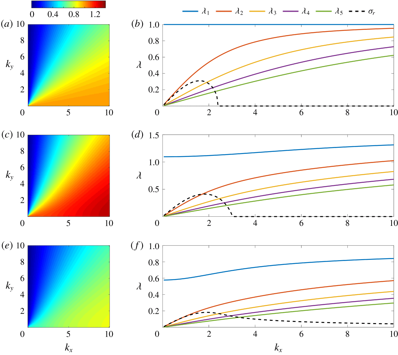
(a,c,e) Largest eigenvalue  $\unicode[STIX]{x1D706}$ of the Euler–Lagrange equations as a function of
 $k_{x}$ and
 $k_{y}$ for the Eady problem (a,b), the Phillips-type problem (c,d) and the Charney-type problem (e,f). (b,d,f) The five largest eigenvalues
 $\unicode[STIX]{x1D706}_{1}>\unicode[STIX]{x1D706}_{2}>\cdots >\unicode[STIX]{x1D706}_{5}$ (solid; coloured), along with the growth rate
 $\unicode[STIX]{x1D70E}_{r}$ of exponentially growing solutions for the corresponding linear stability problem (dashed; black). Solutions computed using polynomials of degree
 $N-1=63$, with
 $r=0$ (inviscid).

Figure 2 shows numerical results on the instantaneous growth rates  $\unicode[STIX]{x1D706}$ for all three problems with
 $r=0$: Eady (a,b), Phillips type (c,d) and Charney type (e,f). Panels (a,c,e) show the most positive eigenvalue
 $\unicode[STIX]{x1D706}$ as a function of wavenumber. Panels (b,d,f) show the five most positive eigenvalues
 $\unicode[STIX]{x1D706}_{1}>\cdots >\unicode[STIX]{x1D706}_{5}$ as a function of
 $k_{x}$ for
 $k_{y}=0$, together with the growth rate
 $\unicode[STIX]{x1D70E}_{r}$ of the fastest-growing mode of the linear stability problem. The behaviour of the three cases is remarkably similar. Growth rates are maximized on the
 $k_{y}=0$ axis, where they are nearly constant. (At larger
 $k_{x}$ with
 $k_{y}=0$ the largest growth rates limit towards a constant value; not shown.) At large scales (small
 $k_{x}$) the largest eigenvalue dominates while all the others approach zero.
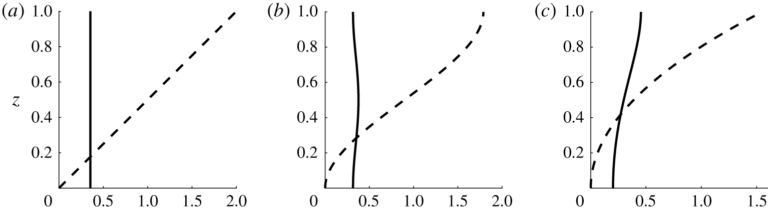
Figure 3 shows numerical results on the vertical structure of the eigenfunction  $\hat{\unicode[STIX]{x1D713}}_{\boldsymbol{k}}(z)$ associated with the largest eigenvalue at
 $k_{x}=2$,
 $k_{y}=0$ with
 $r=0$. The differences between the three problems are more evident here than in their growth rates. The Eady problem has the simple vertical structure proportional to
 $\text{e}^{\text{i}kz}$, as predicted by the analytical solution. In the Phillips-type problem there is no mean shear on the boundary, and the eigenfunctions are required to match this behaviour; the energy growth (first term on the right-hand side of (2.2)) is maximized in mid-layer, where the mean shear is also maximized. In the Charney-type problem there is no mean shear at the lower boundary, and the mean shear is maximized at the upper boundary. The eigenfunctions also have no shear at the lower boundary, and they are surface intensified. In all three problems eigenfunctions corresponding to smaller eigenvalues or to larger wavenumbers
 $k_{x}$ have finer vertical structure (not shown).
Amplitude (solid) and phase (dashed) parts of the optimal perturbations  $\hat{\unicode[STIX]{x1D713}}_{\boldsymbol{k}}$ as a function of
 $z$ at
 $k_{x}=2$,
 $k_{y}=0$ with
 $r=0$ for the Eady (a), Phillips-type (b) and Charney-type (c) problems. Solutions computed with polynomials of degree
 $N-1=63$.

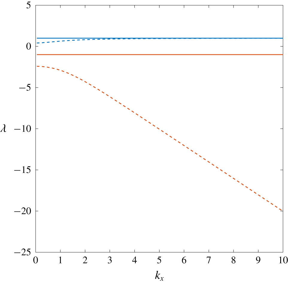
The effect of linear Ekman friction on the exponentially growing modes of linear stability theory is markedly different from the simpler intuitive effect of potential vorticity diffusion (Holopainen Reference Holopainen1961; Barcilon Reference Barcilon1964; Williams & Robinson Reference Williams and Robinson1974). To investigate the effect of friction we compute results with  $r=0.5$. Eigenvalues
 $\unicode[STIX]{x1D706}$ as a function of
 $k_{x}$ for the Eady problem with
 $k_{y}=0$ are shown in figure 4, together with the inviscid results
 $r=0$, for comparison. The most positive and most negative eigenvalues for the inviscid Eady problem are
 $\unicode[STIX]{x1D706}=1$ and
 $-1$, respectively; these are solid lines in figure 4. The most positive and most negative eigenvalues for the Eady problem with
 $r=0.5$ are shown as dashed lines. Ekman friction only has a significant impact on the fastest positive growth rate for eigenfunctions with large horizontal scale (small
 $k_{x}$). These growth rates are reduced, though not to zero, presumably because the associated eigenfunctions are nearly barotropic. In contrast, the fastest-decaying eigenvalues are all strongly impacted by Ekman friction. The associated eigenfunctions have a structure that optimizes the decay rate, which increases linearly with
 $k_{x}$. Results for the Phillips-type and Charney-type problems are qualitatively similar (not shown).
Most-positive and most-negative eigenvalues  $\unicode[STIX]{x1D706}$ for the Eady problem as a function of
 $k_{x}$ with
 $k_{y}=0$ for
 $r=0$ (solid) and
 $r=0.5$ (dashed). The blue lines show the most-positive eigenvalues while the red lines show the most negative. Solutions computed with polynomials of degree
 $N-1=63$. Results for the Charney- and Phillips-type problems are similar (not shown).

4 Discussion
The injection, transfer and ultimate dissipation of energy is an organizing principle in the study of forced–dissipative turbulence. Energy injection via extraction from the background mean flow in quasigeostrophic turbulence forced by baroclinic shear is associated with a quadratic term in the energy budget. This quadratic term can be diagonalized by a basis of eigenfunctions associated with real eigenvalues. Energy injection in quasigeostrophic turbulence forced by baroclinic shear can therefore be associated with excitation and growth of eigenfunctions associated with positive eigenvalues. These eigenfunctions are related to the instantaneous optimal perturbations of non-normal linear stability theory, and are generically referred to here as instantaneous optimals. But the topic here is strongly nonlinear quasigeostrophic turbulence, which is significantly different from the dynamics of subcritical transition in viscous shear flows, where non-normal linear behaviour is well known (Schmid & Henningson Reference Schmid and Henningson2001).
The partitioning of this energy into kinetic and available potential energy and its transfer between forms and between horizontal scales is a complex subject that has been primarily studied in the significantly simpler two-layer model (Salmon Reference Salmon1978; Fu & Flierl Reference Fu and Flierl1980; Haidvogel & Held Reference Haidvogel and Held1980; Scott & Arbic Reference Scott and Arbic2007). In both the two-layer model and in models with higher vertical resolution there is a net energy input to the system over a range of scales larger than the deformation radius in the form of eddy available potential energy (see, e.g. Grooms & Majda Reference Grooms and Majda2014, figure 3d), which is also the range of scales where there are exponentially growing modes of the linear stability problem (Smith & Vallis Reference Smith and Vallis2002; Roullet et al. Reference Roullet, McWilliams, Capet and Molemaker2012; Capet et al. Reference Capet, Roullet, Klein and Maze2016). The potential energy then cascades downscale; near the deformation radius it is converted to eddy kinetic energy, which then cascades to larger scales where it is dissipated via friction. To calculate the actual rate of change of energy at a given wavenumber due to interaction with the mean flow and friction, one resolves the vertical structure at that wavenumber into a sum of instantaneous optimal eigenfunctions. The total energy growth rate is then obtained by summing over the energy in each eigenfunction multiplied by the growth rate associated with that eigenfunction. Our results are broadly consistent with the simulated phenomenology of baroclinic turbulence in the sense that by multiplying the energy spectrum by nearly flat eigenvalues  $\unicode[STIX]{x1D706}$, one obtains an energy injection spectrum concentrated at large scales. This is not completely satisfactory though, because the shape of the energy spectrum presumably depends on the structure of the energy injection and vice versa. Our analysis indicates that energy injection is possible at all horizontal scales, so some reconciliation with the observed confinement of energy injection to a limited range of horizontal scales larger than the deformation radius is needed.
To frame the following discussion, write the fluid system in the following generic form
 $$\begin{eqnarray}\unicode[STIX]{x2202}_{t}u={\mathcal{L}}[u]+{\mathcal{B}}[u,u],\end{eqnarray}$$
where  $u$ generically denotes the flow variables (not the velocity
 $u=-\unicode[STIX]{x2202}_{x}\unicode[STIX]{x1D713}$ of the previous sections),
 ${\mathcal{L}}$ is a linear operator including interaction of the flow with the background mean state and
 ${\mathcal{B}}$ is a bilinear nonlinear advection operator. We can further assume the existence of an energy inner product
 $E=\langle u,u\rangle /2$, and we can decompose the linear term
 ${\mathcal{L}}$ into a piece
 ${\mathcal{L}}_{S}$ that is self-adjoint with respect to the energy inner product, and a piece
 ${\mathcal{L}}_{A}$ that is skew–adjoint with respect to the energy inner product. The eigenvalues and eigenfunctions of the operator
 ${\mathcal{L}}_{S}$ are the growth rates and instantaneous optimals studied in the previous sections.
In the QG problem the flow variable is  $\unicode[STIX]{x1D713}$, the energy inner product is
 $E=\langle \unicode[STIX]{x1D713},\unicode[STIX]{x1D713}\rangle /2$ defined by (2.3), and
 $\langle \unicode[STIX]{x1D713},{\mathcal{L}}\unicode[STIX]{x1D713}\rangle$ is
 $\text{d}E/\text{d}t$ as defined by (2.2). In the QG problem
 ${\mathcal{L}}$ has constant coefficients with respect to the horizontal coordinates
 $x$ and
 $y$, and therefore does not transfer energy between horizontal wavenumbers; only the quadratic nonlinearity transfers energy between horizontal wavenumbers via triad interactions. On the other hand, the nonlinearity in the QG equations does not lead to nonlinear self-interaction at a single wavenumber because
 $\boldsymbol{u}\boldsymbol{\cdot }\unicode[STIX]{x1D735}q=0$ when
 $\boldsymbol{u}$ and
 $q$ are both proportional to
 $\text{e}^{\text{i}(k_{x}x+k_{y}y)}$. In a turbulent setting the nonlinear term will guarantee excitation of all modes, so instantaneous energy growth is not only possible at all scales, it is unavoidable. How can this be reconciled with the evident lack of net energy injection at small scales in simulations of quasigeostrophic turbulence? We conjecture that the answer lies in the role of the skew–adjoint linear operator
 ${\mathcal{L}}_{A}$. This operator is not able to transfer energy between wavenumbers, but it can transfer energy from growing eigenfunctions of
 ${\mathcal{L}}_{S}$ to decaying ones. In fact, at wavenumbers where the operator
 ${\mathcal{L}}$ has no eigenvalues with positive real part it is possible in principle that there is zero net (or sustained) energy growth because of transfer from growing modes of
 ${\mathcal{L}}_{S}$ to decaying ones by
 ${\mathcal{L}}_{A}$. However, if the operator
 ${\mathcal{L}}$ has an eigenvalue with positive real part for some wavenumber then sustained growth at that wavenumber is unavoidable and must be matched by nonlinear transfer to other wavenumbers. This conjecture makes a connection to linear modal stability theory without relying on any assumptions of linearity, and is consistent with the observed lack of energy injection at small horizontal scales in problems like the Eady and Phillips problems where there are no linearly unstable modes at small scales.
To illustrate this mechanism we run simulations of the full QG dynamics using the standard equispaced finite-difference approximation in  $z$, starting from an initial condition that is the optimal perturbation of the finite difference model at wavenumber
 $k_{x}=5$,
 $k_{y}=0$. Simulations are run for all three canonical problems from the preceding section. We solve the inviscid dynamics (
 $r=0$) with
 $N=256$ vertical levels, with constant stratification
 $S(z)=1$ and with
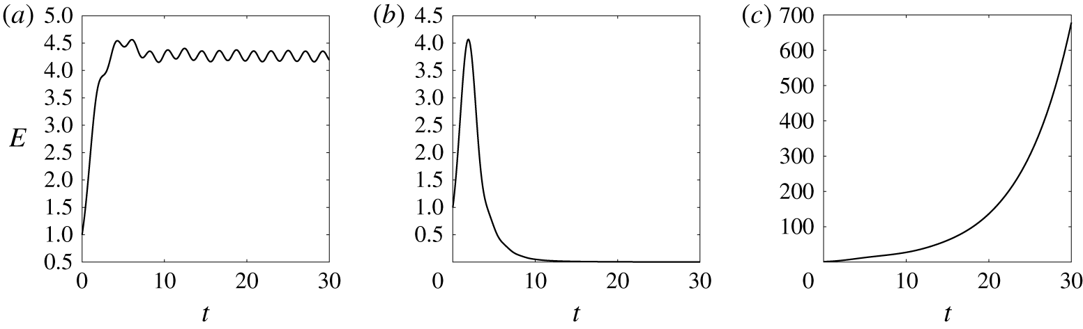
 $H=1$. Since the initial condition consists of a single horizontal wavenumber the nonlinearity is exactly zero for all time, and the dynamics reduces to linear. The time evolution of the energy, starting from unity, is shown in figure 5 for all three simulations.
Energy as a function of time for simulations at  $k_{x}=5$,
 $k_{y}=0$,
 $r=0$, initialized with the optimal perturbation for the Eady (a), Phillips-type (b) and Charney-type (c) problems.

In the Eady problem the energy grows transiently and then sets up a regular oscillation with no further net growth. (With non-zero Ekman friction the energy would eventually decay to zero.) In the Phillips-type problem there is large initial transient growth followed by decay towards zero. In the Charney-type problem the initial condition has a non-zero component in the direction of a linearly unstable mode, and the energy eventually grows exponentially. In the Eady and Phillips-type problems transient growth occurs as the flow extracts energy from the large-scale background, but there is no sustained energy growth. Instead, there is transient decay where the flow returns energy to the background. In the presence of friction some of this transient decay would be associated with friction rather than a return of energy to the background. This behaviour, where the flow at small scales transiently extracts energy from the background flow and then either returns it to the background flow or dissipates it frictionally is consistent with the standard theory of QG turbulence that expects no net energy transfer across horizontal scales at scales smaller than the deformation radius (Charney Reference Charney1971).
Having the small-scale flow transition between extracting energy from the large scales and then returning that energy to the large scales is also connected to the concept of energetic backscatter – transient transfer of energy from small to large scales. Backscatter in idealized ocean models accounts in part for large-scale variability (Kitsios, Frederiksen & Zidikheri Reference Kitsios, Frederiksen and Zidikheri2013), and the development of parameterizations of kinetic energy backscatter for ocean models is a topic of current research (e.g. Kitsios et al. Reference Kitsios, Frederiksen and Zidikheri2013; Jansen & Held Reference Jansen and Held2014; Chen, Barham & Grooms Reference Chen, Barham and Grooms2018). The backscatter associated with linear inviscid decay at small scales as seen here is in the form of potential energy while the aforementioned studies address kinetic energy backscatter. The vertical structure of decaying perturbations could perhaps be used to inform parameterizations of potential energy backscatter within the framework of Grooms (Reference Grooms2016) and Grooms & Kleiber (Reference Grooms and Kleiber2019).
5 Conclusions
The goal of this study is to elucidate the process whereby eddies extract energy from a steady background baroclinic shear in QG turbulence, bridging the gap between linear theory and fully nonlinear dynamics. The term in the eddy energy budget that corresponds to extraction of energy from the background shear is quadratic in the eddy variables and can be diagonalized by an orthonormal basis of eigenfunctions. The associated eigenvalues are the instantaneous energy growth rates associated with each eigenfunction. Any flow configuration can therefore be resolved into a sum of eigenfunctions, each of which is instantaneously extracting energy from the mean or returning energy to the mean. We begin by deriving Euler–Lagrange equations describing the eigenfunctions and eigenvalues in continuously stratified QG dynamics. An exact analytical solution is found for the inviscid Eady problem showing that instantaneous energy growth is possible at all horizontal wavenumbers, and among perturbations with no variation in the  $y$ direction (perpendicular to the background velocity) the fastest-growing ones all have the same growth rate independent of horizontal scale. A spectral numerical method is formulated to compute eigenfunctions and growth rates for vertically varying shear and stratification profiles. We compute eigenvalues for the Eady problem and for a Phillips-type and a Charney-type problem. The Phillips-type problem has no mean shear at the upper and lower surfaces with a mean potential vorticity gradient that changes sign in the interior, and the Charney-type problem has a constant potential vorticity gradient that interacts with shear at the upper surface. In all experiments the stratification
 $N^{2}(z)$ is constant, though the results may extend qualitatively to more realistic surface-intensified stratification. The computed eigenvalues for Phillips-type and Charney-type background flows are remarkably similar to the Eady results, though the eigenfunctions themselves are different. The amplitude of the growing eigenfunctions is concentrated in regions of high shear; in the Charney-type problem they are surface intensified and in the Phillips-type problem they are intensified in the middle of the layer. Ekman friction reduces growth rates at large scales and also leads to a set of eigenfunctions associated with rapid decay, though it has minimal effect on growth at small scales.
Our analytical results show that instantaneous growth is possible at all scales, unlike modal linear stability theory where growth at small scales only occurs in Charney-type problems where an internal potential vorticity gradient interacts with shear at the boundary. In fully nonlinear turbulence triad interactions guarantee non-zero excitation of all Fourier modes, which means that instantaneous growth is not only possible at all scales, it is unavoidable. This needs to be reconciled with the phenomenology of QG turbulence, where sustained extraction of energy from the background mean flow is not observed at small scales, except in Charney-type problems (Smith & Vallis Reference Smith and Vallis2002; Roullet et al. Reference Roullet, McWilliams, Capet and Molemaker2012; Capet et al. Reference Capet, Roullet, Klein and Maze2016). We propose that the transient growth of some eigenfunctions at small scales is matched by transient decay of other eigenfunctions at the same scales, with transfer between them mediated by the skew–adjoint part of the linear operator. The plausibility of this hypothesis is supported by linear simulations where an initial phase of transient growth is either followed by transient decay in the Phillips-type problem, or where it transitions to steady oscillation in the Eady problem. The simulations are inviscid, demonstrating that the mechanism can work without having to match growth by frictional dissipation; the inclusion of frictional dissipation would not change the overall hypothesis though. This hypothesis predicts that Charney-type problems must exhibit sustained energy extraction from the mean flow at all scales, although the rate of extraction at small scales should be weak because of the low energy at small scales. This energy extraction has to be matched by nonlinear transfer to scales where the energy decays, either by frictional processes or by backscatter of energy to the large-scale mean flow.
Acknowledgements
We are grateful to N. Rodriguez for suggesting to optimize the Lagrangian over a finite-dimensional subspace rather than directly discretize the Euler–Lagrange equations. W.B. is supported by US National Science Foundation grant DMS 1407340. This work is partially supported by US National Science Foundation grant OCE 1736708.
Declaration of interests
The authors report no conflict of interest.
Supplementary material
Supplementary material is available at https://doi.org/10.1017/jfm.2019.969.
Appendix A
The Euler–Lagrange equations (2.9)–(2.11) are derived in this appendix. Let  $\unicode[STIX]{x1D719}$ represent a perturbation of
 $\hat{\unicode[STIX]{x1D713}}_{\boldsymbol{k}}$. Inserting
 $\hat{\unicode[STIX]{x1D713}}_{\boldsymbol{k}}+\unicode[STIX]{x1D719}$ into
 $\hat{I} _{\boldsymbol{k}}$ and retaining linear terms in
 $\unicode[STIX]{x1D719}$, we obtain,
 $$\begin{eqnarray}\displaystyle & & \displaystyle -\displaystyle \frac{\text{i}k_{x}}{2}\int _{0}^{1}\left(S(z)\frac{\text{d}\bar{u}}{\text{d}z}\right)[\hat{\unicode[STIX]{x1D713}}_{\boldsymbol{k}}^{\ast }\unicode[STIX]{x2202}_{z}\unicode[STIX]{x1D719}+\unicode[STIX]{x1D719}^{\ast }\unicode[STIX]{x2202}_{z}\hat{\unicode[STIX]{x1D713}}_{\boldsymbol{k}}-\hat{\unicode[STIX]{x1D713}}_{\boldsymbol{k}}\unicode[STIX]{x2202}_{z}\unicode[STIX]{x1D719}^{\ast }-\unicode[STIX]{x1D719}\unicode[STIX]{x2202}_{z}\hat{\unicode[STIX]{x1D713}}_{\boldsymbol{k}}^{\ast }]\,\text{d}z\nonumber\\ \displaystyle & & \displaystyle \quad \displaystyle -\frac{\unicode[STIX]{x1D706}}{2}\int _{0}^{1}k^{2}(\unicode[STIX]{x1D719}\hat{\unicode[STIX]{x1D713}}_{\boldsymbol{k}}^{\ast }+\hat{\unicode[STIX]{x1D713}}_{\boldsymbol{k}}\unicode[STIX]{x1D719}^{\ast })+S(z)[\unicode[STIX]{x2202}_{z}\unicode[STIX]{x1D719}\unicode[STIX]{x2202}_{z}\hat{\unicode[STIX]{x1D713}}_{\boldsymbol{k}}^{\ast }+\unicode[STIX]{x2202}_{z}\hat{\unicode[STIX]{x1D713}}_{\boldsymbol{k}}\unicode[STIX]{x2202}_{z}\unicode[STIX]{x1D719}^{\ast }]\,\text{d}z\nonumber\\ \displaystyle & & \displaystyle \quad \displaystyle -\,rk^{2}((\unicode[STIX]{x1D719}^{-})^{\ast }\hat{\unicode[STIX]{x1D713}}_{\boldsymbol{k}}^{-}+\unicode[STIX]{x1D719}^{-}(\hat{\unicode[STIX]{x1D713}}_{\boldsymbol{k}}^{-})^{\ast }).\end{eqnarray}$$
Simplifying with integration by parts, we obtain,
 $$\begin{eqnarray}\displaystyle & & \displaystyle \left.\left[-\frac{\text{i}k_{x}}{2}\left(S(z)\frac{\text{d}\bar{u}}{\text{d}z}\right)[\hat{\unicode[STIX]{x1D713}}_{\boldsymbol{k}}^{\ast }\unicode[STIX]{x1D719}-\hat{\unicode[STIX]{x1D713}}_{\boldsymbol{k}}\unicode[STIX]{x1D719}^{\ast }]\right]\right|_{z=0}^{H}\nonumber\\ \displaystyle & & \displaystyle \quad +\,\frac{\text{i}k_{x}}{2}\int _{0}^{1}\unicode[STIX]{x2202}_{y}\bar{q}[\hat{\unicode[STIX]{x1D713}}_{\boldsymbol{k}}\unicode[STIX]{x1D719}^{\ast }-\hat{\unicode[STIX]{x1D713}}_{\boldsymbol{ k}}^{\ast }\unicode[STIX]{x1D719}]+2\left(S(z)\frac{\text{d}\bar{u}}{\text{d}z}\right)[\unicode[STIX]{x1D719}^{\ast }\unicode[STIX]{x2202}_{z}\hat{\unicode[STIX]{x1D713}}_{\boldsymbol{k}}-\unicode[STIX]{x1D719}\unicode[STIX]{x2202}_{z}\hat{\unicode[STIX]{x1D713}}_{\boldsymbol{k}}^{\ast }]\,\text{d}z\nonumber\\ \displaystyle & & \displaystyle \quad -\,\frac{\unicode[STIX]{x1D706}}{2}[S(z)(\unicode[STIX]{x1D719}\unicode[STIX]{x2202}_{z}\hat{\unicode[STIX]{x1D713}}_{\boldsymbol{k}}^{\ast }+\unicode[STIX]{x1D719}^{\ast }\unicode[STIX]{x2202}_{z}\hat{\unicode[STIX]{x1D713}}_{\boldsymbol{k}})]|_{z=0}^{H}\nonumber\\ \displaystyle & & \displaystyle \quad -\,\frac{\unicode[STIX]{x1D706}}{2}\int _{0}^{1}k^{2}(\unicode[STIX]{x1D719}\hat{\unicode[STIX]{x1D713}}_{\boldsymbol{k}}^{\ast }+\hat{\unicode[STIX]{x1D713}}_{\boldsymbol{k}}\unicode[STIX]{x1D719}^{\ast })-\unicode[STIX]{x1D719}\unicode[STIX]{x2202}_{z}(S(z)\unicode[STIX]{x2202}_{z}\hat{\unicode[STIX]{x1D713}}_{\boldsymbol{k}}^{\ast })-\unicode[STIX]{x1D719}^{\ast }\unicode[STIX]{x2202}_{z}(S(z)\unicode[STIX]{x2202}_{z}\hat{\unicode[STIX]{x1D713}}_{\boldsymbol{k}})\,\text{d}z\nonumber\\ \displaystyle & & \displaystyle \quad -\,rk^{2}((\unicode[STIX]{x1D719}^{-})^{\ast }\hat{\unicode[STIX]{x1D713}}_{\boldsymbol{k}}^{-}+\unicode[STIX]{x1D719}^{-}(\hat{\unicode[STIX]{x1D713}}_{\boldsymbol{k}}^{-})^{\ast }).\end{eqnarray}$$
The above uses the following identity relating the mean shear to the mean potential vorticity gradient
 $$\begin{eqnarray}\frac{\text{d}}{\text{d}z}\left(S(z)\frac{\text{d}\bar{u}}{\text{d}z}\right)=-\unicode[STIX]{x2202}_{y}\bar{q}.\end{eqnarray}$$
This simplifies to
 $$\begin{eqnarray}\displaystyle & & \displaystyle \left.\left[k_{x}\left(S(z)\frac{\text{d}\bar{u}}{\text{d}z}\right)\text{Im}\{\hat{\unicode[STIX]{x1D713}}_{\boldsymbol{k}}^{\ast }\unicode[STIX]{x1D719}\}-\unicode[STIX]{x1D706}S(z)\text{Re}\{\unicode[STIX]{x1D719}\unicode[STIX]{x2202}_{z}\hat{\unicode[STIX]{x1D713}}_{\boldsymbol{k}}^{\ast }\}\right]\right|_{z=0}^{1}-2rk^{2}\text{Re}\{(\unicode[STIX]{x1D719}^{-})^{\ast }\hat{\unicode[STIX]{x1D713}}_{\boldsymbol{k}}^{-}\}\nonumber\\ \displaystyle & & \displaystyle \quad -\,k_{x}\int _{0}^{1}\unicode[STIX]{x2202}_{y}\bar{q}\,\text{Im}\{\hat{\unicode[STIX]{x1D713}}_{\boldsymbol{k}}\unicode[STIX]{x1D719}^{\ast }\}+2\left(S(z)\frac{\text{d}\bar{u}}{\text{d}z}\right)\text{Im}\{\unicode[STIX]{x1D719}^{\ast }\unicode[STIX]{x2202}_{z}\hat{\unicode[STIX]{x1D713}}_{\boldsymbol{k}}\}\,\text{d}z\nonumber\\ \displaystyle & & \displaystyle \quad -\,\unicode[STIX]{x1D706}\int _{0}^{1}\text{Re}\{\unicode[STIX]{x1D719}(k^{2}\unicode[STIX]{x1D713}_{\boldsymbol{k}}^{\ast }-(\unicode[STIX]{x2202}_{z}S\unicode[STIX]{x2202}_{z}\unicode[STIX]{x1D713}_{\boldsymbol{k}}^{\ast }))\}\,\text{d}z.\end{eqnarray}$$
Stationary configurations of  $\hat{\unicode[STIX]{x1D713}}_{\boldsymbol{k}}$ are defined to be those for which the above expression is zero for every
 $\unicode[STIX]{x1D719}$, in particular for
 $\unicode[STIX]{x1D719}$ that are zero on the boundaries, which means that the integral and the boundary terms must vanish separately. Thus we have
 $$\begin{eqnarray}\displaystyle & \displaystyle k_{x}\left(S(z)\frac{\text{d}\bar{u}}{\text{d}z}\right)\text{Im}\{\hat{\unicode[STIX]{x1D713}}_{\boldsymbol{k}}^{\ast }\unicode[STIX]{x1D719}\}-\unicode[STIX]{x1D706}S(z)\text{Re}\{\unicode[STIX]{x1D719}\unicode[STIX]{x2202}_{z}\hat{\unicode[STIX]{x1D713}}_{\boldsymbol{k}}^{\ast }\}-2rk^{2}\text{Re}\{(\unicode[STIX]{x1D719}^{-})^{\ast }\hat{\unicode[STIX]{x1D713}}_{\boldsymbol{k}}^{-}\}=0\quad \text{at }z=0,\quad & \displaystyle\end{eqnarray}$$
 $$\begin{eqnarray}\displaystyle & \displaystyle k_{x}\left(S(z)\frac{\text{d}\bar{u}}{\text{d}z}\right)\text{Im}\{\hat{\unicode[STIX]{x1D713}}_{\boldsymbol{k}}^{\ast }\unicode[STIX]{x1D719}\}-\unicode[STIX]{x1D706}S(z)\text{Re}\{\unicode[STIX]{x1D719}\unicode[STIX]{x2202}_{z}\hat{\unicode[STIX]{x1D713}}_{\boldsymbol{k}}^{\ast }\}=0\quad \text{at }z=H, & \displaystyle\end{eqnarray}$$
and
 $$\begin{eqnarray}\displaystyle & & \displaystyle -k_{x}\unicode[STIX]{x2202}_{y}\bar{q}\,\text{Im}\{\hat{\unicode[STIX]{x1D713}}_{\boldsymbol{k}}\unicode[STIX]{x1D719}^{\ast }\}+2\left(S(z)\frac{\text{d}\bar{u}}{\text{d}z}\right)\text{Im}\{\unicode[STIX]{x1D719}^{\ast }\unicode[STIX]{x2202}_{z}\hat{\unicode[STIX]{x1D713}}_{\boldsymbol{k}}\}\nonumber\\ \displaystyle & & \displaystyle \quad -\,\unicode[STIX]{x1D706}\text{Re}\{\unicode[STIX]{x1D719}(k^{2}\unicode[STIX]{x1D713}_{\boldsymbol{k}}^{\ast }-\unicode[STIX]{x2202}_{z}(S(z)\unicode[STIX]{x2202}_{z}\unicode[STIX]{x1D713}_{\boldsymbol{k}}^{\ast }))\}=0,\end{eqnarray}$$
for  $z\in (0,H)$. Let
 $\hat{\unicode[STIX]{x1D713}}_{\boldsymbol{k}}=\unicode[STIX]{x1D713}_{r}+\text{i}\unicode[STIX]{x1D713}_{i}$ and
 $\unicode[STIX]{x1D719}=\unicode[STIX]{x1D719}_{r}+\text{i}\unicode[STIX]{x1D719}_{i}$ be the complex expression of
 $\hat{\unicode[STIX]{x1D713}}_{\boldsymbol{k}}$ and
 $\unicode[STIX]{x1D719}$. Then we may write (A 7) as
 $$\begin{eqnarray}\displaystyle & \displaystyle -k_{x}\unicode[STIX]{x2202}_{y}\bar{q}(\unicode[STIX]{x1D719}_{r}\unicode[STIX]{x1D713}_{i}-\unicode[STIX]{x1D719}_{i}\unicode[STIX]{x1D713}_{r})+2k_{x}\left(S(z)\frac{\text{d}\bar{u}}{\text{d}z}\right)(\unicode[STIX]{x1D719}_{r}\unicode[STIX]{x2202}_{z}\unicode[STIX]{x1D713}_{i}-\unicode[STIX]{x1D719}_{i}\unicode[STIX]{x2202}_{z}\unicode[STIX]{x1D713}_{r}) & \displaystyle\end{eqnarray}$$
 $$\begin{eqnarray}\displaystyle & \displaystyle -\unicode[STIX]{x1D706}[\unicode[STIX]{x1D719}_{r}(k^{2}\unicode[STIX]{x1D713}_{r}-\unicode[STIX]{x2202}_{z}(S(z)\unicode[STIX]{x2202}_{z}\unicode[STIX]{x1D713}_{r}))]-\unicode[STIX]{x1D706}[\unicode[STIX]{x1D719}_{i}(k^{2}\unicode[STIX]{x1D713}_{i}-\unicode[STIX]{x2202}_{z}(S(z)\unicode[STIX]{x2202}_{z}\unicode[STIX]{x1D713}_{i}))]=0. & \displaystyle\end{eqnarray}$$
Again, since this has to be true for any  $\unicode[STIX]{x1D719}$, including cases where
 $\unicode[STIX]{x1D719}_{r}=0$ or
 $\unicode[STIX]{x1D719}_{i}=0$. From this follows the system of equations
 $$\begin{eqnarray}\displaystyle & \displaystyle -k_{x}\unicode[STIX]{x2202}_{y}\bar{q}\,\unicode[STIX]{x1D713}_{i}+2k_{x}\left(S(z)\frac{\text{d}\bar{u}}{\text{d}z}\right)\unicode[STIX]{x2202}_{z}\unicode[STIX]{x1D713}_{i}-\unicode[STIX]{x1D706}(k^{2}\unicode[STIX]{x1D713}_{r}-\unicode[STIX]{x2202}_{z}(S(z)\unicode[STIX]{x2202}_{z}\unicode[STIX]{x1D713}_{r}))=0 & \displaystyle\end{eqnarray}$$
 $$\begin{eqnarray}\displaystyle & \displaystyle k_{x}\unicode[STIX]{x2202}_{y}\bar{q}\,\unicode[STIX]{x1D713}_{r}-2k_{x}\left(S(z)\frac{\text{d}\bar{u}}{\text{d}z}\right)\unicode[STIX]{x2202}_{z}\unicode[STIX]{x1D713}_{r}-\unicode[STIX]{x1D706}(k^{2}\unicode[STIX]{x1D713}_{i}-\unicode[STIX]{x2202}_{z}(S(z)\unicode[STIX]{x2202}_{z}\unicode[STIX]{x1D713}_{i}))=0. & \displaystyle\end{eqnarray}$$
Multiplying the second equation by  $\text{i}$ and adding, we get
 $$\begin{eqnarray}-\text{i}k_{x}\unicode[STIX]{x2202}_{y}\bar{q}\,\hat{\unicode[STIX]{x1D713}}_{\boldsymbol{k}}+2\text{i}k_{x}\left(S(z)\frac{\text{d}\bar{u}}{\text{d}z}\right)\unicode[STIX]{x2202}_{z}\hat{\unicode[STIX]{x1D713}}_{\boldsymbol{k}}+\unicode[STIX]{x1D706}(k^{2}\hat{\unicode[STIX]{x1D713}}_{\boldsymbol{ k}}-\unicode[STIX]{x2202}_{z}(S(z)\unicode[STIX]{x2202}_{z}\hat{\unicode[STIX]{x1D713}}_{\boldsymbol{k}}))=0,\quad \text{for }z\in (0,H).\end{eqnarray}$$
This is (2.9). We next return to the boundary conditions. Again splitting into real and imaginary parts, we get
 $$\begin{eqnarray}\displaystyle & & \displaystyle k_{x}\left(S(z)\frac{\text{d}\bar{u}}{\text{d}z}\right)[\unicode[STIX]{x1D713}_{r}\unicode[STIX]{x1D719}_{i}-\unicode[STIX]{x1D713}_{i}\unicode[STIX]{x1D719}_{r}]-\unicode[STIX]{x1D706}S(z)[\unicode[STIX]{x1D719}_{r}\unicode[STIX]{x2202}_{z}\unicode[STIX]{x1D713}_{r}+\unicode[STIX]{x1D719}_{i}\unicode[STIX]{x2202}_{z}\unicode[STIX]{x1D713}_{i}]\nonumber\\ \displaystyle & & \displaystyle \quad -\,rk^{2}(\unicode[STIX]{x1D719}_{r}\unicode[STIX]{x1D713}_{r}+\unicode[STIX]{x1D719}_{i}\unicode[STIX]{x1D713}_{i})=0,\quad \text{for }z=0.\end{eqnarray}$$
 $$\begin{eqnarray}k_{x}\left(S(z)\frac{\text{d}\bar{u}}{\text{d}z}\right)[\unicode[STIX]{x1D713}_{r}\unicode[STIX]{x1D719}_{i}-\unicode[STIX]{x1D713}_{i}\unicode[STIX]{x1D719}_{r}]-\unicode[STIX]{x1D706}S(z)[\unicode[STIX]{x1D719}_{r}\unicode[STIX]{x2202}_{z}\unicode[STIX]{x1D713}_{r}+\unicode[STIX]{x1D719}_{i}\unicode[STIX]{x2202}_{z}\unicode[STIX]{x1D713}_{i}]=0,\quad \text{for }z=H.\end{eqnarray}$$
Alternately setting  $\unicode[STIX]{x1D719}_{r}=0$ and
 $\unicode[STIX]{x1D719}_{i}=0$ gives rise to the equations
 $$\begin{eqnarray}\displaystyle & \displaystyle -k_{x}\left(S(z)\frac{\text{d}\bar{u}}{\text{d}z}\right)\unicode[STIX]{x1D713}_{i}-\unicode[STIX]{x1D706}S(z)\unicode[STIX]{x2202}_{z}\unicode[STIX]{x1D713}_{r}=0\quad \text{and } & \displaystyle\end{eqnarray}$$
 $$\begin{eqnarray}\displaystyle & \displaystyle k_{x}\left(S(z)\frac{\text{d}\bar{u}}{\text{d}z}\right)\unicode[STIX]{x1D713}_{r}-\unicode[STIX]{x1D706}S(z)\unicode[STIX]{x2202}_{z}\unicode[STIX]{x1D713}_{i}=0,\quad \text{for }z=H. & \displaystyle\end{eqnarray}$$
Multiplying the second equation by  $\text{i}$ and adding, we get (2.11)
 $$\begin{eqnarray}\text{i}k_{x}\left(S(z)\frac{\text{d}\bar{u}}{\text{d}z}\right)\hat{\unicode[STIX]{x1D713}}_{\boldsymbol{k}}-\unicode[STIX]{x1D706}S(z)\unicode[STIX]{x2202}_{z}\hat{\unicode[STIX]{x1D713}}_{\boldsymbol{k}}=0,\quad \text{for }z=H.\end{eqnarray}$$
The same process at  $z=0$ gives rise to the equations
 $$\begin{eqnarray}\displaystyle & \displaystyle -k_{x}\left(S(z)\frac{\text{d}\bar{u}}{\text{d}z}\right)\unicode[STIX]{x1D713}_{i}-\unicode[STIX]{x1D706}S(z)\unicode[STIX]{x2202}_{z}\unicode[STIX]{x1D713}_{r}-rk^{2}\unicode[STIX]{x1D713}_{r}=0\quad \text{and } & \displaystyle\end{eqnarray}$$
 $$\begin{eqnarray}\displaystyle & \displaystyle k_{x}\left(S(z)\frac{\text{d}\bar{u}}{\text{d}z}\right)\unicode[STIX]{x1D713}_{r}-\unicode[STIX]{x1D706}S(z)\unicode[STIX]{x2202}_{z}\unicode[STIX]{x1D713}_{i}-rk^{2}\unicode[STIX]{x1D713}_{i}=0,\quad \text{for }z=0. & \displaystyle\end{eqnarray}$$
Multiplying the second equation by  $\text{i}$ and adding, we get (2.10)
 $$\begin{eqnarray}\text{i}k_{x}\left(S(z)\frac{\text{d}\bar{u}}{\text{d}z}\right)\hat{\unicode[STIX]{x1D713}}_{\boldsymbol{k}}-\unicode[STIX]{x1D706}S(z)\unicode[STIX]{x2202}_{z}\hat{\unicode[STIX]{x1D713}}_{\boldsymbol{k}}-2rk^{2}\hat{\unicode[STIX]{x1D713}}_{\boldsymbol{ k}}=0,\quad \text{for }z=0.\end{eqnarray}$$