1. Introduction
Redundant agents are designed to improve the fault tolerance, robustness, and task completion efficiency of a multi-agent system by deploying more agents than are actually needed for the tasks [Reference Prorok1]. It overcomes the problem of failure or performance bottleneck through cooperation and redundant backup between agents.
A swarm is a large-scale collection of autonomous agents that interact with each other and their environment to achieve a common goal through self-organized cooperation [Reference Abdelli, Yachir, Amamra and Khaldi2]. In recent years, with the rapid development of distributed computing technology and the wide application of swarm intelligence systems, the cooperative optimization of redundant agents has gradually become an important research direction in the field of complex system control. The key feature of such systems is to achieve functional redundancy and fault tolerance through super-large-scale agent networks. However, when dealing with such high-dimensional systems, traditional task allocation methods generally face problems such as the high dimension of the decision space and poor scalability. Especially in the dynamic and open environment, there are significant bottlenecks in the real-time performance and resource efficiency of the existing methods, which are difficult to meet the strict requirements of the system for speed and cost. Therefore, a distributed task allocation framework with sub-linear time complexity for dynamic environments has become the key to improving the performance of intelligent swarm systems.
The redundant agent system has shown significant advantages in task allocation [Reference Ramos, Pinto and Haddad3] in various fields. Its deployment overcomes the shortcomings of a single agent system and can perform complex tasks faster than a single agent in a centralized or distributed way [Reference Seenu, Kuppan Chetty, Ramya and Janardhanan4, Reference Raptis and Sullivan5]. In industrial production, redundant agents can ensure that the production line continues to operate even if an agent fails, thus reducing downtime and production losses. In the field of logistics and transportation, redundant agents improve the speed [Reference Prorok1] and fairness [Reference Malencia, Kumar, Pappas and Prorok6] of the distribution of goods by optimizing routes and assigning tasks and reduce operating costs. In the field of unmanned driving and robotics, redundant agents enhance the system’s environmental adaptability and decision-making accuracy by cooperating and sharing information with each other. In addition, in the military and security fields, the application of redundant agents can significantly improve the success rate of task execution and the anti-jamming ability of the system. In conclusion, the introduction of redundant agents not only improves the efficiency and reliability of task allocation in various fields but also provides an important guarantee for the stable operation of the system.
Distributed task allocation is an application of the distributed constraint optimization problem (DCOP). Distributed task allocation refers to the process in which a group of autonomous agents, through local perception, communication, and decision-making, jointly decide how to allocate a set of tasks to the members of the group without a central control node, aiming to optimize one or more global performance indicators such as total completion time, total consumption, system efficiency, etc. This can often be mathematically described as a DCOP. The availability of resources, the requirements of tasks, and other conditions are treated as constraints, while the goal of task allocation is to optimize the objective function [Reference Deng and Chen7]. The variables are controlled by agents, and the communication model is local.
In recent years, researchers have proposed a variety of improved algorithms to solve DCOP. Chen et al. [Reference Chen, He, He and Chen16] proposed a hybrid DCOP algorithm based on the combination of breadth-first search (BFS) and depth-first search (DFS), which introduced a hierarchical boundary and divided all agents into agents based on BFS and agents based on DFS. Detailed experimental results show that the proposed method outperforms some well-known search-based full DCOP algorithms on benchmark problems. Chen et al. [Reference Chen, Deng, Chen, Zhang and He17] mixed search with context-based reasoning and proposed a complete DCOP algorithm, where reasoning utilizes contexts derived from the search process to establish tight lower bounds, while search uses these bounds for efficient pruning, thereby reducing the context of reasoning. Nguyen et al. [Reference Nguyen, Yeoh, Lau and Zivan18] introduced two new sampling-based DCOP algorithms, called sequential distributed gibbs (SD-Gibbs) and parallel distributed gibbs (PD-Gibbs). These two algorithms are able to find better solutions than distributed UCT (DUCT), run faster than DUCT, and solve some large-scale problems that cannot be solved due to memory limitations.
Although the DCOP method provides a theoretical framework for multi-agent cooperative task allocation, it still faces significant challenges in complex dynamic scenarios. Traditional methods are difficult to balance real-time response and global solution quality due to the inherent contradiction between high-dimensional constraint coupling and communication-computation efficiency. The robust modeling ability of heterogeneous resource conflicts and multi-objective priority coupling is insufficient. In addition, in practical scenarios with strong uncertainty, realistic constraints such as communication delay and partial observability further aggravate the imbalance between reliability and real-time performance of the algorithm.
Multi-robot task allocation can be categorized into different classes based on three criteria [Reference Gerkey and Matarić8]. The first criterion is single-task robots (ST) versus multi-task robots (MT). Identifies whether each robot can complete only one or multiple tasks at a time. The second criterion is single-robot task (SR) versus multi-robot task (MR). Identifies whether each task requires only one robot or multiple robots to complete. The third criterion is instantaneous allocation (IA) versus time-extended allocation (TA). It distinguishes between allocating to robots instantaneously or with respect to future allocations without a future allocation plan. This means that each robot is assigned several tasks that must be completed according to a given schedule. According to the above classification, the dynamic task allocation of redundant agents to be solved in this paper is a headcount-only task allocation of ST-MR-IA. It is a model for repeatedly solving static snapshots of an allocation problem in a dynamic environment.
In multi-agent systems, the solutions of task allocation can be divided into several main categories according to different strategies and methods, including market-based methods, behavior-based methods, and optimization-based methods [Reference Seenu, Kuppan Chetty, Ramya and Janardhanan4]. First, market-based methods are inspired by economic principles, where tasks are treated as commodities and agents as bidders. The main idea of distributed market-based methods is that agents exchange and coordinate their bidding information with neighbors, resolve competition conflicts for the same task by comparing bidding values (usually the highest bidder wins the task), and finally reach a consensus on the task-allocation result throughout the system. The consensual-based auction algorithm [Reference Choi, Brunet and How9] is a typical representative of this kind of method. Secondly, optimization-based methods focus on finding the optimal solution for task allocation directly through algorithms. Such methods usually adopt integer linear programming (ILP) [Reference Ghassemi and Chowdhury10], heuristic methods [Reference Yan and Di11], metaheuristic algorithms [Reference Saeedvand, Aghdasi and Baltes12], etc. These algorithms are capable of addressing large-scale and complex optimization problems. However, the main disadvantage of such methods is that most of them are difficult to apply in distributed systems, because they often require centralized decision-making and a large amount of computational resources. For methods that can be applied in a distributed setting after correctly formulating the objectives and constraints (such as mixed-integer linear programming, MILP), their main drawback is that they require consistent performance on all nodes. Finally, behavior-based methods divide task allocation into a series of actions, each of which has a corresponding priority or follows a specific rule. This method focuses on regulating the behavior pattern of the agent and optimizes the completion of the task by determining the execution order of the behavior. Representative algorithms include Alliance [Reference Parker13] and Markov Decision Process [Reference Wu, Dong, Sun and Yu14]. The confidence proxy-driven posterior correction and greedy swapping method (CPPC-GS) proposed in this paper is also a behavior-based method.
Market-based methods in task allocation leverage decentralized auction, contract, and bidding mechanisms to enable self-organized resource coordination in multi-agent systems. Zhang et al. [Reference Zhang, Chen, Wei and Wu26] proposed a new group-oriented adjustable bidding task assignment (GO-ABTA) algorithm to solve the group-oriented two-sided preference matching problem. Grillo et al. [Reference Grillo, Carpin, Recchiuto and Sgorbissa27] introduced the trust mechanism into the auction algorithm to solve the problem of cooperation without knowing each other’s capabilities. Oh et al. [Reference Oh, Kim, Ahn and Choi28] proposed a new market-based decentralized algorithm for the task allocation of multiple Uavs. In particular, a cooperative timing task that cannot be performed by a single vehicle is considered. The baseline algorithm for connected networks is extended to handle time-varying network topologies including isolated subnetworks with local communication range.
Market-based task allocation methods improve the self-organization ability of multi-agent systems through a decentralization mechanism. However, due to the dependence on global information synchronization and high communication frequency, the traditional auction/bidding mechanism has the problems of low negotiation efficiency and intensified resource contention. In addition, most of the existing methods assume that the task-resource mapping relationship is statically divisible and are not robust to task insertion, which limits their reliability in strongly uncertain scenarios.
Optimization-based methods in task allocation have emerged as pivotal tools for addressing complex multi-agent coordination challenges. Liu et al. [Reference Liu, Jing and Hou19] proposed a two-stage centralized unmanned aerial vehicle (UAV) task allocation model based on expectation maximization (EM) clustering and the multi-dimensional knapsack problem (MKP). It is used for the allocation of forest fire reconnaissance tasks. Liu et al. [Reference Liu, Wang, Xu and Liu20] proposed a distributed task allocation method: partitioning tasks into groups to reduce conflicts and communication overhead, employing enhanced ant colony optimization for UAV task assignment, and introducing an inter-cluster adjustment mechanism to improve allocation rates. Zhou et al. [Reference Zhou, Lu, Xu and Wu21] proposed a task allocation method based on the multi-strategy improved dung beetle optimization (MSIDBO) algorithm to solve the fully distributed multi-agent cross-domain cooperative task allocation problem. To address the limitations of the original dung beetle optimization algorithm in solving such problems, four revolutionary strategies are introduced to improve its performance. Martin et al. [Reference Martin, García and Camacho22] proposed an event-MILP-based algorithm to solve the task allocation problem in a robotic sensor network (RSN). The algorithm can be applied to the distributed estimation of the solar irradiance on a parabolic trough thermosolar power plant, which can be used to increase the global efficiency of the plant. Chopra et al. [Reference Chopra, Notarstefano, Rice and Egerstedt23] proposed a distributed version of the Hungarian method to solve the well-known assignment problem. In the context of multirobot applications, all robots cooperatively compute a common assignment that optimizes a given global criterion (e.g., the total distance traveled) within a finite set of local computations and communications over a peer-to-peer network. Notomista et al. [Reference Notomista, Mayya, Emam, Kroninger, Bohannon, Hutchinson and Egerstedt24] developed an energy-aware framework based on a mixed-integer quadratic program (MIQP) for allocating tasks to robots in an online fashion. Furthermore, they presented a novel framework to represent the heterogeneous capabilities of the robots by distinguishing between the features available on the robots and the capabilities enabled by these features. Govoni et al. [Reference Govoni and Cristofaro25] proposed an algorithm that, based on a quadratic program (QP) and local information only, can simultaneously assign the tasks, consistently with the different nature of each robot, and allocate the control efforts while satisfying the constraints on the actuators. The performances of the proposed method had been analyzed by means of a simulation study, considering different scenarios and illustrating also the resilience of the approach with respect to faults.
In general, although numerous studies have been dedicated to improving the real-time performance, fault tolerance, and scalability of centralized methods, these methods still often face severe challenges in high-real-time, strongly uncertain large-scale dynamic scenarios. Similarly, although distributed optimization algorithms reduce communication costs, they often need to trade off convergence speed and global optimality, and many optimization algorithms rely on empirical tuning of parameters and lack convergence theory guarantees. The above problems jointly restrict the application efficiency of relevant methods in harsh practical environments.
Behavior-based methods in task allocation focus on emergent coordination through bio-inspired or social interaction models, such as swarm intelligence and adaptive rules. Yin et al. [Reference Yin, Guo, Su and Wang29] designed a QMIX-based deep transfer reinforcement learning algorithm. The algorithm first compares the target task with the source task in the policy library to find the task with the highest similarity and then migrates the network parameters and stores them in the policy library to accelerate the convergence of the QMIX algorithm. Wang et al. [Reference Wang, Zhu, Guo, Ma and Li30] proposed a distributed emotional robot tracking task allocation algorithm based on self-awareness, which combined cognitive intelligence with emotional intelligence to establish self-awareness of emotional robots. Chen et al. [Reference Chen, Rosolia and Ames31] proposed a fully decentralized task and path planning framework (DTPP). The task is modeled as a Markov Decision Process (MDP) or Mixed Observed Markov Decision Process (MOMDP). The distributed task allocation through the factor graph combined with the max-sum algorithm is performed to maximize the revenue of the robot team.
There are still significant bottlenecks in behavior-based task allocation. In dynamic task scenarios, reinforcement learning mechanisms that rely on prior knowledge or fixed policy bases face the problems of insufficient generalization of policy transfer and low efficiency of real-time decision-making. Due to the lack of explicit constraint modeling and a global coordination mechanisms in distributed models based on emotional cognition or swarm intelligence, it is easy to lead to the accumulation of local behavior conflicts and the aggravation of suboptimal resource allocation. Although the decentralized planning framework reduces the communication dependency, the computational complexity increases sharply in a high-dimensional state space.
Therefore, based on the research status of DCOP and task allocation in multi-agent systems, this paper focuses on the object of redundant multi-agent systems and proposes a learning method called CPPC-GS to solve distributed task allocation.
Overall, the main contributions of this work are as follows:
-
(1) We propose CPPC-GS, a two-layer framework that decomposes the DCOP into constraint satisfaction and optimization problems. This structure is motivated by the Bayesian estimation observed in fish schools [Reference Pérez-Escudero and de Polavieja15], where local estimation is used to achieve global efficiency for constraint satisfaction, while a distributed optimization approach is adopted for allocation refinement. The framework can satisfy the constraint on the number of agents per task using only local communication. After allocation, each agent acts as an independent decision node, making CPPC-GS a parametric heuristic method for distributed multi-agent dynamic task allocation.
-
(2) We design the confidence proxy-driven posterior correction algorithm (CPPCA). Within the CPPC-GS framework, the CPPCA specifically addresses the "headcount-only" constraint satisfaction problem in a decentralized architecture. It achieves this by comprehensively considering prior knowledge and neighbor information, satisfying the constraints within several iterations. We also provide a rigorous convergence proof, ensuring the algorithm’s effectiveness and reliability.
-
3) We propose and prove the convergence of the greedy swapping algorithm (GSA). Within the CPPC-GS framework, the GSA solves the problem of optimal task allocation under satisfied constraints. It obtains a solution close to the theoretical optimum through simple interaction rules without violating the met constraints.
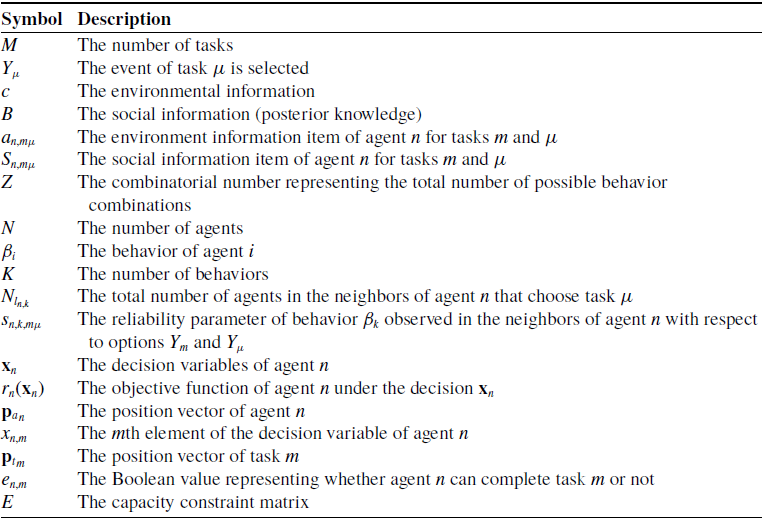
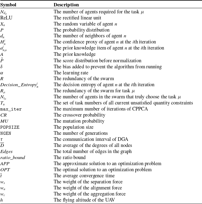
The paper is organized as follows: Section 2 provides the necessary preliminaries for the follow-up discussion. Section 3 then describes and rigorously proves the CPPC-GS in detail. Our method is experimentally verified and compared with other methods in Section 4. Section 5 concludes the paper with a summary of the main contents and contributions. A comprehensive summary of the key notations used throughout this paper is provided in the Nomenclature table located in the Appendix (Section A). Readers are encouraged to refer to it as needed.
2. Preliminaries
2.1. Bayesian estimation in fish schools
Perez-Escudero et al. [Reference Pérez-Escudero and de Polavieja15] developed a model including Bayesian estimation to explain the decision patterns of fish schools. First, each animal makes a Bayesian estimate of which behavior is most appropriate, taking into account environmental information and social information gathered by observing the behavior of other animals. Each animal then chooses a behavior based on the probabilities given by the Bayesian estimation.
In the original paper, let there be
 $M$
targets, denoted by
 ${Y_1},{Y_2}, \cdots ,{Y_M}$
, respectively. There are two types of information available to animals: environmental information and social information, denoted by
 $c$
and
 $B$
, respectively. Under the condition that the animal knows environmental information and social information, the probability that the agent
 $n$
chooses the target
 $Y_\mu$
can be expressed by Bayes theorem as follows:
 \begin{equation} P_n({Y_\mu }|c,B) = \frac {{P_n(B|{Y_\mu },c)P_n({Y_\mu }|c)}}{{\sum \nolimits _{m = 1}^M {P_n(B|{Y_m},c)P_n({Y_m}|c)} }} \end{equation}
Dividing both the numerator and denominator by the numerator, we obtain:
 \begin{equation} P_n({Y_\mu }|c,B) = \frac {1}{{\sum \nolimits _{m = 1}^M {{a_{n,m\mu }}{\text{ }}{S_{n,m\mu }}} }} \end{equation}
Where:
 \begin{equation} {a_{n,m\mu }} = \frac {{P_n({Y_m}|c)}}{{P_n({Y_\mu }|c)}} \end{equation}
 \begin{equation} \begin{aligned} S_{n,m\mu } &= \frac {P_n(B \mid Y_m, c)}{P_n(B \mid Y_\mu , c)} = \frac {Z \prod \limits _{i=1, i\neq n}^N P_n(\beta _i \mid Y_m, c)}{Z \prod \limits _{i=1, i\neq n}^N P_n(\beta _i \mid Y_\mu , c)} = \prod \limits _{k=1}^K \left ( \frac {P_n(\beta _k \mid Y_m, c)}{P_n(\beta _k \mid Y_\mu , c)} \right )^{N_{l_{n,k}}} = \prod \limits _{k=1}^K s_{n,k,m\mu }^{N_{l_{n,k}}} \end{aligned} \end{equation}
For the derivation of the equation, we assume that the behaviors
 $\beta$
in the social information
 ${B = \{ {\beta _1},{\beta _2}, \cdots ,{\beta _N}\}}$
referenced by an agent are mutually independent. Here,
 $Z$
is a combinatorial number representing the total number of possible behavior combinations;
 $N$
denotes the number of agents; and
 $K$
indicates the number of behavior categories after merging behaviors of the same type.
 ${N_l}_{_{n,\mu }}$
denotes the total number of agents in the neighbors of agent
 $n$
that choose task
 $\mu$
.
By derivation, the authors obtain:
 \begin{equation} P_n({Y_\mu }|c,B) = \bigg(\sum \limits _{m = 1}^M {{a_{n,m\mu }}} \prod \limits _{k = 1}^K {s_{n,k,m\mu }^{{{N_{l_{n,k}}}}}{\bigg)^{ - 1}}} \end{equation}
Here,
 ${s_{n,k,m\mu }} = {P_n}({\beta _k}|{Y_m},c)/{P_n}({\beta _k}|{Y_\mu },c)$
is the reliability parameter of behavior
 $\beta _k$
observed in the neighbors of agent
 $n$
with respect to options
 $Y_m$
and
 $Y_\mu$
. The term
 ${P_n}({\beta _k}|{Y_m},c)$
denotes the probability that an agent perceives behavior
 $\beta _k$
(i.e., other agents selecting task target
 $Y_\mu$
) in the social information, given the environmental information and the condition that agent
 $n$
selects task target
 $Y_m$
. There can be as many as
 $K(M-1)$
independent reliability parameters, though in practice, not all of them are necessarily independent.
 $a_{n,m\mu }$
is called the environmental information term and represents the ratio between the probabilities of selecting target
 $m$
and target
 $\mu$
given the environmental information
 $c$
.
 $s_{n,k,m\mu }$
is the social information item for agent
 $n$
. The article describes that under the influence of environmental information and social information, animals use Bayesian estimation and probability matching methods to make decisions through sequential patterns. This approach can well explain the collective decision-making behavior of animals.
A key inspiration for our probabilistic approach comes from the study of collective decision-making in animal groups, particularly the Bayesian estimation model observed in fish schools [Reference Pérez-Escudero and de Polavieja15]. In the original biological study, the authors tested the model using the collective behavior of three-spined sticklebacks (Gasterosteus aculeatus). The model posits that each individual fish continuously observes the choices of its neighbors and integrates this social information with its own private information about the environment using a Bayesian framework to make movement decisions.
This biological process offers a powerful analogy for distributed multi-agent systems. In our method, a fish observing the choices of other fish corresponds to communication and information sharing among neighboring agents. A fish deciding which area to move to based on these observations corresponds to an agent calculating a selection probability and then making a decision based on that probability.
By adopting this Bayesian estimation in the fish schools paradigm, we can effectively model and solve the distributed task allocation problem, where autonomous agents emulate this bio-inspired process of social information integration and probabilistic decision-making to achieve efficient collective outcomes.
2.2. Studied problem
Let
 $\mathbf{x}_n$
be defined as a one-hot vector of length
 $M$
, where the index of the element with a value of 1 corresponds to the index of the selected task. The cost from agent
 $n$
to the task represented by
 $\mathbf{x}_n$
is defined as the Euclidean distance between them, i.e.,
 \begin{equation} {r_n}(\mathbf{x}_n) = \left \| {{{\mathbf{p}}_{{a_n}}} - \sum \limits _{m = 1}^M {{x_{n,m}}} {{\mathbf{p}}_{{t_m}}}} \right \| \end{equation}
 ${\mathbf{p}}_{a_n}$
is the position vector of agent
 $n$
, and
 ${\mathbf{p}}_{t_m}$
is the position vector of task
 $m$
.
 $x_{n,m}$
is the
 $m$
th element of
 $\mathbf{x}_n$
. It should be noted that the cost function is defined in Eq. (6) represents a straightforward, widely utilized, and highly practical scenario in task allocation problems. In the existing literature, various cost metrics are established based on specific application contexts, including travel distance and energy consumption [Reference Yan and Xia32, Reference Wang, Li, Li, Cao and Wang33], execution time [Reference Su, Wang, Jia, Guo and Ding34], and profit [Reference Liu, Tan, Liang and Ding35]. Given that this study primarily focuses on the physical energy consumption and travel efficiency of agents moving toward allocated task points, the Euclidean distance is adopted as an intuitive proxy to quantify the cost of this static snapshot. Furthermore, the proposed algorithm framework exhibits strong modularity; hence, the distance-based cost can be readily substituted with other customized cost formulations depending on specific task requirements without affecting the underlying distributed coordination mechanism.
This work addresses a MR-TA problem where tasks are collaborative by nature, meaning that a single task can be executed by multiple agents simultaneously. This model inherently avoids the issue of assignment conflicts commonly found in exclusive allocation problems. For the distributed framework, we assume that the total number of agents,
 $N$
, is known to each agent upon completion of the system initialization phase. This task allocation is expressed as follows:
 \begin{equation} \begin{array}{*{20}{c}} {\min {\kern 1pt} \sum \limits _{n = 1}^N {r_n}(\mathbf{x}_n) } \\ {{\text{subject to}}\;\;\;{\kern 1pt} {\sum \limits _{m = 1}^M {{x_{n,m}} = 1}} ,{\text{ }}n = 1, \ldots ,N,{\text{ }}{x_{n,m}} \in \left \{ {0,1} \right \}} \\ {\sum \limits _{m = 1}^M {{e_{n,m}} \cdot {x_{n,m}} = 1} ,{\text{ }}n = 1, \ldots ,N,{\text{ }}{x_{n,m}} \in \left \{ {0,1} \right \}} \\ \sum \limits _{n = 1}^N {{x_{n,\mu }}} \geqslant {N_{{d_\mu }}},{\text{ }}\mu = 1, \ldots ,M \end{array} \end{equation}
Let
 $e_{n,m}$
be an element of the capacity constraint matrix
 $E$
, representing a Boolean value that indicates whether agent
 $n$
is capable of completing task
 $m$
or not.
 $N_{{d_\mu }}$
represents the number of agents required for the task
 $\mu$
.
The problem addressed in this paper is as follows. Under the premise that there is a lower bound on the number of agents required for each task and the tasks that agents can perform are limited, the sum of the distance costs of the agents to the task point is minimized through a distributed coordination mechanism where agents make decisions based on local information and limited communication with neighbors. And it can handle dynamic changes in task locations in real-time. As shown in Figure 1.
Studied problem.

Figure 1. Long description
A diagram of a multi-agent system. Panel A: The diagram shows three task areas labeled Task area 1, Task area 2, and Task area 3, each with a specific number of agents required. Agents are represented by different shapes: squares, triangles, and circles, each color-coded to match their respective task areas. The agents are interconnected by dashed lines, indicating the communication topology. A legend in the bottom left corner shows the capability constraints of the agents. Panel B: The diagram illustrates the deployment of redundant agents. Agents are grouped within their respective task areas, connected by dashed lines to show communication. The capability constraints legend is repeated to indicate the roles of the agents.
In Figure 1, circles with different colors represent different tasks. A brown edge between two agents indicates a communication link, which is established whenever their distance falls below a predefined threshold. The markers (circles, squares, and triangles) represent the agents, and their colors represent their decisions at that moment, corresponding to the color of the circle. The markers with different shapes have different capability constraints. The bottom left shows the agent-task capability constraints.
3. Confidence proxy-driven posterior correction and greedy swapping method (CPPC-GS)
3.1. Confidence proxy-driven posterior correction algorithm (CPPCA)
3.1.1. Method
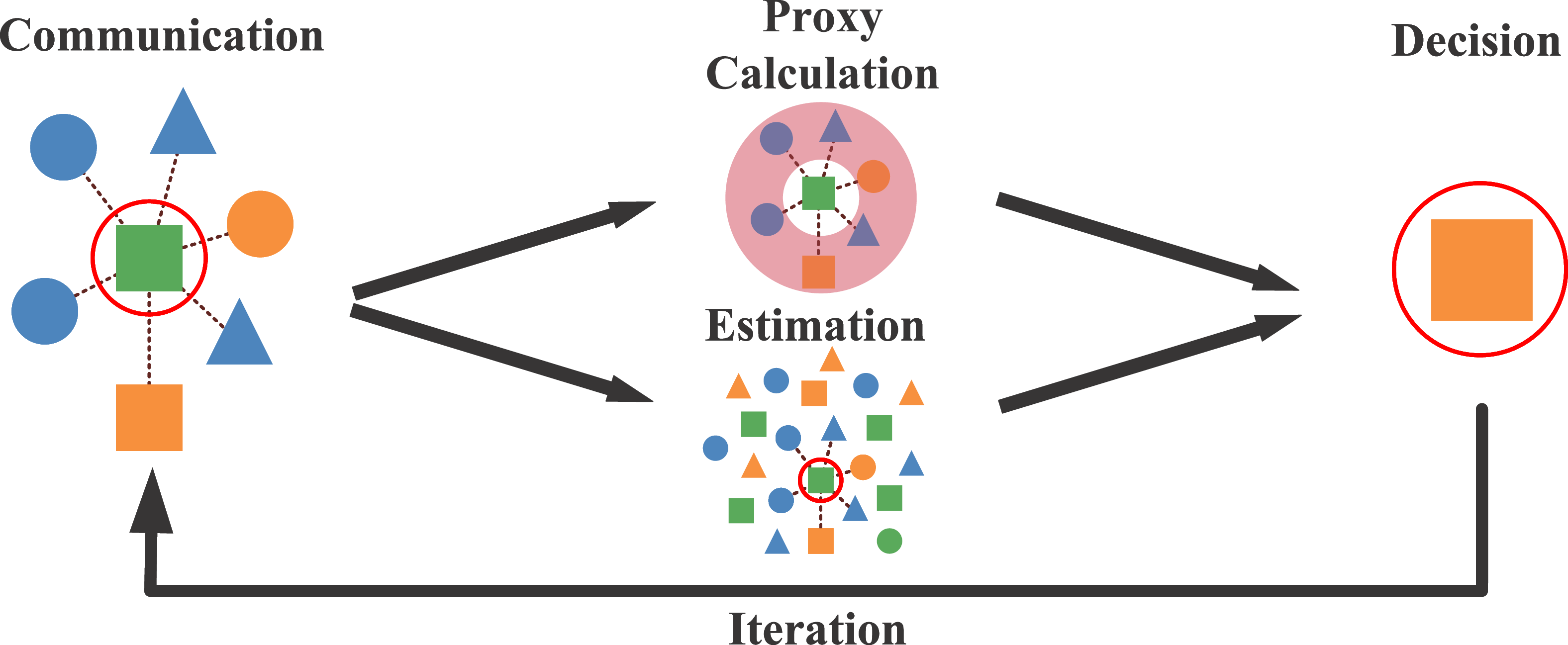
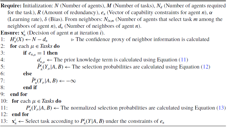
The algorithm is based on the idea of using neighbor information to estimate swarm information. By comprehensively considering the prior knowledge and neighbor information, the constraint is satisfied in several iterations. The architecture of the algorithm is shown in Figure 2.
Architecture of the CPPCA.

Inspired by the use of social and environmental information to regulate the selection probabilities, we propose CPPCA in this section. When this article refers to an agent’s neighbors, it includes the agent itself. The satisfaction constraint described in Section 2.1 governs the adjustment of the number of agents. Specifically, if the current number of agents assigned to a task is insufficient to meet the task requirements, more existing agents are reallocated (switched) to that task; if it is sufficient, the allocation is maintained without reduction. This logic of ”additive but non-subtractive” adjustment is functionally analogous to the behavior of a rectified linear unit (ReLU), as formulated in Eq. (8).
 \begin{equation} \operatorname {ReLU} \left ( x \right ) = \max\!(x,0) \end{equation}
Information entropy is a measure used to quantify the uncertainty of information in information theory. The higher the entropy, the greater the system’s uncertainty, and vice versa. The definition of information entropy is based on probability theory. If a random variable
 $X$
takes the possible values
 ${X_1},{X_2},{} \ldots ,{X_N}$
, and the corresponding probability distributions are
 $P({X_1}),{}P({X_2}),{} \ldots ,{}P({X_N})$
, the entropy
 $H(X)$
of this random variable is defined as follows:
 \begin{equation} H(X) = - \sum \limits _{n = 1}^{N} {P({X_n}){\text{log}}P({X_n})} \end{equation}
For distributed task allocation, the random variable
 $X$
should represent the set of task choices of all agents in the swarm. Where the choices of the neighbors of agent
 $n$
are known, the choices of the non-neighbors need to be estimated.
 $P({X_n})$
stands for the probability of
 $X_n$
, where the probability is estimated in frequency. In this way, the neighbor information entropy of agent
 $n$
represents the uncertainty of the information about its neighbors.
In this paper, we assume that the total number of tasks is
 $M$
, and the number of neighbors of agent
 $n$
is
 $d_n$
. In general, the number of elements in
 $X$
should be of magnitude close to
 $M^{N - \sum _{m = 1}^M{N_l}_{_{n,m}}}$
. Counting the frequencies of each
 $X_i$
is computationally expensive. Let’s assume that none of the
 $X_i$
are repeated, that is, they all have frequency 1; we also assume that the agent has no capacity constraints, so the probability of each choice is
 $1/{M^{N - {d_n}}}$
, and the number of elements in
 $X$
is
 $M^{N - {d_n}}$
. In Eq. (9), the logarithm is generally base 2, and the unit is bit. But you could take other log bases. For the sake of conciseness, let
 $M$
be the base, then the confidence proxy
 $H_n^i(X)$
of agent
 $n$
at the
 $i$
th iteration of the algorithm is approximately as follows:
 \begin{equation} \begin{aligned} H_n^i(X) &\approx - \sum _{i = 1}^{M^{N - d_n}} \frac {1}{M^{N - d_n}} \log _{M}\!\Bigl (\frac {1}{M^{N - d_n}}\Bigr ) = \log _{M}\!\bigl (M^{N - d_n}\bigr ) = N - d_n \end{aligned} \end{equation}
That is,
 $H_n^i(X)$
can be approximated by the number of non-neighbors of agent
 $n$
at iteration
 $i$
. This is a monotone heuristic proxy for neighborhood completeness. It makes intuitive sense because the more non-neighbors an agent has, the less reliable information it has and the less confidence it has. It is worth noting that this approximation does not influence the optimal solution of Eq. (7). The confidence proxy essentially determines the update magnitude of the algorithm. Although approximated, its relative scale preserves the correct reflection of the reliability of neighborhood information, thereby ensuring convergence to the theoretical optimum while significantly reducing computational complexity.
In literature [Reference Pérez-Escudero and de Polavieja15], the environmental information item
 ${a_{m\mu }} = P({Y_m}|c)/P({Y_\mu }|c)$
. Referring to this definition, the prior knowledge item for task allocation of redundant multi-agents is set as follows:
 \begin{equation} a_{n,\mu }^i = \left \{ \begin{array}{l} {N_{{d_\mu }}},i = 1 \\[4pt] P_n^{i - 1}({Y_\mu }|A,B),i \ne 1 \end{array} \right . \end{equation}
At the first iteration,
 $a_{n,\mu }^1$
is set to the number of agents required for task
 $\mu$
(environmental knowledge).
 $A$
and
 $B$
are prior and posterior knowledge, respectively. In order to avoid that animals making decisions first have more influence on the group than other animals when making sequential decisions in literature [Reference Pérez-Escudero and de Polavieja15], CPPCA uses parallel decision-making and sets
 $a_{n,\mu }^i$
in subsequent iterations as the selection probability of task
 $\mu$
in the previous iteration. This is to inherit the corrected probabilities from the previous iteration.
Then the probability that agent
 $n$
chooses a task at iteration
 $i$
can be written as follows:
 \begin{equation} \begin{aligned} \tilde {P}_n^i({Y_\mu }|A,B) &= \ln \left \{ {{{\left [ {{{\left ( {\frac {{H_n^i(X)}}{N} + \delta } \right )}^{\alpha \operatorname {ReLU} \left ( {\frac {{{N_{{d_\mu }}}}}{{N - R}} - \frac {{{N_{{l_{n,\mu }}}}}}{{{d_n}}}} \right )}}} \right ]}^{ - 1}} \times a_{n,\mu }^i} \right \} \\ &= - \alpha \operatorname {ReLU} \left ( {\frac {{{N_{{d_\mu }}}}}{{N - R}} - \frac {{{N_{{l_{n,\mu }}}}}}{{{d_n}}}} \right )\ln \left ( {\frac {{H_n^i(X)}}{N} + \delta } \right ) \\ &\quad + \ln \left ( {a_{n,\mu }^i} \right ) \end{aligned} \end{equation}
 \begin{equation} P_n^i({Y_\mu }|A,B) = \frac {{\exp \left [ {\tilde {P}_n^i({Y_\mu }|A,B)} \right ]}}{{\sum \limits _{m = 1}^M {\exp \left [ {\tilde {P}_n^i({Y_m}|A,B)} \right ]} }} \end{equation}
Here,
 $\tilde {P}$
represents the selection scores, and
 $P$
represents the selection probability.
 $B$
stands for posterior knowledge. And
 $A$
represents the environment knowledge required by the number of task agents in the first iteration. In the subsequent iterations,
 $A$
in addition contains the knowledge learned in the previous iterations, collectively referred to as prior knowledge.
 $\delta$
is a bias added to prevent undefined logs at zero if the agent’s neighbors are the entire swarm. It can be set to a small positive real number.
 $\alpha$
is the learning rate, which is a positive real number greater than 1.
 $R$
denotes the redundant number of the swarm, which can be computed by
 $N - \mathop \sum \nolimits _{m = 1}^M {N_{{d_m}}}$
.
 $d_n$
denotes the number of neighbors of agent
 $n$
. It is calculated as follows:
 $\sum _{m = 1}^M{N_l}_{_{n,m}}$
. Meanwhile, the term
 ${N_{{d_\mu }}}/\left ( {N - R} \right ) - {N_l}_{_{n,\mu }}/{d_n}$
computes the difference between the proportion of the selected task
 $\mu$
among the neighbors of agent
 $n$
and the proportion required by environmental knowledge. The agent will use this difference to correct its own choice probabilities for the corresponding task with
 $\alpha$
learning rate. However, when the number of agents in the neighborhood that select task
 $\mu$
has satisfied the environmental knowledge constraint, the scores of selecting it will not be increased. In Eq. (13), the softmax operation is performed on the score of selecting each task.
The information entropy of the selection probability of agent
 $n$
at iteration
 $i$
is defined as follows:
 \begin{equation} Decision\_Entropy_n^i = - \sum \limits _{m = 1}^{M} {P_n^i({Y_m}|A,B){\text{log}}P_n^i({Y_m}|A,B)} \end{equation}
The CPPCA algorithm uses
 $Decision\_Entropy$
as the stopping criterion, halting the agent’s iteration when the entropy falls below a threshold
 $\epsilon$
, with a maximum iteration count set as a safeguard.
According to the formula, the larger
 $\alpha$
is, the stronger the agent will revise according to the posterior knowledge. And the probabilities of all non-optimal choices for each agent will approach 0 faster, and the agent’s decision will be more firm. So a large learning rate will not only increase the speed of convergence but also reduce the amplitude after convergence. The pseudocode of CPPCA is shown in Algorithm 1. The computational complexity per iteration per agent of CPPCA is
 $O\left [ {\max \left ( {{d_n},M} \right )} \right ]$
, and the message complexity is
 $O\left ( {{d_n}} \right )$
.
CPPCA for the ith iteration of agent n

3.1.2. Proof of convergence
This section will focus on the convergence proof that CPPCA can make the task allocation satisfy the constraints.
Definition 1 [Redundancy
 $R_\mu$
of for task
 $\mu$
]. The redundancy
 $R_\mu$
assigned to task
 $\mu$
is the redundant number of agents dedicated to that task. Let
 $T_u$
denote the set of task numbers of all current unsatisfied quantity constraints. The sum of redundancies across
 $T_u$
equals the total redundant number
 $R$
, i.e.,
 \begin{equation} \sum \nolimits _{\mu \in {T_u}} {{R_\mu }} = R \end{equation}
This allocation of redundancies
 $R_\mu$
is a key parameter for the subsequent analysis.
 $R_\mu$
does not possess a strict physical meaning, nor does it require any manual intervention or uniform real-world distribution. Instead,
 $R_\mu$
is purely an auxiliary theoretical construct (or virtual variable) designed exclusively to facilitate the mathematical proof of convergence.
Lemma 3.1.
Let
 $N_{{t_\mu }}$
denote the number of agents in the swarm that truly choose the task
 $\mu$
. To make the number of neighbors for agent
 $n$
 ${d_n} \geqslant N \cdot {N_l}_{_{n,\mu }}/\left ( {{N_{{t_\mu }}} + {R_\mu }} \right ),{}\forall \mu \in {T_u}$
,
 $d_n$
satisfies at least
 ${d_n} \geqslant N \cdot \sum \nolimits _{\mu \in {T_u}} {{N_l}_{_{n,\mu }}} /\left ( {\sum \nolimits _{\mu \in {T_u}} {{N_{{t_\mu }}}} + R} \right )$
under a reasonable allocation of
 $R_\mu$
.
Proof.
For constant
 ${N_l}_{_{n,\mu }}$
and
 $N_{{t_\mu }}$
,
 $N \cdot {N_l}_{_{n,\mu }}/\left ( {{N_{{t_\mu }}} + {R_\mu }} \right )$
is smaller for larger
 $R_\mu$
. It is not hard to find that there should exist an allocation of
 $R$
such that for
 $\forall \mu \in {T_u}$
, all
 $N \cdot {N_l}_{_{n,\mu }}/\left ( {{N_{{t_\mu }}} + {R_\mu }} \right )$
are equal. And this equal value is a lower bound on
 $d_n$
.
Suppose the value we want to find that is equal is
 $Const$
, that is:
 \begin{equation} \frac {{{N_l}_{_{n,\mu }}}}{{{N_{{t_\mu }}} + {R_\mu }}} = Const,{\text{ }}\forall \mu \in {T_u} \end{equation}
Since
 $\sum \nolimits _{\mu \in {T_u}} {{R_\mu }} = R$
and
 ${R_\mu } = {N_l}_{_{n,\mu }}/Const - {N_{{t_\mu }}},{}\forall \mu \in {T_u}$
are deduced from the above equation, we can obtain:
 \begin{equation} \frac {{\sum \nolimits _{\mu \in {T_u}} {{N_l}_{_{n,\mu }}} }}{{Const}} - \sum \nolimits _{\mu \in {T_u}} {{N_{{t_\mu }}}} = R \end{equation}
So:
 \begin{equation} Const = \frac {{\sum \nolimits _{\mu \in {T_u}} {{N_l}_{_{n,\mu }}} }}{{\sum \nolimits _{\mu \in {T_u}} {{N_{{t_\mu }}} + R} }} \end{equation}
Under this reasonable allocation of
 $R$
,
 $d_n$
satisfies at least
 ${d_n} \geqslant N \cdot \sum \nolimits _{\mu \in {T_u}} {{N_l}_{_{n,\mu }}} /\left ( {\sum \nolimits _{\mu \in {T_u}} {{N_{{t_\mu }}}} + R} \right )$
.
Theorem 3.2.
When the number of neighbors
 $d_n$
of agent
 $n$
satisfies
 ${d_n} \geqslant N - R$
, the neighbor-estimated global ratios meet the condition
 $N \cdot {N_l}_{_{n,\mu }}/{d_n} \leqslant {N_{{t_\mu }}} + {R_\mu },{}\forall \mu \in {T_u}$
. This implies that the overestimation of task requirements by an agent will not exceed the redundancy allocated to it.
Proof.
Due to the existence of redundancy
 $R$
, the neighbor information can reflect the whole with a certain error, which can be described as follows:
 \begin{equation} {N_{{t_\mu }}} - {R_\mu } \leqslant N \cdot \frac {{{N_l}_{_{n,\mu }}}}{{{d_n}}} \leqslant {N_{{t_\mu }}} + {R_\mu },{\text{ }}\forall \mu \in {T_u} \end{equation}
The middle part of Eq. (19) represents the number of task
 $\mu$
selected by the agent in the whole, estimated by the neighbor information, and the left and right sides are the upper and lower bounds given after considering the redundancy. Our concern is that the number of estimates is so high that the agent does not properly adjust its selection score. So only focus on the right two parts of the inequality here. Collation can be obtained:
 \begin{equation} {d_n} \geqslant \frac {{N \cdot {N_l}_{_{n,\mu }}}}{{{N_{{t_\mu }}} + {R_\mu }}},{\text{ }}\forall \mu \in {T_u} \end{equation}
By Lemma 3.1 and Eq. (20),
 $d_n$
satisfies at least the following:
 \begin{equation} {d_n} \geqslant \frac {{N \cdot \sum \nolimits _{\mu \in {T_u}} {{N_l}_{_{n,\mu }}} }}{{\sum \nolimits _{\mu \in {T_u}} {{N_{{t_\mu }}}} + R}} \end{equation}
In the extreme case, all agents that choose unsatisfied tasks are neighbors of agent
 $n$
, and conversely, all neighbors of agent
 $n$
are those selecting unsatisfied tasks, in which case the right-hand side of Eq. (21) scales as follows:
 \begin{equation} \frac {{N \cdot \sum \nolimits _{\mu \in {T_u}} {{N_{{l_{n,\mu }}}}} }}{{\sum \nolimits _{\mu \in {T_u}} {{N_{{t_\mu }}}} + R}} \leqslant \frac {{N \cdot \sum \nolimits _{\mu \in {T_u}} {{N_{{l_{n,\mu }}}}} }}{{\sum \nolimits _{\mu \in {T_u}} {{N_{{l_{n,\mu }}}}} + R}} = \frac {N}{{1 + R/\sum \nolimits _{\mu \in {T_u}} {{N_{{l_{n,\mu }}}}} }} \leqslant \frac {N}{{1 + R/{d_n}}} \end{equation}
In this case, the right-hand side of Eq. (21) is the largest, which is
 $N/\left ( {1 + R/{d_n}} \right )$
. Then the inequality relation of
 $d_n$
is as follows:
 \begin{equation} {d_n} \geqslant \frac {{N \cdot {d_n}}}{{{d_n} + R}} \end{equation}
Rearranging gives:
 \begin{equation} {d_n} \geqslant N - R \end{equation}
When
 ${d_n} \geqslant N - R$
, the error of the neighbor information is within the range that the redundancy can be filled.
Theorem 3.3.
If the number of neighbors of agent
 $n$
 $d_n$
is greater than
 $N - R$
, when the
 ${N_l}_{_{n,\mu }}/{d_n} \lt {N_{{d_\mu }}}/\left ( {N - R} \right )$
, that is, when the proportion of agents that select task
 $\mu$
in the overall information reflected by neighbor information does not satisfy the constraint, CPPCA can increase the selection scores of agent
 $n$
for task
 $\mu$
; conversely, CPPCA keeps the selection scores constant.
Proof.
When
 $i \gt 1$
, the formula can also be written as follows:
 \begin{equation} \begin{aligned} \tilde {P}_n^i({Y_\mu }|A,B) &= - \alpha \operatorname {ReLU} \left ( {\frac {{{N_{{d_\mu }}}}}{{N - R}} - \frac {{{N_{{l_{n,\mu }}}}}}{{{d_n}}}} \right )\ln \left ( {\frac {{H_n^i(X)}}{N} + \delta } \right ) + \ln \left ( P_n^{i - 1}({Y_\mu }|A,B) \right ) \end{aligned} \end{equation}
 $\mu$
is the task that the agent can choose within the capability constraint. When the
 ${N_l}_{_{n,\mu }}/{d_n} \lt {N_{{d_\mu }}}/\left ( {N - R} \right )$
, that is, when the proportion of agents that select task
 $\mu$
in the overall information reflected by neighbor information does not satisfy the constraint, Eq. (25) is transformed into:
 \begin{equation} \tilde {P}_n^i({Y_\mu }|A,B) = - \alpha \left ( {\frac {{{N_{{d_\mu }}}}}{{N - R}} - \frac {{{N_{{l_{n,\mu }}}}}}{{{d_n}}}} \right )\ln \left ( {\frac {{N-d_n}}{N} + \delta } \right ) + \ln \left ( P_n^{i - 1}({Y_\mu }|A,B) \right ) \end{equation}
Since
 $\delta$
is small and can be ignored,
 $\left [ {\left ( {N - {d_n}} \right )/N + \delta } \right ] \in (0,1)$
and
 $\left [ {{N_{{d_\mu }}}/\left ( {N - R} \right ) - {N_l}_{_{n,\mu }}/{d_n}} \right ] \in ( 0,1]$
,
 $\alpha \cdot \left [ {{N_{{d_\mu }}}/\left ( {N - R} \right ) - {N_l}_{_{n,\mu }}/{d_n}} \right ] \in (0 ,\alpha ]$
. When
 $\alpha \gt 1$
, the first term of Eq. (26) is greater than 0.
It follows from Theorem3.2 that the neighbor information can correctly reflect the overall information. The above derivation shows that the algorithm can always increase the selection score corresponding to a task when the number of agents choosing a task does not satisfy the constraint. Similarly, if the number of agents choosing a task satisfies the constraint, the algorithm can always keep the selection score corresponding to this task unchanged (due to the existence of the ReLU function).
Intuitively, the condition that the number of neighbors must exceed a certain threshold for CPPCA to converge is deeply tied to its estimation mechanism. The core philosophy of CPPCA relies on agents estimating the global task distribution of the population through the local task selections of their neighbors, followed by iterative strategy adjustments. This process fundamentally depends on estimation accuracy. When the number of neighbors is too small, the local observation acts as an unrepresentative sample, leading to poor estimation accuracy of the global state. Such unreliable estimations can easily mislead an agent’s decision-making process, causing its choice to deviate from the correct convergence direction. Therefore, a sufficiently large number of neighbors is required to guarantee the statistical reliability of the estimation, thereby ensuring the stable convergence of the algorithm.
However, due to the subsequent softmax operation on the selection probabilities, the increase in the selection score described in Theorem3.3 does not guarantee that the normalized selection probability will also increase. When another task has a larger demand for the number of agents than task
 $\mu$
, the selection probability of task
 $\mu$
may become smaller after normalization. But this is a better outcome for the swarm, as the agent will tend to choose tasks that require it more.
With the development of communication and iteration, the algorithm will continuously increase the selection probabilities of tasks whose constraints are not satisfied until the constraints are satisfied and the algorithm converges.
Theorem3.2 gives a lower bound on
 $d_n$
in a very extreme case, where it is practically impossible to encounter an iteration in which only the task with the smallest demand is satisfied. So in practice, the lower bound of
 $d_n$
is affected by the capacity constraint matrix
 $E$
and the initialization way, but it must be lower than
 $N-R$
.
3.2. Greedy swapping algorithm (GSA)
3.2.1. Method
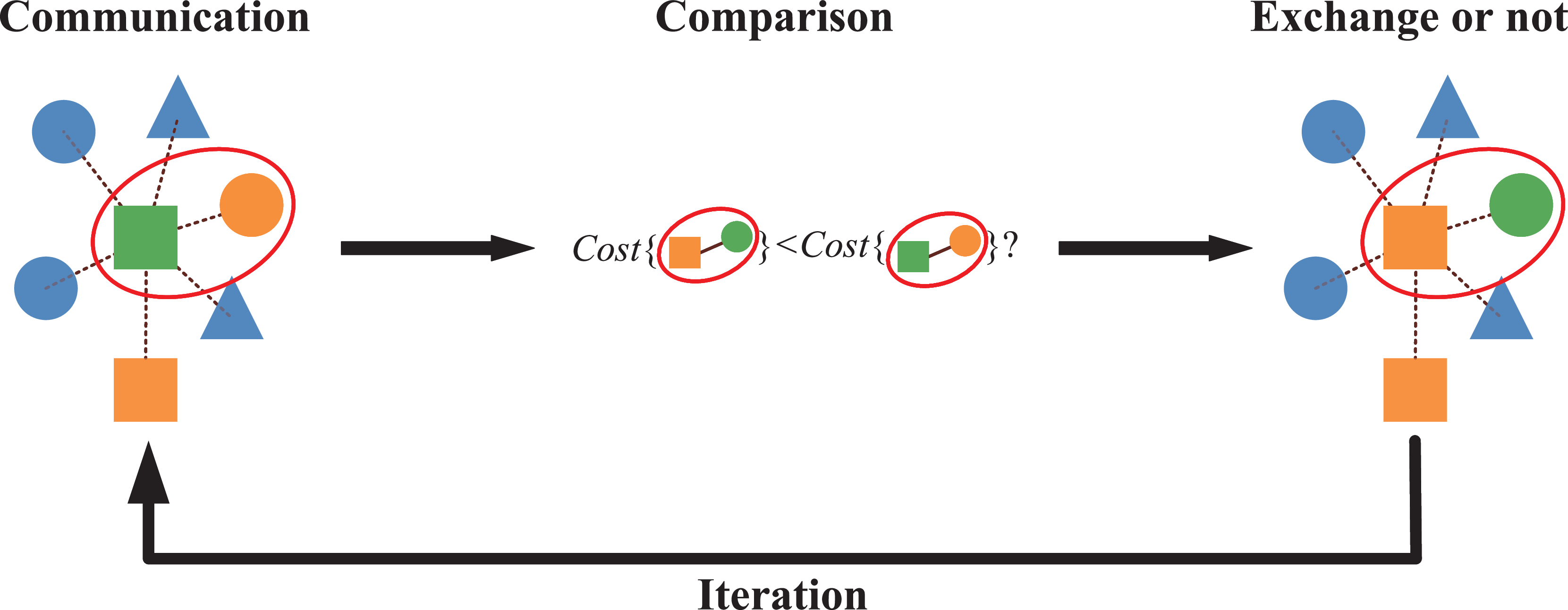
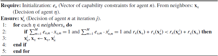
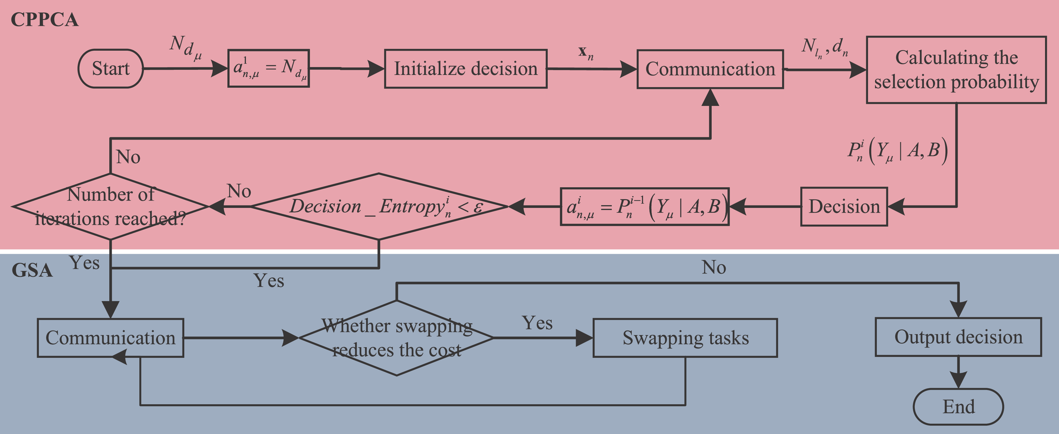
After the above decision process is completed, only one of the solutions satisfying the constraints is obtained. However, it is not the solution that minimizes the objective function. In this section, we will use GSA to solve this problem. For each agent, evaluate whether swapping tasks with all of its neighbors results in a decrease in the objective function. Note that this step requires both agents to complete the swapped task. If a swap is found that reduces the overall cost, the swap is implemented. This is repeated for all agents until no swap can further reduce the overall cost. The algorithm architecture is shown in Figure 3, and the detailed steps are summarized as Algorithm 2. The computational complexity per iteration per agent of GSA is
 $O\left ( {{d_n}} \right )$
, and the message complexity is
 $O\left ( {{d_n}} \right )$
.
Because the algorithm only performs swapping task operations, the satisfied quantity constraints are not changed. The GSA selects the current best decision at each step, but this can lead to a globally suboptimal solution, especially in complex multi-agent environments.
Architecture of the GSA.

GSA for the jth iteration of agent n

3.2.2. Proof of convergence
The convergence of the GSA can be analyzed under an asynchronous execution model. We model the process as one where each agent activates according to its own clock, attempting to negotiate task swaps with its neighbors. Convergence is guaranteed provided two key conditions hold: (1) the communication channels are eventually reliable (messages are not lost or delayed indefinitely), and (2) each agent is activated infinitely often. This ensures that the system can explore all possible swap pairs over time.
To handle transient conflicts that may arise from concurrency (e.g., two agents simultaneously attempting to swap with a common third agent), we assume a simple priority-based conflict resolution mechanism. In this scheme, each agent or task is assigned a unique priority. When conflicting swap proposals are detected, the proposal involving the higher-priority entity is executed. This deterministic resolution strategy ensures progress and does not affect the core argument for convergence, which relies on the monotonic improvement of the global objective function with each successful, non-conflicting swap.
The correctness and convergence of GSA will be illustrated from the following aspects.
Theorem 3.4.
Each swap of GSA makes the total cost
 $\sum \nolimits _{n = 1}^N {r_n}(\mathbf{x}_n^{\,j})$
decrease, and the algorithm will eventually converge to a local optimal state.
Proof.
Since the algorithm will only be possible to swap tasks if
 ${r_n}(\mathbf{x}_\eta ){\text{ + }}{r_\eta }(\mathbf{x}_n^{\,j})\lt {r_n}(\mathbf{x}_n^{\,j}){\text{ + }}{r_\eta }(\mathbf{x}_\eta )$
, let the total cost after swapping be
 $\sum \nolimits _{n = 1}^N {r_n}^\prime (\mathbf{x}_n^{\,j})$
,
 $\sum \nolimits _{n = 1}^N {r_n}^\prime (\mathbf{x}_n^{\,j}) \lt \sum \nolimits _{n = 1}^N {r_n}(\mathbf{x}_n^{\,j})$
. So the algorithm will eventually converge to a local optimal solution.
Theorem 3.5. If the total cost of GSA after each swap is strictly decreasing and a lower bound on the total cost exists, then the algorithm converges in finite steps.
Proof.
It follows from Theorem3.4 that the total cost of GSA after each swap strictly decreases. In addition, from a global perspective, there must be an optimal task allocation that satisfies the capability constraint
 $E$
of all agents. That is, there exists a lower bound on the total cost, so the algorithm converges to a near-optimal solution within a finite number of steps.
By Theorem3.4, the total cost strictly decreases after each swap. Therefore, the algorithm never revisits the same total cost value.
Crucially, since the number of agents and tasks is finite, the set of all possible task allocations is finite. Consequently, the set of possible total cost values that the algorithm can generate is also a finite set.
The algorithm produces a sequence of strictly decreasing total costs drawn from this finite set. It cannot generate an infinite sequence of distinct values, as that would require an infinite set of possible costs. Therefore, the algorithm must terminate after a finite number of swaps when no further strict improvement (i.e., cost reduction) is possible. Upon termination, the solution is a local optimum (or near-optimal solution) as guaranteed by the swap acceptance criterion.
In the worst case, the ratio bound of GSA is related to the number of agents and the communication topology, but the specific ratio bound can be determined empirically and experimentally.
3.3. Flow of the CPPC-GS
CPPC-GS mainly contains two parts: CPPCA and GSA. Firstly, CPPCA is used to make each individual learn the decision that needs to be made at the moment through the interaction with its neighbors, and then the decisions of the swarm meet the constraints. Then, under the premise that the constraints have been satisfied, the agent uses GSA to swap with its neighbors to reduce the cost of the swarm, thus solving the DCOP. This is shown in Figure 4.
The flow chart of the CPPC-GS.

4. Simulation results
4.1. Comparison between CPPC-GS and others in the case of connected graph
4.1.1. Parameter settings
To ensure a fair and reproducible comparison, the following protocol was adhered to for all experiments reported in this section. All algorithms were evaluated using the same number of tasks (
 $M$
), the same number of agents (
 $N$
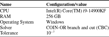
), identical agent-task capability matrices, and the same random seeds for generating communication graph topologies. The hardware configuration and solver setup are shown in Table I. For calculating the ratio bound, the centralized optimal solution was obtained by solving the ILP problem defined in Eq. (7) using the COIN-OR branch and cut (CBC) solver. No time limit was imposed to ensure the global optimum was found.
Hardware configuration and solver setup.

Table I. Long description
A table with two columns and five rows. The columns are labeled ‘Name’ and ‘Configuration/value’. The rows are as follows: Row 1: Name, CPU; Configuration/value, Intel(R) Core(TM) i9-14900KF. Row 2: Name, RAM; Configuration/value, 256 GB. Row 3: Name, Operating System; Configuration/value, Windows. Row 4: Name, Solver; Configuration/value, COIN-OR branch and cut (CBC). Row 5: Name, Tolerance; Configuration/value, 10^-7.
The Consensus-Based Auction Algorithm (CBAA) can solve the distributed single task allocation and can obtain the approximate optimal solution in finite time under the premise that the communication topology is not a complete graph [Reference Choi, Brunet and How9]. In the allocation process, the agent does not need to know the total payoff of the group, but it requires the communication topology graph to be connected at any time; otherwise, there will be conflicts.
The consensus link of CBAA can resolve the conflict of swarm task selection. Therefore, even if the number of agents is equal to the required number of tasks, the tasks can still be assigned accurately to meet the required number of tasks and minimize the cost function. The task allocation in this paper can be viewed as an
 $M\lt N$
allocation. That is, the number of tasks is smaller than the number of agents, and each task can be repeatedly selected by the agent. Based on this, we can multiply the tasks by the number of agents required, such that
 $M=N$
after augmentation. The payoff is defined as the inverse of Euclidean distance if the agent can complete a task and zero if the agent cannot. This single allocation problem is then solved using CBAA. This method inherits the desirable convergence properties of CBAA. Its performance is optimal when the cloned tasks are truly independent and interchangeable, which is a valid assumption in our target application.
A genetic algorithm (GA) is an optimization algorithm that simulates natural selection and genetic mechanisms (such as crossover and mutation). It searches for the global optimal solution through iterative evolution of the population, which is widely used in combinatorial optimization, machine learning, and other fields. In this paper, GA, a representative centralized optimization method, is selected to compare with CPPC-GA.
Decentralized genetic algorithm (DGA) parallelizes genetic algorithms across a team of agents [Reference Patel, Rudnick-Cohen, Azarm, Otte, Xu and Herrmann36]. Each agent periodically shares its current best solution with the other agents and incorporates any solutions it receives into its population.
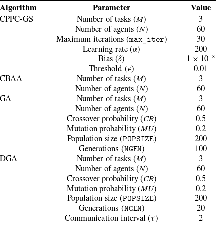
The simulation parameters selected for a swarm size of 60 are listed in Table II. The range of the
 $\alpha$
is related to the scale of the update amount. The recommended range for the
 $\alpha$
is 10 to
 $10^4$
, based on the scale of the parameters for common task allocation problems.
Simulation parameters.

Table II. Long description
The table compares simulation parameters for four algorithms: CPPC-GS, CBAA, GA, and DGA. It has four columns: Algorithm, Parameter, and Value. The table lists the values for each parameter across the different algorithms. Row 1: Algorithm, CPPC-GS. Row 2: Parameter, Number of tasks (M). Row 3: Value, 3. Row 4: Parameter, Number of agents (N). Row 5: Value, 60. Row 6: Parameter, Maximum iterations (max_iter). Row 7: Value, 30. Row 8: Parameter, Learning rate (alpha). Row 9: Value, 200. Row 10: Parameter, Bias (delta). Row 11: Value, 1 times 10 to the power of -8. Row 12: Parameter, Threshold (epsilon). Row 13: Value, 0.01. Row 14: Algorithm, CBAA. Row 15: Parameter, Number of tasks (M). Row 16: Value, 3. Row 17: Parameter, Number of agents (N). Row 18: Value, 60. Row 19: Algorithm, GA. Row 20: Parameter, Number of tasks (M). Row 21: Value, 3. Row 22: Parameter, Number of agents (N). Row 23: Value, 60. Row 24: Parameter, Crossover probability (CR). Row 25: Value, 0.5. Row 26: Parameter, Mutation probability (MU). Row 27: Value, 0.2. Row 28: Parameter, Population size (POPSIZE). Row 29: Value, 200. Row 30: Parameter, Generations (NGEN). Row 31: Value, 100. Row 32: Algorithm, DGA. Row 33: Parameter, Number of tasks (M). Row 34: Value, 3. Row 35: Parameter, Number of agents (N). Row 36: Value, 60. Row 37: Parameter, Crossover probability (CR). Row 38: Value, 0.5. Row 39: Parameter, Mutation probability (MU). Row 40: Value, 0.2. Row 41: Parameter, Population size (POPSIZE). Row 42: Value, 200. Row 43: Parameter, Generations (NGEN). Row 44: Value, 20. Row 45: Parameter, Communication interval (tau). Row 46: Value, 2.
The average degree is the average of the degrees of all nodes, which can be calculated by the following formula:
 \begin{equation} \overline D = \frac {{2Edges}}{N} \end{equation}
where
 $Edges$
is the total number of edges in the graph and
 $N$
is the total number of nodes in the graph. This parameter can reflect the connectivity of a connected graph. Since the convergence time of CPPC-GS, CBAA, and DGA is affected by the number of neighbors of each node, it should be consistent in the subsequent comparison, which is taken as 20 here. The graphs in this section are randomly generated at this average degree.
4.1.2. Feasibility and advantages of CPPC-GS
Using the simulation parameters defined above, when the communication topology is a connected graph, CPPC-GS is used for redundant agent task allocation. The simulation results of CPPCA are shown in Figure 5.
The curve of quantity change.

The ordinate represents the number of agents that selected task
 $\mu$
. The abscissa represents the number of iterations. The broken lines with different colors indicate that the number of agents selecting task
 $\mu$
varies with the number of iterations. The dashed line is the constraint of the environment information. Under the premise of agent redundancy, CPPCA can satisfy the constraint of environment information within the maximum number of iterations, which is also the criterion to judge the convergence of CPPCA.
Figure 6 shows the change curve of the information entropies of the selection probabilities of the agents during the iterations.
Change in the information entropies of the selection probabilities.

Figure 6. Long description
The image contains a grid of 50 line graphs, each representing changes in information entropies of selection probabilities. Each graph has a horizontal axis labeled from 0 to 30 and a vertical axis labeled from 0 to 1. The legend indicates that the blue line represents the entropy of p. The graphs show various patterns of entropy changes, including sharp drops, gradual declines, fluctuations, and steady states. Each graph illustrates different behaviors of the selection probabilities under varying conditions, highlighting the diversity in entropy changes across different scenarios.
The reduction in information entropies reflects the reduction in selection uncertainty. After multiple iterations, the information entropies of selection probabilities of most agents converged to 0 or some other value, indicating that these agents had understood the task they should choose or the probability they should assign. The information entropies of a small number of agents do not converge, which is because they have relatively few neighbors, but this does not affect the convergence of the swarm.
CPPCA can regulate the selection probability by the prior term and the posterior term in the formula. When the agent’s ability to complete a task is weak, its own selection probability is strongly corrected by the decisions of its neighbors so that the swarm’s decisions will converge after a finite number of iterations.
Next, we reduce the total cost by swapping tasks with GSA. The resulting curve of the total cost as a function of swap is shown in Figure 7.
The curve of the cost change.

Ratio bound is a common index to measure the goodness of an approximate solution, which is defined by the following formula:
 \begin{equation} ratio\_bound = \max \!\left\{ \frac {{APP}}{{OPT}},\frac {{OPT}}{{APP}}\right\} \end{equation}
where
 $APP$
is an approximate solution to an optimization problem and
 $OPT$
is the optimal solution to this problem. So the bigger
 $ratio\_bound$
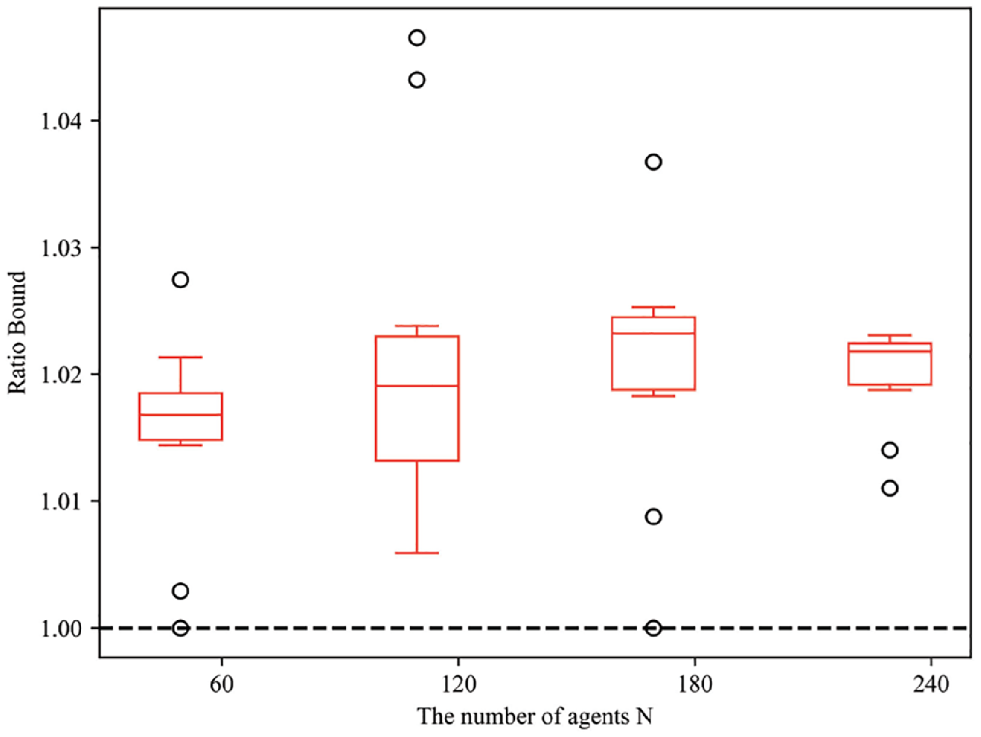
is, the worse the solution is. After repeated experiments, ILP is used as the exact benchmark method to generate the optimal solution. The simulation under different problem sizes is carried out, and the ratio bound obtained is shown in Figure 8.
Box plot of ratio bound as a function of problem size.

The figure shows that the approximate solution produced by GSA in CPPC-GS is within about 2% of the optimal solution and is independent of the problem size. The convergence time comparison of the four algorithms is shown in Figure 9.
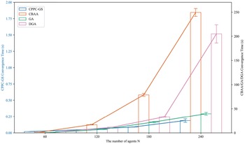
Comparison of convergence time.

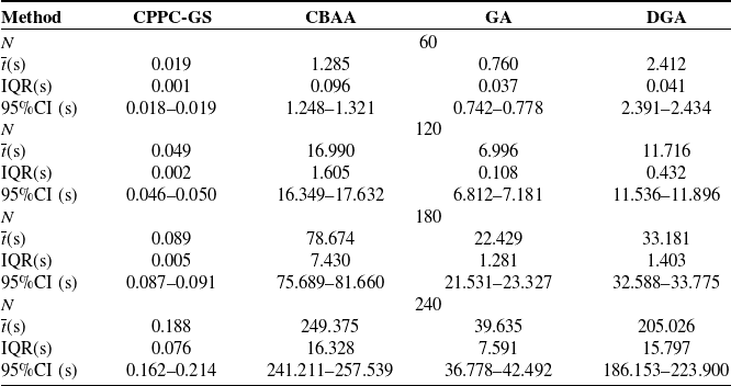
The different algorithms in Figure 9 have their own independent Y-axis. After a finite number of iterations, four methods can meet the constraints, and the stabilities of the algorithms are all good after repeated running. Without sacrificing optimality, CPPC-GS is more efficient than other algorithms, which take a long time to reach consensus, while GA and DGA randomly approach the optimal solution. With the increase of the number of agents, the dimension explosion of CBAA, GA, and DGA occurs, and their convergence time rises rapidly. However, the convergence time of CPPC-GS increases almost linearly. When the number of agents reaches 240, the average runtime of CBAA, GA, and DGA no longer meets the real-time requirement. It is foreseeable that when solving large-scale problems, the advantages of applying CPPC-GS to solve such problems will further increase. In the simulation, we also found that when using CBAA to solve the task allocation in this paper, there will be a situation where the corresponding capacity constraint is 0 but the task is still assigned. Due to the algorithmic logic of CBAA, there will be cases where the bids on the tasks with a capacity constraint of 1 are smaller than those of other agents, and they will have to choose the task with a capacity constraint of 0. Limited by CPU cores in PC-based multi-process simulation, multiple agents share one process. Intra-process serial overhead combined with decentralized coordination costs (e.g., inter-process communication) restricts efficiency, making DGA’s runtime no better than the centralized GA in this study.
A summary table of the performance comparison is shown in Table III.
To validate the statistical significance of these performance improvements, we conducted the Wilcoxon signed-rank test between CPPC-GS and each comparative method. The results show that all p-values from the tests are less than 0.05, demonstrating that the performance advantages of CPPC-GS over CBAA, GA, and DGA are statistically significant at the 95% confidence level.
Performance comparison.

Table III. Long description
The table compares the performance of four methods: CPPC-GS, CBAA, GA, and DGA across different sample sizes (N) and metrics including mean (s), interquartile range (IQR), and 95% confidence interval (CI). The table has 5 rows and 8 columns. Column headers are Method, CPPC-GS, CBAA, GA, and DGA. Row labels include N, mean (s), IQR(s), and 95%CI (s) for each sample size (60, 120, 180, 240). Row 1: Method, CPPC-GS, CBAA, GA, DGA. Row 2: N, , , 60, . Row 3: mean (s), 0.019, 1.285, 0.760, 2.412. Row 4: IQR(s), 0.001, 0.096, 0.037, 0.041. Row 5: 95%CI (s), 0.018-0.019, 1.248-1.321, 0.742-0.778, 2.391-2.434. Row 6: N, , , 120, . Row 7: mean (s), 0.049, 16.990, 6.996, 11.716. Row 8: IQR(s), 0.002, 1.605, 0.108, 0.432. Row 9: 95%CI (s), 0.046-0.050, 16.349-17.632, 6.812-7.181, 11.536-11.896. Row 10: N, , , 180, . Row 11: mean (s), 0.089, 78.674, 22.429, 33.181. Row 12: IQR(s), 0.005, 7.430, 1.281, 1.403. Row 13: 95%CI (s), 0.087-0.091, 75.689-81.660, 21.531-23.327, 32.588-33.775. Row 14: N, , , 240, . Row 15: mean (s), 0.188, 249.375, 39.635, 205.026. Row 16: IQR(s), 0.076, 16.328, 7.591, 15.797. Row 17: 95%CI (s), 0.162-0.214, 241.211-257.539, 36.778-42.492, 186.153-223.900.
 $^{1}$
 $\overline {t}$
: average convergence time (seconds)
 $^{2}$
IQR: interquartile range of average convergence time (seconds)
 $^{3}$
95%CI: confidence interval of average convergence time (seconds).
4.1.3. Scalability evaluation
To investigate the impact of neighbor degree on the convergence of CPPC-GS, we conducted tests on the algorithm with different neighbor degree values under the premise that
 $N$
is set to 60, and the results are illustrated in the Figure 10.
Convergence vs. neighbor degree.

As can be observed from the figure, when the neighbor degree is set to 5 or 10, each agent obtains limited posterior knowledge and faces high uncertainty in group decision estimation. Consequently, the resulting estimation error cannot be compensated for by the corresponding redundancy, leading to the failure of CPPC-GS to converge.
To investigate the impact of redundancy on the convergence of CPPC-GS, we conducted tests on the algorithm with different redundancy levels, and the results are illustrated in the Figure 11.
Convergence vs. redundancy.

As can be observed from the figure, when the redundancy is set to 0, 5, or 10, the estimation error of each agent cannot be compensated for by the corresponding redundancy. Consequently, CPPC-GS fails to converge.
4.2. CPPCA in the case of a non-connected graph
Using the parameters defined in Table II, when the communication topology is a non-connected graph, the general auction algorithm cannot completely resolve the conflict through neighbor information, so the final result cannot meet the constraints. However, CPPCA uses neighbor information to approximate the overall selection. When the graph is not connected, CPPCA still uses the choice of neighbors to estimate the overall choice and then makes the choice of swarm satisfy the constraint, as shown in Figure 12.
CPPCA when the graph is not connected.

Figure 12. Long description
Panel A: A scatter plot depicts the communication network topology. The x-axis is labeled X/m and ranges from -6 to 6. The y-axis is labeled Y/m and ranges from -6 to 6. The plot shows various nodes connected by lines, with different symbols representing different types of nodes. Panel B: A line graph shows the curve of quantity change in CPPCA. The x-axis is labeled Iteration and ranges from 1 to 30. The y-axis is labeled Number of agents and ranges from 10 to 35. The graph includes three lines representing Task 1, Task 2, and Task 3, each with different colors. The lines show the number of agents assigned to each task over iterations, with visible fluctuations and trends.
As shown in Figure 12a, the communication topology is completely two isolated subislands, which belongs to the case of a non-connected graph. Due to the advantage of estimation, CPPCA’s convergence is only related to the average degree of the graph, independent of whether it is connected or not. After a few iterations, the numbers of agents selected for all three tasks satisfy the constraints in a component-wise manner.
4.3. Dynamic performances of CPPC-GS and CBAA
4.3.1. Parameter settings
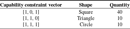
In the simulation of this section, according to the capability constraint matrix, the agents in the swarm can be divided into three categories, which are represented by squares, circles, and triangles, respectively. The capability constraints and number of agents are defined in Table IV.
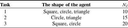
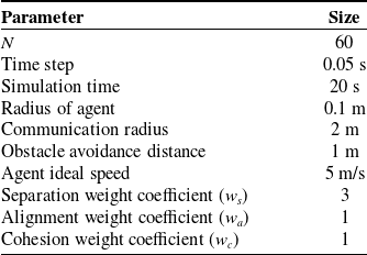
Since each task can only be selected by a subset of agents, the shapes of agents that should appear in different task points in the simulation results are shown in Table V. According to Table IV, the square agent can complete tasks 1 and 3, so the square agent can appear within task points 1 and 3. On the contrary, if an agent inconsistent with Table V appears in the task point, it means that the result of task allocation does not comply with the capability constraint. The motion of the swarm uses the Reynolds-Boid model, and the parameters used are defined in Table VI.
The low-level flocking behavior of the agent swarm is governed by a motion control model based on the boids framework. Separation (governed by weight
 $w_s$
) compels an agent to steer away from its local flock mates to avoid crowding. Alignment (governed by weight
 $w_a$
) steers an agent towards the average heading of its local neighbors. Cohesion (governed by weight
 $w_c$
), in contrast, directs an agent to move towards the average position of its local flock mates. The weights
 $w_s$
,
 $w_a$
, and
 $w_c$
tune the relative influence of these three competing forces.
The positions of tasks 2 and 3 are constant and are (0,8) and (5,8), respectively. The location of task 1 is time-varying. Its trajectory is defined as a circle with center (0,0) and radius 5 m. The motion speed is
 $1\pi$
m/s. Task 2 will become inaccessible for 6s–14s and appear for the rest of the time.
Different types of agents.

Table IV. Long description
Table with three rows and three columns. The first column lists capability constraint vectors as [1,"0", 1], [1,"1", 0], and [1,"1", 1]. The second column lists shapes as Square, Triangle, and Circle. The third column lists quantities as 40, 10, and 10 respectively.", "EDH": "Table categorizing agents by shape and quantity.
The shapes of the agents that should appear in the task point.

Table V. Long description
A table with three rows and three columns. The columns are labeled Task, The shape of the agent, and N subscript a. The rows are as follows: Row 1: Task 1, Square, circle, triangle, N subscript a 10. Row 2: Task 2, Circle, triangle, N subscript a 15. Row 3: Task 3, Square, circle, N subscript a 20.
Dynamic task allocation corresponding parameters.

Table VI. Long description
A table with two columns labeled Parameter and Size. The table contains six rows with the following data: Row 1: Parameter, N; Size, 60. Row 2: Parameter, Time step; Size, 0.05 s. Row 3: Parameter, Simulation time; Size, 20 s. Row 4: Parameter, Radius of agent; Size, 0.1 m. Row 5: Parameter, Communication radius; Size, 2 m. Row 6: Parameter, Obstacle avoidance distance; Size, 1 m. Row 7: Parameter, Agent ideal speed; Size, 5 m/s. Row 8: Parameter, Separation weight coefficient (w s); Size, 3. Row 9: Parameter, Alignment weight coefficient (w a); Size, 1. Row 10: Parameter, Cohesion weight coefficient (w c); Size, 1.
4.3.2. The real-time performance and emergence
The CPPC-GS and CBAA are designed to solve a static instance of the task allocation problem. To evaluate their performance in dynamic environments, we adopt a receding-horizon approach. Specifically, at each discrete time step, the current state of the system (agent positions and the set of available tasks) is treated as a static snapshot. The CPPC-GS and CBAA are then invoked to compute an allocation for this snapshot. This process repeats at every time step, allowing the system to adapt to new tasks and agent state changes.
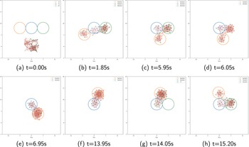
The dynamic task allocation simulations of CPPC-GS and CBAA are shown in Figures 13 and 14, respectively. In the figures, the top right legend shows how many more agents are needed for each task.
Simulation of dynamic task allocation for CPPC-GS.

Figure 13. Long description
Panel A: At time 0.00 seconds, three circles are shown with no data points inside them. The circles are labeled as Unsatisfied. Panel B: At time 1.85 seconds, data points start appearing within the circles, with some points overlapping between circles. The circles are labeled as Unsatisfied. Panel C: At time 5.95 seconds, more data points are within the circles, with increased overlap. The circles are labeled as Unsatisfied. Panel D: At time 6.05 seconds, data points continue to cluster within and overlap the circles. The circles are labeled as Unsatisfied. Panel E: At time 6.95 seconds, data points are densely packed within the circles, with significant overlap. The circles are labeled as Unsatisfied. Panel F: At time 13.95 seconds, data points are densely packed within the circles, with significant overlap. The circles are labeled as Unsatisfied. Panel G: At time 14.05 seconds, data points are densely packed within the circles, with significant overlap. The circles are labeled as Unsatisfied. Panel H: At time 15.20 seconds, data points are densely packed within the circles, with significant overlap. The circles are labeled as Unsatisfied.
Simulation of dynamic task allocation for CBAA.

After the simulation starts, the swarm continuously makes decisions based on the distance from the task point and its own capabilities constraints, as shown in Figures 13a and 14a, and then moves towards the assigned task point. Note that CPPC-GS and CBAA are called repeatedly throughout the simulation to update the agents’ decisions. Task 1 is motion, and the agent can achieve tracking according to simple motion logic, as shown in Figures 13b and 14b. When
 $6s \lt t \lt 14s$
, task 3 becomes temporarily inaccessible, and a swarm of CPPC-GS can dynamically adjust the allocation according to the algorithm, as shown in Figure 13(c)–e). However, the CBAA-based swarm requires approximately 1.3s to complete task allocation. When tasks change, the agents that retain their original selections remain unresponsive—represented as gray markers staying stationary in Figure 14d. It is not until around 7.30s that the CBAA finishes recalculation, and the gray agents are reallocated, as illustrated in Figure 14(c)–(f). At
 $t \geqslant 14s$
, task 3 becomes accessible, and a swarm of CPPC-GS dynamically adjusts the allocation according to the algorithm, as shown in Figure 13(f)–(h). Due to the lag in task allocation of the CBAA-based swarm, agents specifically assigned to task 3 are not promptly reallocated following task changes. It is not until around 15.30s that the CBAA completes its recalculation, and the agents are reallocated as illustrated in the Figure 14(g)–(l). Since CPPC-GS and CBAA solve a static snapshot of the allocation problem at each decision point, the temporary inaccessibility of a task leads to its removal from the current snapshot. The remaining tasks are then re-allocated. When the task becomes accessible again, it is reintroduced as a new task in a subsequent snapshot.
Simulation results show that CPPC-GS can take advantage of its fast convergence speed to deal with dynamic task allocation compared to CBAA in time and space in real time. When the task points are scattered, a small number of agents will spontaneously become communication relay nodes. This is because the distance between these agents and each task point is close, and the decisions are uncertain. Since GSA requires communication topology connectivity to optimize swarm distance cost, the emergence of such relay nodes is desirable and is allowed to happen with the object of redundant agents.
4.4. Design and experiment of virtual-real fusion system
4.4.1. Hardware system design
Figure 15 illustrates the hardware architecture of the virtual-real fusion system for redundant agent task allocation. First, the FreeZe motion (FZMotion) optical motion capture camera array acquires the position data of the markers on the rigid bodies and transmits it to a power over ethernet (PoE) switch, which routes the data to the corresponding mocap computer. By matching the marker coordinates to pre-defined rigid body models, the mocap computer resolves the real-time pose of the UAVs and sends it to a Wi-Fi router. This router distributes the pose data along two parallel paths: to the UAV’s onboard Wi-Fi module and to the virtual node computer. On the UAV side, the pose is relayed to the mission computer and flight controller for precise state awareness. On the virtual node side, the system uses the pose data to calculate the subsequent control inputs for all agents, which are then transmitted back to the UAVs. Throughout this process, the UAVs continuously downlink their flight status to the ground station via Wi-Fi. Autonomous UAV flight relies on Prometheus [37].
4.4.2. Parameter settings
The task scenario defined in this section remains identical to Section 4.3.1. For the current experiments, the baseline parameters of CPPC-GS follow the previous setup. Furthermore, the swarm movement is simulated using the Reynolds-Boid model, with its parameters specified in Table VII.
Tasks 2 and 3 are stationary, located at (0, 8) and (5, 8), respectively. Task 1 is time-varying, following a circular trajectory centered at (0, 0) with a radius of 5 m and a speed of 0.5
 $\pi$
m/s. Furthermore, Task 3 is inaccessible between 6s and 14s but remains active otherwise.
Dynamic task allocation corresponding parameters in the virtual-real fusion system.

Table VII. Long description
A table listing parameters for swarm movement simulation using the Reynolds-Boid model. The table has two columns: Parameter and Size. It contains the following data: Row 1: Parameter, N; Size, 60. Row 2: Parameter, h; Size, 1. Row 3: Parameter, Time step; Size, 0.05 s. Row 4: Parameter, Simulation time; Size, 40 s. Row 5: Parameter, Communication radius; Size, 2 m. Row 6: Parameter, Obstacle avoidance distance; Size, 2 m. Row 7: Parameter, Agent ideal speed; Size, 1 m/s. Row 8: Parameter, Maximum acceleration; Size, 2 m/s^2. Row 9: Parameter, Separation weight coefficient (w_s); Size, 20. Row 10: Parameter, Alignment weight coefficient (w_a); Size, 10. Row 11: Parameter, Cohesion weight coefficient (w_c); Size, 10.
Hardware system design.

4.4.3. Virtual-real fusion experiment of multiple UAVs in a motion capture environment
Figure 16 illustrates the virtual-real fusion experiment of multiple UAVs in a motion capture environment for the CPPC-GS algorithm. In each subfigure, the upper panel displays the physical UAVs flying in the motion capture environment, while the lower panel maps their real-time positions within the virtual environment alongside the locations of all other purely virtual UAVs.
Virtual-real fusion experiment of multiple UAVs in a motion capture environment.

Figure 16. Long description
The image consists of eight panels arranged in two rows and four columns. Each panel includes a photo of a motion capture environment and a corresponding 3D scatter plot. Panel A shows the initial positions of the UAVs at t=0.00s. The scatter plot has three axes labeled with numerical values and includes colored markers and ellipses representing different states of the UAVs. Panel B shows the positions at t=5.90s, with similar scatter plot details. Panel C shows the positions at t=6.05s. Panel D shows the positions at t=10.25s. Panel E shows the positions at t=14.05s. Panel F shows the positions at t=18.15s. Panel G shows the positions at t=29.10s. Panel H shows the positions at t=40.00s. Each scatter plot includes markers labeled as Satisfied or Unsatisfied, with different colors and sizes indicating various states of the UAVs. The photos show the physical positions of the UAVs in the environment, with red circles and lines indicating specific points of interest or movement paths.
At the onset of the experiment, the swarm iteratively makes decisions based on the distances to the task points and their own capability constraints, as shown in Figure 16a, and subsequently moves toward the assigned targets. Task 1 is dynamic; the agents can achieve tracking through simple motion logic, as illustrated in Figure 16b. During the interval
 $6\,\text{s} \lt t \lt 14\,\text{s}$
, Task 3 becomes temporarily inaccessible. The CPPC-GS swarm dynamically adjusts the task allocation according to the algorithm, as depicted in Figure 16(c) and (d). When
 $t \ge 14\,\text{s}$
, Task 3 becomes available again, and the swarm reconfigures the allocation accordingly, as shown in Figure 16(e) and (f).
The quantitative test results throughout the experiment indicate that (1) the average single-step computational latency of the onboard CPPC-GS algorithm across the three physical UAVs fully satisfies the timing requirements for real-time onboard control; (2) the algorithm exhibits short convergence times for re-allocation during dynamic task mutation scenarios; (3) the task constraint satisfaction rate remains nearly
 $100\%$
throughout the entire experiment, with no instances of capability constraint mismatch; (4) during the virtual-real collective flight, the state synchronization error between the physical UAVs and virtual agents is minimal, and the cooperative control precision meets the design specifications.
This multi-UAV virtual-real fusion experiment in a motion capture environment effectively bridges the “modeling gap” by validating the deployment of the CPPC-GS on physical hardware under complex engineering constraints. Beyond basic performance metrics, the experiment focuses on replicating non-ideal communication links—characterized by packet loss and co-channel interference—to confirm the algorithm’s distributed convergence and its capacity to prevent allocation conflicts in a decentralized setup. Furthermore, by incorporating hardware heterogeneity and real-world physical disturbances, such as airflow turbulence and sensor noise, the experiment demonstrates the system’s resilience against environmental uncertainties. This comprehensive validation underscores the algorithm’s adaptability to the inherent non-idealities of physical systems, marking a successful transition from theoretical simulation to robust practical deployment.
5. Conclusion
This study proposes an CPPC-GS algorithm for DCOP in distributed task allocation for large-scale redundant agents. Agents iteratively estimate global decisions from neighbors’ local information, dynamically adjusting selection probabilities based on the confidence proxy of neighbor communications. This confidence proxy quantifies confidence in social information, guiding the learning rate. GSA further refines solutions by swapping tasks between neighboring agents to minimize total cost under constraints. Simulations demonstrate CPPC-GS’s superiority: it significantly reduces time costs versus CBAA, GA, and DGA while maintaining solution quality, with scaling advantages for large-scale problems. The method also converges efficiently under non-connected communication topologies and exhibits robust responsiveness to spatiotemporal task dynamics. Finally, the virtual-real fusion experiment bridges the “modeling gap” by validating the algorithm’s robustness under real-world constraints such as non-ideal communication and hardware heterogeneity. These results confirm the practical viability of CPPC-GS, ensuring a seamless transition from theoretical allocation frameworks to robust practical deployment.
If the communication topology is very sparse, the neighbor information cannot correctly reflect the overall information, which is very difficult for distributed algorithms like the one in this paper to converge. At this time, convergence can be achieved by further increasing the redundancy of the number of agents and adding relay nodes to expand the network topology. The case of time-varying topologies is not considered in the paper. This is because the algorithm is very efficient and the communication topology does not change during running. However, CPPC-GS is also suitable for the case of time-varying topology.
CPPC-GS takes the environmental knowledge and the information interaction with neighbors in the previous iteration as the prior and the confidence proxy as the correction strength until the swarm decision meets the constraint. Then, the greedy algorithm is used to optimize the objective function without changing the constraint satisfaction. This idea is also expected to be used to solve other DCOPs.
CPPC-GS has realized the collaborative optimization of a single objective function and the number of agents in typical scenarios. However, it should be pointed out that there are still 3 important limitations of the existing research. Firstly, although the weighted linearization processing method used can transform the multi-objective optimization problem into a single-objective optimization problem, it is difficult to fully reflect the nonlinear coupling characteristics of each objective function. Secondly, the research scope mainly focused on the task allocation stage, and the task execution after allocation was not deeply discussed and solved. Thirdly, the universality of our method in heterogeneous multi-agent systems other than ST-MR-IA remains to be verified. Based on the above analysis, in the future, we will focus on multi-objective Pareto front solving, dynamic modeling of task execution, and extension of application fields. We are committed to building a general intelligent task allocation framework with strong adaptability so as to promote the deep transformation of multi-agent cooperative decision theory into practical engineering applications.
Author contributions
Conceptualization, P.C. and C.L.; methodology, P.C. and C.L.; software, C.L.; validation, C.L., J.Z. and X.G.; formal analysis, P.C. and J.Z.; investigation, C.L. and Y.W.; resources, P.C., C.L., J.Z. and X.G.; data curation, C.L.; writing—original draft preparation, P.C. and C.L.; writing—review and editing, P.C., C.L., J.Z., X.G. and Y.W.; visualization, C.L.; supervision, P.C., J.Z., X.G. and Y.W.; project administration, P.C., J.Z., X.G. and Y.W.; funding acquisition, P.C. and Y.W. All authors have read and agreed to the published version of the manuscript.
Financial support
This work was supported by the Fundamental Research Funds for the Central Universities.
Competing interests
The authors declare that they have no conflicts of interest regarding the publication of this paper.
Appendix A. Nomenclature
Nomenclature (part 1).

Table A1. Long description
A table with two columns: Symbol and Description. The table lists various symbols used in a specific context along with their corresponding descriptions. The table has 23 rows and 2 columns. Row 1: Symbol, M; Description, The number of tasks. Row 2: Symbol, Y mu; Description, The event of task mu is selected. Row 3: Symbol, c; Description, The environmental information. Row 4: Symbol, B; Description, The social information (posterior knowledge). Row 5: Symbol, a nm mu; Description, The environment information item of agent n for tasks m and mu. Row 6: Symbol, S nm mu; Description, The social information item of agent n for tasks m and mu. Row 7: Symbol, Z; Description, The combinatorial number representing the total number of possible behavior combinations. Row 8: Symbol, N; Description, The number of agents. Row 9: Symbol, beta i; Description, The behavior of agent i. Row 10: Symbol, K; Description, The number of behaviors. Row 11: Symbol, N n mu; Description, The total number of agents in the neighbors of agent n that choose task mu. Row 12: Symbol, s nk mu; Description, The reliability parameter of behavior beta k observed in the neighbors of agent n with respect to options Y m and Y mu. Row 13: Symbol, x n; Description, The decision variables of agent n. Row 14: Symbol, r n(x n); Description, The objective function of agent n under the decision x n. Row 15: Symbol, p an; Description, The position vector of agent n. Row 16: Symbol, x nm; Description, The mth element of the decision variable of agent n. Row 17: Symbol, p m; Description, The position vector of task m. Row 18: Symbol, e nm; Description, The Boolean value representing whether agent n can complete task m or not. Row 19: Symbol, E; Description, The capacity constraint matrix.
Nomenclature (part 2).

Table A2. Long description
Panel A: A table with two columns labeled Symbol and Description. The Symbol column lists various symbols used in a specific context, and the Description column provides the meaning or definition of each symbol. The table includes symbols such as N d, ReLU, X n, P, d n, H n i, a n i, a n, A, P tilde, delta, alpha, R, Decision_Entropy n i, R mu, N mu, T n, max_iter, CR, MU, POPSIZE, NGEN, tau, D bar, Edges, ratio_bound, APP, OPT, t bar, w s, w a, w c, and h. Panel B: A continuation of the table from Panel A, listing additional symbols and their descriptions.