INTRODUCTION
When ice sheets and glaciers melt at the end of glacial periods, sea-level changes in a globally complex pattern, responding both to differences in the distribution of water between ice sheets and the ocean and the isostatic response of land surfaces depressed by the mass of overlying ice (Peltier, Reference Peltier2004). Quantifying relative sea-level rise is important for topics as disparate as parameterizing solid Earth rheology (Roy and Peltier, Reference Roy and Peltier2015), the size and shape of ice sheets (Simpson et al., Reference Simpson, Milne, Huybrechts and Long2009; Lecavalier et al., Reference Lecavalier, Milne, Simpson, Wake, Huybrechts, Tarasov and Kjeldsen2014), and the spatial and temporal response of the linked cryosphere/ocean system to changes in past and future climate (Dutton et al., Reference Dutton, Carlson, Long, Milne, Clark, DeConto, Horton, Rahmstorf and Raymo2015).
In formerly glaciated areas, there is generally land-surface emergence (relative sea-level fall) during and after deglaciation attributable to net isostatic rebound. In areas outside the ice margin, there is generally land-surface submergence (relative sea-level rise) attributable to rising eustatic sea level (increasing ocean water volume). In some places, patterns of relative sea-level change are complex during deglaciation, with periods of both emergence and submergence as both glacial isostatic adjustment and increasing ocean water volume from ice-sheet melting interact dynamically over time (Clark et al., Reference Clark, Farrell and Peltier1978). Around the world, a variety of different field sampling and geochronological approaches have been used to constrain postglacial relative sea-level change over time in formerly glaciated regions. However, with few exceptions (Gosse et al., Reference Gosse, Hecht, Mehring, Klein, Lawn and Dyke1998; Briner et al., Reference Briner, Gosse and Bierman2006; Mauz et al., Reference Mauz, Vacchi, Green, Hoffmann and Cooper2015), relative sea-level curves rely on radiocarbon (14C) analysis of organic material, both marine and terrestrially sourced, for temporal control.
Here, we demonstrate a different approach to dating postglacial emergence. As a proof of concept, we analyzed cosmogenic 10Be, produced in situ by the interaction of cosmic rays with quartz (Lal and Peters, Reference Lal and Peters1967), to generate two postglacial emergence curves. We chose a pair of sites in Greenland with very different geomorphic settings and histories and collected samples from landforms exposed both directly (Narsarsuaq/Igaliku, south Greenland) and indirectly (Kangerlussuaq, west Greenland) as relative sea level fell during and after deglaciation. The method we use here does not require 14C-datable material and thus can potentially be applied anywhere quartz-bearing rock crops out along coastlines.
BACKGROUND
Quantifying relative sea-level histories (and thus the magnitude and timing of postglacial emergence) requires knowledge of relative sea level as a function of time. Emergence curves (local relative sea-level histories) are created by dating paleoshoreline features and measuring their elevation. Uncertainties in such histories include both imprecision and inaccuracy of ages used to determine the timing of sea-level change, as well as geologic inferences needed to tie such chronological information to past sea levels.
Approaches for defining postglacial emergence histories
Most commonly, organic macrofossils, often marine bivalves, are radiocarbon dated to establish emergence curves. These fossils are typically found in shallow marine deposits into which landforms indicative of sea level, such as marine terraces (benchlike erosional features), have been cut into the sediment by waves (Ten Brink, Reference Ten Brink1974). Associating sea-level-indicative landforms (wave cut terraces and beaches) with deeper water deposits in which the dated bivalves were deposited (Washburn, Reference Washburn1962; Retelle et al., Reference Retelle, Bradley and Stuckenrath1989; Briner et al., Reference Briner, Gosse and Bierman2006) introduces paleo–sea-level elevation ambiguity; some studies (e.g., Storms et al., Reference Storms, de Winter, Overeem, Drijkoningen and Lykke-Andersen2012; Ten Brink, Reference Ten Brink1974) suggest up to 15 m of uncertainty in associating a radiocarbon age with a paleo–sea level, the elevation of the correlative shoreline. Surface material on beach ridges, such as wood, bones of marine mammals, or bivalve shells can also be dated (Forman et al., Reference Forman, Lubinski, Ingólfsson, Zeeberg, Snyder, Siegert and Matishov2004), but the time between the death of the tree or animal and its deposition on the beach is uncertain, as is the effect of storm reworking of beaches and of datable material (Tamura, Reference Tamura2012). More recently, articulated juvenile bivalves have been dated on raised beaches in order to avoid issues with reworking of older shells (Long et al., Reference Long, Strzelecki, Lloyd and Bryant2012).
Emergence curves have been constructed by radiocarbon dating organic matter extracted from sediment cores collected from lakes at different elevations above sea level. Sediment in these lakes, termed “isolation basins,” can be analyzed to determine when the lake basins rose above sea level (salt water to freshwater transition) using diagnostic microfauna (Retelle et al., Reference Retelle, Bradley and Stuckenrath1989; Bennike et al., Reference Bennike, Björck and Lambeck2002; Briner et al., Reference Briner, Stewart, Young, Philipps and Losee2010). Isolation basins have the potential to provide a more coherent record of sea-level change than other radiocarbon-based approaches (Long et al., Reference Long, Woodroffe, Dawson, Roberts and Bryant2009; Bennike et al., Reference Bennike, Wagner and Richter2011), but results can be affected by storm surges and tsunami events, which can deposit marine material far above average high water level (Long et al., Reference Long, Woodroffe, Roberts and Dawson2011). There are limitations to the isolation basin approach. Many areas of the Arctic have few lakes, lakes that are separated by many kilometers, or lakes only at elevations not appropriate for establishing emergence curves.
Limitations of organic radiocarbon-based chronologies
Radiocarbon dating of organic material has revolutionized the understanding of sea-level change since the last glacial maximum (LGM; Stuiver, Reference Stuiver1969), but as with all dating techniques, there are methodological constraints that limit its applicability, precision, and accuracy. Starting in the 1950s, radiocarbon was measured by decay counting, and typical dates had statistical uncertainties (imprecisions) of a century or more (Taylor et al., Reference Taylor, Long and Kra1992). Since the 1990s, most radiocarbon has been measured by accelerator mass spectrometry (AMS), and statistical uncertainties of many such measurements are on the order of only a few decades (Scott et al., Reference Scott, Cook and Naysmith2016). However, radiocarbon measurements need to be calibrated to account for changing concentrations of radiocarbon in the atmosphere and ocean over time (Stuiver and Reimer, Reference Stuiver and Reimer1993); this calibration can increase the uncertainty of even the most precisely measured ages substantially (to>>100 yr), particularly between 10 and 12 ka (Reimer et al., Reference Reimer, Bard, Bayliss, Beck, Blackwell, Ramsey and Buck2013) and at other times when the calibration curve flattens (initial 14C incorporated by organisms is decreasing with time). The resulting multiple age intercepts for one measured radiocarbon concentration during the latest Pleistocene mean that many postglacial emergence curves are imprecise during this period of rapid ice melting and glacier retreat.
Radiocarbon dating of marine organisms can be biased (high or low) by the assumed correction to radiocarbon ages for inclusion of old carbon dissolved in seawater metabolized by those organisms. This marine reservoir effect averages +400 yr in the modern global surface ocean (Stuiver and Braziunas, Reference Stuiver and Braziunas1993), but it can vary through space as well as over time at a given location, with particularly large offsets (in excess of 1000 yr) often inferred for the high-latitude North Atlantic during deglaciation (Waelbroeck et al., Reference Waelbroeck, Duplessy, Michel, Labeyrie, Paillard and Duprat2001; Stern and Lisiecki, Reference Stern and Lisiecki2013; Koester et al., Reference Koester, Shakun, Bierman, Davis, Corbett, Braun and Zimmerman2017). Thus, corrections for the reservoir effect affect both the accuracy and precision of radiocarbon age estimates.
Although numerous radiocarbon-based emergence curves have been constructed in formerly glaciated high latitudes (e.g., Andrews, Reference Andrews1987; Forman et al., Reference Forman, Lubinski, Ingólfsson, Zeeberg, Snyder, Siegert and Matishov2004; Lecavalier et al., Reference Lecavalier, Milne, Simpson, Wake, Huybrechts, Tarasov and Kjeldsen2014), there are places and times for which current methods do not work or do not work well because radiocarbon-datable material is unavailable. For example, terrestrial organic material often is not present in sparsely vegetated, scoured bedrock terrains such as those found along the coasts of many high-latitude landmasses. High energy, bedrock-dominated coastlines may have never had or may not preserve fine-grained shallow marine deposits in which radiocarbon-datable bivalves are typically found.
Perhaps the most critical limitation of radiocarbon dating for the development of accurate emergence curves occurs immediately after deglaciation, when emergence rates are the most rapid (Clark, Reference Clark1976). At and just after deglaciation, climate remains cold and the landscape barren, dramatically limiting the amount of terrestrial organic material available for preservation and thus dating (Davis and Davis, Reference Davis and Davis1980).
Assumptions inherent to cosmogenic dating of emergence
Using 10Be to date postglacial shorelines was first proposed in the 1990s coincident with similar attempts to date pluvial lake shorelines in unglaciated regions including the Negev and Mojave Desert (Trull et al., Reference Trull, Brown, Marty, Raisbeck and Yiou1995; Matmon et al., Reference Matmon, Crouvi, Enzel, Bierman, Larsen, Porat, Amit and Caffee2003). These initial attempts were stymied by geologic complications and measurement imprecision. For example, 10Be exposure ages from cobbles, pebbles, and bedrock surfaces in arctic Canada were judged unreliable because 10Be ages were much older and had far greater scatter than the 14C dates from detrital organic material collected at the same elevation (Gosse et al., Reference Gosse, Hecht, Mehring, Klein, Lawn and Dyke1998). Only boulders sourced from till and exposed as the shorelines eroded agreed with 14C dates, but analytic uncertainties on the 10Be measurements were large, 25% at 1σ (2.5 ka at 10 ka), limiting the utility of these early data (Briner et al., Reference Briner, Gosse and Bierman2006).
Since Gosse et al. did their work in the 1990s, knowledge of the 10Be system has greatly expanded. 10Be production rates have been determined empirically at many sites around the world (Borchers et al., Reference Borchers, Marrero, Balco, Caffee, Goehring, Lifton, Nishiizumi, Phillips, Schaefer and Stone2016), including in the Arctic (Briner et al., Reference Briner, Young, Goehring and Schaefer2012), more closely tying cosmogenic nuclide ages to other chronometers, especially radiocarbon, although uncertainties at the percent level remain. Advances in sample preparation (Hunt et al., Reference Hunt, Larsen, Bierman and Petrucci2008; Corbett et al., Reference Corbett, Bierman and Rood2016c) and AMS technology (Rood et al., Reference Rood, Hall, Guilderson, Finkel and Brown2010) have led to several-fold improvements in measurement precision. Lower procedural blanks and improved AMS efficiency now allow 10Be concentrations of samples from Arctic shorelines near sea level with mid- to late Holocene ages to be made with percent-level analytic uncertainties (Rood et al., Reference Rood, Hall, Guilderson, Finkel and Brown2010; Corbett et al., Reference Corbett, Bierman and Rood2016c). Despite these advances, there remain geologic processes that can affect the accuracy of shoreline dating using 10Be.
Shoreline ages can appear too old if nuclides are inherited from prior periods of exposure. For bedrock outcrops, as well as for cobbles on even the highest beach ridges, this inheritance could be the result of cosmic-ray exposure at or near the surface prior to the latest glaciation and ineffectual glacial erosion (Briner et al., Reference Briner, Gosse and Bierman2006, Reference Briner, Goehring, Mangerud and Svendsen2016; Håkansson et al., Reference Håkansson, Alexanderson, Hjort, Möller, Briner, Aldahan and Possnert2009). In ice marginal zones, exposed for tens of thousands of years during glacial cycles, low but measurable concentrations of 10Be can be produced by muons; because muons are deeply penetrating, measurable concentrations of 10Be can persist despite meters of glacial erosion (Bierman et al., Reference Bierman, Shakun, Corbett, Zimmerman and Rood2016; Briner et al., Reference Briner, Goehring, Mangerud and Svendsen2016). Cobbles exposed on higher beach ridges can be reworked by storms, brought down the beachfront, and then redeposited on lower ridges, giving ages older than the shoreline (Briner et al., Reference Briner, Gosse and Bierman2006). Although rapid postglacial emergence minimizes the cosmic-ray dosing of outcrops below the water surface before emergence, at slower emergence rates, cosmogenic nuclides would be formed by neutrons and muons penetrating shallow water before the outcrops rose above mean high water, biasing ages upward (Stone et al., Reference Stone, Lambeck, Fifield, Cresswell and Evans1995).
Shielding of outcrops and beach deposits from cosmic rays after emergence will result in exposure ages that are too young, as will erosion of rock surfaces during exposure. Such shielding could come from snow (Schildgen et al., Reference Schildgen, Purves and Phillips2002), till (Hallet and Putkonen, Reference Hallet and Putkonen1994) now-eroded beach deposits, and ocean water (Stone et al., Reference Stone, Lambeck, Fifield, Cresswell and Evans1995).
STUDY SITES, PREVIOUS STUDIES, AND SAMPLE COLLECTION STRATEGIES
In Greenland, numerous emergence curves have been constructed using 14C limiting ages of organic material (Lecavalier et al., Reference Lecavalier, Milne, Simpson, Wake, Huybrechts, Tarasov and Kjeldsen2014), including a growing number of curves based on isolation basin data (Long et al., Reference Long, Woodroffe, Roberts and Dawson2011). Here, we focus on previously determined emergence histories only in and near the field areas we sampled rather than attempting to summarize the entire Greenlandic literature. In both of our field areas, summary papers suggest ~40 m of emergence (Long et al., Reference Long, Woodroffe, Roberts and Dawson2011), a minimum value that does not account for contemporaneous sea-level rise driven by increasing ocean water volume after the LGM (Lambeck et al., Reference Lambeck, Rouby, Purcell, Sun and Sambridge2014).
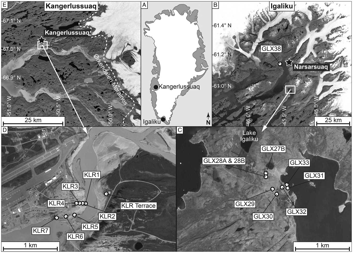
We specifically selected two field sites with very different geomorphic settings in order to test the ability of 10Be to date emergence, one in southern Greenland (Narsarsuaq/Igaliku) and the other in western Greenland (Kangerlussuaq) (Fig. 1). Both sites are underlain by quartz-rich, gneissic bedrock providing sufficient quartz for the extraction of 10Be. Previous 10Be measurements near both sites and made for the purpose of dating glacial retreat are consistent with erosive, warm-based ice removing most nuclides produced during previous interglacial periods (Levy al., 2012; Carlson et al., Reference Carlson, Winsor, Ullman, Brook, Rood, Axford, LeGrande, Anslow and Sinclair2014; Nelson et al., Reference Nelson, Bierman, Shakun and Rood2014).
Sample locations. (A) Index map. (B) Narsarsuaq/Igaliku region showing gravel beach berm sample (GLX38) that represents marine limit. (C) Expansion of panel B showing samples at Igaliku used to determine deglacial age and emergence history. (D) Kangerlussuaq area showing KLR sample locations along the Watson River. (E) Kangerlussuaq area and present ice margin with inset showing location of panel D. Dashed white line shows the approximate location of Ørkendalen moraine dated at 6.8±0.3 ka (Levy et al., Reference Levy, Kelly, Howley and Virginia2012).

At Kangerlussuaq, the current winter climate is very dry, and monthly snowfall during winter (in water equivalent) is on the order of only a centimeter or two. Narsarsuaq/Igaliku has a wetter climate, with up to 4 cm water equivalent falling per winter month. At neither site is the current winter snowfall sufficient, even if it did not melt over the 6 winter months, to cause more than percent-level differences in annual 10Be production under snow (maximum annual average shielding of 12 g/cm2); although there are data suggesting that snowfall may have been higher in the mid-Holocene (Thomas et al., Reference Thomas, Briner, Ryan-Henry and Huang2016).
Southern Greenland, Narsarsuaq/Igaliku area
In Igaliku/Narsarsuaq (southern Greenland), we collected samples from nine different sites in order to estimate the age of deglaciation and the relative sea-level fall that followed (Figs. 2 and 3). The landscape is dominated by deep fjords incised into the uplands; most bedrock is quartz-bearing, although there are outcrops of feldspar-dominated rocks (nepheline syenites) in which quartz is absent. A regional compilation of radiocarbon ages (both above and below the marine limit) suggests deglaciation of our field area at or before 9.7 cal ka BP (Weidick et al., Reference Weidick, Kelly and Bennike2004). A basal AMS radiocarbon age of a macrofossil (8920±190 14C yr BP, Poz-31634; cal age, 9540–10,430 cal yr BP, 2σ range) in a lake core collected from nearby Lake Igaliku (Fig. 1C) indicates deglaciation at our primary field site before 10.4 cal ka BP (Massa et al., Reference Massa, Perren, Gauthier, Bichet, Petit and Richard2012).
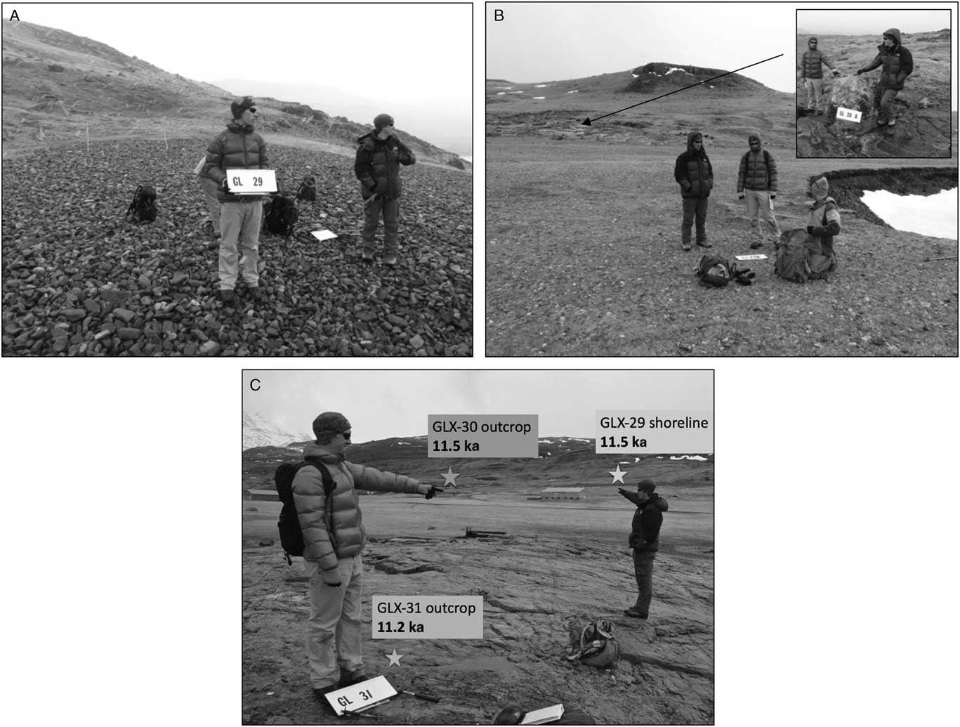
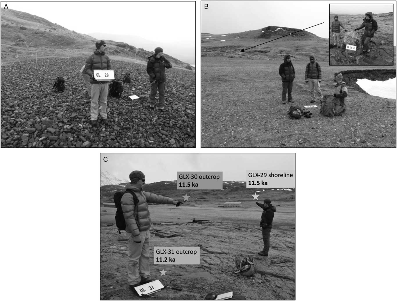
Narsarsuaq/Igaliku sample sites. (A) Cobble beach ridge (shoreline), GLX29, with age of 11.5±0.4 ka (1 standard error [SE] of cobbles, n=6) is marine limit in town of Igaliku. (B) Beach berm (GLX27; 11.5±0.1 ka, 1 SE of cobbles, n=9) is marine limit to the north of Igaliku. Inset shows boulder/bedrock pair (GLX28) above marine limit that dates local deglaciation to 11.4±0.3 ka (1 standard deviation analytic uncertainty). (C) Overview looking from near fjord (GLX31) toward a sampled outcrop (GLX30) and beach ridge (shoreline) that defines the local marine limit (GLX29, panel A).
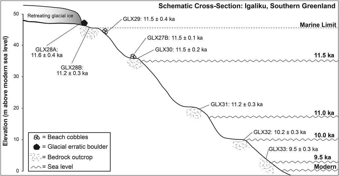
Schematic cross section at Igaliku showing sample sites, 10Be exposure ages, surveyed elevations, and sea level over time. Uncertainties are 1 standard error for cobble beaches and 1 standard deviation, internal error for bedrock outcrops and the boulder.

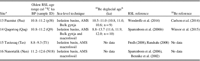
Previously published cosmogenic 10Be deglacial exposure ages in the region are older than most radiocarbon ages of organic material collected above the marine limit. Lowland moraine boulders in Narsarsuaq give four ages of 11.3±0.2 ka (Carlson et al., Reference Carlson, Winsor, Ullman, Brook, Rood, Axford, LeGrande, Anslow and Sinclair2014), older than the deglaciation of the valley upstream from Narsarsuaq (10.5±0.5 ka, n=10, bedrock and boulder samples) (Nelson et al., Reference Nelson, Bierman, Shakun and Rood2014). Qaqortoq, 70 km to the south, was deglaciated between 11.6 and 12.0 ka (n=10; Table 1) (Winsor et al., Reference Winsor, Carlson, Caffee and Rood2015).
South Greeenland emergence records and cosmogenic deglacial chronology comparison—Narsarsuaq/Igaliku.

Note: AMS, accelerator mass spectrometry; RSL, relative sea level.
a Numbering from Lecavalier et al. (Reference Lecavalier, Milne, Simpson, Wake, Huybrechts, Tarasov and Kjeldsen2014).
b Range of reported ages with mean, median, and error-weighted average in parentheses including total number of samples excluding samples identified by authors as outliers.
At four sites near where we collected samples (Table 1), emergence curves have been constructed using radiocarbon dating of organic material both from shorelines and from isolation basins (Lecavalier et al., Reference Lecavalier, Milne, Simpson, Wake, Huybrechts, Tarasov and Kjeldsen2014). At Paamiut, 300 km northwest of where we sampled, there was 50 m of emergence between 10.9 and 9.5 cal ka BP (Woodroffe et al., Reference Woodroffe, Long, Lecavalier, Milne and Bryant2014). At Qaqortoq, 70 km south of where we sampled, isolation basins indicate deglaciation at 11 cal ka BP and more than 30 m of emergence before current sea level was reached about 8.8 cal ka BP (Sparrenbom et al., Reference Sparrenbom, Bennike, Björck and Lambeck2006b). Isolation basin sampling at Nanortalik suggests deglaciation and emergence from 12.6 to 11.2 cal ka BP (Sparrenbom et al., Reference Sparrenbom, Bennie, Bjorck and Lambeck2006a); whereas at Tasiusaq emergence ages are much younger, 9.3–8.8 cal ka BP (Randsalu, Reference Randsalu2008). The first two sites have cosmogenic deglacial exposure ages that agree broadly with the basal radiocarbon age of the highest isolation basin (Table 1). At Paamiut, the cosmogenic and 14C age estimates for deglaciation overlap; at Qaqortoq, the cosmogenic age estimate (depending on the metric used to establish the deglacial age) is 600 to 1000 yr older than the central tendency of the 14C deglacial age estimate. We have not been able to find published cosmogenic data from Tasiusaq or Nanortalik.
In Igaliku, where we collected most of our samples, the highest postglacial sea level, the marine limit, is clearly defined by flat-topped, gravelly relict beach ridges surrounding the harbor area at the head of the fjord. Above the marine limit, there are glacially molded outcrops and erratic boulders. Below the marine limit, there are extensive outcrops of hard, minimally weathered rock. In coves, active, contemporary gravel beach ridges are common and extend several meters above modern high water levels. Tidal range in the area is only several meters.
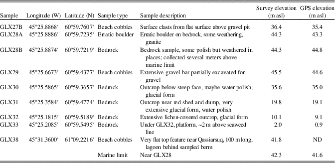
We collected samples both to date deglaciation and define the emergence history. To date deglaciation at Igaliku, we sampled (June 2011) an erratic boulder (GLX28A) and the glacially sculpted bedrock surface (GLX28B) on which the boulder sat, just above a beach ridge (GLX29) that defines the local postglacial marine limit. Below another beach ridge (GLX27B), we sampled four outcrops (GLX30–33) at different elevations above contemporary sea level (Figs. 2 and 3) to date emergence. We also sampled a third gravel beach ridge (GLX38) that defines the postglacial marine limit near Narsarsuaq about 30 km away. At each beach ridge, we collected numerous 5- to 10-cm-long cobbles and extracted quartz independently from each cobble. From outcrops, we collected thin surface samples (centimeter scale) using a hammer and chisel. In September 2012, we measured sample site locations precisely, including elevation, using both optical total station surveying tied to Danish benchmarks and Trimble PROXH GPS surveying using extended collection times and postprocessing (Table 2).
Sample site and location data for GLX sample series.

Notes: GPS location from Garmin 12, uncorrected. WGS 84. GPS elevation from Trimble ProXH with external antenna, postprocessed. Survey elevation from total station survey using benchmarks 81821 and 81516. m asl, meters above sea level; ND, no data.
Because inundation of outcrops during storms is only a small percentage of total exposure time, storm waves and high tides have an insignificant effect on the ages we calculate both for the marine limit and for progressively lower outcrops exposed as relative sea level fell. The paucity of till in much of Greenland, the openwork nature of the beach deposits, and the flat upper surface of the beach ridges we sampled argue against significant surface cover that is now eroded.
Western Greenland, Kangerlussuaq area
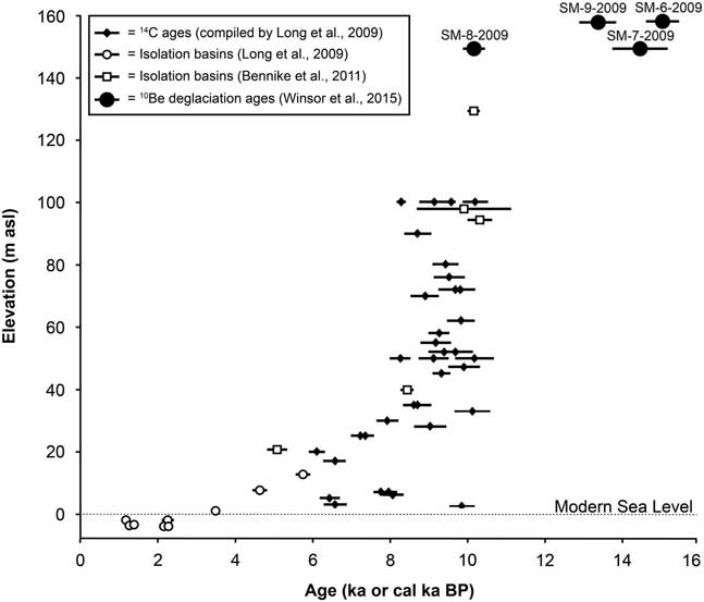
In western Greenland, for both inner and outer Kangerlussuaq Fjord, emergence curves based on radiocarbon dating of sediment were constructed first in the 1970s (Ten Brink, Reference Ten Brink1974) and updated recently (Storms et al., Reference Storms, de Winter, Overeem, Drijkoningen and Lykke-Andersen2012). There are additional data near the mouth of the fjord collected from isolation basins (Long et al., Reference Long, Woodroffe, Dawson, Roberts and Bryant2009, Reference Long, Woodroffe, Roberts and Dawson2011; Bennike et al., Reference Bennike, Wagner and Richter2011). The isolation basin data provide a coherent view of emergence history with emergence prevailing from deglaciation until the late Holocene (3 cal ka BP) when submergence began in response to Neoglacial ice advance (Fig. 4).
Example of western Greenland emergence information compiled along with 10Be deglacial ages. Plot incorporates calibrated radiocarbon ages of marine organic material related to sea level (black diamonds) as well as isolation basin estimates of past sea levels (open symbols) and cosmogenic 10Be exposure ages for boulders. Data from Long et al. (Reference Long, Woodroffe, Dawson, Roberts and Bryant2009), Bennike et al. (Reference Bennike, Wagner and Richter2011), and Winsor et al. (Reference Winsor, Carlson, Caffee and Rood2015).
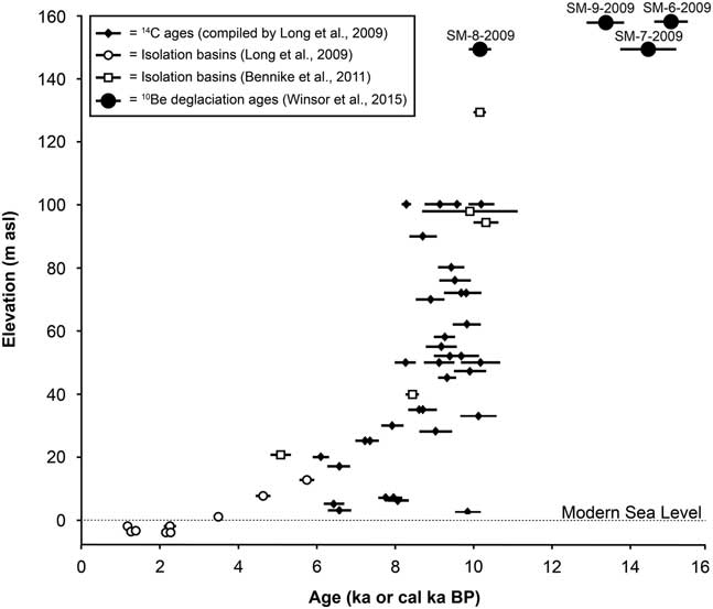
However, a compilation (Long et al., Reference Long, Woodroffe, Dawson, Roberts and Bryant2009) of previously published radiocarbon ages for emergence in the Sismiut area (western Greenland ~160 km from our sample site at Kangerlussuaq and close to the mouth of the fjord) illustrates the uncertainty of radiocarbon-based emergence curves. In the Sismiut data set, there is a 20% range in calibrated ages for samples collected at the same elevation (~100 m, the marine limit), as well as 8–10 cal ka BP ages in deposits sampled at many elevations between present-day sea level and the marine limit (Fig. 4). These calibrated radiocarbon ages, along with ages published later (Bennike et al., Reference Bennike, Wagner and Richter2011), are systematically less than most 10Be exposure ages in the area that have been interpreted as indicating deglaciation at about 14.5 ka (Winsor et al., Reference Winsor, Carlson, Caffee and Rood2015), although the radiocarbon ages that define rapid early emergence match well with the youngest 10Be exposure age considered an outlier by Winsor et al. Such an offset between the methods could indicate that the 10Be ages are systematically too old (because of the presence of inherited nuclides; Briner et al., Reference Briner, Goehring, Mangerud and Svendsen2016) or that 14C ages are too young (because of delayed accumulation of organic material after deglaciation and/or emergence; Davis and Davis, Reference Davis and Davis1980). Offsets between organic radiocarbon ages of deglaciation and those estimated by cosmogenic nuclides such as 10Be have been noted before and can exceed 1000 yr (Larsen et al., Reference Larsen, Funder, Kjær, Kjeldsen, Knudsen and Linge2014).
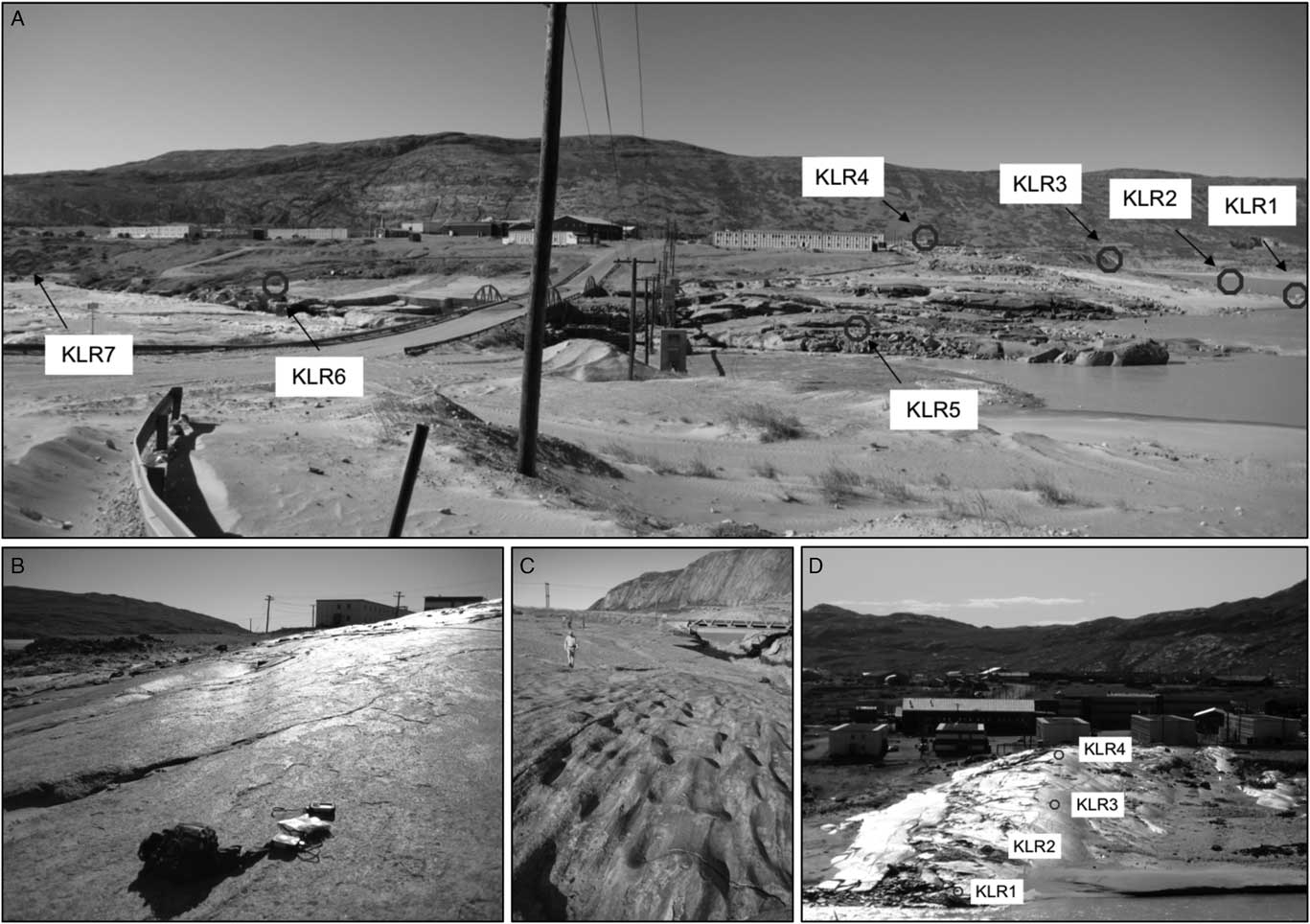
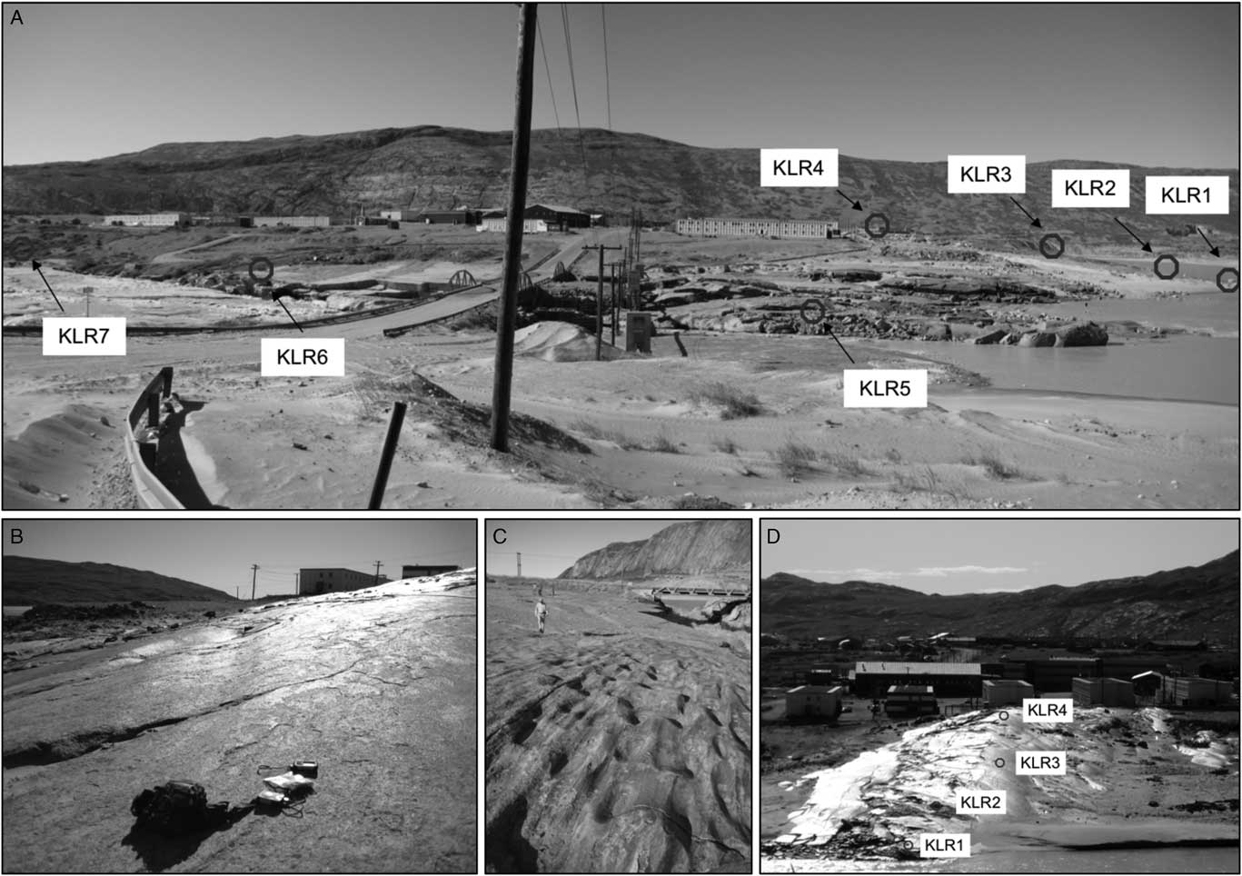
At Kangerlussuaq, during July 2008, we collected seven samples to determine the Watson River’s incision history, which we believe reflects isostatic uplift as ice retreated inland during the middle Holocene (Fig. 5). The town of Kangerlussuaq is located on a flat-topped, valley-filling landform composed of bedded sand and gravel termed the Keglen Delta, deposited between 6.5 and 7.1 cal ka BP (based on 14C dating; Storms et al., Reference Storms, de Winter, Overeem, Drijkoningen and Lykke-Andersen2012). Erosion of this thick blanket of unconsolidated sediment by the Watson River has exposed a bedrock ridge normal to river flow (Figs. 5 and 6). This bedrock was glacially rounded and polished by ice flow before deglaciation, the timing of which was 10Be exposure dated (Levy et al., Reference Levy, Kelly, Howley and Virginia2012) at >6.8±0.3 ka (n=10, age of Ørkendalen moraines upstream). At the top of the ridge, deep glacial grooves are preserved, and there is no evidence for fluvial erosion. Lower on the ridge, closer in elevation to the river, evidence for glaciation has been overprinted by fluvial processes; specifically, the bedrock has been eroded and fluted by sediment-laden river water.
Kangerlussuaq sample sites. (A) Overview showing samples KLR1 to KLR4 along bedrock ridge exposed as terrace sediments (on which buildings sit) were incised by Watson River (shown to right and along front of image). Samples KLR5, KLR6, and KLR7 on strath terrace. Field of view about 700 m. (B) Glacial groove exposed by removal of terrace sediment at KLR3, field gear for scale. (C) Strath terrace with flow features, sample location KLR6, person for scale. (D) Oblique view showing vertical transect of sample sites KLR1 to KLR4.
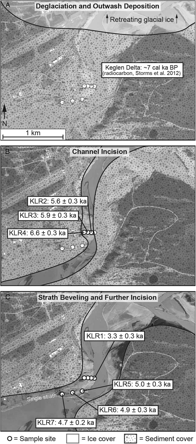
Map view (Google Earth) of Kangerlussuaq sample sites showing 10Be ages and inferred history of ice retreat (A), channel incision (B), and strath terrace beveling as indicated by three similar exposure ages on the bedrock strath terrace (C).

Downstream from the ridge and immediately adjacent to the estuary is a bare bedrock strath terrace, a several-hundred-meter-long, smooth, flat, bedrock surface shaped by fluvial erosion. The present-day channel of the Watson River is incised into this surface, and except for summer floods, the strath terrace is high and dry above the channel and thus currently inactive and relict. The terrace bedrock surface is heavily fluted and potholed indicating it was sculpted by flowing water and sediment rather than by ice (Fig. 5C); that sediment now blankets the fjord bottom downstream. Strath terraces such as this are thought to form when river grade (slope) is stable and lateral planation rather than incision dominates; thus, they indicate relative stability of base level and here, a slowing or cessation of uplift and incision.
We collected four samples from hard, polished bedrock surfaces at different elevations along the bedrock ridge and three samples from the strath terrace parallel to the Watson River channel (Figs. 5 and 6); all of these samples once lay below a thick blanket (meters to tens of meters) of Keglen Delta sediment and so were shielded from cosmic radiation until incision and removal of the material by the downcutting Watson River sequentially exposed the sampling sites. This incision was in response to uplift-induced, relative base-level lowering in the nearby fjord (Storms et al., Reference Storms, de Winter, Overeem, Drijkoningen and Lykke-Andersen2012) and not to changes in eustatic sea level, which was relatively stable by the mid-Holocene. Such uplift would have been the result of the Greenland Ice Sheet retreating inland of its current position after 6.8 ka during the mid-Holocene thermal optimum (Levy et al., Reference Levy, Kelly, Howley and Virginia2012).
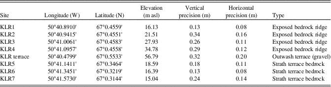
We used a Trimble PROXH GPS in 2011 with extended collection times and postprocessing to establish precise elevation control and sample location (<1 m uncertainty; Table 3). Our expectation in sampling was that samples lower on the ridge were exposed later than those higher on the ridge and that the age of the strath terrace would reflect a time when base level became stable because isostatic uplift slowed or ceased.
Sample site and location data for KLR samples and terrace.

Notes: Field data collected using Trimble ProXH unit with external antenna. Postprocessed against Kellyville base station using Hstar correction. WGS84. m asl, meters above sea level.
ANALYTICAL METHODS
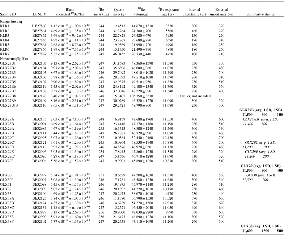
Samples were processed at the University of Vermont using standard methods (Corbett et al., Reference Corbett, Bierman and Rood2016c). All samples were ground, and the 250–850 µm fraction was retained. We ground each cobble in its entirety because cobbles were irregularly shaped and we do not know their stirring history. After quartz was separated and purified, beryllium was isolated in batches of 12 samples (GLX, 7 batches, 8 blanks; KLR, 1 batch, 8 associated blanks; Table 4). Samples were measured using AMS at Lawrence Livermore National Laboratory (Rood et al., Reference Rood, Hall, Guilderson, Finkel and Brown2010, Reference Rood, Brown, Finkel and Guilderson2013). A blank correction, based on the average measured 10Be/9Be ratio of all blanks (and the standard deviation [SD]) measured with each group of samples, was applied, and errors were propagated in quadrature. Analyses were normalized to the 07KNSTD standard series (Nishiizumi et al., Reference Nishiizumi, Imamura, Caffee, Southon, Finkel and McAninch2007). We made three replicate analyses (for samples GLX29C, 29E, and 30) using separate quartz aliquots (Table 4). Considering only internal errors (AMS counting statistics), two replicates gave similar concentrations at 1σ; the other replicate agreed at 2σ. We used the average value for each replicated sample in our data analysis. One sample, GLX27B8, provided a small amount (5 g) of impure quartz (>1000 ppm 27Al). It had a 10Be concentration two times that of the other samples from site GLX27B perhaps because of the inclusion of other mineral phases high in 10Be or because of inheritance. It was removed from further calculations as an outlier.
Cosmogenic isotopic data, Greenland emergence.

Notes: All analyses normalized to 07KNSTD standards as per values in Nishiizumi et al. (Reference Nishiizumi, Imamura, Caffee, Southon, Finkel and McAninch2007). GLX measured isotope ratios corrected using multiple full process blanks measured with samples (n=8, 5.6±2.9×10⁻¹⁶). KLR measured isotope ratios corrected using multiple full process blanks measured with samples (n=8, 3.5±1.5×10⁻¹⁶). One of 22 cobbles is an outlier (GLX27B8), with an age of 25.31 ky; we omit it from the calculations. Age calculations done with CRONUS, NENA (Greenland production rate, calculator version 2.1, wrapper script 2.2, constants 2.2.1, muons 1.1). Average age for beach cobbles shown in bold with 1 standard deviation (SD), 1 standard error (SE); LLNL, Lawrence Livermore National Laboratory.
a Replicate analysis using distinct quartz aliquot; averages and SD shown in italics.
We calculated exposure ages and external uncertainties (considering scaling and production rate in addition to analytical precision) using the CRONUS calculator (Balco et al., Reference Balco, Stone, Lifton and Dunai2008) (main calculator version 2.1, wrapper script 2.2, constants 2.2.1, muons 1.1) using the Arctic production rate (Young et al., Reference Young, Schaefer, Briner and Goehring2013), Lal/Stone scaling, and a time-invariant nuclide production rate. For the CRONUS calculator, we assumed a thickness of 2.5 cm (average intermediate cobble axis, 5 cm), which is appropriate if the cobbles were stirred over time (which we expect because of frost heaving and bioturbation).
Our measurements of 10Be are precise (median 1σ precision <3%), which allows us to define closely (within 200-300 yr, internal error) the relative timing of beach gravel deposition and exposure of outcrops as they emerged from beneath water in the Narsarsuaq/Igaliku area and from beneath sediment in Kangerlussuaq. External errors, considering the imprecision in nuclide production rate calibration and appropriate for comparing cosmogenic ages with radiocarbon ages, are larger by a factor of about 2, averaging ~500 yr. We did not make a correction for elevation change attributable to isostatic uplift after exposure because the resulting changes in production rates are much smaller than the errors (both random and systematic) in our reported ages. All uncertainties in 10Be concentrations are reported as 1 SD of the analytic uncertainty only. For ages, we report both internal uncertainties (analytic) and external (considering production rate uncertainty). For ages of cobble beaches, we report the mean and 1 standard error (SE) considering the number of clasts analyzed and included in the mean.
RESULTS AND INTERPRETATION
Southern Greenland
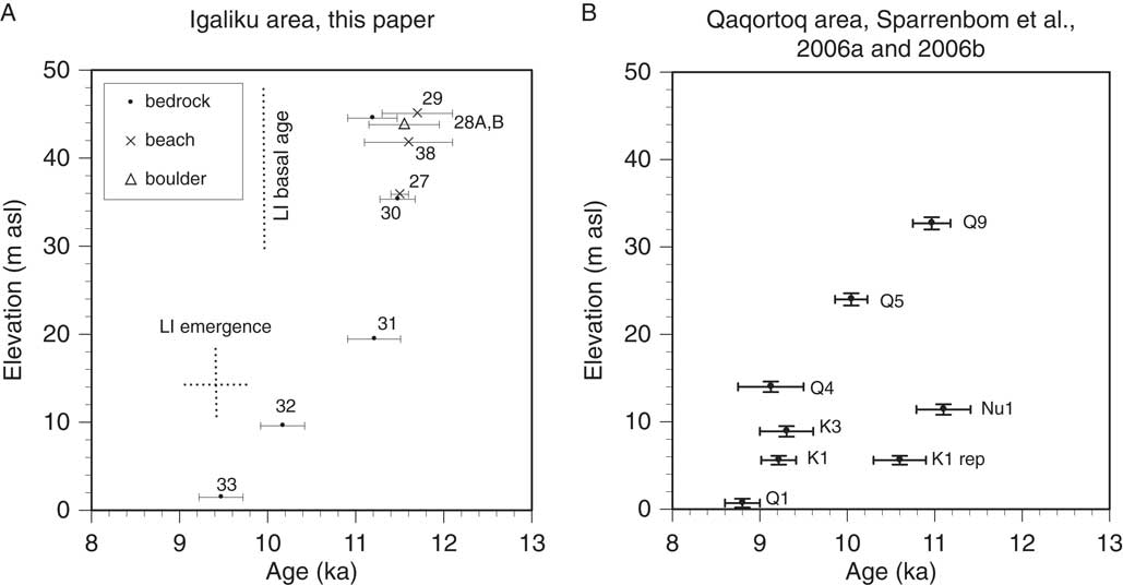
The Narsarsuaq/Igaliku record, from southern Greenland, spans 1900 yr after deglaciation at ~11.4 ka (the average of boulder/bedrock pair exposure ages, GLX28A and B) and until the exposure of the lowest sample (GLX33) near present-day high water at 9.5 ka. The three beach ridges, which represent the local marine limit (Table 2), have statistically indistinguishable ages (mean±1 SE) considering the age of numerous cobbles collected and analyzed from each beach ridge (11.5±0.1 ka, n=9, GLX27B, 36 meters above sea level [m asl]; 11.6±0.5 ka, n=6, GLX38, 42 m asl; and 11.5±0.4 ka, n=6, GLX29, 45 m asl) despite being separated by more than 30 km (Fig. 7, Table 4). The range of beach ridge ages for the marine limit (11.5 to 11.6 ka) overlaps the deglaciation age defined by the mean of the age of the dated bedrock/erratic boulder pair (11.4±0.3 ka [1 SD], GLX28A and B, 45 m asl) above the local marine limit as defined by those same beach deposits. The beaches were deposited immediately after deglaciation.
Emergence curves, southern Greenland. (A) Narsarsuaq/Igaliku emergence curve derived from 10Be measurements (numbers are sample GLX ID) of erratic boulder and glaciated bedrock above marine limit (GLX28), cobble beaches at marine limit (GLX27, 29, 38), and outcrops exposed as relative sea level fell (GLX30,31,32,33). “LI emergence” is the reported elevation and age of Lake Igaliku emergence (15 m, ~9.5 ka) (Massa et al., Reference Massa, Perren, Gauthier, Bichet, Petit and Richard2012). “LI basal age” is reported at ~10 ka cal 14C (Massa et al., Reference Massa, Perren, Gauthier, Bichet, Petit and Richard2012) and appears to be too young by about 1.5 ka. Uncertainty of LI emergence (LIE) elevation and age is not known but suggested by dashed lines. Elevation uncertainty for 10Be samples is smaller than symbol and therefore not shown. Age uncertainty shown at 1 standard error for cobble beaches and internal uncertainty for other samples. (B) Qaqortoq area emergence data (calibrated 14C ages) from Sparrenbom et al. (Reference Sparrenbom, Bennie, Bjorck and Lambeck2006a, Reference Sparrenbom, Bennike, Björck and Lambeck2006b).
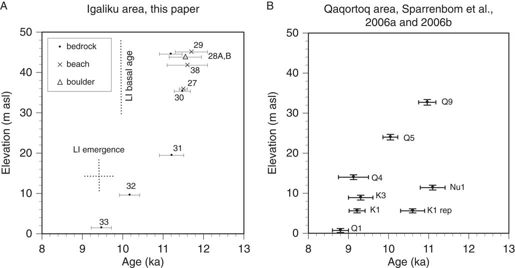
The samples we collected and dated reflect 45 m of relative sea-level fall (Figs. 3 and 7) similar in timing and magnitude to other south Greenland emergence curves (Bennike et al., Reference Bennike, Björck and Lambeck2002; Sparrenbom et al., Reference Sparrenbom, Bennike, Björck and Lambeck2006b, Reference Sparrenbom, Bennike, Fredh, Randsalu-Wendrup, Zwartz, Ljung, Björck and Lambeck2013) and the ~50 m emergence inferred previously for the Narsarsuaq/Igaliku area (Weidick et al., Reference Weidick, Kelly and Bennike2004; Long et al., Reference Long, Woodroffe, Roberts and Dawson2011). The exposure ages of four outcrops (from just below the elevation of the gravel beach to just above the present-day high waterline) are in stratigraphic order (GLX30, 35 m asl, 11.5 ka; GLX31, 19 m asl, 11.2 ka; GLX32, 10 m asl, 10.2 ka; and GLX33, 1.5 m asl, 9.5 ka) from which we conclude that relative sea level fell rapidly in the early Holocene, reaching its current level by 9.5 ka, similar to the ~8.8 cal ka BP inferred from local (Sparrenbom et al., Reference Sparrenbom, Bennike, Björck and Lambeck2006b) and regional (Woodroffe et al., Reference Woodroffe, Long, Lecavalier, Milne and Bryant2014) isolation basin studies.
The high spatial and temporal resolution of the 10Be record demonstrates that initial sea-level fall was extremely fast, about 25 m in at most a few hundred years, similar to the rapid, immediately postglacial emergence inferred with fewer data (from bivalves in sediment) in western Greenland (Ten Brink, Reference Ten Brink1974) and in southern Greenland (Woodroffe et al., Reference Woodroffe, Long, Lecavalier, Milne and Bryant2014) using isolation basins. Local sea level, immediately adjacent to a large (Washburn, Reference Washburn1962) and shrinking ice sheet, can fall with exceptional rapidity as the local gravitational field changes substantially when the ice sheet ablates and when the underlying rock responds elastically (Ten Brink, Reference Ten Brink1974; Clark, Reference Clark1976).
This rapid emergence means that the time any sample site spent under shallow water prior to subaerial exposure was minimal and thus had little if any influence on calculated exposure ages. The Narsarsuaq/Igaliku data provide strong evidence that rapid melting of the ice sheet in part drove initial emergence through changes in the local gravitational field (Clark, Reference Clark1976), and the timing is consistent with large volumes of ice loss driven by abrupt warming immediately following the Younger Dryas; such rapid ice loss may have influenced later patterns of ice loss (Gomez et al., Reference Gomez, Mitrovica, Huybers and Clark2010). Applying a global eustatic correction attributable to melting ice sheets (Lambeck et al., Reference Lambeck, Rouby, Purcell, Sun and Sambridge2014) of 15 m/ka suggests total uplift and gravity driven sea-level fall during the 1900 yr emergence period recorded by 10Be of ~75 m. Glaciologic modeling of uplift in the region (Qaqortoq) matches poorly our data and those of others (Woodroffe et al., Reference Woodroffe, Long, Lecavalier, Milne and Bryant2014); observed uplift (Fig. 7) is much more rapid than modeled uplift (Lecavalier et al., Reference Lecavalier, Milne, Simpson, Wake, Huybrechts, Tarasov and Kjeldsen2014).
The new cosmogenic ages for deglaciation agree with others in the region (when all ages are calculated the same way using the same production rate and are thus directly comparable). For example, our cosmogenic estimate of deglaciation (11.4±0.3 ka, n=2, GLX28A, B) near sea level at Igaliku is indistinguishable from the estimate 30 km north in Narsarsuaq (11.3±0.2 ka, n=4) made on the basis of lowland morainal 10Be exposure ages (Carlson et al., Reference Carlson, Winsor, Ullman, Brook, Rood, Axford, LeGrande, Anslow and Sinclair2014). Igaliku deglaciation likely postdates ice leaving Qaqortoq 70 km southeast (Winsor et al., Reference Winsor, Carlson, Caffee and Rood2015) ~12 ka (n=10; Table 1) but predates deglaciation (Nelson et al., Reference Nelson, Bierman, Shakun and Rood2014) of the valley upstream from Narsarsuaq (10.5±0.5 ka, n=10).
However, the new 10Be ages are older than most deglacial and emergence ages determined from radiocarbon analysis of organic material in nearby lake cores. For example, our 10Be deglaciation estimate of 11.4±0.3 ka is about 1.7 ka older than a previous (9.7 cal ka BP) regional estimate of deglaciation (Weidick et al., Reference Weidick, Kelly and Bennike2004) and 1.4 ka older than the central tendency of the basal lake sediment macrofossil radiocarbon age (9.5–10.4 cal ka BP, 2 SD) of a core collected from nearby (Fig. 1C) Lake Igaliku (Massa et al., Reference Massa, Perren, Gauthier, Bichet, Petit and Richard2012). The emergence of the Lake Igaliku basin (stated elevation 15 m, from low-resolution topographic map; Massa et al., Reference Massa, Perren, Gauthier, Bichet, Petit and Richard2012) at 9.5 cal ka BP is similarly young in comparison to the 10Be-determined emergence curve we generated (Fig. 7). In contrast, our new Igaliku record of emergence is similar in timing and emergence magnitude (Fig. 7) to that generated 70 km south in Qaqortoq (Sparrenbom et al., Reference Sparrenbom, Bennike, Björck and Lambeck2006b). They differ in that the new Igaliku record has tighter elevation control, data from the initial 15 m of emergence, and no inconsistent data (such as Nu1, Q4, and K1 rep; Fig. 7B).
There are three possible explanations for what appears to be offset between organic radiocarbon ages and cosmogenic exposure ages at some sites, including Igaliku: (1) The 10Be production rate in use is too low causing exposure ages to be too old. (2) All samples contain 10Be inherited from prior exposure, but 10Be production rate calibration samples do not. (3) The radiocarbon ages with which we and others compare our 10Be ages are too young (Larsen et al., Reference Larsen, Funder, Kjær, Kjeldsen, Knudsen and Linge2014). Below we explore each of these explanations.
We consider it improbable that all cosmogenic samples we report here as well as those analyzed in the area by others (Carlson et al., Reference Carlson, Winsor, Ullman, Brook, Rood, Axford, LeGrande, Anslow and Sinclair2014; Nelson et al., Reference Nelson, Bierman, Shakun and Rood2014; Winsor et al., Reference Winsor, Carlson, Caffee and Rood2015) are systematically too old because the production rate used for calculation is too low. We reject production rate inaccuracies (which would need to be ~10%) as explanation for the 10Be/organic radiocarbon dating mismatch because the 10Be production rate we and others use to interpret our Greenland data is locally calibrated. The 10Be production rate was determined over a similar time scale and at a similarly high latitude and low elevation (Briner et al., Reference Briner, Young, Goehring and Schaefer2012) as these samples. Furthermore, because samples for both dating (Carlson et al., Reference Carlson, Winsor, Ullman, Brook, Rood, Axford, LeGrande, Anslow and Sinclair2014; Nelson et al., Reference Nelson, Bierman, Shakun and Rood2014; Winsor et al., Reference Winsor, Carlson, Caffee and Rood2015) and production rate were collected at high latitudes (Briner et al., Reference Briner, Young, Goehring and Schaefer2012), varying magnetic field strength over time cannot influence production rates.
Although nuclides can be inherited from previous periods of exposure at and near Earth’s surface, as shown for samples in southern Norway (Briner et al., Reference Briner, Goehring, Mangerud and Svendsen2016) and in northern Greenland (Corbett et al., Reference Corbett, Bierman, Graly, Neumann and Rood2013), we consider such inheritance an unlikely explanation for the offset between radiocarbon and 10Be age estimates for several reasons. Most importantly, inheritance has been found in many cosmogenic studies in glaciated terrains, but it has never been uniform; boulders and outcrops carry different concentrations of inherited nuclides reflecting different prior exposure and erosion histories (Corbett et al., Reference Corbett, Bierman and Rood2016a). In Igaliku, the similarity in ages between multiple beach cobbles and between bedrock and boulder ages in this and other nearby glacial dating campaigns (Carlson et al., Reference Carlson, Winsor, Ullman, Brook, Rood, Axford, LeGrande, Anslow and Sinclair2014; Nelson et al., Reference Nelson, Bierman, Shakun and Rood2014; Winsor et al., Reference Winsor, Carlson, Caffee and Rood2015) would require extremely uniform inheritance, with a variance between dozens of samples of only a few hundred years of exposure equivalent; we consider that unlikely.
Furthermore, cobbles collected directly from the Greenland Ice Sheet along its western margin have a median 10Be concentration of only about 1000 atoms/g, the equivalent of at most several hundred years of surface exposure (Corbett et al., Reference Corbett, Bierman, Neumann and Graly2016b), far less than reported for the inheritance in Norwegian samples (Briner et al., Reference Briner, Goehring, Mangerud and Svendsen2016). Such low inheritance is likely both the result of shorter interglacial exposure around Greenland than in southern Norway and the persistence of the Greenland Ice Sheet over millions of years (Bierman et al., Reference Bierman, Shakun, Corbett, Zimmerman and Rood2016). Because the ages we calculate from cobbles on beach deposits and those we calculate from bedrock and an overlying erratic boulder agree at 1 SD, we infer that none of these samples likely carries more than a few hundred years of surface equivalent muon-produced 10Be. This is a small portion (<20%) of the concentration of 10Be needed to reconcile the radiocarbon and 10Be age estimates for deglaciation and emergence.
We suspect that the offset in southern Greenland between some radiocarbon-based chronologies and cosmogenic ages (Carlson et al., Reference Carlson, Winsor, Ullman, Brook, Rood, Axford, LeGrande, Anslow and Sinclair2014; Nelson et al., Reference Nelson, Bierman, Shakun and Rood2014; Winsor et al., Reference Winsor, Carlson, Caffee and Rood2015), including those reported here, mostly reflects a young bias in radiocarbon ages at deglaciation and during early emergence. Considering the evidence presented previously, we suspect that many radiocarbon ages are too young because they reflect a lag time after deglaciation, before sufficient organic material accumulated for dating (Davis and Davis, Reference Davis and Davis1980). Such ages, whether derived from samples collected from lake sediment cores or from marine sediment, therefore represent minimum limits on deglaciation and emergence. The challenge of finding deglacially contemporaneous organic material is especially acute in ice marginal areas in the Arctic during the Pleistocene where climate remained cold after deglaciation. During the Holocene, once climate was warmer and vegetation had become reestablished, the offset between 10Be and radiocarbon ages should be and is usually less or nonexistent (Briner et al., Reference Briner, Stewart, Young, Philipps and Losee2010).
Western Greenland
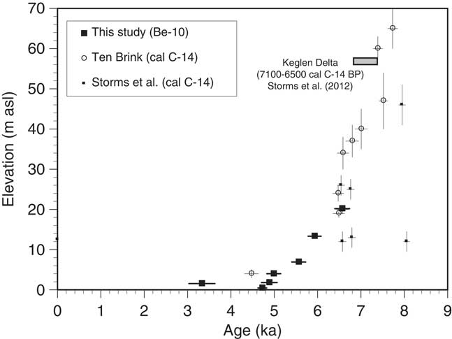
The relative sea-level record at Kangerlussuaq, western Greenland, which is otherwise well constrained (Ten Brink, Reference Ten Brink1974; Storms et al., Reference Storms, de Winter, Overeem, Drijkoningen and Lykke-Andersen2012) by radiocarbon dating of marine mollusks in sediment (Ten Brink, Reference Ten Brink1974), has a gap in the middle Holocene when ice retreated beyond the current margin. Our new 10Be data span 3.2 ka and 18.5 m of emergence in the later Holocene and fill this gap (Fig. 8, Table 4). In Kangerlussuaq, the 10Be exposure ages are younger than in the Narsarsuaq/Igaliku area because glacial retreat occurred later (10Be age, Ørkendalen moraines [Levy et al., Reference Levy, Kelly, Howley and Virginia2012], 6.8±0.3 ka and 14C on bivalves in Keglen Delta proglacial sediment downstream, 6.5–7.1 cal ka BP [Storms et al., Reference Storms, de Winter, Overeem, Drijkoningen and Lykke-Andersen2012]).
Emergence curve for Kangerlussuaq, western Greenland. Includes existing 14C data (Ten Brink, Reference Ten Brink1974; Storms et al., Reference Storms, de Winter, Overeem, Drijkoningen and Lykke-Andersen2012) calibrated using CALIB and new 10Be exposure ages plotted using the relationship between their measured elevation and paleo–sea level at 4.5 ka. Keglen delta cal 14C age range (Ten Brink, Reference Ten Brink1974; Storms et al., Reference Storms, de Winter, Overeem, Drijkoningen and Lykke-Andersen2012) and elevation plotted. Age uncertainties plotted as 1 standard deviation internal error. Elevation uncertainty for 10Be samples is smaller than symbol and therefore not shown.

The oldest (6.6 ka, KLR04) and highest (35 m asl) of our Kangerlussuaq exposure ages indicates that incision of the Keglen Delta and exposure of bedrock in the Watson River valley began just after the Greenland Ice Sheet retreated from the Ørkendalen moraines at 6.8 ka (Table 4). Exposure ages lower on the bedrock ridge are in stratigraphic order, with a total of 18.5 m of incision beginning at 6.6 ka and ending at 3.3 ka when the Watson River stopped incising. Downstream, the river cut a broad strath terrace at ~4.8 ka (KLR5, 6, and 7). The terrace reflects decreasing incision rates as a result of increasing base level stability; such stability allowed the river to bevel the channel bed and create the strath terrace. The end of incision and emergence reflects Neoglacial ice readvance and consequent subsidence, which our data suggest started around 3.3 ka, similar to the ~4 cal ka BP age suggested by others for the region on the basis of calibrated radiocarbon ages (Weidick et al., Reference Weidick, Oerter, Reeh, Thomsen and Thorning1990; Weidick, Reference Weidick1993; van Tatenhove and van der Meer, Reference van Tatenhove and van der Meer1996; Wahr et al., Reference Wahr, van Dam, Larson and Francis2001).
Because our bedrock samples at Kangerlussuaq were exposed by erosion of the overlying sand and gravel as the Watson River incised, inferring changes over time in local relative sea-level elevation from sample elevation requires making assumptions about the relationship between the sample sites upstream of the fjord and local, relative sea level in the fjord. To do this, we presume that the Watson River has maintained a similar grade (water surface and channel bottom slope) over time and subtract the elevation offset between the ~4.8 ka strath terrace (18 m asl) and the 4.5 cal ka BP age of the 2 m asl sea level of Ten Brink (Ten Brink, Reference Ten Brink1974) from all our data. It is important to consider that our inferences about the timing of uplift, incision, and the end of emergence are independent of the assumptions about river grade and effective sample elevation.
10Be dating of late Holocene bedrock exposure along the Watson River provides new constraints on the timing and magnitude of neoglaciation in western Greenland. Considered along with the dating of the Ørkendalen and Keglen moraines near Kangerlussuaq (Levy et al., Reference Levy, Kelly, Howley and Virginia2012; Storms et al., Reference Storms, de Winter, Overeem, Drijkoningen and Lykke-Andersen2012; Carlson et al., Reference Carlson, Winsor, Ullman, Brook, Rood, Axford, LeGrande, Anslow and Sinclair2014; Winsor et al., Reference Winsor, Carlson, Caffee and Rood2015), the 10Be data suggest that the Greenland Ice Sheet was inland of the Ørkendalen margin to the east of Kangerlussuaq between ~6.8 ka and at least 3.3 ka (our youngest age, just above the low-flow channel margin). Uplift diminished and the strath terrace was cut by 4.8 ka as ice marginal retreat slowed and river incision slowed or ceased allowing lateral channel migration and bedrock strath planation. The 10Be data and uplift/relative sea-level inferences from them at Kangerlussuaq are consistent with isolation basin data from the Sisimiut area 150 km west (Long et al., Reference Long, Woodroffe, Dawson, Roberts and Bryant2009). There, relative sea level was +15 m at 5.7 ka (our estimate up fjord at Kangerlussuaq at that time is +16 m), and uplift at Sisimiut ended between 4 and 3 ka similar to our suggestion that uplift slowed by 4.8 ka and ended by 3.3 ka. Overall, 10Be data support the inference (from two lakes cored near the ice margin) that ice was behind the present-day margin near Kangerlussuaq between 5.8 and 1.8 ka (Young and Briner, Reference Young and Briner2015).
DISCUSSION
10Be dating of Greenlandic relative sea levels provides precise age/elevation data revealing both tens of meters of emergence in just a few centuries after deglaciation as well as the timing and geomorphic response to neoglaciation in the late Holocene. In southern Greenland, at Igaliku, cosmogenic dating of deglacial and emergence features shows that deglaciation and thus emergence were especially rapid after 11.4 ka. Systemic differences between cosmogenic and radiocarbon dating of this emergence appear during the first millennia or two after deglaciation when organic material was especially scarce (Davis and Davis, Reference Davis and Davis1980; Weidick et al., Reference Weidick, Kelly and Bennike2004) resulting in systematic prior underestimation of initial emergence rates and emergence age at Igaliku and likely elsewhere in southern Greenland. This interval is especially important to capture accurately in order to inform models simulating ice sheet response to past climate forcing. Such bias in dating could make ice sheets and the solid Earth appear to respond with a longer lag and more slowly to climate change than they actually do. At least some models constrained by 14C-based emergence curves appear to underestimate initial emergence rates (Lecavalier et al., Reference Lecavalier, Milne, Simpson, Wake, Huybrechts, Tarasov and Kjeldsen2014; Sinclair et al., Reference Sinclair, Carlson, Mix, Lecavalier, Milne, Mathias, Buizert and DeConto2016), as seen by comparing rapid initial emergence rates from the cosmogenic Narsarsuaq/Igaliku record with simulated emergence curves for many sites around Greenland (Lecavalier et al., Reference Lecavalier, Milne, Simpson, Wake, Huybrechts, Tarasov and Kjeldsen2014).
There are limitations to dating postglacial emergence with cosmogenic isotopes. The method will not provide accurate ages where relative sea level has risen after initially falling because there will be multiple periods of exposure interrupted by shielding under water (Stone et al., Reference Stone, Lambeck, Fifield, Cresswell and Evans1995). None of the sites we investigated in Greenland have experienced such complex emergence histories (Lecavalier et al., Reference Lecavalier, Milne, Simpson, Wake, Huybrechts, Tarasov and Kjeldsen2014). Accurate exposure dating can be prevented by nuclides inherited from prior periods of cosmic-ray exposure. For example, dating a series of nested cobble beaches is unlikely to produce interpretable data because cobbles with prior exposure histories from higher beach berms are likely to be reworked by storm waves into lower beach berms (Gosse et al., Reference Gosse, Hecht, Mehring, Klein, Lawn and Dyke1998; Briner et al., Reference Briner, Gosse and Bierman2006). In the example presented here, we sampled only the highest cobble beaches assuming that these cobbles were derived directly from glacial till and/or outwash and had no recent history of prior cosmic-ray exposure; this assumption is confirmed by their homogenous ages and the minimal offset between the beach ages and an adjacent erratic boulder and glacially scoured bedrock surface immediately above them. In principle, in situ produced 14C, with its short half-life could help address the issue of inheritance. Practically, such analyses are currently difficult to make, imprecise, and costly, and the production rates of this nuclide over time, space, and depth remain less certain than for 10Be.
The presence of warm-based, erosive ice is critical to the success of the method we propose. In areas where ice was cold based, erosion will be minimal and nuclides will be inherited from prior periods of exposure (Bierman et al., Reference Bierman, Marsella, Patterson, Davis and Caffee1999), which will confound the dating of emergence. Without removal of at least several meters of rock during the most recent glaciation, accurate dating of sea level using 10Be in outcrops would not be possible; even so, in areas where there are long interglacial periods of exposure, low rates of 10Be production by deeply penetrating muons may inflate calculated cosmogenic exposure ages (Briner et al., Reference Briner, Goehring, Mangerud and Svendsen2016), although we do not see that effect in the study areas considered here. We doubt that inheritance of nuclides from prior periods of exposure will be a significant limitation for application of the method except in areas where cold-based ice dominates, because large volumes of outwash, many deltas, and frequent glacially streamlined forms suggest that much ice near even high arctic coastlines, at least at in large fjords, was warm based (Roberts and Long, Reference Roberts and Long2005). The low median 10Be concentration in ice-sourced Greenlandic cobbles (Corbett et al., Reference Corbett, Bierman, Neumann and Graly2016b) suggests that marine limit beach deposits are likely to be amenable to dating even if lower and younger beach deposits are not (Briner et al., Reference Briner, Gosse and Bierman2006).
CONCLUSIONS
Data we present here demonstrate the precision and utility of a widely applicable technique for establishing emergence rates along previously glaciated coastlines. Here, we show that sites can be selected to minimize inheritance of cosmogenic nuclides from prior periods of exposure, measurements can be made reproducibly at several percent precision, and the resulting data can be used to date directly postglacial emergence with uncertainties of several hundred years at the end of the Pleistocene. Cosmogenic exposure dating of emergence can be used alone or to fill in elevations at which there are no suitable lakes, a limitation of the isolation basin approach (Long et al., Reference Long, Roberts, Simpson, Dawson, Milne and Huybrechts2008). It will be most useful along rocky coasts where the availability of radiocarbon-datable materials is limited and where there are few reliable geomorphic indications of past sea levels. Such areas include much of the Arctic as well as high latitudes of North America and Europe.
ACKNOWLEDGMENTS
Research supported by U.S. National Science Foundation grants ARC-1023191 and 0713956. We thank J. Briner for informal review of a presubmission manuscript, and B. Goehring, D. Fink, and B. Mauz for edits and suggestions that improved the manuscript.