2. Problem formulation

We consider the pressure-driven incompressible two-dimensional (in the $(x,y)$ -plane) flow of a Newtonian fluid (density ${\it\rho}$ and kinematic viscosity ${\it\nu}$ ) between two infinite parallel plates at $y=\pm h$ ( $h$ is half of the gapwidth). The flow is governed by the Navier–Stokes equations:

where $\boldsymbol{u}=(u,v)$ and $p$ are the velocity and pressure fields respectively, and ${\it\Pi}$ is the driving streamwise pressure gradient. The no-slip boundary condition imposes $\boldsymbol{u}(x,\pm h,t)=(0,0)$ , and streamwise periodicity is assumed for both $\boldsymbol{u}$ and $p$ .

Plane Poiseuille flow (and pipe Poiseuille flow) may be driven by a constant pressure drop along the domain (usual method of choice in experiments: constant ${\it\Pi}$ ) or, alternatively, by an instantly adjusting pressure drop that enforces a constant mass flux (implemented in experiments by sucking from the outlet with a constant velocity piston: adjustable ${\it\Pi}$ ) (Pugh & Saffman Reference Pugh and Saffman1988). Both driving mechanisms are nearly equivalent for long experimental channels that are predominantly laminar, but differ notably whenever the non-laminar (usually turbulent) fraction departs from close to zero. The mass flow and the average pressure gradient over long distances remain constant in time, but the latter may fluctuate considerably over short distances as non-laminar fluid flows along. Numerically, only relatively short periodic domains can be simulated, so that a constant mass flow must be enforced in order to properly capture the evolution of time-dependent solutions if these are to represent localised dynamics in very long, ideally infinite, domains (Mellibovsky & Meseguer Reference Mellibovsky and Meseguer2007). Merely travelling solutions have an exact representation in both constant pressure and constant mass flow PPF, while their stability and any time-dependent solution depend critically on the driving mechanism (Soibelman Reference Soibelman1989; Barkley Reference Barkley1990; Soibelman & Meiron Reference Soibelman and Meiron1991).

We define the Reynolds number for PPF as $\mathit{Re}=3hU/2{\it\nu}$ , where $U$ is the mean streamwise velocity of the flow, which is held constant by adjusting ${\it\Pi}$ and corresponds to $2/3$ of the maximum velocity of the parabolic base flow. Taking $h$ and $3U/2$ as length and velocity scales respectively, the basic laminar solution is a parabolic profile of purely streamwise velocity that only depends on the wall-normal coordinate $y$ (figure 1 aL): $\boldsymbol{u}_{0}=(1-y^{2})\hat{\boldsymbol{x}}$ .

Figure 1.

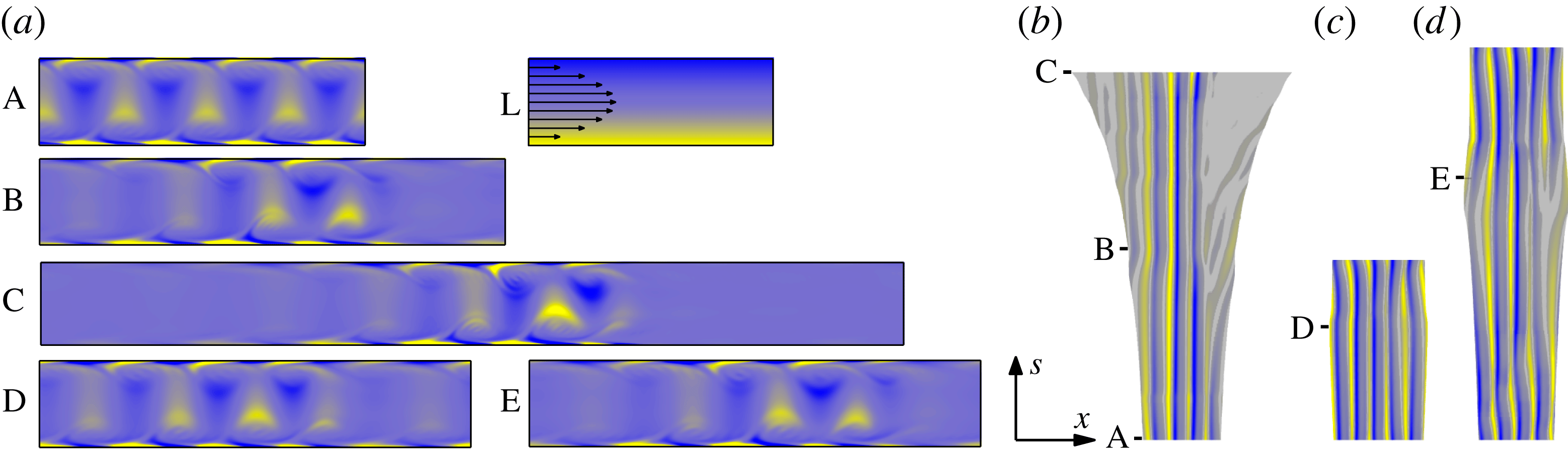
(a) Isovorticity contours of laminar flow (L), Tollmien–Schlichting waves TSWs (A) and modulated Tollmien–Schlicting waves MTSWs for different values of the wavenumber ( $k$ ) and Reynolds number ( $Re$ ) parameters $k$ and $\mathit{Re}$ (B–E). Only perturbation on the laminar flow is represented except for L. Space–arclength parameter ( $\text{d}s\equiv \sqrt{\text{d}\Vert a\Vert ^{2}+(\text{d}k)^{2}}$ , where $a$ is the state vector defining the solution) diagram showing the evolution along (b) an MTSW branch taking $R_{5}$ upper branch (UB) TSWs to localisation at $\mathit{Re}=2800$ , (c) an $R_{5}$ – $R_{5}$ branch at $\mathit{Re}=2800$ and (d) a branch connecting $R_{4}$ UB and $R_{5}$ lower branch (LB) TSWs at $\mathit{Re}=3000$ . The colouring represents the spanwise vorticity along a straight line at $y=-0.9$ and at the time set by the crossing of the Poincaré section used in the solver.

We adopt the streamfunction formulation of Drissi et al. (Reference Drissi, Net and Mercader1999), which naturally satisfies mass conservation and the no-slip boundary condition at the walls, and at the same time preserves a constant mass flow. The non-dimensional streamfunction ${\it\Psi}(x,y;t)$ is related to the non-dimensional velocity field through $u=\partial _{y}{\it\Psi}$ and $v=-\partial _{x}{\it\Psi}$ . The Navier–Stokes equations transform into

with streamwise-periodic boundary conditions and $\partial _{y}{\it\Psi}(x,\pm 1;t)=\partial _{x}{\it\Psi}(x,\pm 1;t)=0$ . The additional condition ${\it\Psi}(x,1;t)-{\it\Psi}(x,-1;t)=4/3$ enforces the constant non-dimensional mean axial velocity of $2/3$ , while ${\it\Psi}(x,-1;t)=-2/3$ is chosen arbitrarily. The basic laminar flow reads ${\it\Psi}_{0}(y)=y(1-y^{2}/3)$ . In what follows, we consider the effect of finite perturbations $\widetilde{{\it\Psi}}(x,y;t)$ to the basic solution,

where $\widetilde{{\it\Psi}}$ is streamwise periodic and verifies homogeneous Neumann–Dirichlet boundary conditions at the walls: $\widetilde{{\it\Psi}}(x,\pm 1;t)=\partial _{x}\widetilde{{\it\Psi}}(x,\pm 1;t)=\partial _{y}\widetilde{{\it\Psi}}(x,\pm 1;t)=0$ . Substituting (2.3) into (2.2) yields an equation for $\widetilde{{\it\Psi}}$ :

with linear and nonlinear operators

3. Numerical approach

We use a Fourier–Legendre spectral expansion to approximate solutions of (2.4) in a domain ${\it\Omega}=\{(x,y)\in [0,{\it\Lambda}]\times [-1,1]\}$ :

where ${\it\Psi}_{\ell m}(x,y)=\text{e}^{\text{i}\ell kx}{\it\Phi}_{m}(y)$ , $\boldsymbol{a}=\{a_{\ell m}\}$ is the state vector with $a_{-\ell m}=a_{\ell m}^{\ast }$ ( $^{\ast }$ denotes complex conjugation), $k=2{\rm\pi}/{\it\Lambda}$ is the minimum streamwise wavenumber and ${\it\Phi}_{m}(y)=(1-y^{2})^{2}\,\text{L}_{m}(y)$ , with $\text{L}_{m}(y)$ the $m$ th Legendre polynomial. Here, ${\it\Phi}_{m}(\pm 1)={\it\Phi}_{m}^{\prime }(\pm 1)=0$ by construction, so that (3.1) identically satisfies homogeneous Dirichlet–Neumann boundary conditions at the walls.

Introducing the inner Hermitian product of two arbitrary streamwise-periodic fields ${\it\zeta}(x,y)$ and ${\it\eta}(x,y)$ in the domain ${\it\Omega}=[0,{\it\Lambda}]\times [-1,1]$ as

application of the spectral Galerkin scheme to (2.4) using (3.1) yields a system of ordinary differential equations for the expansion coefficients $a_{\ell m}(t)$ :

with

Summation over repeated indices is assumed, and $(p,q)\in [0,L]\times [0,M]$ . The nonlinear term $\mathbb{N}_{pq}(\boldsymbol{a})$ is evaluated pseudospectrally using Orszag’s $3/2$ rule for dealiasing.

System (3.3) is advanced in time using a fourth-order linearly implicit backward differences scheme with fourth-order extrapolation for the nonlinear term,

where the superscript indicates the time instant ( $t_{i}=i{\rm\Delta}t$ , with ${\rm\Delta}t$ the time step). The time integration is started with an explicit fourth-order Runge–Kutta method.

The time step has been held constant at ${\rm\Delta}t=10^{-2}$ . A minimum of $50$ Legendre polynomials and $7\times n$ Fourier modes ( $n$ is the number of Tollmien–Schlichting waves that fit in the domain) in the wall-normal and streamwise spectral expansions respectively have been used throughout, but higher resolutions have been deployed for some extreme values of the parameters to ensure convergence.

Travelling (or drifting) waves are characterised by a clear-cut streamwise wavelength ${\it\lambda}_{0}=2{\rm\pi}/k_{0}$ ( $k_{0}$ is the fundamental wavenumber) and a travelling (phase) speed $c$ . The state vector dependence on time simplifies to $a_{\ell m}(t)=a_{\ell m}^{TW}\text{e}^{-\text{i}\ell k_{0}ct}$ . Formal substitution in (3.3) leads to a nonlinear algebraic system of equations for the unknown speed $c$ and complex state vector $\boldsymbol{a}^{TW}=\{a_{\ell m}^{TW}\}$ :

System (3.6) is completed with an extra condition on the phase of the solution to remove streamwise degeneracy and solved by means of a Newton–Krylov method (Kelley Reference Kelley1995), and solution branches are tracked in the $(Re,k_{0})$ parameter space using pseudoarclength continuation (Kuznetsov Reference Kuznetsov2004).

When considered in a periodic domain of their wavelength, upper-branch travelling waves typically undergo a series of superharmonic bifurcations into increasingly complex flows. When considered in longer domains, though, travelling wavetrains may exhibit subharmonic instability.

Here, we will be concerned with subharmonic instability of travelling waves, i.e. instability to infinitesimal perturbations of wavelengths ${\it\lambda}=2{\rm\pi}/k$ (wavenumber $k$ ) longer than that of the wave. Perturbations of this type introduce a streamwise modulation to the wavetrain that may develop into localisation. In principle, $k$ can take any positive real value in the interval $[0,1]$ . For $k/k_{0}=m/n\in \mathbb{Q}$ ( $n\in \mathbb{N}$ , $m=1,\ldots ,n$ ), the instability of a travelling wave of wavenumber $k_{0}$ can be understood as the superharmonic instability of $n$ replicas of the travelling wave filling a periodic domain of length ${\it\Lambda}=n{\it\lambda}_{0}$ to periodic perturbations that fit $m$ times into the domain (Prat, Mercader & Knobloch Reference Prat, Mercader and Knobloch1998; Melnikov et al. Reference Melnikov, Kreilos and Eckhardt2014). Floquet theory analysis shows that modes with $m=j$ and $m=n-j$ are related by conjugation, so that only half of the possible wavelengths need be explored. Furthermore, an analysis for a given $k/k_{0}$ can be performed on the minimal domain $nk_{0}$ , such that $n/m$ expresses an irreducible fraction. Instability to irrational $k/k_{0}$ can only be interpreted in an infinitely long domain.

The representation of $a_{\ell ^{\prime }m}^{TW}$ in the $n$ -fold replicated domain ${\it\Omega}_{n}=[-1,1]\times [0,n{\it\lambda}_{0}],n\in \mathbb{N}$ is

where $k_{n}=k_{0}/n$ and $a_{\ell m}^{TW_{n}}=a_{\ell ^{\prime }m}^{TW}$ for $\ell =n\ell ^{\prime }$ and $0$ otherwise. Linear stability is then analysed by considering infinitesimal disturbances to the travelling wave:

Substituting (3.8) into (3.3) and neglecting terms beyond linear results in the generalised eigenproblem

which can be solved for eigenvalues ${\it\sigma}_{i}$ and eigenvectors ${\bf\epsilon}_{i}=\{{\it\varepsilon}_{\ell m_{i}}\}$ . Here, $D_{\boldsymbol{a}}\mathbb{N}_{pq}^{\ell m}(\boldsymbol{a}^{TW_{n}})$ is the linearisation of $\mathbb{N}$ about $\boldsymbol{a}^{TW_{n}}$ and $(p,q)=[0,nL]\times [0,M]$ . For small $n$ , (3.9) can be solved using direct eigenvalue methods such as QZ (the generalised Schur decomposition). For large resolutions, Arnoldi iteration is required in combination with adequate Cayley transformations (Trefethen & Bau Reference Trefethen and Bau1997).

A comprehensive analysis would incur unaffordable computational time scales, so that the focus has been mainly set on the subset of $k$ values that can be analysed in domains of up to $6{\it\lambda}_{0}$ , which are sufficiently long to initiate a streamwise modulation that effectively localises when followed to longer domains. As a matter of fact, previous subharmonic stability analyses of travelling waves in PPF (Drissi et al. Reference Drissi, Net and Mercader1999) reveal oscillatory Hopf bifurcations from which emanate branches of streamwise-modulated wavetrains (Jimenez Reference Jimenez1990) that are time-periodic when observed from a reference frame moving at the average streamwise speed of the waves.

To compute and track modulated waves beyond their region of stability, we have applied Newton–Krylov and pseudoarclength continuation to the nonlinear system of equations resulting from root finding for the map defined by consecutive crossings of a Poincaré section $\mathbb{P}$ :

where ${\it\Phi}^{t}$ is the flow generated by (3.3) and $\left[\mathbb{T}({\rm\Delta}z)\boldsymbol{a}\right]_{\ell m}=\text{exp}(-\text{i}\ell k{\rm\Delta}z)a_{\ell m}$ is the shift operator. Here, $T$ (the modulation period) and ${\rm\Delta}z$ (the streamwise drift) satisfy

where $[\hat{\mathbb{T}}(\boldsymbol{a})]_{\ell m}=-\text{i}\ell ka_{\ell m}$ is the group orbit tangent and $\dot{\boldsymbol{a}}=\mathbb{A}^{-1}\left[\mathbb{B}\boldsymbol{a}+\mathbb{N}(\boldsymbol{a})\right]$ is the rate of change of the state vector. The orthogonality conditions (3.11) simultaneously define the Poincaré section and remove the drift degeneracy along the group orbit.

4. Results and discussion

Although linearly stable for Reynolds numbers up to $\mathit{Re}_{c}=5772.22$ (Orszag Reference Orszag1971), the basic flow is subcritically unstable to well-known streamwise-periodic drifting waves that go by the name of Tollmien–Schlichting waves (TSW, figure 1 aA; an online supplementary movie is available at http://dx.doi.org/10.1017/jfm.2015.440). The critical wavenumber is $k_{c}=1.02056$ .

Figure 2.

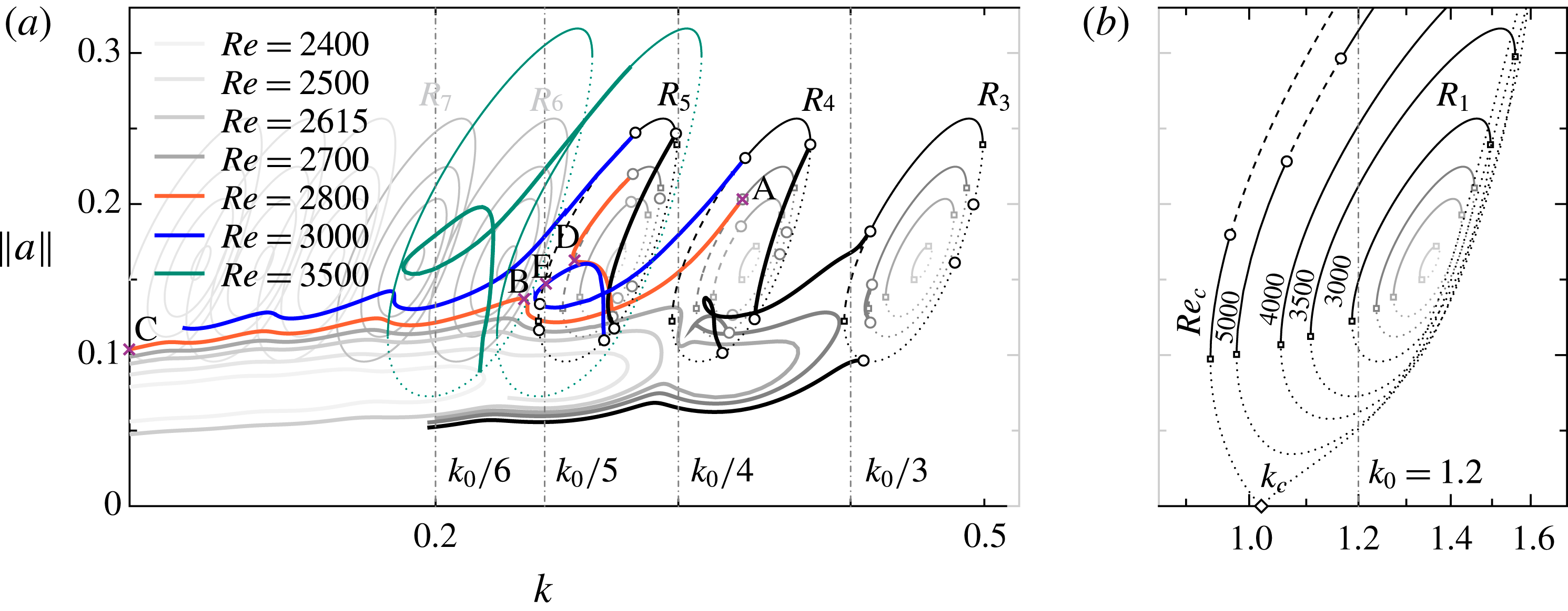
Amplitude of TSWs and MTSWs as a function of $k$ . The number of Fourier modes was adapted during $k$ -continuation to ensure sufficient streamwise resolution. The Reynolds number is colour coded. Thick lines represent MTSWs. Continuous, dashed and dotted thin lines labelled $R_{n}$ denote subharmonically stable UB, unstable UB and LB trains of $n$ TSW solutions. Open squares are saddle–node and open circles Hopf bifurcation points. The diamond indicates the subcritical bifurcation of TSWs from the base flow.

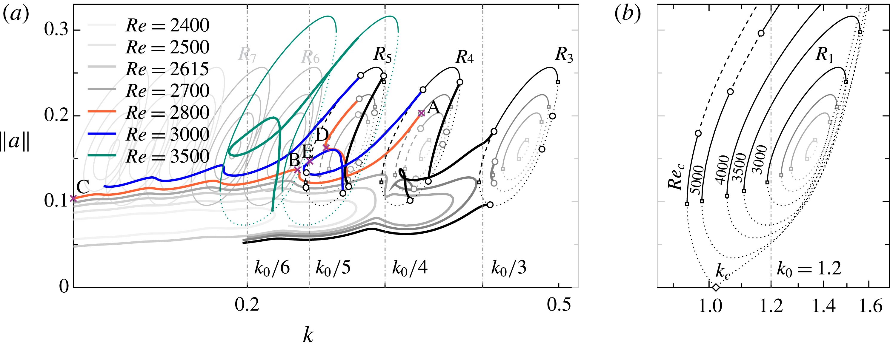
When considered at constant $\mathit{Re}<\mathit{Re}_{c}$ (figure 2, $R_{1}$ ), TSWs appear as disconnected closed loops with a limited range of existence $k_{0}\in [k_{0_{min}}(\mathit{Re}),k_{0_{max}}(\mathit{Re})]$ , such that within these limits two solutions exist for any given $k$ that may be classified as either upper (UB, continuous and dashed lines) or lower (LB, dotted) branch. We have followed the steps of Pugh & Saffman (Reference Pugh and Saffman1988) and Jimenez (Reference Jimenez1990) in computing the superharmonic stability of TSWs to validate our numerics. Lower-branch TSWs are mere saddles, while upper-branch TSWs, which are initially stable, undergo a series of transitions into increasingly complex flows that result in chaotic dynamics well before $\mathit{Re}_{c}$ is reached (Jimenez Reference Jimenez1990) (see the unstable regions – dashed lines – of $R_{1}$ in figure 2). When considered in longer domains, though, TSW trains exhibit subharmonic instability.

For the subharmonic stability we have systematised the analysis of Drissi et al. (Reference Drissi, Net and Mercader1999) to explore up to $\mathit{Re}=3000$ in domains of length ${\it\Lambda}=(2{\rm\pi}/k_{0})n$ with $n\leqslant 6\in \mathbb{N}$ . Figure 2 represents a normalised measure of the amplitude of the solution ( $\Vert \boldsymbol{a}\Vert =\left[\sum _{\ell m}|a_{\ell m}|^{2}\right]^{1/2}$ ) against the extent of the periodic domain as measured by the smallest wavenumber ( $k=2{\rm\pi}/{\it\Lambda}$ ) it can accommodate. Thus, the TSW family $R_{1}$ appears replicated in figure 2 at $k=k_{0}/n$ for $n\in \mathbb{N}$ , each replica representing a train of $n$ TSWs that fits exactly once into the domain under consideration ( $R_{n}$ TSW solution, standing for $n$ replicas).

At large enough $\mathit{Re}$ and low enough $k$ , the TSW iso- $\mathit{Re}$ curves start to intersect (see the fading $R_{n}$ families in figure 2), indicating that the same periodic domain can take various TSW trains including different numbers of replicas of the appropriate wavelength. The subharmonic bifurcation analysis results in a set of curves in $\mathit{Re}$ – $k$ parameter space that reduce to bifurcation points when considered at constant $\mathit{Re}$ (open circles). These points, together with the saddle–node points, divide each iso- $\mathit{Re}$ loop of TSWs into segments with a different count of unstable eigenmodes. A distinction has been made between the unstable LB (dotted), the stable part of the UB (solid) and, if present, the subharmonically unstable portions of the UB (dashed).

All subharmonic instabilities happen to be of the Hopf type, such that emanating solutions incorporate a modulational frequency in addition to the degenerate frequency associated with the streamwise solid-body motion of the TSW. We have continued the modulated Tollmien–Schlichting waves (MTSWs) to analyse the nonlinear evolution of the streamwise modulation resulting from the subharmonic instability. The family of MTSWs has a convoluted dependence on the parameters that hinders a simple interpretation, which is resolved by analysing one parameter at a time.

Some of the constant- $\mathit{Re}$ branches go from a train of a certain number $n$ of TSWs to another train with the same number of TSWs with an interim of a mild temporal modulation that introduces a group velocity on top of the phase velocity of the TSW. Figure 1(c) recreates one such continuation, for an $\mathit{Re}=2800$ branch of MTSWs connecting with $R_{5}$ at both ends (short orange line in figure 2), by picturing the evolution of vorticity on a streamwise section at $y=-0.9$ as progress is made along the continuation curve. The maximum departure from steadiness is labelled D and vorticity contours are shown in figure 1(a)D.

Other branches evolve into localisation. Figure 1(b) shows the branch issued, also at $\mathit{Re}=2800$ , from the instability of a slightly longer TSW (figure 1 aA) to perturbations of a shorter wavelength that modulates trains of four replicas ( $R_{4}$ ). The localised solution of figure 1(a)C (online movie) shares key features with puffs and spots in other shear flows: while the leading edge modifies the laminar flow in the midplane, the trailing edge has a tendency to attach to the walls. The process that leads to the localised solution is nevertheless non-monotonic, as weak TSWs try to grow within the quasilaminar space left in between separating replicas. Traces of these weak TSWs appear as fading coloured bands in figure 1(b) and are manifested in figure 2 (long orange line) as failed attempts of the branch to loop back to reconnect with a longer train of TSWs. The first attempt at reconnection is labelled B and shown in figure 1(a)B (online movie). The MTSWs labelled B and D in figure 1 correspond to turns of the continuation branches facing each other in figure 2 (orange lines). The snapshots, shown in figure 1(a), indeed bear some resemblance to one another, which indicates proximity. As a matter of fact, the two branches approach at these points as $\mathit{Re}$ is increased, collide and separate into two new branches at $\mathit{Re}=3000$ , one that localises from $R_{5}$ and another that connects $R_{4}$ to $R_{5}$ (blue lines). This latter branch shows a tendency to localise, as evidenced in figure 1(d) by the widening grey region half-way along the continuation, but rectifies in a loop to end up incorporating a new replica of TSWs. The snapshot labelled E and depicted in figure 1(a)E is in fact related to B and D through a codimension-two bifurcation point somewhere around $(k,\mathit{Re})\sim (0.3,2900)$ . This trend is corroborated at $\mathit{Re}=3500$ (green lines), where the branch localising from $R_{5}$ at $\mathit{Re}=3000$ has already evolved into a loop connecting $R_{5}$ to $R_{6}$ .

It might be argued that, unlike the localised MTSWs studied here, streamwise-localised solutions in other shear flows are not patterned (Duguet et al. Reference Duguet, Schlatter and Henningson2009; Mellibovsky et al. Reference Mellibovsky, Meseguer, Schneider and Eckhardt2009), so that the localisation mechanism might be fundamentally different from the one we describe. However, there is evidence that pipe Poiseuille localised solutions (Avila et al. Reference Avila, Mellibovsky, Roland and Hof2013; Chantry et al. Reference Chantry, Willis and Kerswell2014) are indeed patterned, except that the wavy structure is in fact masked by the rather short modulational envelope. Chaotic sets developed from extended versions of these solutions clearly exhibit wavetrains with a varying count of wave periods embedded (authors’ unpublished observations). This will most probably be the case for localised plane Couette and plane Poiseuille solutions too (Brand & Gibson Reference Brand and Gibson2014; Zammert & Eckhardt Reference Zammert and Eckhardt2014). The non-snaking localisation mechanism (Burke & Knobloch Reference Burke and Knobloch2006) found in double-diffusive convection (Beaume, Knobloch & Bergeon Reference Beaume, Knobloch and Bergeon2013b ) cannot apply to plane Couette, plane Poiseuille or pipe flows, as the required condition that a non-trivial streamwise-independent state exists is not fulfilled by any of these flows.

Figure 3.

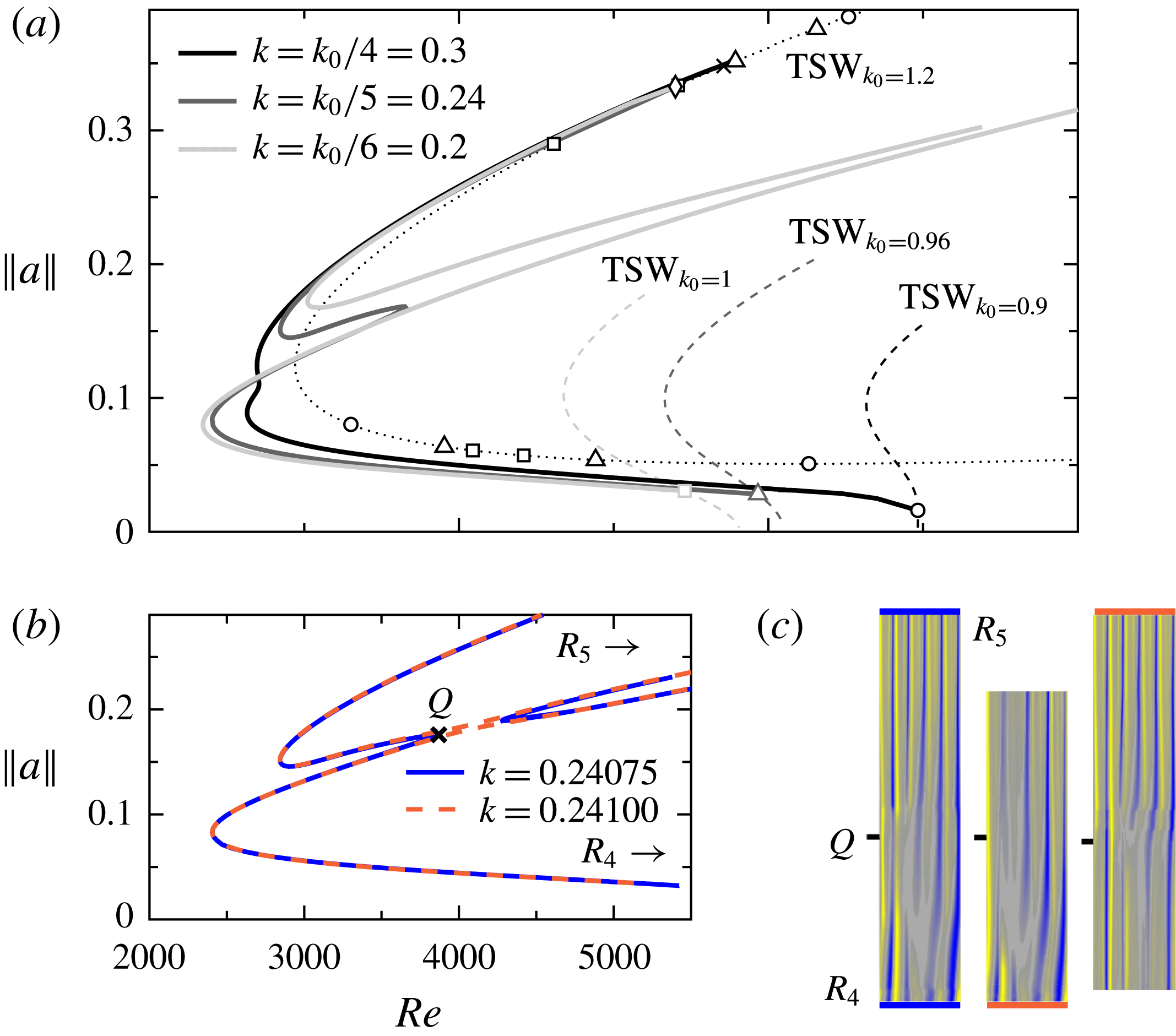
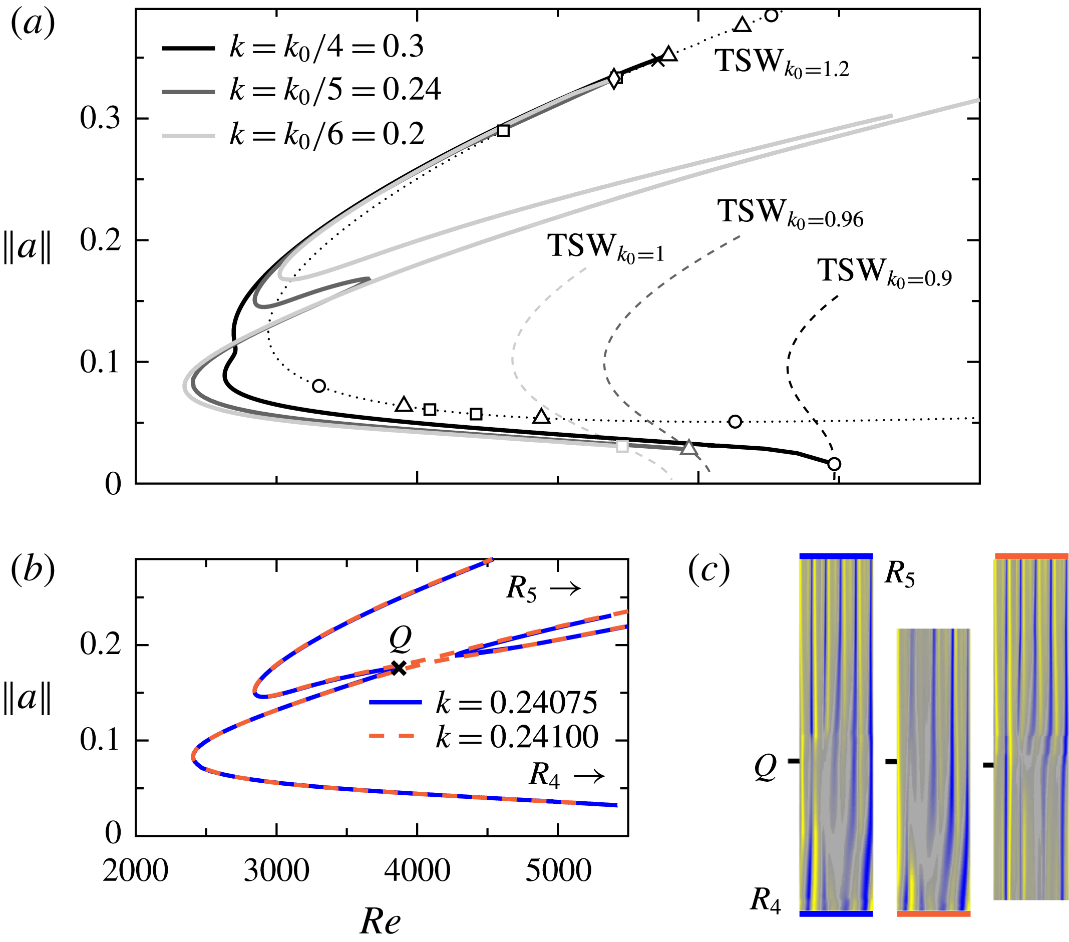
(a) The $\mathit{Re}$ -continuation of MTSWs (solid lines; at $k$ values as indicated in figure 2) compatible with subharmonic modulation of the $k=1.2$ TSW (dotted) and their connections with LB TSWs. The circles, triangles, squares and diamonds represent $n=3$ – $6$ subharmonic Hopf bifurcations respectively. Irrelevant MTSWs have not been plotted for clarity. The cross marks the first superharmonic Hopf bifurcations. The scale and labels for the $x$ -axis are shared with those of (b). (b) The MTSWs at neighbouring values of $k$ and (c) corresponding space–arclength diagrams. Here, $R_{4}$ and $R_{5}$ denote connections to TSWs, while $Q$ indicates solutions closely related by a codimension-2 point.

It is clear from $k$ -continuation that MTSWs connect with both upper- and lower-branch TSWs, and how this comes about when smoothly varying $\mathit{Re}$ at constant $k$ is vital to putting the snaking hypothesis to test. The simplest approach to the issue is to select a TSW with fixed $k_{0}$ as a reference and restrict the $\mathit{Re}$ -continuation of MTSW branches to domains with $k=k_{0}/n,n\in 3,4,5,6\ldots .$ We have chosen $k_{0}=1.2$ to have some of the continuation branches cut right through the loops (see figure 2). Figure 3(a) shows $\mathit{Re}$ -continuation branches for $k=k_{0}/4$ , $k_{0}/5$ and $k_{0}/6$ . The $k=k_{0}/4$ branch (continuous black line) connects seemingly uneventfully an LB $R_{3}$ with a UB $R_{4}$ . The $k_{0}/5$ branch (dark grey), which cuts right through a $k$ -continuation loop, seems to hint at a snaking-like process by incorporating a back-and-forth detour in the otherwise uneventful connection of an LB $R_{4}$ and a UB $R_{5}$ . The $k_{0}/6$ branch (light grey), however, while still connecting with an LB $R_{5}$ , challenges the pattern by neither connecting with a UB nor even hinting at an approach to connect at higher  $\mathit{Re}$ .

Although for some particular moderate values of $k$ , $\mathit{Re}$ -continued branches of MTSWs bend back and forth in a snaking-like fashion connecting different trains of TSWs that fit in the same domain, the accumulation process that is typical of spanwise localisation is not robust. Figure 3(b,c) shows how small variations in $k$ disrupt the continuous single branch (continuous blue line), which breaks into two separate branches (dashed orange) that reach high $\mathit{Re}$ values, possibly infinity. While both continuations evolve parallely away from LB $R_{4}$ TSWs, one manages to incorporate a new replica ( $k=0.24075$ ) and connect to $R_{5}$ , while the other keeps the modulation and a certain localisation for increasing $\mathit{Re}$ ( $k=0.24100$ ). For large enough domains, it appears utterly improbable that a localised MTSW will robustly accumulate the number of bends that are required before connection to a full train of UB TSWs is effective. Instead, most, if not all, of the bends will have broken up producing disconnected families of localised MTSWs of different lengths. The $k=0.2$ upper lobe in figure 3(a) (light grey) is a clear example of how disconnected families of solutions with different modulated wavenumber counts can arise in the same domain. In longer domains this will result in disconnected localised solutions of different lengths. Even when one of these bends exists, there also exists a disconnected branch of MTSWs that appears in a saddle–node at a higher $\mathit{Re}$ and faces the saddle–node of the bend. It is precisely the collision of these two saddle–nodes upon smoothly varying $k$ that disrupts the snaking mechanism. This is reminiscent of the blending of separate regions of regular and semi-infinite snaking into a unique region of semi-infinite snaking observed for some parameter values of the Swift–Hohenberg equation (Burke & Knobloch Reference Burke and Knobloch2006). Furthermore, the existence of a conserved quantity, which in our case is mass flux, accounts for the slanted arrangement of the leftmost saddle–nodes (Dawes Reference Dawes2008; Beaume et al. Reference Beaume, Bergeon, Kao and Knobloch2013a ), thus allowing for localised solutions to exist at lower and higher values of the parameter than are possible in regular snaking. Physically, this means that while the multiplicity of spanwise-localised solutions of different lengths is restricted to a finite $\mathit{Re}$ range (where the bends exist, within the broadened Maxwell point), a surging number of streamwise-localised solutions of varying length extending to high $\mathit{Re}$ appears as longer domains are considered.

Figure 4.

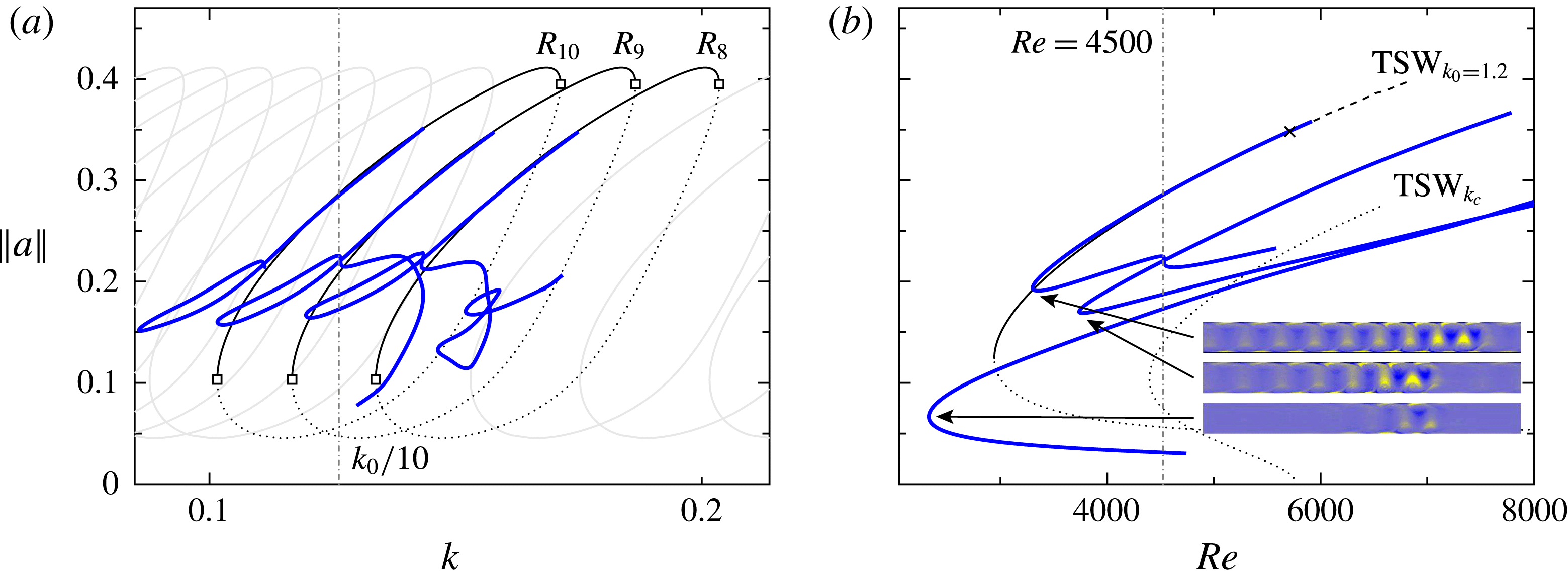
(a) The $k$ -continuation of MTSWs at $\mathit{Re}=4500$ issued from subharmonic instability of $R_{8}$ – $R_{10}$ TSWs. (b) The $\mathit{Re}$ -continuation of MTSWs at $k=k_{0}/10=0.12$ . The cross marks the first superharmonic Hopf bifurcation. The snapshots correspond to the saddle–nodes of the three disconnected branches of MTSWs. The dash-dotted lines in (a) and (b) indicate the cross-sections depicted in (b) and (a) respectively.

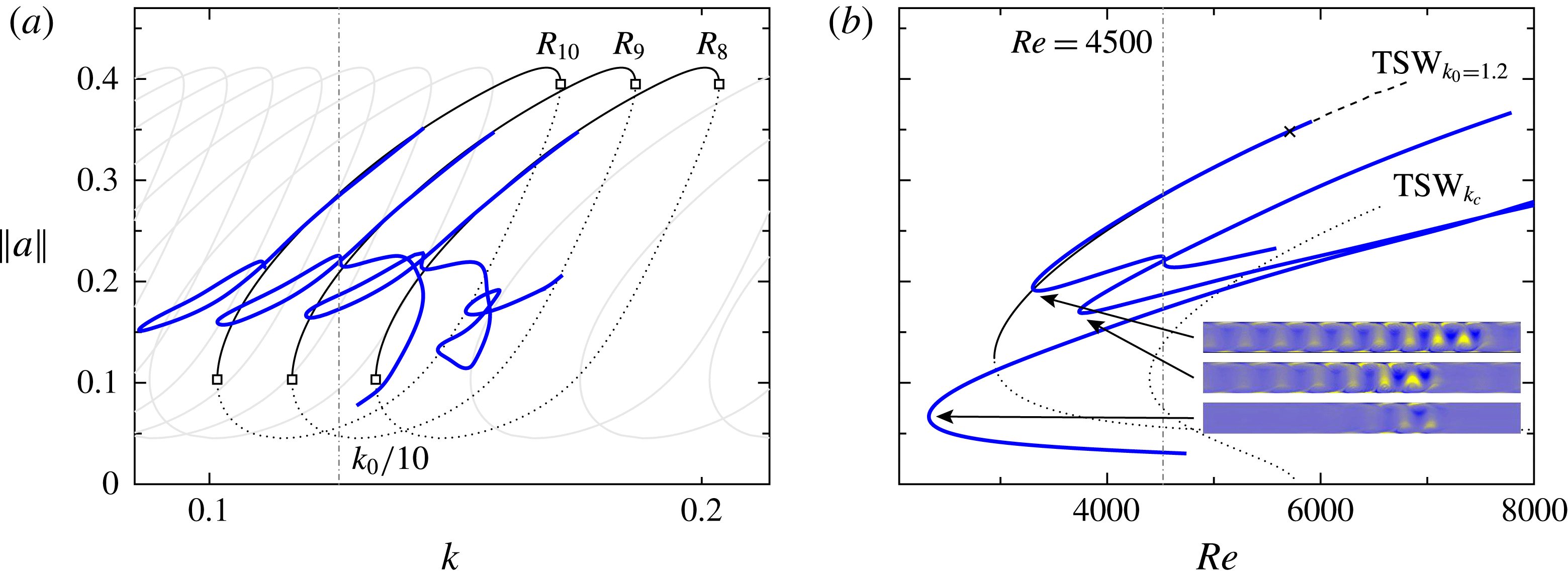
Figure 4(a) illustrates the accumulation process of loops at $\mathit{Re}=4500$ and $k$ around 1.2 ( $R_{10}$ ). The leftmost loop in figure 2 (green line) at $\mathit{Re}=3500$ has stretched and, as TSWs get cluttered in longer domains at higher $\mathit{Re}$ , continuation loops of MTSWs start overlapping in $k$ . Each loop implies a disconnection of MTSW branches when continued in $\mathit{Re}$ , such that three lobes are expected for $k=k_{0}/10=0.12$ in figure 4(b). As a matter of fact, the domain size chosen cuts right through the rightmost end of the loop, which indicates that the upper lobe is just forming. For $k$ slightly lower, the three lobes are perfectly established. This completes the picture of the intricate accumulation process. As the domain size is increased, an upper branch forms from a longer train of shorter TSWs that combines with the uppermost existing lobe as the rightmost part of the iso- $\mathit{Re}$ loop is encountered. Meanwhile, the pre-existing lobes get compressed and the lowest two connect and merge as the leftmost side of the loop is crossed (as shown in figure 3 b). All in all, as loops accumulate, the creation of new lobes at the top is faster than the merging of lobes at the bottom and an increasing number of disconnected branches coexist as longer domains are considered. The snapshots in figure 4 correspond to the saddle–nodes of the various lobes. It is clear that longer localised MTSWs, embedding a higher count of TSW replicas, are encountered as higher lobes are considered. All of these solutions coexist beyond large enough $\mathit{Re}$ in sufficiently long domains.

Symmetries and the nature of the existing non-trivial extended solutions play a key role in homoclinic snaking. Regular snaking results from stationary front pinning to the wavetrain underlying the localised solution (Burke & Knobloch Reference Burke and Knobloch2006). Homogeneous extended solutions give rise to non-snaking behaviour as the fronts can pin to the underlying solution regardless of its spatial extent, but only so for values of the governing parameter corresponding to Maxwell points (Burke & Knobloch Reference Burke and Knobloch2006; Beaume et al. Reference Beaume, Knobloch and Bergeon2013b ). No such behaviour can be expected in the streamwise direction of any of the usual shear flows, as all secondary solutions are patterned. Regarding symmetries, the absence of space reversibility due to the fore–aft broken symmetry of Poiseuille flow introduces significant modifications to the snaking scenario, as demonstrated for simple models such as the Swift–Hohenberg equation (Burke, Houghton & Knobloch Reference Burke, Houghton and Knobloch2009). Among the predicted changes, we have observed the obvious drift of the localised solutions, but no such thing as the disconnection of snakes and ladders into isolas has been detected. Although snaking was originally discovered and studied in variational systems, it is a well-known fact that the problem needs not be variational in time to produce this type of behaviour, as demonstrated for dissipative systems such as plane Couette flow (Schneider et al. Reference Schneider, Gibson and Burke2010). Finally, the introduction of a large-scale neutral mode (Dawes Reference Dawes2008), associated with the existence of a conservation law, results in a substantial enlargement of the region of existence of localised states, and the snaking branches become slanted. Two-dimensional PPF conserves mass flux (or, alternatively, the mean pressure gradient), which justifies the slanted arrangement of the leftmost saddle–nodes even if snaking has been disrupted and isolated branches of localised solutions have emerged.

5. Concluding remarks

We have adopted a streamfunction formulation for two-dimensional flows and introduced a set of purposely developed numerical methods to solve and track in parameter space both travelling and modulated travelling wave solutions, as well as to compute their linear stability.

We have used these methods to dissect the mechanism for shear flow streamwise localisation through its analysis in the paradigmatic case of two-dimensional PPF in order to unveil its resemblance yet at the same time essential differences with spanwise localisation. While its emergence follows subharmonic instability of a periodic wave, the snaking mechanism whereby a long spatial modulation develops into a localising envelope that confines a shrinking wavepacket via the successive loss of wave replicas decisively breaks down. As a result, while the multiplicity of spanwise-localised solutions of different lengths is restricted to a limited $\mathit{Re}$ range, in very long domains branches of arbitrarily long streamwise-localised solutions – their length necessarily quantised – extend to high $\mathit{Re}$ , thus potentially contributing to the formation and growth of a chaotic saddle that may sustain turbulent transients. We have found evidence, in a much longer domain with $k=0.08$ , of phenomena such as quasiperiodicity and chaos, a precursor to turbulence, as well as splitting of localised spots. A thorough analysis of the mechanisms behind these observations is underway but beyond the scope of the present study.

In simple models featuring snaking, localised solutions can be understood as homoclinic orbits of the spatial ordinary differential equation that results from dropping the time derivative (Kirchgässner Reference Kirchgässner1982; Budd & Kuske Reference Budd and Kuske2005). These homoclinic orbits go from the base flow (a spatial fixed point) back to the base flow, with a natural number of intervening quasiorbits around the non-trivial patterned flow (a spatial periodic orbit), hence the qualifier homoclinic with which the word snaking is commonly prefixed. In the limit, a front can be interpreted as a heteroclinic orbit joining the base state and the patterned state. This simple interpretation does not apply to localised solutions in shear flows such as plane Poiseuille or pipe Poiseuille (at least not straightforwardly), as the modulational nature of solutions precludes stationary front pinning, such that time dependence cannot be eliminated from the partial differential equation. Recent studies in our same set-up of two-dimensional PPF suggest that at high Reynolds numbers where turbulence expands, the analysis of laminar–turbulent interfaces may require a specific treatment (Teramura & Toh Reference Teramura and Toh2015).