2 Direct numerical simulation

A DNS has been performed to study the flow around a rectangular cylinder. To the best of the authors’ knowledge, this is the first DNS performed in such a canonical flow for a sufficiently high Reynolds number. Indeed, several numerical studies have been performed in the past, most of them making use of modelling approaches, see Bruno et al. (Reference Bruno, Salvetti and Ricciardelli2014) for a detailed review of simulations (and also experiments) performed in such a flow configuration. The only attempt to face the problem via DNS has been that of Hourigan et al. (Reference Hourigan, Thompson and Tan2001), but the analysis has been carried out for very low Reynolds numbers, namely $Re=350$ , 400 and 500, and a fully developed turbulent state has not been achieved.

The evolution of the flow is governed by the continuity and momentum equations,

(2.1) $$\begin{eqnarray}\displaystyle \left.\begin{array}{@{}c@{}}{\displaystyle \frac{\unicode[STIX]{x2202}u_{i}}{\unicode[STIX]{x2202}x_{i}}}=0\\ {\displaystyle \frac{\unicode[STIX]{x2202}u_{i}}{\unicode[STIX]{x2202}t}}+{\displaystyle \frac{\unicode[STIX]{x2202}u_{i}u_{j}}{\unicode[STIX]{x2202}x_{j}}}=-{\displaystyle \frac{\unicode[STIX]{x2202}p}{\unicode[STIX]{x2202}x_{i}}}+{\displaystyle \frac{1}{Re}}{\displaystyle \frac{\unicode[STIX]{x2202}^{2}u_{i}}{\unicode[STIX]{x2202}x_{j}x_{j}}},\end{array}\right\} & & \displaystyle\end{eqnarray}$$

where $x=x_{1}$ ( $u=u_{1}$ ), $y=x_{2}$ ( $v=u_{2}$ ), $z=x_{3}$ ( $w=u_{3}$ ) are the streamwise, vertical and spanwise directions (velocities), $p$ is the pressure field and $Re=U_{\infty }D/\unicode[STIX]{x1D708}$ is the Reynolds number with $\unicode[STIX]{x1D708}$ the kinematic viscosity, $U_{\infty }$ the free stream velocity and $D$ the thickness of the plate. The OpenFOAM^® finite volume open source code (Weller, Tabor, Jasak & Fureby Reference Weller, Tabor, Jasak and Fureby1998) was used to numerically solve the Navier–Stokes equations (2.1). In particular, equations (2.1) are discretized by means of a structured Cartesian grid of hexahedral cells. The numerical technique is based on central spatial interpolation operators of the second order whereas time integration is performed with a second-order backward Euler implicit scheme. The pressure–velocity coupling is performed with the pressure-implicit split-operator algorithm (Issa Reference Issa1986). Inlet–outlet boundary conditions are imposed in the streamwise direction. The inlet condition is the free stream velocity $U_{\infty }$ . The outlet boundary condition combines a Neumann/Dirichlet condition. In particular, it imposes a zero gradient when the flow is pointing outward at the boundary whereas it imposes a zero velocity when an inward flow is detected. The same boundary condition is imposed in the vertical direction, the only difference being that in the case of inward flow, the imposed condition on velocity is $U_{\infty }$ for the streamwise component and zero for the other two components. Finally, periodic boundary conditions are imposed in the spanwise direction.

Figure 1.

Configuration of the system.

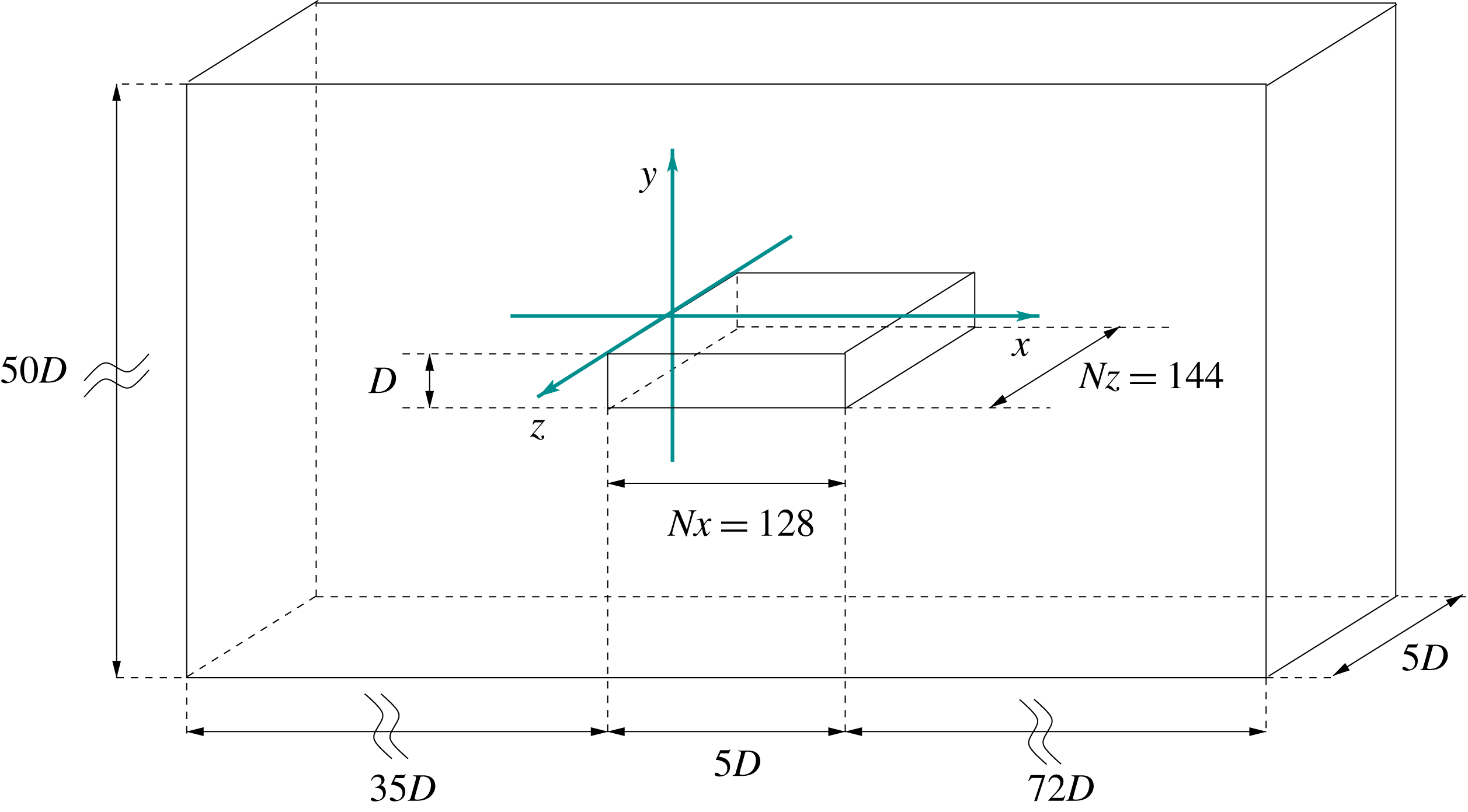
The flow case consists of a rectangular plate whose lengths are $(L_{x},L_{y})=(5D,D)$ , see figure 1. The considered Reynolds number is $Re=3000$ . The extent of the numerical domain is $({\mathcal{D}}_{x},{\mathcal{D}}_{y},{\mathcal{D}}_{z})=(112D,50D,5D)$ and, through the a posteriori analysis of two-point spatial correlation functions, is found to be large enough to not interfere with the flow dynamics. The structured Cartesian grid employed is composed by $1.5\times 10^{7}$ volumes. In particular, the number of volumes above the rectangular plate is $(Nx,Nz)=(128,144)$ . The volume distribution is homogeneous in the spanwise direction while in the streamwise and vertical directions a geometric progression is adopted, $\unicode[STIX]{x0394}x_{i}=k_{x}^{i-1}\unicode[STIX]{x0394}x_{1}$ and $\unicode[STIX]{x0394}y_{j}=k_{y}^{j-1}\unicode[STIX]{x0394}y_{1}$ with $k_{x}=1.06$ , $k_{y}=1.04$ , $\unicode[STIX]{x0394}x_{1}=0.004$ and $\unicode[STIX]{x0394}y_{1}=0.004$ . This approach is used to obtain higher resolution levels in the near-wall leading- and trailing-edge regions. Three main grid resolution issues arise and are given by the discretization of the sharp corners, of the boundary layer regions and of the turbulent core regions. Concerning the sharp corners, the size of the surrounding cells is $(\unicode[STIX]{x0394}x,\unicode[STIX]{x0394}y,\unicode[STIX]{x0394}z)=(0.004,0.004,0.0347)$ and is also found to be sufficiently small when compared with other approaches such as those collected in Bruno et al. (Reference Bruno, Salvetti and Ricciardelli2014). Concerning the near-wall resolution, the boundary layers are characterized by small levels of turbulence owing to their very short development length. Hence, the more important near-wall resolution requirement is given by the correct discretization of the vertical gradients rather than of the turbulence. In terms of friction units, the mean grid resolution employed is $(\overline{\unicode[STIX]{x0394}x^{+}},\overline{\unicode[STIX]{x0394}y^{+}},\overline{\unicode[STIX]{x0394}z^{+}})=(6.1,0.31,5.41)$ where $\overline{(\cdot )}$ denotes the streamwise average along the rectangle length. Owing to the highly inhomogeneous behaviour of friction which essentially reflects the upstream and downstream accelerations of the boundary layers rather than the development of small-scale fluctuations, the local behaviour of resolution in friction units significantly varies from minima of the order $(\unicode[STIX]{x0394}x_{min}^{+},\unicode[STIX]{x0394}y_{min}^{+},\unicode[STIX]{x0394}z_{min}^{+})=(0.1,0.003,0.6)$ to maxima of the order $(\unicode[STIX]{x0394}x_{max}^{+},\unicode[STIX]{x0394}y_{max}^{+},\unicode[STIX]{x0394}z_{max}^{+})=(34,0.375,30)$ . As a reference, let us note that in the forward boundary layer region, the local behaviour of the present resolution is found to be comparable with that reported by Yao, Thomas, Sandham & Williams (Reference Yao, Thomas, Sandham and Williams2001), where a grid refinement study of the trailing-edge separation of a fully turbulent boundary layer is carried out. As far as the resolution of the turbulent core regions is concerned, this is assessed by using the Kolmogorov scale $\unicode[STIX]{x1D702}=(\unicode[STIX]{x1D708}^{3}/\unicode[STIX]{x1D716})^{(1/4)}$ . We measure $(\unicode[STIX]{x0394}x\unicode[STIX]{x0394}y\unicode[STIX]{x0394}z)^{1/3}/\unicode[STIX]{x1D702}<2.2$ in the leading-edge shear layer where the transitional mechanisms take place, whereas $(\unicode[STIX]{x0394}x\unicode[STIX]{x0394}y\unicode[STIX]{x0394}z)^{1/3}/\unicode[STIX]{x1D702}<6.2$ in the turbulence core region above the plate and $(\unicode[STIX]{x0394}x\unicode[STIX]{x0394}y\unicode[STIX]{x0394}z)^{1/3}/\unicode[STIX]{x1D702}<3.8$ in the wake. Finally, the time step is kept variable throughout the simulation to obtain a condition $\mathit{CFL}<1$ in each point of the domain. The resulting time step, on average, is $\unicode[STIX]{x0394}t=0.0023$ .

In the present flow case, the computational demand for well-converged statistics denoted as $\langle \cdot \rangle$ is mitigated by the statistical stationarity of the flow field and by the statistical homogeneity in the spanwise direction. Furthermore, the flow exhibits certain statistical symmetries in the vertical direction that are better expressed by shifting the origin of the vertical coordinate to the centre of the rectangle, ${\tilde{y}}=y-D/2$ . Indeed, the transformation ${\tilde{y}}\rightarrow -{\tilde{y}}$ leaves quantities such as $U=\langle u\rangle$ and $\langle u_{i}u_{i}\rangle$ statistically invariant while reversing the signs of quantities such as $V=\langle v\rangle$ , $\langle uv\rangle$ and $\unicode[STIX]{x2202}\langle \cdot \rangle /\unicode[STIX]{x2202}{\tilde{y}}$ . Accordingly, the average of a generic quantity $\unicode[STIX]{x1D6FD}$ is defined as

(2.2) $$\begin{eqnarray}\langle \unicode[STIX]{x1D6FD}\rangle (x,{\tilde{y}})=\frac{1}{N}\mathop{\sum }_{i=1}^{N}\frac{1}{2}\left(\frac{1}{L_{z}}\int _{-L_{z}/2}^{L_{z}/2}\unicode[STIX]{x1D6FD}(x,+{\tilde{y}},z,t)\,\text{d}z\pm \frac{1}{L_{z}}\int _{-L_{z}/2}^{L_{z}/2}\unicode[STIX]{x1D6FD}(x,-{\tilde{y}},z,t)\,\text{d}z\right)\!,\end{eqnarray}$$

where the sum and difference of the two integrals are imposed by the symmetric/antisymmetric nature of the considered variable. After reaching a statistical steady state, the fields are collected at a number $N=317$ of samples separated in time by $\unicode[STIX]{x0394}T=T$ where $T=D/U_{\infty }$ is the characteristic time scale of the flow. In the following, the customary Reynolds decomposition of the flow in a mean and fluctuating field is adopted, i.e.  $u_{i}=U_{i}+u_{i}^{\prime }$ and $p=P+p^{\prime }$ . If not stated specifically, variables are hereafter presented as dimensionless by using $D$ for lengths and $D/U_{\infty }$ for times.

3 Mean flow features

Figure 2.

(a) Streamlines of the mean velocity field $(U,V)(x,y)$ . The primary vortex, secondary vortex and wake vortex, denoted as PV, SV and WV, are identified with green, red and cyan streamlines, respectively. The shaded regions show the mean shear for values $|\unicode[STIX]{x2202}U/\unicode[STIX]{x2202}y|>4$ . The relevant locations P1, P2, P3, P4 and P5 used for the analysis of the spatial correlations § 5 and of the temporal signals § 7, are also reported. (b) Isocontours of the mean pressure field $P(x,y)$ . (c) Isocontours of turbulent kinetic energy $\langle q\rangle =\langle u_{i}^{\prime }u_{i}^{\prime }\rangle /2$ . In (b) and (c) the dashed lines report the location of the primary vortex, secondary vortex and wake vortex.

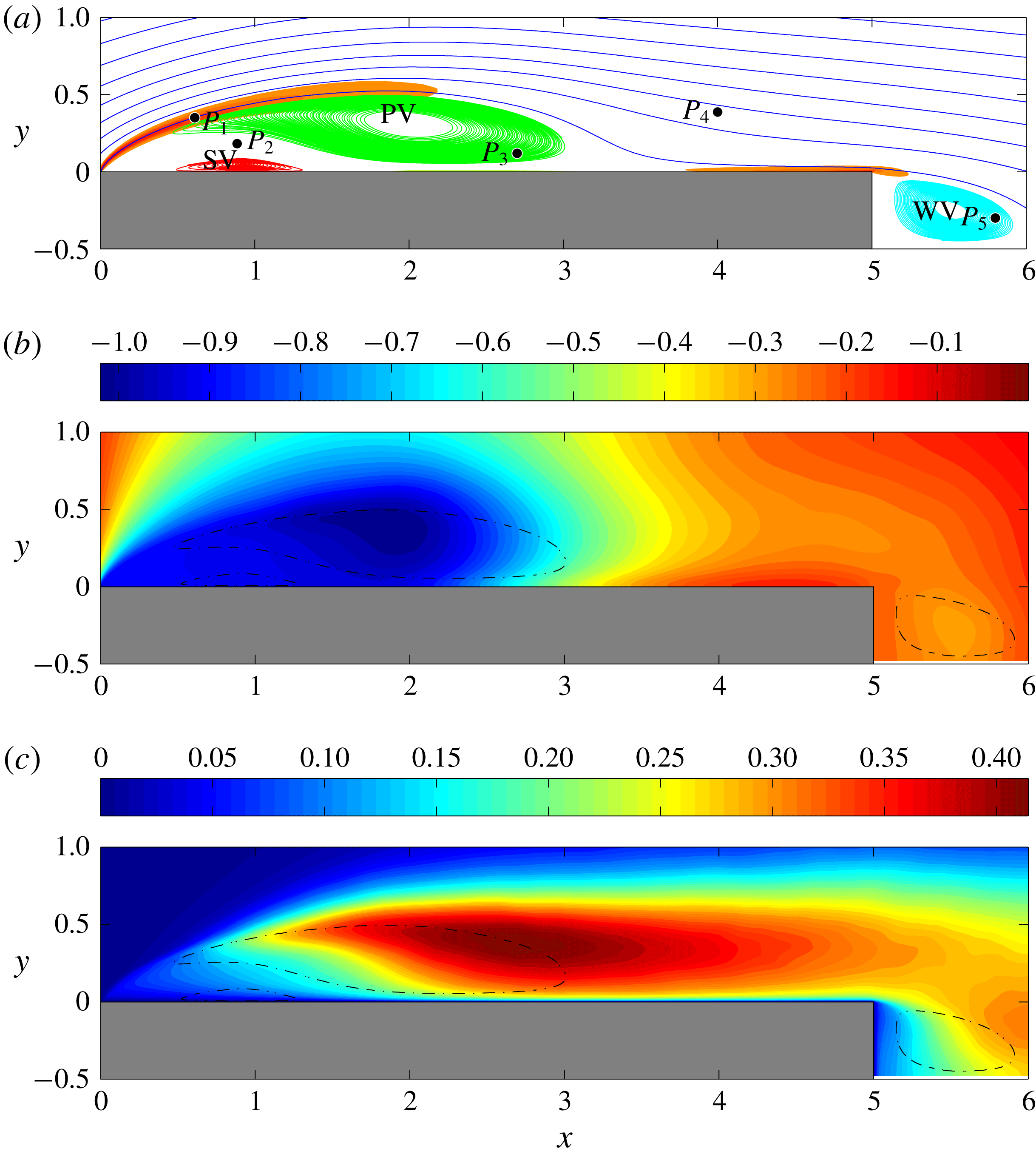
In this section, we report the main features of the mean flow. As shown in figure 2(a), the streamlines of the mean flow highlight the presence of a separation at the leading edge and of a reattachment at $x_{r}\approx 3.65$ . Hence, a large-scale recirculation is present on average and will hereafter be called the primary vortex, see the green lines in figure 2(a). The flow separation gives rise to a strong leading-edge free-shear layer as highlighted in figure 2(a), where the regions of the flow characterized by high levels of mean shear are also shown. In fact, a second recirculating bubble is present and highlighted with red lines again in figure 2(a). This secondary vortex is located below the primary vortex. Indeed, the reverse flow induced in the near-wall region by the primary vortex creates a boundary layer moving upstream. As shown by the isocontours of the mean pressure field in figure 2(b), the induced boundary layer undergoes an adverse pressure gradient, hence it decelerates, becomes thicker and, finally, breaks down leading to separation (Simpson Reference Simpson1989). Hence, the secondary vortex, being induced by the primary vortex, is counter-rotating with respect to the primary vortex and its characteristic length and time scales are smaller than those of the primary vortex. After the average reattachment point for $x>x_{r}$ , the flow evolves in a downstream boundary layer and finally detaches at the trailing edge thus forming a third recirculating region hereafter called wake vortex, see the cyan lines in figure 2(a). Further details can be found in Cimarelli, Leonforte & Angeli (Reference Cimarelli, Leonforte and Angeli2018).

The isocontours of turbulent kinetic energy $\langle q\rangle =\langle u_{i}^{\prime }u_{i}^{\prime }\rangle /2$ shown in figure 2(c) highlight the initial almost laminar state of the leading-edge shear layer. Instabilities associated with the shear-layer amplify the intensity of the fluctuations thus giving rise to turbulence. The maximum intensities of turbulent kinetic energy are reached in a region which elongates itself in the streamwise direction and crosses the external paths of the large scale recirculation. This region will be hereafter called primary vortex shedding region. The peak of the turbulent kinetic energy is located at $(x,y)\approx (2.7,0.4)$ . Then, moving downstream, the turbulent fluctuations decrease their magnitude but retain their local maxima far away from the wall for $y\approx 0.35$ . This behaviour of $\langle q\rangle$ inverts while moving through the wake where turbulent kinetic energy increases again forming a local maximum in a region just behind the wake vortex centered at $(x,y)\approx (6.2,0.15)$ . For further details, see Mollicone et al. (Reference Mollicone, Battista, Gualtieri and Casciola2017) where the energetics of separating and reattaching flows are assessed by analysing the mean and turbulent kinetic energy budgets.

4 Instantaneous flow topology

Figure 3.

Instantaneous flow realization. Isosurfaces of $\unicode[STIX]{x1D706}_{2}=-2$ coloured by streamwise velocity. The perspective and lateral views are shown, respectively, in (a) and (c). The enlargement in (a) highlights a hairpin-like structure of the flow. The top view shown in (b) reports the isosurfaces of $\unicode[STIX]{x1D706}_{2}=-2$ characterized by a negative streamwise velocity, $u<-0.2$ , to highlight the flow structures within the reverse flow region. The mean reattachment length $x_{r}$ and the mean location of the secondary vortex (SV) are also reported.

The complex physical features characterizing the separated and reattaching flows can be highlighted by analysing the structures emerging from the instantaneous velocity field in the different regions of the flow. This aspect has been already investigated in the past. Here, supported by the present DNS data, we intend to recall these previous results on the formation and evolution of vortices with particular attention paid to the flow structures populating the reverse flow region. To this aim, in figure 3, the regions where the second largest eigenvalue ( $\unicode[STIX]{x1D706}_{2}$ ) of the tensor $\unicode[STIX]{x1D61A}_{ik}\unicode[STIX]{x1D61A}_{kj}+\unicode[STIX]{x1D6FA}_{ik}\unicode[STIX]{x1D6FA}_{kj}$ is negative, $\unicode[STIX]{x1D706}_{2}=-2$ , are shown with isosurfaces coloured by the intensity of the streamwise velocity, see Jeong et al. (Reference Jeong, Hussain, Schoppa and Kim1997). Here, $\unicode[STIX]{x1D61A}_{ij}=(\unicode[STIX]{x2202}u_{i}/\unicode[STIX]{x2202}x_{j}+\unicode[STIX]{x2202}u_{j}/\unicode[STIX]{x2202}x_{i})/2$ and $\unicode[STIX]{x1D6FA}_{ij}=(\unicode[STIX]{x2202}u_{i}/\unicode[STIX]{x2202}x_{j}-\unicode[STIX]{x2202}u_{j}/\unicode[STIX]{x2202}x_{i})/2$ are the symmetric and antisymmetric parts of the velocity gradient tensor. Other values of $\unicode[STIX]{x1D706}_{2}$ have been analysed and we found that, under certain reasonable limits, i.e.  $-8<\unicode[STIX]{x1D706}_{2}<-1$ , no relevant differences appear in the identified turbulent structures.

As shown in figure 3, a complex flow feature emerges from the analysis of the instantaneous vortical pattern. The sharp corner at the leading edge fixes the location of the boundary layer detachment and a leading-edge shear layer takes place. In the very first part of the shear layer, for $x<0.3$ , the flow is laminar as highlighted by the presence of a flat and continuous layer of spanwise vortical motion in figure 3(a). Then, the spatially developing shear layer grows and, through instability and transitional phenomena, breaks down to turbulence. A Kelvin–Helmholtz-like instability develops first, leading to the formation of spanwise vortex tubes, see again the main plot of figure 3(a). Subsequently, transition to turbulence sets in very rapidly for $x>0.5$ (Winant & Browand Reference Winant and Browand1974; Spalart & Strelets Reference Spalart and Strelets2000). Under the effect of the mean shear, still strong at these streamwise locations, perturbations of the flow field lead to the lift up and stretching of the primary spanwise vortices thus forming hairpin-like structures (Hourigan et al. Reference Hourigan, Thompson and Tan2001; Langari & Yang Reference Langari and Yang2013; Tenaud et al. Reference Tenaud, Podvin, Fraigneau and Daru2016) arranged in a staggered manner (Sasaki & Kiya Reference Sasaki and Kiya1991; Soria, Sheridan & Wu Reference Soria, Sheridan and Wu1993), see the enlargement of figure 3(a). By moving downstream, these hairpin-like structures are stretched and, as shown in figure 4 where the pattern taken by the streamwise vorticity, $\unicode[STIX]{x1D714}_{x}=\unicode[STIX]{x2202}w/\unicode[STIX]{x2202}y-\unicode[STIX]{x2202}v/\unicode[STIX]{x2202}z$ is reported, the flow motion develops streamwise vortices (Kiya & Sasaki Reference Kiya and Sasaki1985; Bernal & Roshko Reference Bernal and Roshko1986), which are known to induce entrainment and high- and low-speed streaks (Jiménez Reference Jiménez1983).

Figure 4.

Instantaneous flow realization. Isosurfaces of positive and negative streamwise vorticity, $\unicode[STIX]{x1D714}_{x}=\pm 7$ , are used to detect the streamwise vortical pattern of the flow.

By following the mean streamline paths of the flow shown in figure 2(a), we argue that a first branch of turbulent structures is advected downstream toward the free flow while a second branch of turbulent fluctuations, following the recirculating paths of the primary vortex, is conveyed toward the wall and finally impinges on it. The turbulent structures of the first branch, by passing the trailing-edge region, are encompassed by oscillatory large-scale motions reminiscent of the laminar von Kármán instability, see the lateral view of the turbulent motions given by figure 3(c). On the other hand, the turbulent structures of the second branch, after impingement to the wall, are split into two boundary layers, one moving upstream and the other downstream. As shown in figure 3(b), the turbulent structures moving upstream through the reverse boundary layer are predominantly aligned in the streamwise direction in the first part while, by moving further upstream, in correspondence with the streamwise location of the secondary vortex, they are recognized to form a pattern of spanwise vortex tubes. This topological change of the turbulent structures in the reverse flow region will be statistically analysed in § 5 and will be explained as a result of the clustering of structures due to the very slow intermittent phenomena of upstream advection in § 7.

It is finally important to point out that the turbulent motion described so far is actually superimposed to low-frequency unsteadinesses. Low-frequency unsteadinesses are very-large-scale phenomena that are felt everywhere in the flow (Kiya & Sasaki Reference Kiya and Sasaki1985). For this reason, their presence is indicative of a possible coupling of phenomena occurring in the two sides and in the wake of the rectangular plate. A way to characterize these large-scale unsteadinesses is the use of a spanwise average, here denoted as $\hat{(\cdot )}$ . This operation is performed to cancel out the small spanwise scales of turbulence and, dependent on the size of the domain in the spanwise direction, it almost allows us to retain the large time-scale features of the flow (Le, Moin & Kim Reference Le, Moin and Kim1997). In figure 5, the time evolution of the spanwise averaged wall shear stress $\hat{\unicode[STIX]{x1D70F}}_{w}$ on the top wall is shown. The temporal variation of the spanwise averaged reattachment point $\hat{x}_{r}$ is recognized as the downstream border between reverse flow, $\hat{\unicode[STIX]{x1D70F}}_{w}<0$ (grey region) and forward flow, $\hat{\unicode[STIX]{x1D70F}}_{w}>0$ (white region). As shown in figure 5, the spanwise averaged reattachment point $\hat{x}_{r}$ follows an oscillatory pattern in the form of saw-teeth. As highlighted by the enlargement of figure 5, $\hat{x}_{r}$ moves slowly downstream with an average velocity $U_{\unicode[STIX]{x1D70F}}\approx 0.24$ , measured by means of the slope of the saw-tooth ramp. While moving downstream, an area of forward flow forms upstream that eventually overtakes the downstream reverse flow zone, thus closing the leaning saw-tooth shape. Hence, the upstream limit of the formed forward zone becomes the new reattachment point. This behaviour is consistent with the picture of a slow enlargement of the primary vortex interrupted by the detachment of a large-scale motion rather than being followed by a rapid phenomenon of shrinkage. In particular, it appears that once the primary vortex reaches a critical volume corresponding to $\hat{x}_{r}\approx 3.8$ , it becomes unstable giving rise to a shedding of large-scale motions. The frequency of this shedding, measured as the averaged distance between two saw-teeth, is $t\approx 7$ . As will be shown in the analysis of frequency spectra in §§ 6 and 7, this time scale exactly matches that of vortex shedding in the wake. For this reason this time scale will be hereafter referred to as the shedding time scale of the flow.

Figure 5.

Space–time plot of spanwise-averaged contours of the instantaneous shear stress at the top wall. Solid black line marks $\hat{\unicode[STIX]{x1D70F}}_{w}=0$ and separates the regions of forward $\hat{\unicode[STIX]{x1D70F}}_{w}>0$ (white) and reverse $\hat{\unicode[STIX]{x1D70F}}_{w}<0$ (grey) flow. PV and SV are used to indicate the reverse and forward flow regions induced by the primary vortex and secondary vortex, respectively.

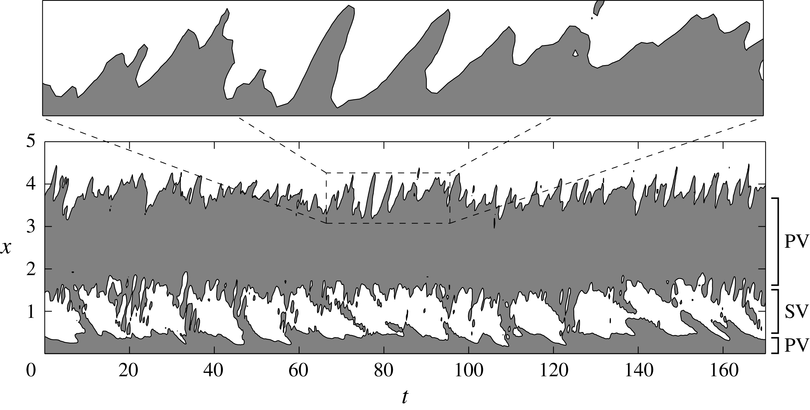
The space–time contours of the spanwise-averaged wall shear stress in figure 5 allow us to also analyse the large-scale behaviour of the secondary vortex, which can be recognized as the region of forward flow, $\hat{\unicode[STIX]{x1D70F}}_{w}>0$ (white region), in between the reverse flow, $\hat{\unicode[STIX]{x1D70F}}_{w}<0$ (grey region), induced by the primary vortex. An oscillatory pattern can be recognized consisting of long periods of the order of $t\approx 25$ where the secondary vortex takes place, thus interrupting the attached reverse flow of the primary vortex. These periods are alternated with smaller time spans where, in contrast, the reverse boundary layer induced by the primary vortex remains attached to the wall, thus forming bridges of negative shear stress continuously flowing upstream with an average velocity $U_{\unicode[STIX]{x1D70F}}\approx -0.14$ (measured as the slope of the connected regions of reverse flow). The average width of these connected regions of reverse flow is of the order of $t\approx 8$ . During this time window, the spanwise averaged secondary vortex is very weak or even absent. The overall picture is as follows. The primary vortex induces a reverse boundary layer that, under the effect of the previously shown adverse pressure gradient, detaches, giving rise to the secondary vortex. The lifetime of this reverse flow detachment and, hence, of the secondary vortex is recognized to be of the order of $t\approx 25$ . These long periods are alternated with shorter time windows, $t\approx 8$ , during which the reverse boundary layer no longer detaches forming a bridge of negative shear stress toward the leading-edge region. As will be shown in § 7, this phenomenon, in conjunction with intermittent events of upstream advection, is induced by favourable pressure gradient conditions. Let us finally point out that the lifetime of the secondary vortex, $t\approx 25$ , corresponds to a very-large-scale phenomenon which embraces the entire flow and will hereafter be referred to as the very-large-scale unsteadiness of the flow. Given the clear matching of temporal scales with the low-frequency unsteadiness found in Kiya & Sasaki (Reference Kiya and Sasaki1985) for a flat plate, and in Le et al. (Reference Le, Moin and Kim1997) for a backward-facing step, such a large-scale phenomenon is conjectured to be an inherent general feature of separating and reattaching flows.

5 Three-dimensional spatial correlation function

The statistical signature of the previously described flow pattern can be studied by means of two-point statistics, such as the velocity correlation function in physical space. This allows us to identify the statistically dominant three-dimensional structures of the flow and to quantitatively assess their topology. For the symmetries of the flow, the spatial correlation function for a generic quantity $\unicode[STIX]{x1D6FD}$ can be defined as

(5.1) $$\begin{eqnarray}R_{\unicode[STIX]{x1D6FD}\unicode[STIX]{x1D6FD}}(x,y,r_{x},r_{y},r_{z})=\frac{\langle \unicode[STIX]{x1D6FD}^{\prime }(x,y,z,t)\unicode[STIX]{x1D6FD}^{\prime }(x+r_{x},y+r_{y},z+r_{z},t)\rangle }{\langle \unicode[STIX]{x1D6FD}^{\prime }\unicode[STIX]{x1D6FD}^{\prime }\rangle (x,y)}.\end{eqnarray}$$

Equation (5.1) emphasizes that the correlation function is defined in a five-dimensional compound space of separations $(r_{x},r_{y},r_{z})$ and positions $(x,y)$ . For each position $(x,y)$ within the flow, the spatial correlation function allows us to define the lengths $(r_{x},r_{y},r_{z})$ of the statistically dominant coherent motions. Owing to statistical inhomogeneity in the streamwise and vertical directions, the three-dimensional spatial correlation function (5.1) is symmetric only in the $r_{z}$ -direction, i.e.  $R_{\unicode[STIX]{x1D6FD}\unicode[STIX]{x1D6FD}}(x,y,r_{x},r_{y},r_{z})=R_{\unicode[STIX]{x1D6FD}\unicode[STIX]{x1D6FD}}(x,y,r_{x},r_{y},-r_{z})$ . For obvious reasons of compactness, only three reference locations of the $(x,y)$ -space will be shown as representatives of the primary vortex shedding region, the attached reverse boundary layer and the detached reverse boundary layer, respectively. In describing the correlation lengths, we will use $\ell _{j}$ to denote the size of a given three-dimensional correlation isosurface along the $j$ direction and $d_{j}$ to denote the distance between peaks of positive and negative correlation. For a similar analysis, the reader is referred to Sillero, Jiménez & Moser (Reference Sillero, Jiménez and Moser2014) where three-dimensional spatial correlation is used to study the structures of turbulent boundary layers and channels.

5.1 Primary vortex shedding region

Figure 6.

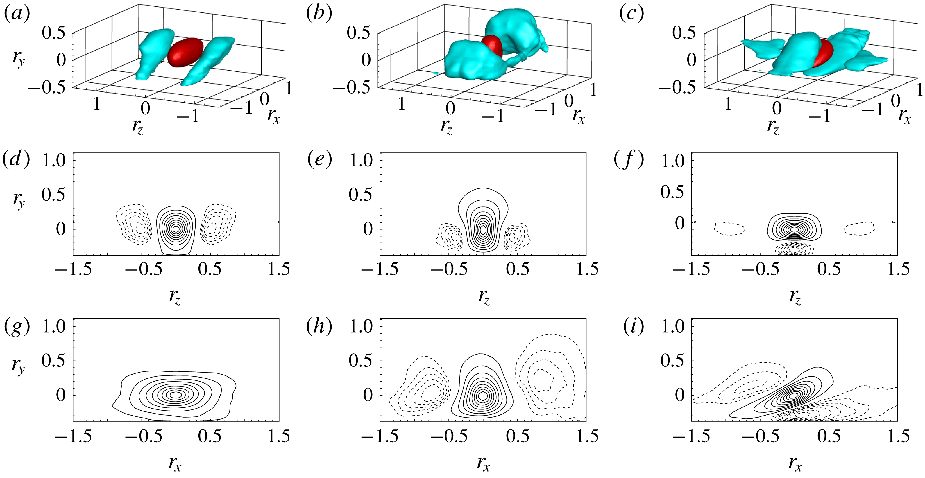
Three-dimensional spatial correlation functions evaluated in the primary vortex shedding region at $(x,y)=(4,0.39)$ corresponding to location P4 highlighted in figure 2(a). The spatial correlation is computed for the streamwise (a,d,g), vertical (b,e,h) and spanwise (c,f,i) velocity fluctuations, i.e.  $R_{uu}$ , $R_{vv}$ and $R_{ww}$ , respectively. Panels (a–c) show a three-dimensional view of the $(r_{x},r_{y},r_{z})$ -space by means of two isosurfaces of positive and negative correlation, i.e. for $R_{uu}=R_{vv}=R_{ww}=0.3$ (red) and for $R_{uu}=R_{vv}=R_{ww}=-0.06$ (cyan), respectively. Panels (d–f) and (g–i) show a two-dimensional section of the isolevels of velocity correlations for $r_{x}=0$ and $r_{z}=0$ , respectively. The positive correlation range of values is discretized by nine equally spaced isolevels (solid lines) whereas the negative range is discretized by five equally spaced isolevels (dashed lines).

We start the analysis by considering the behaviour of the velocity spatial correlation function in the primary vortex shedding region at $(x,y)=(4,0.39)$ corresponding to location P4 highlighted in figure 2(a). In this region, the increment in the vertical direction $r_{y}$ is limited by the presence of the rectangular plate so that $r_{y}>-0.39$ since for $r_{y}\leqslant -0.39$ the moving point of the correlation $(x+r_{x},y+r_{y},z+r_{z},t)$ would be inside the rectangular plate. The measured maximum and minimum values of correlation are $1.01$ and $-0.37$ , and the correlated and anticorrelated structures are identified here with isosurfaces of correlation $0.3$ and $-0.06$ , respectively.

The three-dimensional correlation of the streamwise velocity fluctuation is shown in figure 6(a,d,g). The positively correlated region, $R_{uu}=0.3$ , has an ellipsoidal shape elongated in the streamwise direction whose lengths are $\ell _{x}\approx 1$ and $\ell _{z}\approx 0.4$ . Concerning the vertical lengths, as better highlighted by the $r_{x}=0$ and $r_{z}=0$ sections, the positive correlation of streamwise velocity is found to extend down to the wall. Two regions of negative correlation are also detected, $R_{uu}=-0.06$ , and are found to flank the positively correlated region in the spanwise direction. These two regions are inclined with respect to the wall so that their upstream root is at the wall and their downstream head points away from it. The cross-flow shape is slightly stretched in the vertical direction, see the section in the $r_{x}=0$ space. In particular, we measure $\ell _{y}\approx 0.45$ and $\ell _{z}\approx 0.4$ . The spanwise distance of their centre to the peak of positive correlation is $d_{z}\approx 0.5$ .

The three-dimensional spatial correlation of the vertical velocity fluctuation is shown in figure 6(b,e,h). In contrast to streamwise fluctuations, the positively correlated region $R_{vv}=0.3$ has a tall shape elongating in the vertical direction. The lengths in the horizontal directions are $\ell _{x}\approx 0.55$ and $\ell _{z}\approx 0.4$ . As shown in the $r_{x}=0$ and $r_{z}=0$ planes, the positive isolevels do not reach the wall, thus highlighting the detached nature of vertical fluctuations. The positive correlation region of vertical fluctuations is found to be flanked both in the streamwise and spanwise directions by negative correlation regions. In the spanwise direction, the negative correlation $R_{vv}=-0.06$ takes the form of two detached, streamwise-elongated structures whose cross-flow lengths are $\ell _{y}\approx 0.3$ and $\ell _{z}\approx 0.2$ . The spanwise distance of their centre to the peak of positive correlation is $d_{z}\approx 0.4$ and is located slightly closer to the wall $d_{y}\approx -0.1$ . On the other hand, the negative correlation regions beside the positive one in the streamwise direction appear to form two large spanwise structures. The upstream one is located roughly at the same wall distance $d_{y}\approx 0$ and its streamwise distance is $d_{x}\approx -0.8$ , whereas the downstream one is centred further away from the wall $d_{y}\approx 0.3$ and for $d_{x}\approx 0.9$ .

The spanwise velocity correlation is shown in figure 6(c,f,i). The isosurface of positive correlation, $R_{ww}=0.3$ , has an inclined disc-shaped structure. The cross-flow lengths are $\ell _{y}\approx 0.28$ and $\ell _{z}\approx 0.56$ . As shown in the $r_{z}=0$ plane, the upstream values of positive correlations extend down to the wall. The positive correlation is flanked by four negative correlation structures, $R_{ww}=-0.06$ . The strongest anticorrelated structures are those above and below the positive one. The outer structure is detached from the wall and is centred more upstream and away from the wall than the positive correlated region, $d_{x}\approx -0.6$ and $d_{y}\approx 0.15$ . On the other hand, the inner structure is attached to the wall and $d_{x}\approx 0.1$ and $d_{y}\approx -0.3$ . Two weaker anticorrelated regions flank the positive correlation in the spanwise direction for $d_{z}\approx 0.9$ . These two structures are not inclined and are clearly detached from the wall since their vertical length, $\ell _{y}=0.3$ , is small compared with the wall distance.

Summarizing, the spatial organization of the three-dimensional velocity correlation, consisting of negative correlation regions flanking the positive ones in the spanwise direction for the vertical velocity and in the vertical direction for the spanwise one, suggests that the dominant flow structures of this region are quasi-streamwise vortices whose cross-flow lengths are of the order of $d_{y}\approx 0.3$ and $d_{z}\approx 0.4$ . Furthermore, the spanwise flanking of positive and negative correlation for the streamwise velocity suggests a streaky pattern consisting of alternating high and low streamwise velocity regions whose size is $d_{z}\approx 0.5$ . The presence of negative correlation regions beside the positive correlation of vertical velocity in the streamwise direction actually suggests that spanwise rolls are also significant in this region of the flow. The combination of spanwise rolls and streamwise vortices support the previously observed presence of hairpin-like structures, see figures 3 and 4, also from a statistical point of view. The same qualitative behaviour is also observed in the near-wall forward boundary layer region, not shown for brevity reasons. It is intended that the dominant flow structures of the forward boundary layer are again streamwise vortices and streaks as a result of hairpin-like structures.

5.2 Attached reverse boundary layer

In figure 7, we report the behaviour of the spatial correlation function in the attached reverse boundary layer at $(x,y)=(2.7,0.12)$ corresponding to location P3 highlighted in figure 2(a). Also in this region, the increment in the vertical direction $r_{y}$ is limited by the presence of the rectangular plate so that $r_{y}>-0.12$ . The measured maximum and minimum values of correlation are $1.06$ and $-0.41$ , and the correlated and anticorrelated structures are identified with isosurfaces of correlation $0.3$ and $-0.07$ , respectively.

Figure 7.

Three-dimensional spatial correlation functions evaluated in the attached reverse boundary layer at $(x,y)=(2.7,0.12)$ corresponding to location P3 in figure 2(a). The isosurfaces of positive and negative correlation shown in (a–c) are $R_{uu}=R_{vv}=R_{ww}=0.3$ (red) and $R_{uu}=R_{vv}=R_{ww}=-0.07$ (cyan), respectively. For further details on the structure of the figure, see the caption of figure 6.

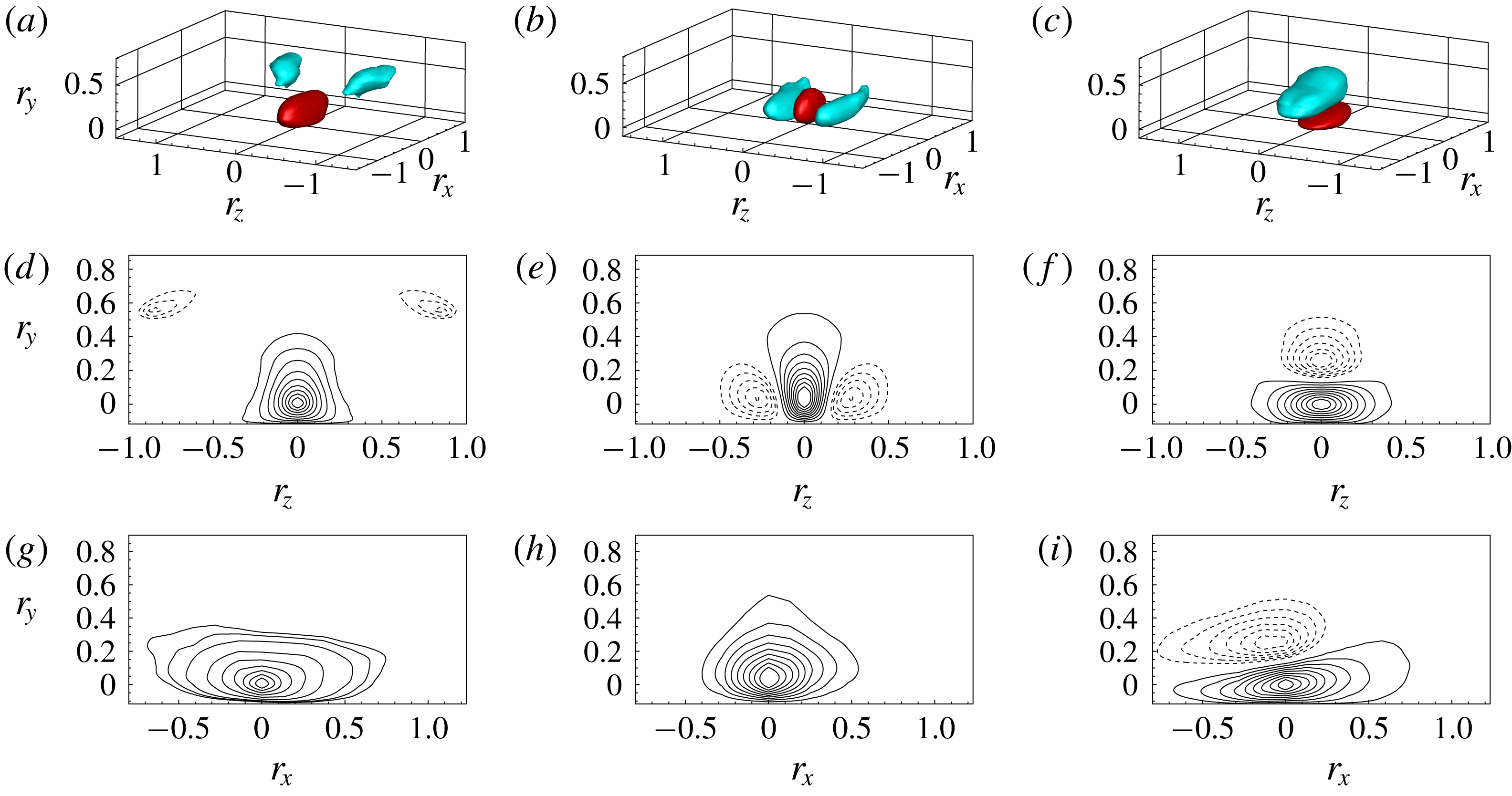
The correlation function of streamwise velocity is shown in figure 7(a,d,g). The isosurface of positive correlation, $R_{uu}=0.3$ , forms a streamwise elongated structure, $\ell _{x}\approx 1$ long and $\ell _{z}\approx 0.34$ wide. As better shown in the $r_{x}=0$ plane, the isolevels of positive correlation extend down to the wall. Two negative correlation regions are also detected, $R_{uu}=-0.07$ . In contrast to the primary vortex shedding region shown in figure 6, the anticorrelated regions are smaller in size and are displaced not only in the spanwise direction but also in the vertical direction. In particular, we measure $d_{y}\approx 0.55$ and $d_{z}\approx 0.85$ .

The correlation of vertical velocity is shown in figure 7(b,e,h). The isosurface of positive correlation, $R_{vv}=0.3$ , forms a slightly elongated structure in the streamwise direction different from the primary vortex shedding region where a tall vertical structure is observed. The horizontal lengths are $\ell _{x}\approx 0.56$ and $\ell _{z}\approx 0.22$ . Two anticorrelated regions, $R_{vv}=-0.07$ , are observed beside the positive correlation in the spanwise direction. These are streamwise elongated structures displaced in the spanwise direction, $d_{z}\approx 0.28$ , and at the same wall distance, $d_{y}\approx 0$ . Their cross-flow lengths are $\ell _{y}\approx 0.27$ and $\ell _{z}\approx 0.25$ .

The correlation of spanwise velocity is shown in figure 7(c,f,i). The isosurface of positive correlation, $R_{ww}=0.3$ , forms a slightly inclined disc-shaped structure whose lengths in the horizontal directions are $\ell _{x}\approx 0.7$ and $\ell _{z}\approx 0.5$ . A single negative correlation region is observed and takes place above the positive one, in contrast to the quadrupole anticorrelation structure observed for the primary vortex shedding region. The isosurface of anticorrelation, $R_{ww}=-0.07$ , takes the form of a slightly inclined structure whose lengths are $\ell _{x}\approx 0.78$ , $\ell _{y}\approx 0.28$ and $\ell _{z}\approx 0.4$ . This structure is displaced in the vertical direction by $d_{y}\approx 0.25$ and in the streamwise direction by $d_{x}\approx -0.08$ .

Overall, the observed anticorrelated regions flanking the correlated ones in the spanwise direction for the vertical velocity and the negative correlation taking place above the positive one for the spanwise velocity suggest that the statistically dominant structures of the attached reverse boundary layer are quasi-streamwise vortices whose cross-flow lengths are $d_{y}\approx 0.25$ and $d_{z}\approx 0.28$ . This result is in accordance with the previous instantaneous flow field analysis, see figure 3(b). The absence of upstream and downstream negative correlations of vertical velocity, as observed in the shedding region, actually suggest that streamwise vortices in the attached reverse flow are not part of the hairpin-like structures. A final difference with respect to the primary vortex shedding region is that the streamwise velocity does not show an evident streaky pattern.

5.3 Detached reverse boundary layer

Figure 8.

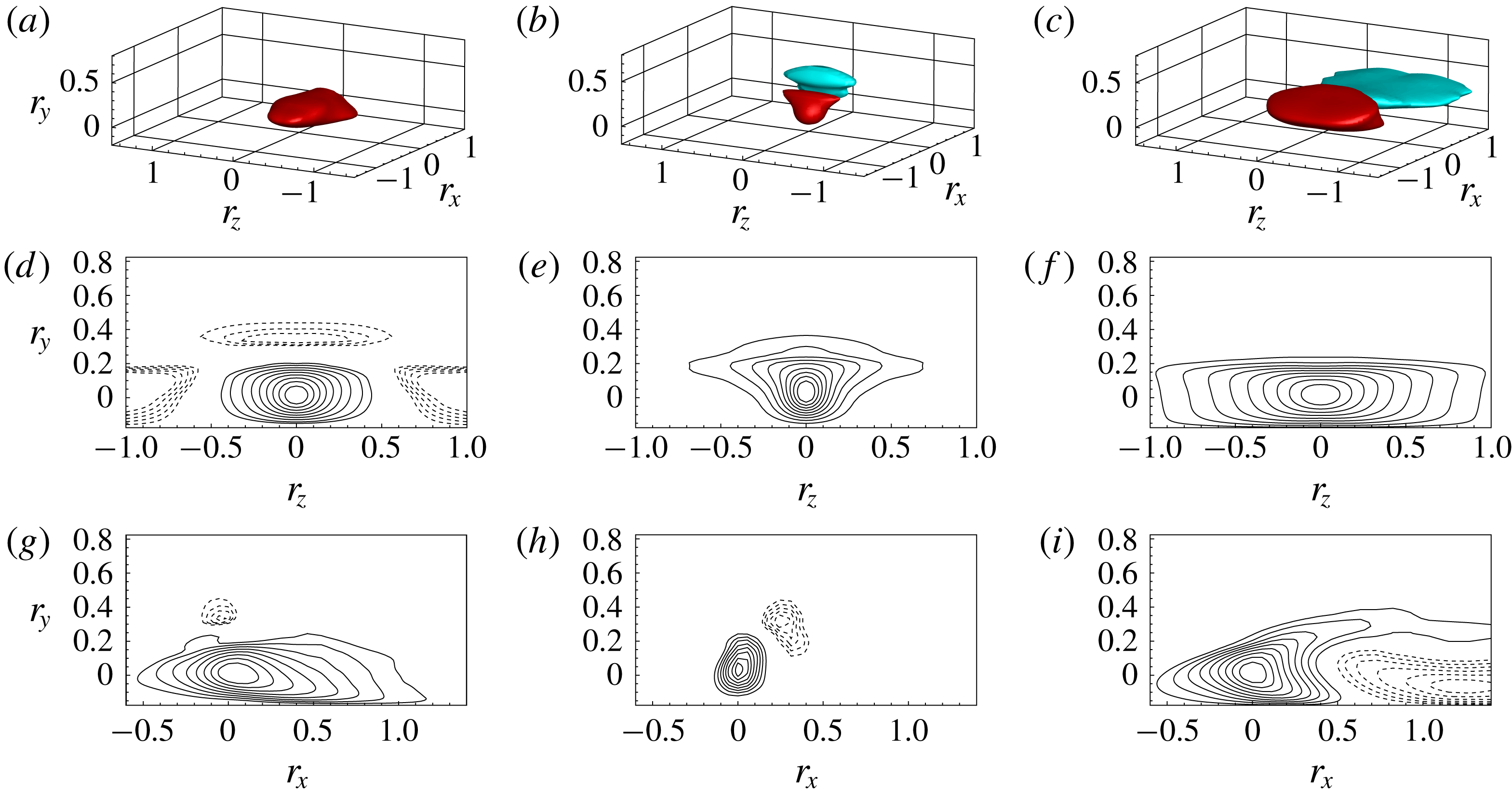
Three-dimensional spatial correlation functions evaluated in the detached reverse boundary layer at $(x,y)=(0.86,0.18)$ corresponding to location P2 in figure 2(a). The isosurfaces of positive and negative correlation shown in (a–c) are $R_{uu}=R_{vv}=R_{ww}=0.3$ (red) and for $R_{uu}=R_{vv}=R_{ww}=-0.2$ (cyan), respectively. For further details on the structure of the figure, see the caption of figure 6.

Here, we analyse the structure of the detached reverse boundary layer by considering the spatial correlation function evaluated at $(x,y)=(0.86,0.18)$ corresponding to location P2 highlighted in figure 2(a). The increment in the vertical direction $r_{y}$ is again limited by the presence of the rectangular plate so that $r_{y}>-0.18$ . The maximum and minimum values of correlation are $1.03$ and $-0.55$ , and the correlated and anticorrelated structures are identified with isosurfaces of correlation $0.3$ and $-0.2$ , respectively.

In figure 8(a,d,g), the three-dimensional correlation function of streamwise velocity is shown. The isosurface of positive correlation $R_{uu}=0.3$ is a compact structure whose horizontal lengths are $\ell _{x}\approx 1$ and $\ell _{z}\approx 0.6$ . No isosurfaces of negative correlation are shown since the anticorrelation of the streamwise velocity is very weak, $\min (R_{uu})=-0.12$ , compared with the other two components of the velocity. However, as shown by the isolevels in the $r_{x}=0$ and $r_{z}=0$ planes, negative correlations are actually present. Although weak, three negative correlation regions are observed with one on the top and two on the spanwise sides of the positive correlation.

The spatial correlation function of the vertical velocity is shown in figure 8(b,e,h). The isosurface of positive correlation, $R_{vv}=0.3$ , is a compact structure stretched in the spanwise direction. Its horizontal lengths are $\ell _{x}\approx 0.29$ and $\ell _{z}\approx 0.6$ . The isosurface of negative correlation, $R_{vv}=-0.2$ , is a small spanwise elongated structure taking place slightly above and downstream from the positive one, $d_{x}\approx 0.25$ and $d_{y}\approx 0.33$ . Its streamwise and vertical lengths are $\ell _{x}\approx 0.22$ and $\ell _{y}\approx 0.28$ .

In figure 8(c,f,i), the three-dimensional correlation function of the spanwise velocity is shown. The isosurface of positive correlation, $R_{ww}=0.3$ , is a large structure elongated in the spanwise direction whose lengths in the wall-parallel directions are $\ell _{x}\approx 0.67$ and $\ell _{z}\approx 1.24$ . The isosurface of negative correlation, $R_{ww}=-0.2$ , is a thin structure taking place downstream of the positive correlation region, $d_{x}\approx 1.2$ and $d_{y}\approx -0.1$ . As clearly shown in the plane $r_{z}=0$ , the isolevels of positive correlation are significantly stretched downstream for large vertical separations. As a consequence, the positive correlation region is found to enclose the region of anticorrelation from above.

Summarizing, the presence of a strong anticorrelated region downstream and slightly above the positive one for the vertical velocity suggests that the dominant structures of the detached reverse boundary layer are spanwise vortices in accordance with the previous analysis of the instantaneous flow field, see figure 3(b). On the other hand, the downstream location and the size of the anticorrelated region for the spanwise velocity suggest the presence of a wall-normal large-scale vortical motion. This motion could be understood as the statistical footprint of the phenomenon reorienting the streamwise vortices of the attached reverse boundary layer into the spanwise vortices observed in the detached reverse boundary layer. Finally, the streamwise velocity does not highlight a spanwise alternating pattern of high- and low-velocity streaks.

6 Multi-scale features

In this section, we address the scale-by-scale evolution of turbulence through the different regions of the flow. To this aim, we study the inhomogeneous behaviour of turbulent spectra. By taking advantage of the statistical homogeneity of the flow in the spanwise direction and in time, the spectrum of a generic quantity $\unicode[STIX]{x1D6FD}$ can be defined as

(6.1) $$\begin{eqnarray}\unicode[STIX]{x1D6F7}_{\unicode[STIX]{x1D6FD}\unicode[STIX]{x1D6FD}}(k_{z},\unicode[STIX]{x1D714},x,y)=\langle \tilde{\unicode[STIX]{x1D6FD}}(k_{z},\unicode[STIX]{x1D714},x,y)\tilde{\unicode[STIX]{x1D6FD}}^{\ast }(k_{z},\unicode[STIX]{x1D714},x,y)\rangle ,\end{eqnarray}$$

where $k_{z}$ and $\unicode[STIX]{x1D714}$ are the spanwise wavenumber and the frequency and $(\tilde{\cdot })$ denotes the Fourier transform with respect to the spanwise direction and time. Let us point out that the Fourier transform in time has been performed using all the temporal signals without using windowing and weighting functions. Accordingly with (6.1), the spectral properties of the flow turn out to be statistically defined in a four-dimensional space of scales and positions $(k_{z},\unicode[STIX]{x1D714},x,y)$ . To simplify the analysis, in the following, we consider separately the one-dimensional wavenumber and frequency spectrum defined as

(6.2a,b ) $$\begin{eqnarray}\unicode[STIX]{x1D6F7}_{\unicode[STIX]{x1D6FD}\unicode[STIX]{x1D6FD}}^{k_{z}}(k_{z},x,y)=\!\int \!\unicode[STIX]{x1D6F7}_{\unicode[STIX]{x1D6FD}\unicode[STIX]{x1D6FD}}(k_{z},\unicode[STIX]{x1D714},x,y)\,\text{d}\unicode[STIX]{x1D714}\quad \text{and}\quad \unicode[STIX]{x1D6F7}_{\unicode[STIX]{x1D6FD}\unicode[STIX]{x1D6FD}}^{\unicode[STIX]{x1D714}}(\unicode[STIX]{x1D714},x,y)=\!\int \!\unicode[STIX]{x1D6F7}_{\unicode[STIX]{x1D6FD}\unicode[STIX]{x1D6FD}}(k_{z},\unicode[STIX]{x1D714},x,y)\,\text{d}k_{z},\end{eqnarray}$$

respectively. Owing to inhomogeneity in the streamwise and vertical directions, the one-dimensional spectra defined above still contain a large amount of information, being a function of the compound three-dimensional space of locations and wavenumbers/frequencies $(x,y,k_{z}/\unicode[STIX]{x1D714})$ . For this reason, we decided to limit the analysis to two selected reduced spaces of $(x,y)$ locations. These two reduced-space locations are defined by tracing the $(x,y)$ positions intercepted by two selected streamlines of mean velocity. Hence, a spectral analysis of the flow along its mean evolution paths is enabled. The statistical study of the multiscale properties of the flow is then reduced to the analysis of a two-dimensional space $(\unicode[STIX]{x1D6FE},k_{z}/\unicode[STIX]{x1D714})$ where $\unicode[STIX]{x1D6FE}$ is the curvilinear coordinate length defined by the mean velocity streamline along its path in the $(x,y)$ space, $\unicode[STIX]{x1D6FE}=\int \text{d}\unicode[STIX]{x1D6FE}$ with $\text{d}\unicode[STIX]{x1D6FE}=\sqrt{\text{d}x^{2}+\text{d}y^{2}}$ .

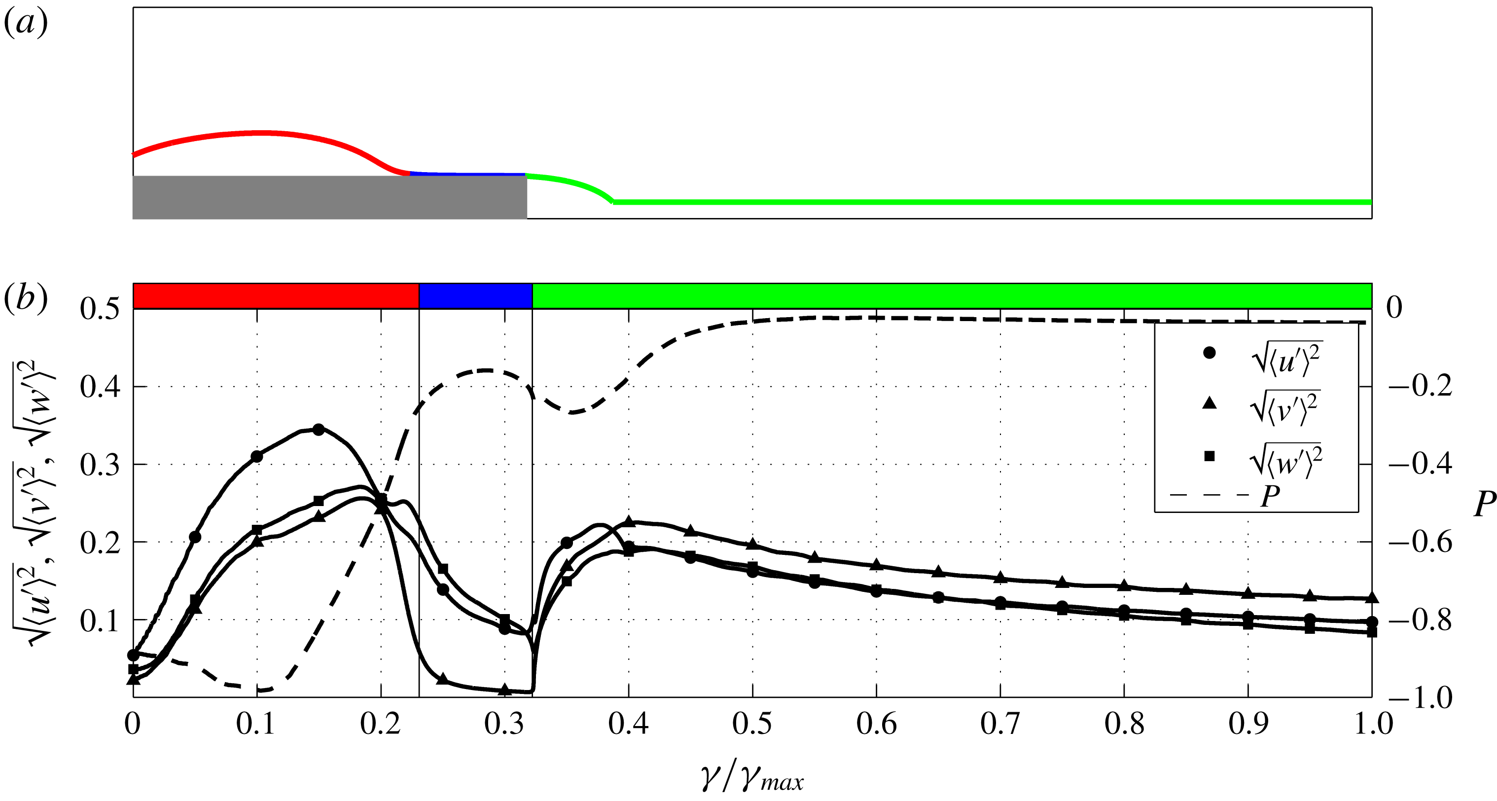
The first reduced space, reported in figure 9(a), is a closed loop tracing the mean flow path around the primary vortex and will hereafter be called the cyclical reduced space. The resulting path $\unicode[STIX]{x1D6FE}$ allows us to study the statistical evolution of the flow along its development in the main recirculating region. Three distinct relevant subregions can be defined. In the first, shown in red in figure 9, we can address how fluctuations are triggered and amplified in the leading-edge shear layer and how they develop during the advection along the primary vortex path up to the reattachment region. In the second part after the reattachment, shown in blue in figure 9, we can deal with the behaviour of the branch of motions flowing upstream through the reverse boundary layer. Finally, in the last part, shown in green in figure 9, we can study the final detached part of the reverse flow up to the leading-edge shear layer, thus closing the cycle. The second reduced space, shown in figure 11(a), starts at the leading edge, covers the primary vortex, reaches the trailing edge and finally moves downstream along the wake. This second reduced space will be called open reduced space and allows us to study the statistical evolution of the flow along its development toward the free flow in the wake. Also in this case, the resulting path $\unicode[STIX]{x1D6FE}$ can be divided into three relevant subregions. The first, in red, traces the evolution of fluctuations from their origin at the leading-edge shear layer up to the reattachment point. The second part, in blue, allows us to assess the behaviour along the attached forward boundary layer, whereas the third, in green, describes the development of the motion along the wake.

In the following, we show spectral results for the vertical velocity component only. The spectra of the other components of velocity and of the pressure field have been also analysed, but are not reported for brevity. However, the main differences, when present, and the main outcomes from the other components of velocity and from the pressure field will be explicitly highlighted in the text.

6.1 The cyclical reduced space

Figure 9.

(a) Selected streamline for the study of the recycling mechanisms in the primary vortex. (b) Behaviour of turbulent intensities and of mean pressure along the path $\unicode[STIX]{x1D6FE}$ .

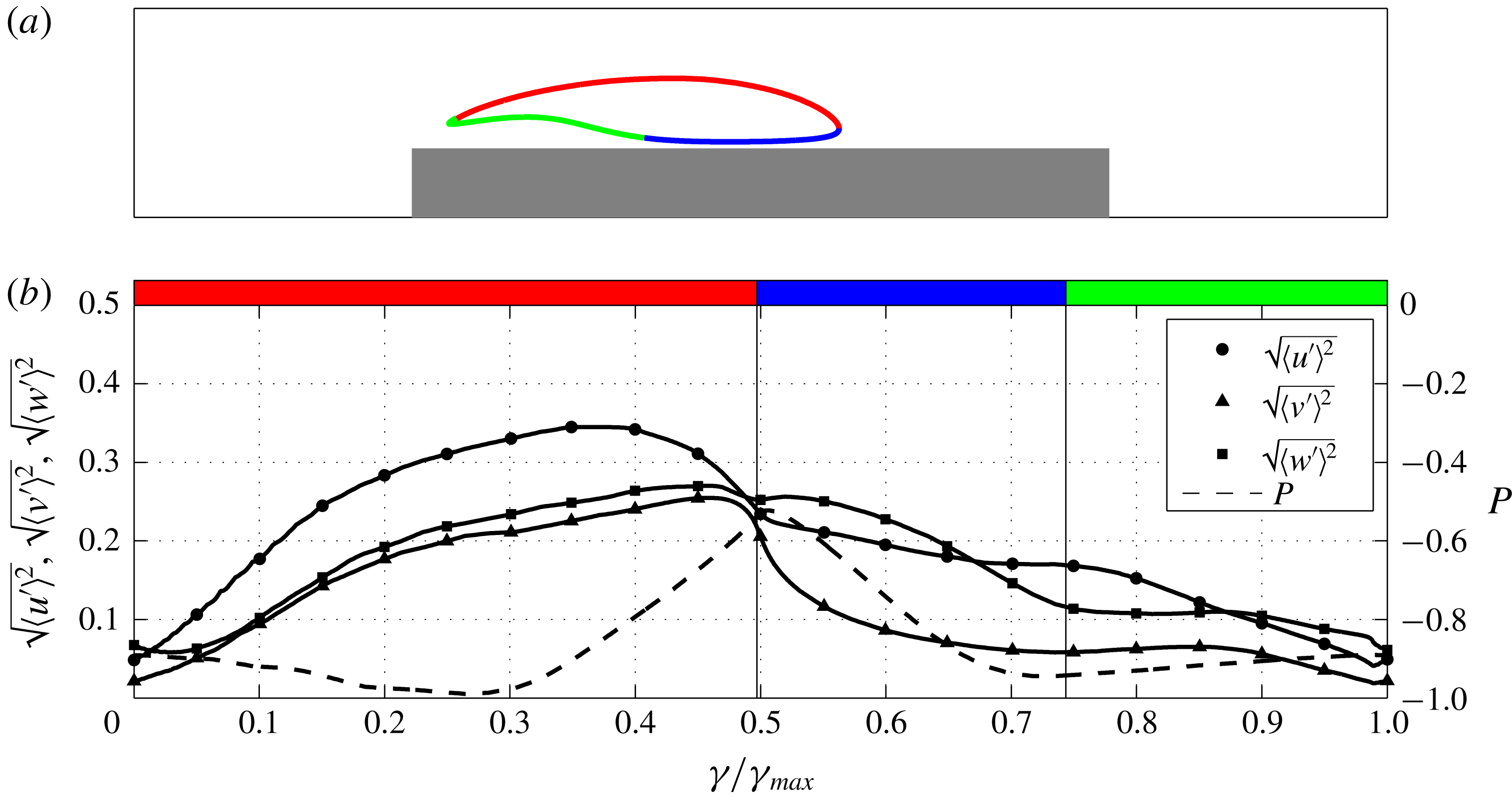
Let us consider the behaviour of the flow in the cyclical reduced space. As reported in figure 9, the mean pressure $P(x,y)$ shows a slight decrease from the leading edge up to the streamwise location of the primary vortex core corresponding to $\unicode[STIX]{x1D6FE}/\unicode[STIX]{x1D6FE}_{max}\approx 0.27$ . Then, the mean pressure field highlights a significant adverse pressure gradient up to the reattachment region for $0.27<\unicode[STIX]{x1D6FE}/\unicode[STIX]{x1D6FE}_{max}<0.5$ . After this region, moving upstream in the reverse boundary layer, the mean pressure field shows an almost equivalent favourable pressure gradient up to $\unicode[STIX]{x1D6FE}/\unicode[STIX]{x1D6FE}_{max}\approx 0.7$ . This streamwise location is the footprint of the low pressure levels associated with the primary vortex core, see also the isocontours of mean pressure shown in figure 2(b). In the final part of the path before reaching back to the leading-edge shear layer, the mean pressure again shows an adverse gradient.

In figure 9, the behaviour of the turbulent intensities, $\langle u^{\prime }u^{\prime }\rangle$ , $\langle v^{\prime }v^{\prime }\rangle$ and $\langle w^{\prime }w^{\prime }\rangle$ is also shown. In the first part of the path (red section) along the leading-edge shear layer, the turbulent intensities increase. Indeed, the free-shear layer is recognized to be the site of the instabilities first and then of the transition to turbulence in this kind of flow. For $\unicode[STIX]{x1D6FE}=0$ , the three components exhibit similar values, but the streamwise fluctuations are found to be the most amplified along the path. The increase of the turbulent intensities is maintained up to the reattachment region with the exception of the streamwise fluctuations, which show a decrease just before it. The result is that in the reattachment region, the intensity of the fluctuations is almost equally distributed in the three directions. After the reattachment, along the reverse boundary layer (blue section), all three components of the turbulent intensities decrease. As expected, owing to the impermeability constraint given by the proximity of the wall, this reduction abruptly occurs for the vertical fluctuations. Interestingly, the most intense fluctuations in the first part of the reverse boundary layer are those in the spanwise direction. This fact could be explained as the result of a spanwise sweeping of the three-dimensional fluctuations impinging into the wall. In the last segment of the path (green section), the intensity of the fluctuations further decreases before reaching the leading-edge shear layer, thus closing the cycle. Such a decrease is most significant for the streamwise fluctuations, presumably due to the adverse pressure gradient that is established in this final part of the path.

Figure 10.

Premultiplied one-dimensional spectra of turbulent vertical fluctuations in the cyclical reduced space. (b) Premultiplied one-dimensional wavenumber spectrum $k_{z}\unicode[STIX]{x1D6F7}_{vv}^{k_{z}}$ as a function of $(\unicode[STIX]{x1D6FE},\unicode[STIX]{x1D706}_{z})$ where $\unicode[STIX]{x1D706}_{z}$ is the spanwise wavelength, $\unicode[STIX]{x1D706}_{z}=2\unicode[STIX]{x03C0}/k_{z}$ . (c) Premultiplied one-dimensional frequency spectrum $\unicode[STIX]{x1D714}\unicode[STIX]{x1D6F7}_{vv}^{\unicode[STIX]{x1D714}}$ as a function of $(\unicode[STIX]{x1D6FE},\unicode[STIX]{x1D706}_{t})$ where $\unicode[STIX]{x1D706}_{t}$ is the period, $\unicode[STIX]{x1D706}_{t}=2\unicode[STIX]{x03C0}/\unicode[STIX]{x1D714}$ . The premultiplied spectra are normalized with their local maxima, e.g.  $k_{z}\unicode[STIX]{x1D6F7}_{vv}^{k_{z}}(\unicode[STIX]{x1D6FE},\unicode[STIX]{x1D706}_{z})/\max (\unicode[STIX]{x1D6F7}_{vv}^{k_{z}}|_{\unicode[STIX]{x1D6FE}})$ , and are shown in linear scale. To address the variation of the intensity of the vertical fluctuations along the path, the reader should refer to figure 9.

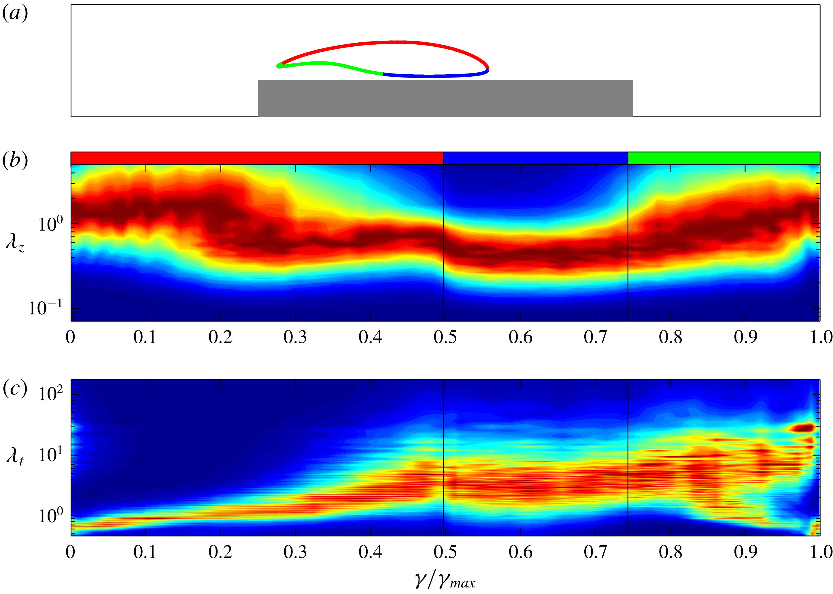
The multiscale nature of the flow in the cyclical reduced space is described by means of turbulent spectra of the vertical velocity and is shown in figure 10. In the very first part of the leading-edge shear layer (red segment), the most energetic spanwise scales of the flow are relatively large, of the order of the rectangular plate thickness, $\unicode[STIX]{x1D706}_{z}=O(1)$ . In contrast, the energy peak in time is located at small time scales of the order of $\unicode[STIX]{x1D706}_{t}=O(10^{-1})$ . In fact, a second distinct peak is present for relatively large time scales of the order of $\unicode[STIX]{x1D706}_{t}=O(10)$ . Its intensity is smaller than the first one located at small time scales. The nature of the second smaller peak at large time scales is analysed in the following section. However, let us note that, interestingly, the intensity of the second peak becomes smaller and smaller with respect to the first when moving downstream along the path and almost disappears around $\unicode[STIX]{x1D6FE}/\unicode[STIX]{x1D6FE}_{max}\approx 0.06$ . These behaviours of the turbulent spectra are in accordance with the presence of spanwise vortex tubes as a result of the Kelvin–Helmholtz instability of the shear layer. In particular, it appears that the mean width of these structures is of the order of the plate thickness.

Figure 11.

(a) Selected streamline for the study of the free flow from the leading edge up to the wake. (b) Behaviour of turbulent intensities and of mean pressure along the path $\unicode[STIX]{x1D6FE}$ .

Following the development of the shear layer, the energy-containing spanwise scales $\unicode[STIX]{x1D706}_{z}$ remain almost unaltered of the order of $O(1)$ , whereas the time scales $\unicode[STIX]{x1D706}_{t}$ increase in accordance with the formation of streamwise vortices due to the stretching and reorientation by mean shear of the spanwise tubes to form hairpin-like patterns. This behaviour is retained up to $\unicode[STIX]{x1D6FE}/\unicode[STIX]{x1D6FE}_{max}\approx 0.2$ where a decrease of the most energetic spanwise scales $\unicode[STIX]{x1D706}_{z}$ starts to take place, and the temporal scales $\unicode[STIX]{x1D706}_{t}$ continue to increase. In fact, in a very short length, from $\unicode[STIX]{x1D6FE}/\unicode[STIX]{x1D6FE}_{max}\approx 0.2$ to ${\approx}0.3$ , the energy-containing spanwise scales decrease to scales of the order of $O(10^{-1})$ . In this short region, transition to turbulence definitely takes place as is also shown by the levels of turbulent kinetic energy reported in figure 2(c). For $\unicode[STIX]{x1D6FE}/\unicode[STIX]{x1D6FE}_{max}>0.3$ and, hence, after the streamwise location of the primary vortex core, the peak of the turbulent spectrum remains at almost the same spanwise scales, whereas the time scales still show a slight increase. The main aspect is a filling of the spectrum, which is particularly marked in the time scales. This behaviour is retained up to the reattachment region. Across the reattachment region, in between the red and blue segments of the path, the spanwise scales become smaller, whereas the time scales remain almost unaltered. This decrease of the spanwise lengths across the reattachment region suggests that structures with smaller spanwise lengths are those mainly advected upstream through the reverse boundary layer. Accordingly, through the analysis of the instantaneous reverse flow pattern, figure 3(b), and of the spatial correlation function, figure 7, these structures are recognized to be streamwise vortices.

Through the reverse boundary layer (blue segment), the most energetic spanwise and temporal scales remain almost unaltered. As shown in figure 9, this section of the path is characterized by a favourable pressure gradient up to the streamwise location of the primary vortex core, $\unicode[STIX]{x1D6FE}/\unicode[STIX]{x1D6FE}_{max}\approx 0.7$ . Further upstream (final part of the blue segment), a weak adverse pressure gradient takes place leading to a longitudinal shrinking and spanwise enlargement of flow structures as shown by the instantaneous reverse flow pattern shown in figure 3(b). Accordingly, we observe an increase of the most energetic spanwise scales, $\unicode[STIX]{x1D706}_{z}$ . Upon entering the last part of the path (green segment), the reverse boundary layer detaches, thus forming the secondary vortex, and the enlargement of flow structures is even more evident, thus leading to spanwise vortices as shown by the spatial correlation function, figure 7 (see also the instantaneous reverse flow pattern shown in figure 3 b). This increase of the most energetic spanwise lengths is retained up to the leading-edge shear layer where the detached spanwise vortices are encompassed by and conform with the even larger motion, $\unicode[STIX]{x1D706}_{z}=O(1)$ , related to the Kelvin–Helmholtz instability, thus closing the cycle. On the other hand, the temporal scales show a very interesting double feature along the detached reverse boundary layer. When moving upstream, for $\unicode[STIX]{x1D6FE}/\unicode[STIX]{x1D6FE}_{max}>0.8$ , the turbulent spectrum splits into two branches of energetic scales. A large time scale range of the order of $O(10)$ characteristic time scales is developed simultaneously with the generation of a small time scale range of the order of $O(10^{-1})$ characteristic time scales. These two branches survive along the detached reverse boundary layer and reach the leading-edge shear layer where only the range of small time scales survives, thus closing the cycle.

6.2 The open reduced space

The behaviour of the flow in the open reduced space is shown in figure 11. We again start the analysis by considering the behaviour of the mean pressure field. The first part of the path (red segment) essentially matches the corresponding section of the cyclical reduced space. Indeed, pressure is found to slightly decrease up to the streamwise location of the primary vortex core, then it starts to increase. In contrast to what happens in the cyclical reduced space, this adverse pressure gradient is also maintained in the second part of the path (blue segment). Indeed, this second part corresponds to the forward boundary layer toward the trailing edge. The mean pressure rise is observed up to $\unicode[STIX]{x1D6FE}/\unicode[STIX]{x1D6FE}_{max}\approx 0.28$ where it leaves room for a small favourable pressure gradient which continues in the first part of the last section of the path (green segment). From a relative minimum immediately after the trailing edge around $\unicode[STIX]{x1D6FE}/\unicode[STIX]{x1D6FE}_{max}\approx 0.36$ , the mean pressure field increases again up to the free stream value in the wake just after a few lengths for $\unicode[STIX]{x1D6FE}/\unicode[STIX]{x1D6FE}_{max}\approx 0.5$ .

As shown in figure 11, from the instabilities in the very first part of the leading-edge shear layer, the turbulent intensities grow while moving around the primary vortex (red segment). A drastic decrease is then observed when approaching the reattachment region, especially for the wall-normal fluctuations. This decrease of the fluctuations is almost maintained in the forward boundary layer (blue segment) up to the trailing edge where a second shear layer forms and develops in the wake, thus promoting the generation of turbulent fluctuations. Indeed, in the very first part of the wake (green segment) a strong increase in the fluctuations is observed, especially for the vertical component. This growth is maintained for a very short length up to $\unicode[STIX]{x1D6FE}/\unicode[STIX]{x1D6FE}_{max}\approx 0.4$ and just downstream from the average wake vortex, a weak decrease of the fluctuations takes place following the asymptotic behaviour of the wake.

Figure 12.

Premultiplied one-dimensional spectra of turbulent vertical fluctuations in the open reduced space. See the caption of figure 10.

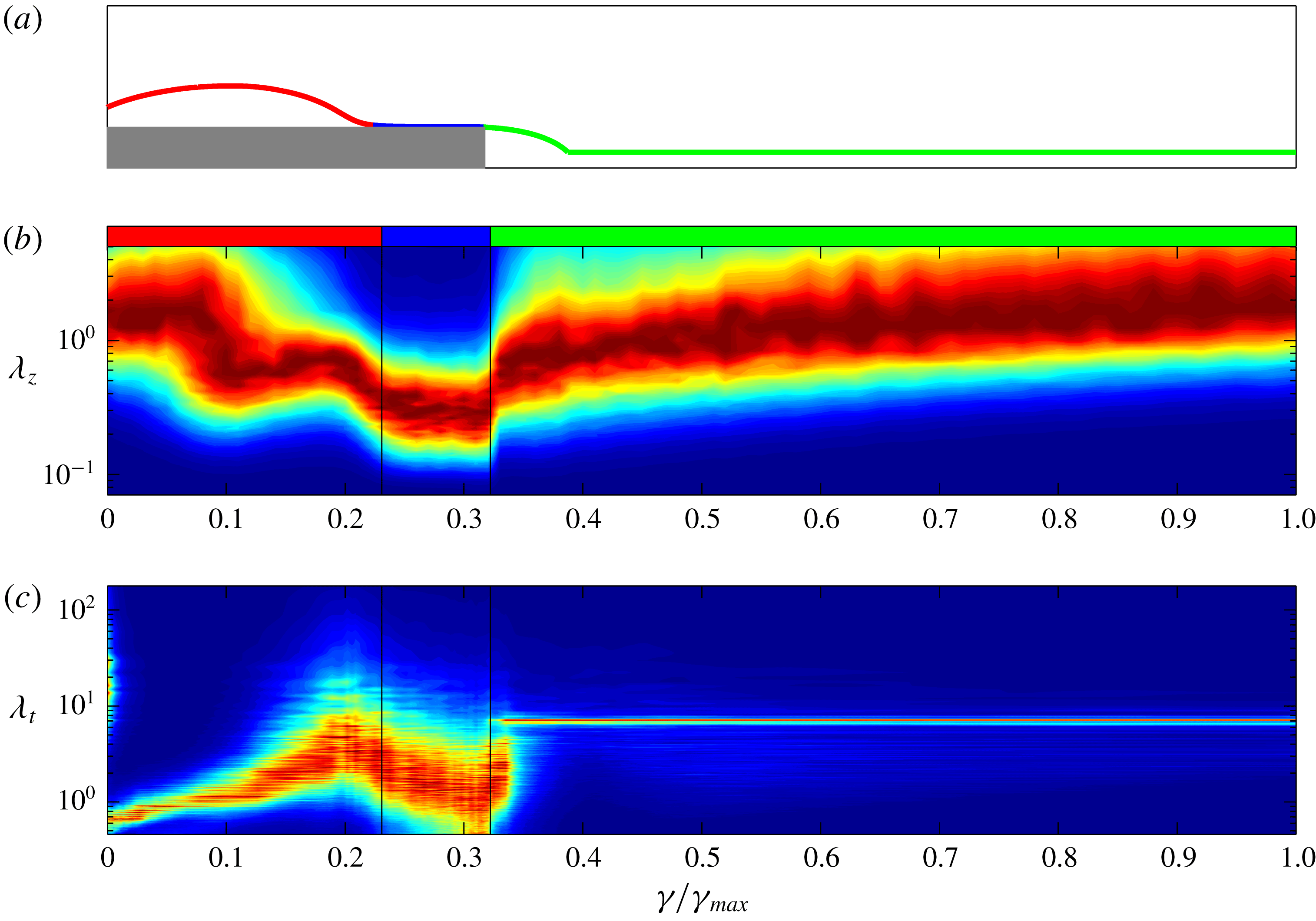
Let us now analyse the multiscale features of the open reduced space reported in figure 12. The first part of the path (red segment) essentially matches the corresponding region of the cyclical reduced space and will be not described for brevity reasons. We start then by considering the second part of the path (blue segment), i.e. from the reattachment region down to the trailing edge. By crossing the reattachment region, a significant decrease of the most energetic spanwise and temporal scales is observed. Then, following the development of the forward boundary layer, the spanwise scales remain almost unchanged, whereas the temporal scales decrease. By crossing the trailing edge, the relatively small spanwise and temporal scales of the boundary layer are abruptly encompassed by the large-scale motion of the separated wake. Interestingly, the most energetic spanwise scales rapidly evolve and reach large values of the order $O(1)$ . On the other hand, the temporal scales do not evolve upon passing the trailing edge, but are found to be simply damped in a very short length for $\unicode[STIX]{x1D6FE}/\unicode[STIX]{x1D6FE}_{max}<0.35$ . Indeed, the dynamics of the wake create a separate well-defined peak at larger temporal scales, $\unicode[STIX]{x1D706}_{t}\approx 7$ , i.e. the shedding time scale. Hence, for $\unicode[STIX]{x1D6FE}/\unicode[STIX]{x1D6FE}_{max}>0.35$ only the large-scale motions of the wake survive and the resulting spectrum is not fulfilled in contrast to the spectrum in the spanwise scales. Let us close the analysis of the open reduced space by addressing the spectral evolution of the wake for $\unicode[STIX]{x1D6FE}/\unicode[STIX]{x1D6FE}_{max}>0.4$ . A logarithmic (linear in the semilog plot) increase of the spanwise scales and a replenishment of the spectral bands is observed. The same development of wake turbulence cannot be observed in the temporal scales owing to the intensity of the shedding spectral peak which overshadows the energy content of the other spectral bands.

7 Self-sustaining cycle

Before discussing the self-sustaining mechanisms of the flow, it is instrumental to briefly recall the main features of the separating and reattaching flows analysed so far. In the very first part of the leading-edge shear layer, the instability of the flow gives rise to very large spanwise vortex structures. The interaction with the strong shear leads to a blow up and streamwise stretching of these structures, thus giving rise to a hairpin-like flow pattern and to the development of streamwise vortices and high- and low-speed streaks. Hence, transition to turbulence takes place, as highlighted by the levels of the turbulent intensities and by the filling of the turbulent spectrum shown in figures 9 and 10. Two branches of turbulent structures can be identified. The first represents detached fluctuations that are freely convected downstream toward the wake. The second is given by turbulent structures moving down toward the wall. These fluctuations impinge into the wall and a portion of these flows downstream toward the trailing edge while the other portion moves upstream, thus forming a reverse boundary layer.

This last branch of turbulent structures accelerates first, driven by a favourable pressure gradient associated with the low-pressure levels of the primary vortex core, see the behaviour of pressure within the blue segment shown in figure 9. These structures are found to be essentially elongated in the streamwise direction as shown by the analysis of the correlation function (figure 7). Then, beyond the streamwise location of the primary vortex core, the reverse boundary layer experiences an adverse pressure gradient and detaches, thus forming a secondary vortex. In the consequent detached reverse boundary layer, turbulent fluctuations become wider and wider as shown again by the analysis of the correlation function (figure 8). These spanwise vortices are eventually conveyed upstream thus triggering the leading-edge shear layer and closing the cycle. In the following, we provide evidence of a self-sustaining cycle at the base of the upstream rising of these spanwise vortices and, hence, of the triggering of the leading-edge shear layer instabilities.

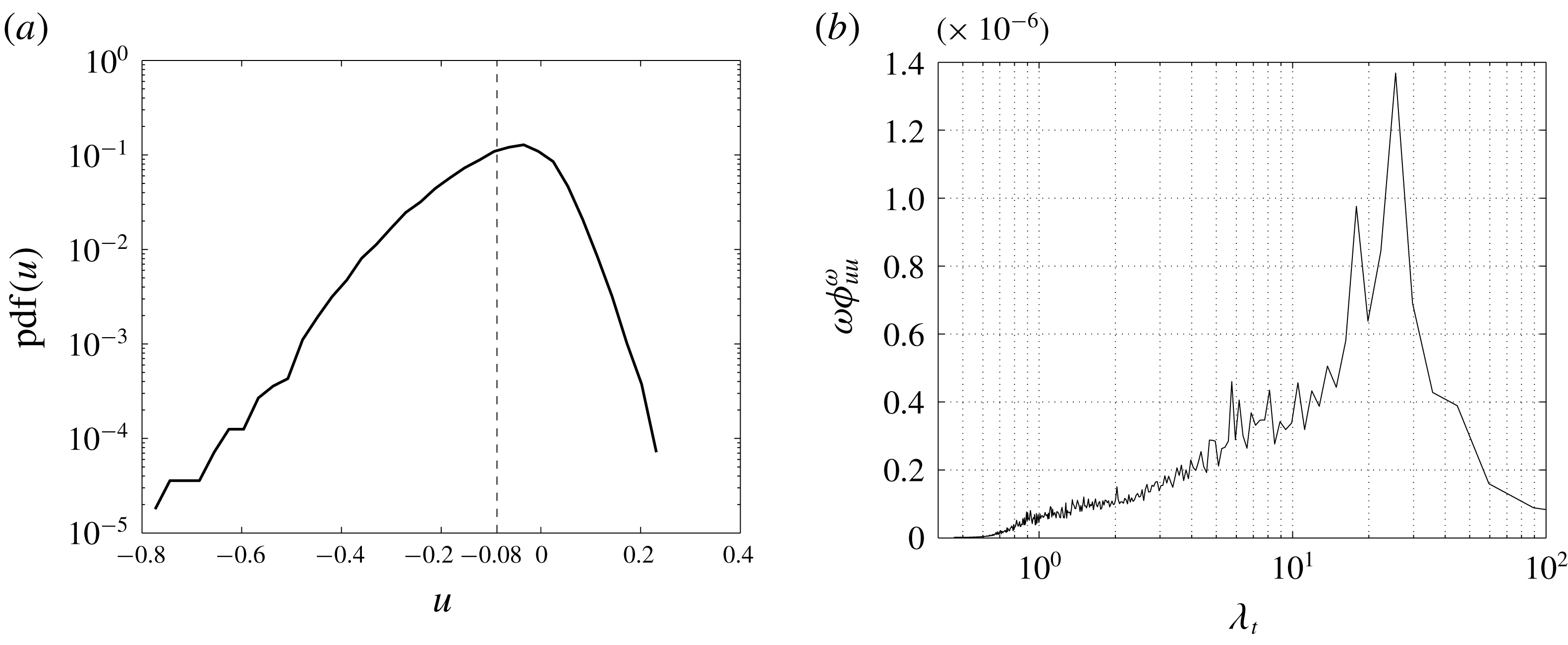
A careful inspection of the detached reverse boundary layer reveals that the mean upstream advection of turbulent fluctuations is very weak in this region. Figure 13(a) reports the probability density function of the streamwise velocity in the detached reverse flow at $(x,y)=(0.88,0.18)$ , corresponding to location P2 shown in figure 2(a). A clear non-Gaussian behaviour is observed. In particular, the flow is recognized to be almost quiescent most of the time. Indeed, as shown by the long negative tail of $\text{pdf}(u)$ , the reverse flow is found to be essentially given by rare and intense events of upstream advection. In accordance with the peak in the premultiplied frequency spectrum of streamwise velocity shown in figure 13(b), these extreme reverse flow fluctuations belong to long time-scale motions of the order of $\unicode[STIX]{x1D706}_{t}\approx 25$ . As a consequence of these periods of quiescence, we recognize that turbulent structures moving upstream from the reattachment region are actually clustered in correspondence of the streamwise location of the secondary vortex because the upstream advection is null for long periods. We argue that this clustering of structures in the detached reverse flow would give rise to vortex reconnection phenomena, which would explain the creation of spanwise vortices from the streamwise ones observed in the attached reverse flow, see the instantaneous flow field analysis, figure 3(b), and the results of the spatial correlation function, figures 7 and 8.

Figure 13.

(a) Probability density function and (b) premultiplied frequency spectrum of the streamwise velocity computed in the reverse flow region at $(x,y)=(0.88,0.18)$ corresponding to location P2 shown in figure 2(a). The dashed vertical line in (a) denotes the mean.

Given the clear matching of temporal scales, this intermittent phenomenon of upstream advection is strictly related to the behaviour of the secondary vortex. Indeed, as shown in figure 5, the time scale between two bridges of negative wall shear stress, i.e. the lifetime of the secondary vortex, is $t\approx 25$ , actually matching the time scale of the upstream advection in the detached boundary layer, $\unicode[STIX]{x1D706}_{t}\approx 25$ , shown in figure 13(b). Both the lifetime of the secondary vortex and the intermittency of the upstream advection of the detached boundary layer are due to events of favourable pressure gradient conditions that, in turn, are given by large-scale unsteadiness phenomena. In particular, we argue that the long periods of quiescence of the detached boundary layer are due to the adverse pressure gradient that for long time scales significantly opposes the weak reverse flow also inducing a detachment of the boundary layer and, hence, creating the secondary vortex. On the other hand, for smaller periods, the adverse pressure gradient becomes weaker, thus allowing the reverse flow to proceed toward the leading-edge shear layer and preventing the flow separation into the secondary vortex.

Figure 14.

(a) Premultiplied frequency spectrum of the streamwise movement of low pressure levels at the wall, $\unicode[STIX]{x1D714}\unicode[STIX]{x1D6F7}_{x_{low}x_{low}}^{\unicode[STIX]{x1D714}}$ . Inset: premultiplied frequency spectrum of vertical velocity, $\unicode[STIX]{x1D714}\unicode[STIX]{x1D6F7}_{vv}^{\unicode[STIX]{x1D714}}$ , evaluated in the wake at a location corresponding to point P5 shown in figure 2(a). (b) Correlation function $R_{x_{low}^{t}x_{low}^{b}}(\unicode[STIX]{x1D70F})$ , equation (7.3).

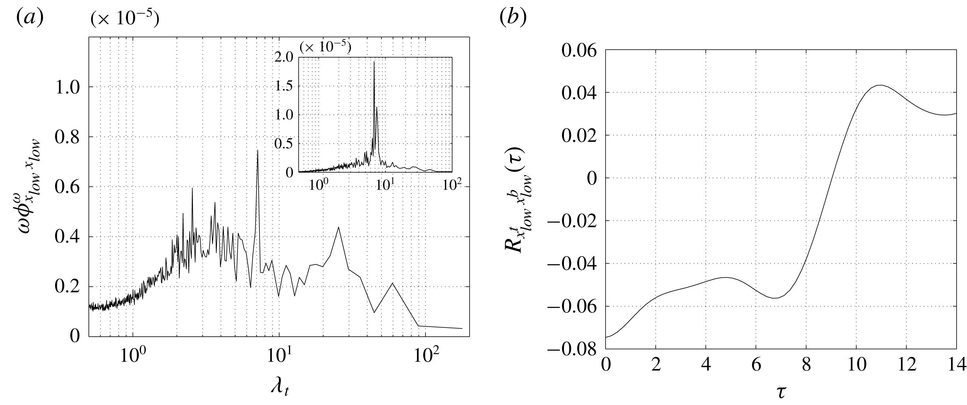
To clarify this point, let us consider the frequency spectrum of the streamwise location of an isolevel of low pressure evaluated at the wall defined as

(7.1) $$\begin{eqnarray}\unicode[STIX]{x1D6F7}_{x_{low}x_{low}}^{\unicode[STIX]{x1D714}}(\unicode[STIX]{x1D714})=\int \langle \tilde{x}_{low}(k_{z},\unicode[STIX]{x1D714})\tilde{x}_{low}^{\ast }(k_{z},\unicode[STIX]{x1D714})\rangle \,\text{d}k_{z},\end{eqnarray}$$

where $x_{low}=x_{low}(z,t)$ is computed as the upstream streamwise location satisfying the following condition

(7.2) $$\begin{eqnarray}p_{wall}(x_{low},z,t)=p_{low},\end{eqnarray}$$

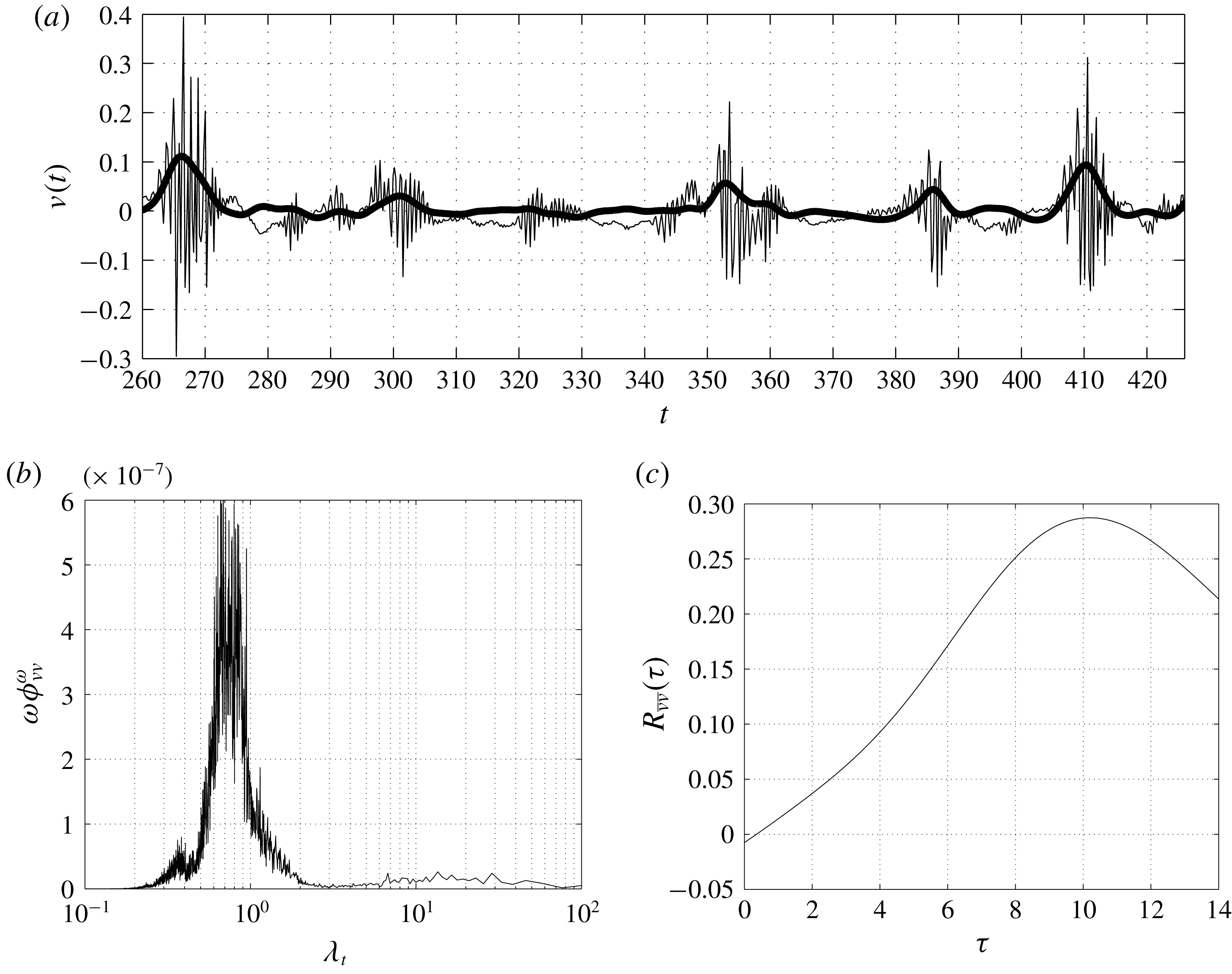
where $p_{low}\equiv 0.45P_{min}=-0.014$ . In figure 14(a) the premultiplied frequency spectrum $\unicode[STIX]{x1D714}\unicode[STIX]{x1D6F7}_{x_{low}x_{low}}^{\unicode[STIX]{x1D714}}$ is shown. A well-defined peak at large time scales, $\unicode[STIX]{x1D706}_{t}\approx 7$ , is present, which exactly matches the frequency of the large-scale vortex detachment in the wake, $\unicode[STIX]{x1D706}_{t}\approx 7$ , see the peak of the premultiplied frequency spectrum of the vertical velocity in the wake shown in the inset of figure 14(a). Actually, as already shown in figures 5 and 12, the shedding of large-scale vortices from the primary vortex is also locked at the same time scale. Hence, we conjecture that the characteristic time scale of the streamwise oscillation of low-pressure levels is a footprint at the wall of the shedding of large-scale vortices from the primary vortex whose characteristic time scale is exactly $t\approx 7$ . However, in figure 14(a), a second spectral peak at even larger time scales, $\unicode[STIX]{x1D706}_{t}\approx 25$ , is observed, thus highlighting that the most intense fluctuations of $x_{low}$ for $\unicode[STIX]{x1D706}_{t}\approx 7$ are superimposed to a weaker fluctuation of $x_{low}$ characterized by an even larger period corresponding to almost four times the vortex shedding period, $\unicode[STIX]{x1D706}_{t}\approx 25$ . Let us now consider the temporal cross-correlation between the streamwise location of low wall pressure in the top and bottom sides of the rectangular plate, $x_{low}^{t}$ and $x_{low}^{b}$ , respectively,

(7.3) $$\begin{eqnarray}R_{x_{low}^{t}x_{low}^{b}}(\unicode[STIX]{x1D70F})=\frac{\langle x_{low}^{t\prime }(z,t^{\prime })x_{low}^{b\prime }(z,t^{\prime \prime })\rangle }{\langle x_{low}^{\prime 2}\rangle },\end{eqnarray}$$

where $\unicode[STIX]{x1D70F}=t^{\prime \prime }-t^{\prime }$ . As shown in figure 14(b), $R_{x_{low}^{t}x_{low}^{b}}(\unicode[STIX]{x1D70F})$ shows a clear anticorrelation for $\unicode[STIX]{x1D70F}=0$ , thus highlighting that, on average, an upstream fluctuation of low wall pressure on one side corresponds to a downstream fluctuation on the opposite side. This negative correlation is retained up to $\unicode[STIX]{x1D70F}\approx 9$ . For larger time scales, the correlation becomes positive and reaches a maximum around $\unicode[STIX]{x1D70F}\approx 11$ , which is then recognized to be the period of inversion of the upstream/downstream fluctuations of low pressure in the two sides of the plate. Let us point out that the time scale of the positive maximum of correlation of two signals in phase opposition corresponds to half of the period of the dominant harmonic. Hence, $\unicode[STIX]{x1D70F}\approx 11$ corresponds in spectral space to the peak of $\unicode[STIX]{x1D714}\unicode[STIX]{x1D6F7}_{x_{low}x_{low}}^{\unicode[STIX]{x1D714}}$ at $\unicode[STIX]{x1D706}_{t}\approx 25$ . This fact suggests a superimposition of the intense fluctuations of $x_{low}$ at $\unicode[STIX]{x1D706}_{t}\approx 7$ with those weaker fluctuations at $\unicode[STIX]{x1D706}_{t}\approx 25$ . Summarizing, the low-wall-pressure levels fluctuate in space by following the detachment of large-scale vortices from the primary vortex. This upstream/downstream movement of low pressure is superimposed to a very slow phenomenon such that the most effective upstream fluctuations of $p_{low}$ actually occur for periods corresponding to that of the very-large-scale unsteadiness of the flow, i.e.  $\unicode[STIX]{x1D706}_{t}\approx 25$ .

Figure 15.

(a) Temporal signal and (b) premultiplied frequency spectrum of vertical velocity in the leading-edge shear layer, location P1 of figure 2(a). The thick line in (a) reports the filtered signal (7.4). (c) Correlation function $R_{\bar{v}\bar{v}}(\unicode[STIX]{x1D70F})$ , equation (7.5).

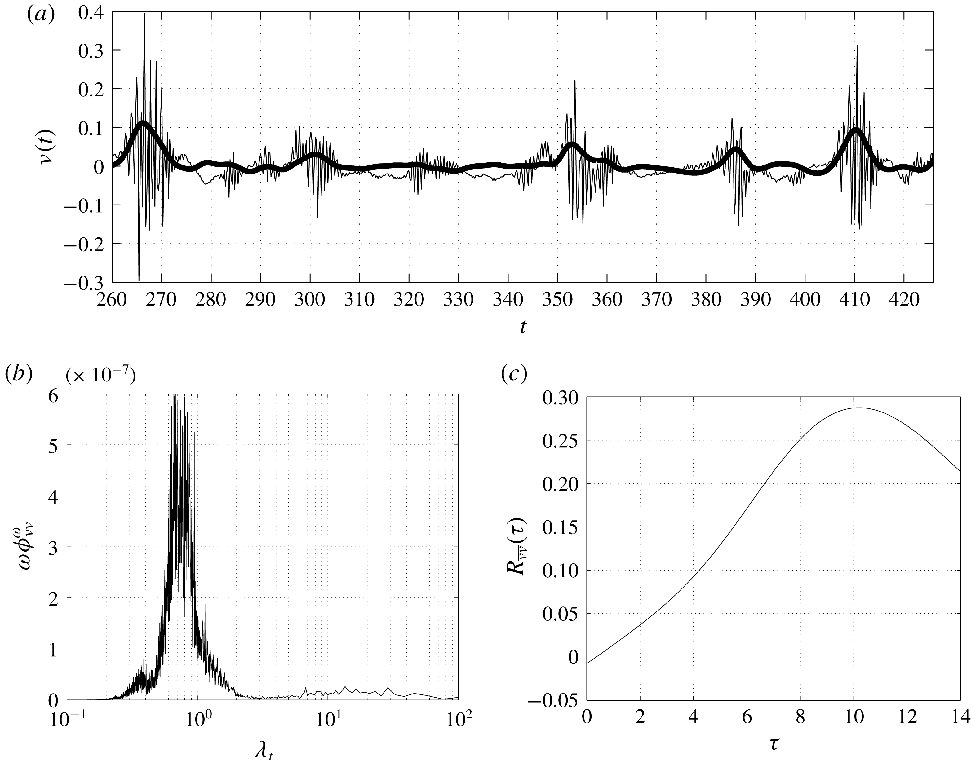
The low-frequency upstream and downstream oscillation of low levels of wall pressure is responsible for the very intermittent upstream advection of turbulent structures within the detached reverse boundary layer shown in figure 13(a). In fact, given the adverse pressure gradient and the small values of momentum associated with the detached reverse boundary layer (green segment of figure 9), turbulent fluctuations are able to reach the leading-edge shear layer only when the pressure levels are favourable, i.e. when $x_{low}\ll \langle x_{low}\rangle$ . Accordingly, the frequency spectrum of streamwise velocity in the detached reverse boundary layer reported in figure 13(b) shows a clear peak at large temporal scales matching the large-scale period of fluctuations of $x_{low}$ at $\unicode[STIX]{x1D706}_{t}\approx 25$ . The same matching of scales is also observed with the characteristic time scale of the secondary vortex shown in figure 5. Given the alternate nature of the process in the two opposite sides of the plate, we argue that turbulent structures along the detached reverse boundary layer are clustered in one side of the plate where the secondary vortex holds and are advected upstream in the opposite side where, in contrast, the secondary vortex is absent or very weak. On average, this clustering and advection is maintained for a relatively long period, and then reverses in the two sides of the plate. In accordance with the peak of correlation shown in figure 14(b), this period of inversion is of the order of $O(10)$ characteristic time scales. Hence, the system consists of trains of small-scale structures able to reach the leading-edge shear alternatively in the two sides of the plate.

In accordance with this picture, the time signals of the fluctuating vertical velocity evaluated in the leading-edge shear layer (location P1 reported in figure 2 a) show packages of high-frequency fluctuations alternating with relative unperturbed periods as shown in figure 15(a). The premultiplied frequency spectrum of vertical velocity shown in figure 15(b) highlights that, on average, these packages are characterized by a range of high frequencies centred at time scales of the order $\unicode[STIX]{x1D706}_{t}\approx 0.7$ . In accordance with the time signal reported in figure 15(a), $\unicode[STIX]{x1D714}\unicode[STIX]{x1D6F7}_{vv}^{\unicode[STIX]{x1D714}}(\unicode[STIX]{x1D714})$ also shows a range of large temporal scales centred at $\unicode[STIX]{x1D706}_{t}\approx 25$ which actually denotes the periodic appearance of these packages. This period matches the large period of the streamwise fluctuations of low wall pressure shown in figure 14(a) and of the upstream advection events in the detached reverse boundary layer shown in figure 13(b), thus supporting the physical connection between pressure fluctuations, upstream advection and triggering of the leading-edge shear layer.

Let us consider the filtered signal of the absolute value of vertical velocity,

(7.4) $$\begin{eqnarray}\bar{v}(x,y,z,t)=\int G_{\unicode[STIX]{x0394}t}(t-t^{\ast })|v(x,y,z,t^{\ast })|\,\text{d}t^{\ast }.\end{eqnarray}$$

As shown in figure 15(a), the filtered signal, with $G_{\unicode[STIX]{x0394}t}$ the Gaussian filter function and with a filter time scale $\unicode[STIX]{x0394}t=4$ , allows us to efficiently detect the packages of small-scale fluctuations triggering the shear layer. By computing the temporal cross-correlation function of the filtered signal (7.4) evaluated in the top and bottom shear layer,

(7.5) $$\begin{eqnarray}R_{\bar{v}\bar{v}}(\unicode[STIX]{x1D70F})=\frac{\langle \bar{v}^{\prime }(x,{\tilde{y}},z,t^{\prime })\bar{v}^{\prime }(x,-{\tilde{y}},z,t^{\prime \prime })\rangle }{\sqrt{\langle \bar{v}^{\prime }\bar{v}^{\prime }\rangle (x,{\tilde{y}})\langle \bar{v}^{\prime }\bar{v}^{\prime }\rangle (x,-{\tilde{y}})}},\end{eqnarray}$$

with $\unicode[STIX]{x1D70F}=t^{\prime \prime }-t^{\prime }$ , we can confirm the alternating nature of the small-scale triggering of the leading-edge shear layer in the top and bottom sides of the rectangular plate. Indeed, as shown in figure 15(c), the trains of small-scale structures detected by the filtered vertical velocity $\bar{v}$ are correlated in the two sides of the plates for $\unicode[STIX]{x1D70F}\approx 11$ matching the time scale of the streamwise rising/descent of low pressure levels along the body. It is worth noting that for $\unicode[STIX]{x1D70F}=0$ , the correlation is almost zero and is not negative as would be expected from a phenomenon of the alternation of two signals. The reason is that the alternation is between quiescence and triggering and, hence, simultaneously ( $\unicode[STIX]{x1D70F}=0$ ) the average product of these two processes in the two shear layers is zero.

We can now give an explanation of the two branches of energetic scales observed previously in § 6 and shown in figure 10. In the final portion of the cyclical reduced-space (green segment of figure 10), the turbulent structures advected upstream through the detached reverse boundary layer have been shown to be spanwise vortices whose spectral footprint is the branch of energetic small temporal scales. On the other hand, the second branch, corresponding to very large temporal scales, can now be understood as the spectral footprint of the observed alternation between the top and bottom sides of long periods of quiescence and rising toward the leading edge of small-scale structures. As a consequence, the second spectral branch is actually a footprint of the very-large-scale unsteadiness of the flow, which promotes/suppresses the upstream rising of packages of small-scale fluctuations toward the leading-edge shear layer through streamwise fluctuations of low pressure levels. Hence, we argue that trains of structures characterized by small time scales and relatively large spanwise lengths, trigger the leading-edge shear layer alternatively in the top and bottom sides for relatively long periods. Indeed, we observe that, while in the first part of the leading-edge shear layer (red segment of figure 10) both spectral branches appear, only the branch of small temporal scales, corresponding to the evolution of the turbulent structures of the reverse boundary layer is amplified.