1. Introduction
The interaction between fluid flow and deformable boundaries is a topic with a wide range of applications including in blood flow, geophysics, biophysics and microrheometry (Vlahovska, Podgorski & Misbah Reference Vlahovska, Podgorski and Misbah2009; Greenwood Reference Greenwood2020). Relative motion between soft surfaces separated by a fluid establishes a lubricated flow capable of supporting lift forces (Johnson Reference Johnson1970; Sekimoto & Leibler Reference Sekimoto and Leibler1993; Beaucourt, Biben & Misbah Reference Beaucourt, Biben and Misbah2004; Skotheim & Mahadevan Reference Skotheim and Mahadevan2004; Urzay, Llewellyn Smith & Glover Reference Urzay, Llewellyn Smith and Glover2007; Szeri Reference Szeri2010; Davies et al. Reference Davies, Débarre, El Amri, Verdier, Richter and Bureau2018) and torques (Rallabandi et al. Reference Rallabandi, Saintyves, Jules, Salez, Schönecker, Mahadevan and Stone2017; Saintyves et al. Reference Saintyves, Rallabandi, Jules, Ault, Salez, Schönecker, Stone and Mahadevan2020), with applications in reducing drag (Dowson & Higginson Reference Dowson and Higginson1959, Reference Dowson and Higginson1966; Saintyves et al. Reference Saintyves, Jules, Salez and Mahadevan2016). While many recent studies consider the case of nearly planar soft surfaces (Snoeijer, Eggers & Venner Reference Snoeijer, Eggers and Venner2013; Essink et al. Reference Essink, Pandey, Karpitschka, Venner and Snoeijer2021; Rallabandi et al. Reference Rallabandi, Oppenheimer, Zion and Stone2018), problems such as the motion of eggs through the oviduct (Bradfield Reference Bradfield1951; Salamon & Kent Reference Salamon and Kent2014), the flow of red blood cells or vesicles through very narrow capillaries (Lighthill Reference Lighthill1968; Fitz-Gerald Reference Fitz-Gerald1969; Vann & Fitz-Gerald Reference Vann and Fitz-Gerald1982; Secomb et al. Reference Secomb, Skalak, Özkaya and Gross1986; Barakat & Shaqfeh Reference Barakat and Shaqfeh2018a; Freund Reference Freund2014) or medical procedures such as vascular intervention (Vurgaft, Elbaz & Gat Reference Vurgaft, Elbaz and Gat2019), require an elastic boundary whose reference state is cylindrical or more generally curved. Introducing a solid object (which in the following we call the intruder) too large to fit into the undeformed cylinder, produces a hoop stress that holds the intruder in place. The ‘dry’ version of this problem (Rallabandi et al. Reference Rallabandi, Marthelot, Jambon-Puillet, Brun and Eggers2019) revealed the interplay between hoop stresses and longitudinal stretching, which is characteristic of the cylindrical geometry. In the present paper we take the tube to be filled with liquid, and apply a force to the intruder (as if pulled by a string), so that thin lubricating liquid layers reduce the friction between the tube and the intruder. Hoop stresses due to the curved boundary, the tension of the membrane, and viscous stresses, are coupled with the pressure of the fluid flow.
To our knowledge, Lighthill (Reference Lighthill1968) was the first to treat a variant of this problem, considering an object (possibly elastic) pushed through an elastic tube by a pressure gradient. Lighthill (Reference Lighthill1968) made a parabolic approximation for the intruder shape, and only considered hoop stresses in his analysis. We will see, below, that even in the limit of low speeds, this is not possible, and stretching of the membrane always comes into play. In subsequent publications (Fitz-Gerald Reference Fitz-Gerald1969; Vann & Fitz-Gerald Reference Vann and Fitz-Gerald1982; Secomb et al. Reference Secomb, Skalak, Özkaya and Gross1986), the pressure-driven model was refined further to account for the specifics of the motion of red blood cells through capillaries, including the effects of asymmetry, the detailed elastic response and the tube porosity. The related problem of pressure-driven motion of close-fitting vesicles in tubes has been analysed using both asymptotic analysis (Barakat & Shaqfeh Reference Barakat and Shaqfeh2018a) and numerical simulations (Barakat & Shaqfeh Reference Barakat and Shaqfeh2018b). By contrast, Chatkoff (Reference Chatkoff1975) considered a different driving mechanism: the motion of ovoids through tubes deforming peristaltically. Takagi & Balmforth (Reference Takagi and Balmforth2011) analysed the peristaltic pumping of a small (i.e. narrower than the tube) object suspended in a fluid-filled tube. Recently, Vurgaft et al. (Reference Vurgaft, Elbaz and Gat2019) considered the flow in an elastic tube due to the insertion of a narrower rigid cylinder.
In this work we focus on the motion of an object as produced by the application of an external force acting along the tube's axis. We approach the problem using lubricated membrane theory, which we develop in detail for slender intruders moving through thin-walled soft tubes, and which we compare with full three-dimensional (3-D) direct numerical simulations (DNS) of the fluid–elastic problem. Our theory accounts for both hoop stresses and membrane stresses in the tube through a geometrically nonlinear theory of the tube elasticity (Sanders Reference Sanders1963; Koiter Reference Koiter1966; Budiansky Reference Budiansky1968) which is coupled to the lubrication pressure in the fluid film. We analyse this framework for intruders with arbitrary axisymmetric shape under both the full membrane theory and a linearized version of it. Performing a systematic asymptotic analysis in the limit of small velocities, we find approximations for the film thickness and the force. The force is found to depend primarily on the slope of the intruder at the leading edge and is only weakly sensitive to other details of its shape. Numerical solutions of the lubricated membrane theory allow us to obtain a quantitative description over the entire parameter space of relative velocity and tube deformation, and over a wide range of intruder shapes. We find good agreement of theory with DNS, in which we solve the full coupled fluid and elastic equations, without assumptions on the membrane thickness. We find that the membrane tension is important even for very slender intruders moving at small speeds.
In § 2 below, we introduce the problem and set up its mathematical structure, starting with a description of the fully coupled fluid–elastic problem to be solved. Section 3 develops the lubricated membrane theory in detail, accounting for tension and hoop stresses in the tube. A simplified version of the theory neglecting tension is analysed in § 4 for arbitrary, but slender, intruder shapes in the singular limit of small speeds. Equipped with insight from this analysis, we then analyse the nonlinear membrane theory in § 5 with asymptotic and numerical methods. Now, the membrane theory is shown to be in excellent agreement with full DNS for the detailed film shape as well as for the force required to drive the intruder at small speeds. Comparison with the hoop-stress model of § 4 reveals a qualitatively different film shape owing to finite tension, even though the effect on the force is small for slender intruders, which can be understood in the asymptotic limit of small speeds. We conclude with a discussion of the validity of the theory and its potential extensions in § 6.
2. Problem formulation
2.1. Problem formulation and numerical implementation
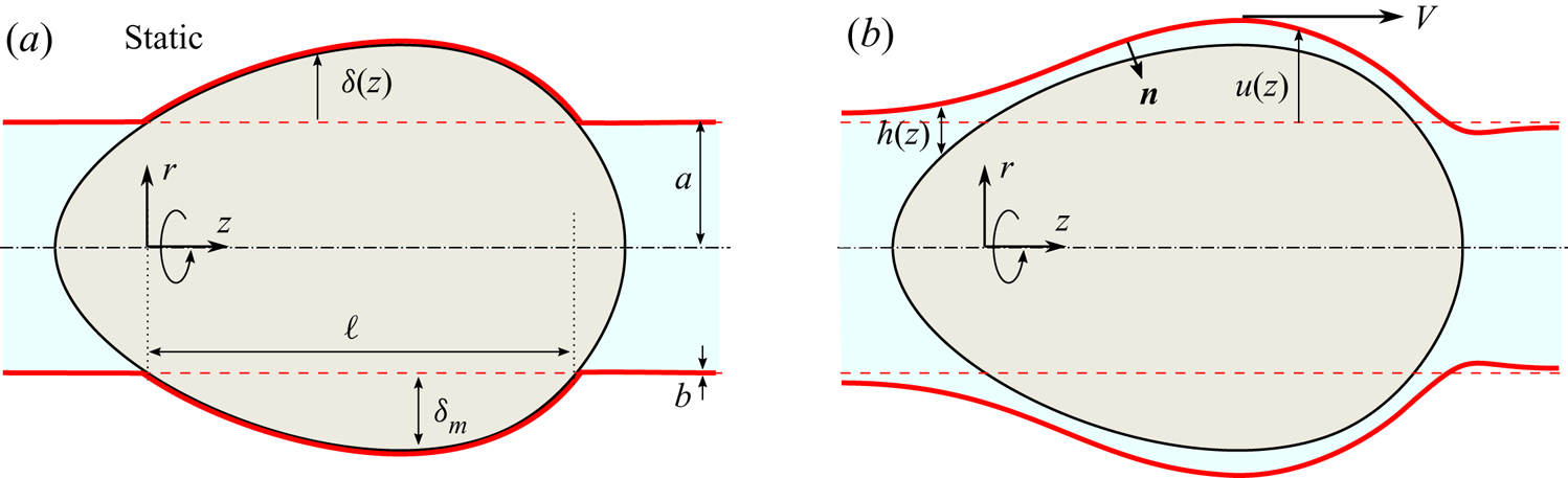
We consider the motion of a rigid axisymmetric intruder through a fluid-filled cylindrical elastic tube, as illustrated in figure 1 for the case that the particle translates from right to left. In its undeformed state, the tube is a cylindrical shell with walls of thickness  $b$ and whose midsurface has a radius
 $a$. The intruding object is wider than the tube and moves through it at a prescribed steady speed
 $V$ as it deforms the tube, due to the application of a force
 $F$ to the left.
Sketch of the cross-section of the set-up showing an axisymmetric intruder translating through an elastic tube (red solid line) filled with liquid, as seen in a reference frame attached to the intruder, which moves from right to left. The radial excess of the intruder beyond the undeformed tube (dashed line) is characterized by  $\delta (z)$ and determines a ‘dry contact’ region of length
 $\ell$, as indicated in panel (a). Relative motion between the intruder and the tube is supported by a fluid film of thickness
 $h(z)$, as shown in panel (b), which is to be determined.

In cylindrical coordinate system  $(r, \theta , z)$ coaxial with the tube (figure 1), the intruder has a radius
 $R(z)$ whose maximum exceeds the tube radius
 $a$. We define the ‘radial excess’ of the intruder relative to the tube by
 $\delta (z) = R(z) - a$ and assume it has a single maximum
 $\delta _m$ (see figure 1); potential consequences of more complex shapes are discussed in § 6. The geometric intersection points of the surfaces of the undeformed (cylindrical) tube surface and that of the intruder define a single contiguous region of length
 $\ell$, where
 $\delta(z)$ is positive (figure 1a). In the absence of motion, and in the limit of negligible bending rigidity, the intruder contacts and deforms the tube in this region, which is the nominal ‘dry’ contact region (Rallabandi et al. Reference Rallabandi, Marthelot, Jambon-Puillet, Brun and Eggers2019). We note that the region of static contact for a finite bending rigidity is generally smaller (by an amount that depends on the wall thickness
 $b$). The motion of the intruder in the presence of a lubricating fluid breaks the solid–solid contact by further deforming the tube and dynamically establishing a fluid film between the intruder and the inner tube surface, as sketched in figure 1(b). Our objective is to calculate the thickness
 $h(z)$ of the lubricating film, and consequently the force necessary to drive the motion of the intruder.
We address the problem using both numerical solutions (using DNS) of the coupled fluid–elastic problem and by developing a reduced-order theory that combines thin-film lubrication with the geometrically nonlinear description of the elastic deformation of the tube. The former is introduced below, while the latter is developed in the § 3.
2.2. Implementation of DNS
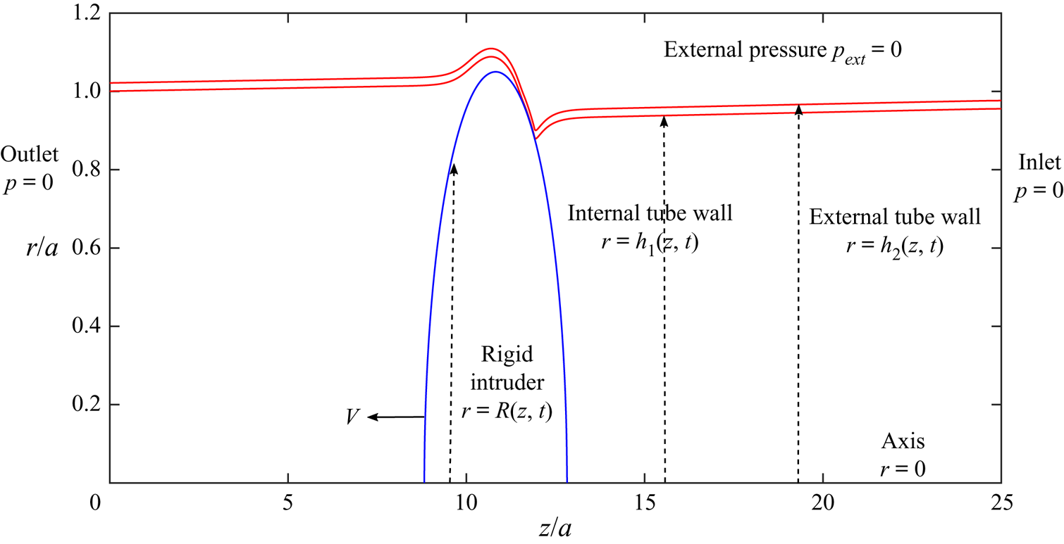
For the full 3-D axisymmetric DNS, we consider a finite tube of length  $L=25 a$ (see figure 2). The reference frame is attached to the left-hand end of the tube while the intruder (blue curve in figure 2), initially at the right-hand end of the tube, moves towards the left-hand end at a constant speed,
 $V$. The problem in this reference system is unsteady and the equations governing the problem are integrated in time until the force required to keep the object moving at constant speed reaches a steady value.
Sketch of the domain and boundary conditions used in the 3-D DNS.

The flow is assumed incompressible and Newtonian (viscosity  $\mu$) and is described by a velocity
 $\boldsymbol {v}(\boldsymbol {x},t)$ and pressure
 $p(\boldsymbol {x},t)$. Neglecting the inertia of the flow and defining the fluid stress tensor
 $\boldsymbol {\sigma }(\boldsymbol {x},t) = - p \boldsymbol {I} + \mu (\boldsymbol {\nabla } \boldsymbol {v} + \boldsymbol {\nabla } \boldsymbol {v}^T)$, the equations of motion of the fluid are
 \begin{equation} \boldsymbol{\nabla} \boldsymbol{\cdot} \boldsymbol{\sigma} = \boldsymbol{0} \quad \text{and} \quad \boldsymbol{\nabla} \boldsymbol{\cdot} \boldsymbol{v} = 0. \end{equation}
The tube is treated as an incompressible 3-D linearly elastic material with Young's modulus  $E$, although we will allow for compressibility of the solid in the theory developed in the next section. The undeformed configuration (stress-free state) of the tube is that of a cylindrical shell with walls of thickness
 $b$ whose inner surface has radius
 $a$. Points in the undeformed state are denoted
 $\boldsymbol {X}$, which are mapped to points in the deformed configuration via
 $\boldsymbol {x} = \boldsymbol {x}(\boldsymbol {X}, t)$. The change in distance between two material points is measured by the deformation tensor
 $\boldsymbol {F} = \partial \boldsymbol {x}/\partial {\boldsymbol {X}}$. Neglecting the inertia of the solid and denoting the solid stress tensor by
 $\boldsymbol {\sigma }_s$, the balance of elastic stresses for an incompressible neo-Hookean solid is (Suo Reference Suo2013; Landau & Lifshitz Reference Landau and Lifshitz1984)
 $$\begin{gather} {\boldsymbol \nabla} \boldsymbol{\cdot} \boldsymbol{\sigma}_s = \boldsymbol{0} \quad \text{where} \ \boldsymbol{\sigma}_s ={-} p_s \boldsymbol{I} + \frac{E}{3} (\boldsymbol{F} \boldsymbol{\cdot} \boldsymbol{F}^T - \boldsymbol{I}), \quad \text{with} \end{gather}$$
 $$\begin{gather}\mathrm{det}\; \boldsymbol{F} = 1. \end{gather}$$
The constraint of incompressibility (2.2b) is enforced by the solid pressure  $p_s(\boldsymbol {x},t)$.
At the inner surface of the tube ( $r = h_1(z,t)$, see figure 2) we apply continuity of fluid and solid velocities and stresses
 \begin{equation} \boldsymbol{v}= \boldsymbol{v}_s,\quad \boldsymbol{n} \boldsymbol{\cdot} \boldsymbol{\sigma} = \boldsymbol{n} \boldsymbol{\cdot} \boldsymbol{\sigma}_s, \quad \text{at}\ r = h_1(z,t), \end{equation}
where  $\boldsymbol {n}$ is the unit normal and
 $\boldsymbol {v}_s = \partial {\boldsymbol {x}(\boldsymbol {X},t)}/\partial {t}$ is the solid velocity. The outer surface of the tube
 $(r = h_2(z,t)$) is stress free,
 \begin{equation} \boldsymbol{n} \boldsymbol{\cdot} \boldsymbol{\sigma}_s = \boldsymbol{0} \quad \text{at}\ r = h_2(z,t). \end{equation}
The no-slip condition is enforced at the surface of the intruder,
 \begin{equation} \boldsymbol{v} ={-} V \boldsymbol{e}_z \quad \text{at}\ r=R_1(z,t), \end{equation}
with regularity conditions  $\partial {v_z}/\partial {r}=v_r=0$ prescribed at the tube axis
 $r = 0$.
At both tube ends,  $z=0$ and
 $z=L$, the pressure is kept zero to avoid the introduction of external pressure gradients
 \begin{equation} p(z=0,r,t)=p(z=L,r,t)=p_{ext}=0. \end{equation}
At these ends, the radial component of velocity is set to zero, and the axial component is computed from the axial momentum equation. At the right-hand end, the tube wall is clamped in the axial direction but it is allowed to move in the radial direction, while at the left-hand end, the tube is free to move in both axial and radial directions. These displacements are accommodated by prescribing zero gradient of tangential stress at the clamped end  $\partial (\boldsymbol {e}_z \boldsymbol {\cdot } \boldsymbol {\sigma }_s) /\partial z|_{z = L}=\boldsymbol {0}$ and zero tangential stress at the free end
 $\boldsymbol {e}_z \boldsymbol {\cdot } \boldsymbol {\sigma }_s|_{z = 0} = \boldsymbol {0}$, the latter corresponding to no stretching of the tube at the left-hand end.
At any time the axial force,  $F(t)$, required to keep the object moving a constant speed
 $V$ is computed by integrating the fluid stresses over the surface of the intruder
 \begin{equation} F (t)=\left. 2{\rm \pi}\int_{z_0}^{z_1} \boldsymbol{n} \boldsymbol{\cdot} \boldsymbol{\sigma} \boldsymbol{\cdot} \boldsymbol{e}_z\, r \sqrt{1 + \left(\mathrm{d}{R}/\mathrm{d}{z} \right)^2} \right|_{r = R(z,t)}\, \mathrm{d} z, \end{equation}
where  $z_0$ and
 $z_1$ are axial positions where the intruder shape meets the axis,
 $R(z_0,t)=R(z_1,t)=0$. As a test of consistency of the results, this force is also computed as the differences of axial elastic force across the ends of the tube
 \begin{equation} F(t)=2{\rm \pi}\left(\int_{r=h_1(L,t)}^{r=h_2(L,t)} \boldsymbol{e}_z \boldsymbol{\cdot} \boldsymbol{\sigma}_s \boldsymbol{\cdot} \boldsymbol{e}_z r \,\mathrm{d} r-\int_{r=h_1(0,t)}^{r=h_2(0,t)} \boldsymbol{e}_z \boldsymbol{\cdot} \boldsymbol{\sigma}_s \boldsymbol{\cdot} \boldsymbol{e}_z r\, \mathrm{d} r\right). \end{equation}
The set of governing equations (2.1a,b)–(2.2) (more precisely, the time-dependent forms of the stress balances but suppressing nonlinear inertia) subject to the boundary conditions (2.3)–(2.6), are integrated simultaneously for the fluid and solid velocities and stresses  $\boldsymbol {v}$,
 $\boldsymbol {\sigma }$,
 $\boldsymbol {v}_s$,
 $\boldsymbol {\sigma }_s$, which depend on both position
 $\boldsymbol {x}$ and time
 $t$. The details of the numerical method are given in Appendix A and follow from the work of Herrada & Montanero (Reference Herrada and Montanero2016) and Snoeijer et al. (Reference Snoeijer, Pandey, Herrada and Eggers2020). In the course of this solution we self-consistently determine the inner and outer surfaces of the tube. The force is monitored over time using both (2.7) and (2.8) (these are verified to be identical for all of the results) until a steady value is attained, which we report simply as
 $F$ in the subsequent sections.
3. Lubrication theory coupled to membrane elasticity
To obtain more insight into the problem, we introduce a simplified description in which we analyse the fluid flow using lubrication theory and describe the tube elasticity using shell theory. It is useful to attach the reference frame to the intruder, so that the tube wall now has a rightward speed  $V$; as a result, we can look for steady solutions directly. In this reference frame we shift the origin of
 $z$ so that the nominal ‘dry’ contact lines are fixed at
 $z =0$ and
 $z = \ell$, identified by geometric intersection of the intruder and the undeformed tube (figure 1). Henceforth, all quantities will be described in this object-attached reference frame, though we retain the same notation
 $z$ as before. The relative motion establishes a thin fluid film of thickness
 $h(z)$, so the local radial deformation of the tube wall is
 $\delta (z) + h(z)$. The shape of the thin film
 $h(z)$ is unknown a priori and must be determined as a part of the solution to the fluid–elastic problem.
We assume that the film is thin relative to the radius of the intruder, and that the intruder has a slender shape, so lubrication theory is applicable. As is typical in lubrication the pressure is constant across the film (Batchelor Reference Batchelor1967) and is related to the axial velocity according to
 \begin{equation} v_z = \frac{1}{2 \mu} \frac{\mathrm{d} p}{\mathrm{d} z} (r - \delta(z)) (r - \left(\delta(z) + h(z)\right)) + V \frac{r - \delta(z)}{h(z)}. \end{equation}
The fluid flux through the film per circumference of the tube is  $q = -h^3/(12 \mu )\, \mathrm {d} p/\mathrm {d} z + V h/2$. At steady state,
 $q$ is a constant and so the pressure must satisfy
 \begin{equation} \frac{\mathrm{d} p}{\mathrm{d} z} = \frac{6 \mu V(h - h^*)}{h^3}, \end{equation}
where we have introduced the constant  $h^* \equiv 2 q/V$, which is the effective gap thickness that can support the flux
 $q$ in axial shear flow between locally cylindrical surfaces; its value is to be determined as part of the solution. We will show that the condition for the lubrication approximation to hold,
 $|\mathrm {d} h/\mathrm {d} z| \ll 1$ reduces to the condition that the intruder has a slender shape (
 $\delta _m/\ell \ll 1$) up to moderately large velocities. For a calculation of the force alone, even this assumption can be dropped in some limits; we will discuss later the self-consistency of our approximations.
We treat the elastic problem based on the elastic shell theory of Sanders (Reference Sanders1963), Koiter (Reference Koiter1966) and Budiansky (Reference Budiansky1968), which we specialize here to axisymmetric deformations of cylindrical shells (i.e. tubes) following Audoly & Pomeau (Reference Audoly and Pomeau2010); see Appendix A of Holmes (Reference Holmes2019) for an overview of nonlinear shell theories. In Rallabandi et al. (Reference Rallabandi, Marthelot, Jambon-Puillet, Brun and Eggers2019), we treat the ‘dry’ version of the present problem, in which the tube is stretched by elastic contacts alone. In the theory, tube walls are assumed thin relative to the radius of its midsurface  $b \ll a$. In particular, we will consider the membrane limit, in which bending rigidity can be neglected.
We describe the elasticity of the tube using a description of its midsurface. Points on the undeformed cylindrical configuration have position  $\boldsymbol {r} = (a, z)$. The tube is deformed by tractions (forces per area)
 $\boldsymbol {f}(z) = \{\,f_r(z), f_z(z)\}$ acting on its surface and line force densities (force per length)
 $\boldsymbol {T}_{\pm \infty }$ acting along its circumference at the two ends, which we take to be at
 $z = \pm \infty$. We define a twistless, axisymmetric deformation field
 $\boldsymbol {u}(z) =(u_r(z), u_z(z))$ that maps material points to their new positions in the deformed state
 $\boldsymbol {r} \mapsto \boldsymbol {r} + \boldsymbol {u}(z)$. Note that this description is an Eulerian one that parameterizes deformations in terms of the axial coordinate
 $z$ of a point in the undeformed state rather than its location
 $z + u_z$ in the deformed state. The distinction between these frames is small when the axial displacement gradient is small, i.e.
 $\mathrm {d} u_z/\mathrm {d} z \ll 1$, which is one of the assumptions of membrane theory. Note that this does not mean that
 $\mathrm {d} u_z/\mathrm {d} z$ can be taken as zero, since the elastic stresses depend linearly on this quantity at leading order.
We denote the membrane strains in the  $z$ and
 $\theta$ directions, respectively, by
 $\varepsilon _{s}$ and
 $\varepsilon _{\theta }$. The membrane strains determine the change in distance between two material points. Assuming small strains and moderate rotations (see Audoly & Pomeau Reference Audoly and Pomeau2010), we can write, for cylindrical tubes,
 \begin{equation} \varepsilon_{s} = u_z' + \tfrac{1}{2}(u_r')^2, \quad \varepsilon_{\theta} = \frac{u_r}{a}, \end{equation}
where the prime denotes the derivative with respect to  $z$. Note that similar geometric approximations for plates (
 $a \to \infty$) form the basis of the Föppl–von Kármán equations (Landau & Lifshitz Reference Landau and Lifshitz1984).
The strain field produces so-called ‘membrane stresses’  $\boldsymbol {N}$ (a vector with units of force per length) with components
 $N_s$ and
 $N_{\theta }$ in the axial and azimuthal directions, respectively. The quantity
 $N_{\theta }(z)$ is called the hoop stress and we refer to
 $N_s(z)$ as the membrane tension, which we denote by
 $T(z)$. For Hookean elasticity, the membrane stresses are given by
 \begin{equation} N_s = T = \frac{E b}{1 - \nu^2} (\varepsilon_{s} + \nu \varepsilon_{\theta} ) \quad \text{and} \quad N_{\theta} = \frac{E b}{1 - \nu^2} (\varepsilon_{\theta} + \nu \varepsilon_{s} ), \end{equation}
where  $E$ is the material's Young's modulus introduced earlier and
 $\nu$ is its Poisson's ratio;
 $\nu = 1/2$ for incompressible materials. We neglect the bending rigidity of the tube, whose contribution to internal stresses scales as
 $b^3$ and is, therefore, small for thin-walled tubes. Introducing the local tangent to the deformed surface by
 $\boldsymbol {t}(z) = (t_r(z), t_z(z))$, local equilibrium of the membrane requires
 $$\begin{gather} \frac{\mathrm{d} }{\mathrm{d} s}( N_s t_r) - \frac{N_{\theta}}{a} + f_r = 0, \end{gather}$$
 $$\begin{gather}\frac{\mathrm{d} }{\mathrm{d} s} (N_s t_z)+ f_z = 0. \end{gather}$$
At the two ends, membrane stresses balance the applied force densities,  $N_s \boldsymbol {t}|_{z = \pm \infty } = \pm \boldsymbol {T}_{\pm \infty }$.
The surface traction on the membrane is related to stresses in the fluid so  ${\boldsymbol {f} = \boldsymbol {n} \boldsymbol {\cdot } \boldsymbol {\sigma }|_{r = a + u_r(z)}}$, where
 $\boldsymbol {n}$ is the fluid-facing normal. For small slopes consistent with lubrication,
 $\boldsymbol {n} \approx -\boldsymbol {e}_{r} + u_r'(z) \boldsymbol {e}_z$ and
 $\boldsymbol {t} \approx u_r'(z) \boldsymbol {e}_{r} + \boldsymbol {e}_z$, and we obtain
 $$\begin{gather} f_r = p(z), \end{gather}$$
 $$\begin{gather}f_z ={-} p u_r'(z) - \left.\mu \frac{\partial v_z}{\partial r}\right|_{r = a + u_r(z)} ={-} p u_r'(z) - p'(z) \frac{h}{2} - \frac{\mu V}{h}, \end{gather}$$
where we have used (3.1). We then eliminate  $\varepsilon _s$ between the two equations of (3.4a,b) and use (3.3a,b) to obtain
 ${N_{\theta } = Eb u_r/a + \nu T}$ (recall that
 $T$ is simply a relabeling of
 $N_s$). Substituting this relation into (3.5) and using (3.6) then yields
 $$\begin{gather} p = \frac{E b}{a^2} u_r + \frac{\nu T}{a} - \frac{\mathrm{d} }{\mathrm{d} z} \left(T \frac{\mathrm{d} u_r}{\mathrm{d} z}\right), \end{gather}$$
 $$\begin{gather}\frac{\mathrm{d} T}{\mathrm{d} z} ={-}f_z = p \frac{\mathrm{d} u_r}{\mathrm{d} z} + \frac{\mathrm{d} p}{\mathrm{d} z} \frac{h}{2} + \frac{\mu V}{h}, \end{gather}$$
where  $h(z) = u_r(z) - \delta (z)$. Equation (3.7a) shows that the pressure in the fluid is balanced by three distinct elastic stress contributions. The first is due to the local radial displacements of the reference state producing a hoop stress, and the second is the additional hoop stress generated by the axial tension for materials with non-zero Poisson's ratio. The third is the normal stress component arising from the tension within the locally rotated (relative to the tube axis) section of the tube. Membrane tension in (3.7b) is generated in response to the tangential stress exerted by the fluid, see (3.6).
The pressure can be eliminated by substituting the  $z$-derivative of (3.7a) into the lubrication relation (3.2), and then using this result for
 $\mathrm {d}{p}/\mathrm {d}{z}$ along with (3.7a) itself in (3.7b). This yields a system of two ordinary differential equations
 $$\begin{gather} \frac{\mathrm{d} u_r}{\mathrm{d} z} + \frac{\nu a}{E b} \frac{\mathrm{d} T}{\mathrm{d} z} - \frac{a^2}{E b}\frac{\mathrm{d}^2}{\mathrm{d}z^2}\left(T \frac{\mathrm{d} u_r}{\mathrm{d} z}\right) - \frac{6 \mu V a^2}{E b} \frac{\left(h - h^*\right)}{h^3}= 0, \end{gather}$$
 $$\begin{gather}\frac{\mathrm{d} T}{\mathrm{d} z} = \frac{E b}{2 a^2}\frac{\mathrm{d} (u_r^2)}{\mathrm{d} z} + \frac{\nu T}{a}\! \frac{\mathrm{d} u_r}{\mathrm{d} z}- \frac{\mathrm{d} }{\mathrm{d} z}\!\left(T \frac{\mathrm{d} u_r}{\mathrm{d} z}\right) \,\frac{\mathrm{d} u_r}{\mathrm{d} z} + \mu V \frac{\left(4 h - 3 h^*\right)}{h^2}, \end{gather}$$
for  $u_r(z)$ and
 $T(z)$. These equations are subject to the condition that the pressure decays away from the intruder and the tube becomes asymptotically flat at both ends,
 $u_r'(\pm \infty ) = 0$ or
 $\boldsymbol {t}(\pm \infty ) = \boldsymbol {e}_z$. Then, the tension on the left-hand end is imposed
 $T(-\infty ) = T_{-\infty }$. The tension
 $T_{\infty }$ on the right-hand end is not directly prescribed but is instead the force (per circumference) required to hold the tube fixed as the intruder slides through it, obtained self-consistently as a solution to the problem. The system (3.8) represents our nonlinear membrane theory, coupled to lubrication equations. It is the basis of our asymptotic description of the small speed limit, and will also be solved numerically for arbitrary speeds, as described in Appendix B.
The force exerted by the fluid on the intruder is the difference of the tensions across the ends of the tube
 \begin{equation} F = 2 {\rm \pi}a \int_{-\infty}^{\infty} f_z \,\mathrm{d} z = 2 {\rm \pi}a (T_{\infty} - T_{-\infty}), \end{equation}
where we have used (3.7b). The equivalence between the force and the difference in tension in (3.9), up to the factor of  $2{\rm \pi} a$, mirrors the equivalence of (2.7) and (2.8). In the particular case of a free left-hand end (
 $T_{-\infty } = 0)$, the tension on the right-hand end
 $T_{\infty }$ is simply the force on the intruder per
 $2 {\rm \pi}a$. Thus, even with a free end, there is always tension to the right of the intruder that is needed to maintain steady-state translation.
We rescale the governing equations (3.8) by focusing on the limit of small velocities. The characteristic radial displacement is set by the maximum radial excess  $\delta _m$ of the object, which sets a characteristic pressure scale
 $E b \delta _m/a^2$ through (3.7a). Using the axial length scale
 $\ell$, the thin-film equation (3.2) therefore yields a film thickness scale
 $\delta _m \lambda ^{1/2}$, where
 \begin{equation} \lambda = \frac{6 \mu V a^2 \ell}{E b \delta_m^3} \end{equation}
is the dimensionless speed of the intruder and has counterparts in the analysis of lubricated Hertzian contacts (Snoeijer et al. Reference Snoeijer, Eggers and Venner2013; Essink et al. Reference Essink, Pandey, Karpitschka, Venner and Snoeijer2021) and plays a role analogous to the capillary number in the seminal work of Bretherton (Reference Bretherton1961). Additionally, the first term of (3.8b) suggests a tension scale  $T_s = Eb \delta _m^2/a^2$. This contribution is produced by
 $p\, \mathrm {d}{u_r}/\mathrm {d}{z}$ (see (3.7b)) and is due to the stretching of the tube over the surface of the oversized intruder. Thus, the tension remains non-zero – in particular over the region of contact with the object – even in the dry (static) limit of vanishingly small speeds (see figure 1). However, its difference across the tube, which yields the drag force per circumference, is identically zero in this limit as expected.
Defining the rescaled variables  $Z = z/\ell$,
 $U = u_r/\delta _m$,
 $\mathcal {T} = T/(Eb\delta _m^2/a^2)$ and
 $H = h/(\delta _m \lambda ^{1/2})$ and introducing the dimensionless parameters
 \begin{equation} \epsilon = \frac{\delta_m}{a} \quad \text{and} \quad k = \frac{a \delta_m}{\ell^2}, \end{equation}
the equations governing the lubrication flow and membrane elasticity (3.8) rescale as
 $$\begin{gather} \frac{\mathrm{d} U}{\mathrm{d} Z} + \nu \epsilon \frac{\mathrm{d} \mathcal{T}}{\mathrm{d} Z} - k \epsilon \frac{\mathrm{d}^2}{\mathrm{d}Z^2}\left(\mathcal{T} \frac{\mathrm{d} U}{\mathrm{d} Z}\right) - \frac{\left(H - H^*\right)}{H^3}= 0, \end{gather}$$
 $$\begin{gather}\frac{\mathrm{d} \mathcal{T}}{\mathrm{d} Z} = \frac{1}{2}\frac{\mathrm{d} (U^2)}{\mathrm{d} Z} + \nu \epsilon \mathcal{T} \frac{\mathrm{d} U}{\mathrm{d} Z}- k \epsilon \frac{\mathrm{d} }{\mathrm{d} Z}\!\left(\mathcal{T} \frac{\mathrm{d} U}{\mathrm{d} Z}\right) \,\frac{\mathrm{d} U}{\mathrm{d} Z} + \lambda^{1/2}\frac{\left(4 H - 3 H^*\right)}{6 H^2}. \end{gather}$$
Here,  $H^* = h^*/(\delta _m \lambda ^{1/2})$ is a dimensionless constant representative of the fluid flux and is to be determined as a part of the solution, see (3.2). Note that
 $U(Z) = \varDelta (Z) + \lambda ^{1/2} H(Z)$, where
 $\varDelta (Z) = \delta (z)/\delta _m$. In Appendix B we describe how to obtain full numerical solutions to the steady-state problem (3.12) with membrane tension for arbitrary speeds
 $\lambda$. The parameter
 $\epsilon$ quantifies the dimensionless radial excess of the intruder and is implicitly small in membrane theory. The parameter
 $k$ depends on the shape of the intruder and is typically
 $O(1)$. We will also define the force scale
 $F_s = 2{\rm \pi} Eb\delta _m^2/a$ and introduce the dimensionless force
 $\mathcal {F} = F/F_s$ given by
 \begin{align} \mathcal{F} &= \int_{-\infty}^{\infty} \left(\frac{1}{2}\frac{\mathrm{d} (U^2)}{\mathrm{d} Z} + \nu \epsilon \mathcal{T} \,\frac{\mathrm{d} U}{\mathrm{d} Z}- k \epsilon \frac{\mathrm{d} }{\mathrm{d} Z}\!\left(\mathcal{T} \frac{\mathrm{d} U}{\mathrm{d} Z}\right) \,\frac{\mathrm{d} U}{\mathrm{d} Z} + \lambda^{1/2}\frac{\left(4 H - 3 H^*\right)}{6 H^2}\right) \,\mathrm{d} Z \end{align}
 \begin{align} &= \mathcal{T}_{\infty} - \mathcal{T}_{-\infty}, \end{align}
which is simply the integral of (3.12b) over the length of the tube.
This completes the set-up of the lubricated membrane theory, which we discuss numerically and theoretically in the following sections. It will turn out to be useful to consider objects with arbitrary shape  $\varDelta (Z)$ including those that are not front-to-back symmetric. At the same time, we note that a broad class of slender intruders that are front-to-back symmetric, including ellipsoids, can be approximated using the parabolic approximation that we detail later in (4.5). This approximation is valid as long as the contacting part of the intruder is slender
 $(\delta _m/\ell \ll 1)$, with the remaining details of the object's shape being captured through the contact length
 $\ell$, its radial excess
 $\epsilon$ and the shape parameter
 $k$, see (3.11a,b). For an ellipsoid with axial half-width
 $R_z$ (and radial half-width
 $a + \delta _m$), the contact length is
 $\ell = 2 R_z \sqrt {1 - (1 + \epsilon )^{-2}}$. Note that the slenderness condition is not a requirement on the overall shape of the object but rather on the contact region. For small
 $\epsilon$, the slenderness condition,
 $\delta _m/\ell = \sqrt {\delta _m a}/(2 \sqrt {2} R_z) \ll 1$, is satisfied as long as
 $\delta _m$ is small and
 $R_z$ is not much smaller than
 $a$.
Below, we will also focus on the situation where the axial stretching of the tube occurs solely due to the motion of the intruder, and where no additional stretch is applied at the ends. This amounts to setting  $\mathcal {T}_{-\infty } = 0$, though in various points in the analysis it will be helpful to retain
 $\mathcal {T}_{-\infty }$ to aid discussion.
Finally, we note that in the lubrication theory we have assumed that the main contribution to the force comes from the neighbourhood of the intruder, and have neglected the resistance coming from the Poiseuille flow far from it. To estimate the contribution from the tube, note that the Poiseuille flow far from the intruder is associated with a volume flux  ${\rm \pi} a^2 V$, which produces a pressure gradient
 $p'(z) = 8\mu V /a^2$. If the total length of the tube is
 $L$, this ‘pure’ Poiseuille flow occurs over a length
 $L - 2 R_z$ of the tube is thus associated with a force
 $F_p \simeq 8{\rm \pi} (L - 2 R_z) \mu V$, where
 $2 R_z$ is the axial width of the intruder. This corresponds to a dimensionless force (in units of the force scale
 $F_s = 2{\rm \pi} Eb\delta _m^2/a$ of lubrication theory) of
 \begin{equation} \mathcal{F}_p \approx \frac{2 \epsilon \lambda (L - 2 R_z)}{3 \ell}. \end{equation}
The force in (3.13) will turn out to scale as  $\sqrt {\lambda }$, while the far-field contribution (3.14) is proportional to the speed
 $\lambda$ itself. The Poiseuille flow contribution is, therefore, small for small speeds
 $(\lambda \ll 1)$ provided that the tube is not too long, a claim that we verify in § 5.
4. The hoop-stress approximation ( $\epsilon = 0$)

Rather than analyse the coupled nonlinear system (3.12) straight away, we first consider a simpler version of the problem that will provide both qualitative and quantitative insights into the solution. This simplification, which can formally be reached by considering the limit  $\epsilon = 0$ of (3.12) while keeping
 $\lambda$ fixed, involves neglecting the influence of the membrane tension on the normal balance of elastic stresses and retaining only hoop stresses, so (3.7a) becomes
 $p(z) \approx E b u_r(z)/a^2$. It will later become apparent that this approximation is a good one to estimate the force on slender intruders, but misses important features downstream of the intruder.
Writing  $U = \varDelta + \lambda ^{1/2} H$, and defining the dimensionless slope of the intruder
 $S(Z) = \mathrm {d}{\varDelta }/\mathrm {d}{Z}$ (by definition
 $O(1)$), (3.12a) reduces to
 \begin{equation} \lambda^{1/2}\frac{\mathrm{d} H}{\mathrm{d} Z} - \frac{\left(H - H^*\right)}{H^3} + S(Z) = 0. \end{equation}
The above equation is subject to the condition  $U(\pm \infty ) = 0$, or
 $H(\pm \infty ) = -\lambda ^{-1/2} \varDelta (\pm \infty )$. Observe that to obtain this approximation, the highest derivative of (3.12) has been dropped and tension no longer affects the fluid flow (this does not, however, mean that the tension itself is zero – see below). The sole dimensionless parameter is
 $\lambda$ and the dependence on
 $k$,
 $\nu$ and
 $\epsilon$ is lost under this approximation. We will later obtain both asymptotic and numerical solutions to (4.1).
Once (4.1) has been solved for  $H(Z)$, it can be used to determine the tension according to
 \begin{equation} \frac{\mathrm{d} \mathcal{T}}{\mathrm{d} Z} = \frac{1}{2}\frac{\mathrm{d} (U^2)}{\mathrm{d} Z} + \lambda^{1/2}\frac{\left(4 H - 3 H^*\right)}{6 H^2}, \end{equation}
which is the analogue of (3.12b). Note that the tension remains finite due to tangential stresses in the fluid despite it not affecting the flow in this  $\epsilon = 0$ approximation. Integrating (4.2) over the entire length of the tube yields the force on the intruder
 \begin{equation} \mathcal{F} = \mathcal{T}_{\infty} - \mathcal{T}_{-\infty} = \lambda^{1/2}\int_{-\infty}^{\infty}\frac{\left(4 H - 3 H^*\right)}{6 H^2} \,\mathrm{d} Z, \end{equation}
where the first term of (4.2) integrates to zero as it is an exact derivative with vanishing  $U$ at both ends of the tube. Solutions to (4.1) and the resulting tension will be presented in more detail after first analysing (4.1) in the limit of small speeds.
4.1. Asymptotic solution for small speeds: $\lambda ^{1/2} \ll 1$

We analyse (4.1) in the limit of small speeds,  $\lambda ^{1/2} \ll 1$, for which the problem splits into three parts. First, the ‘dry’ contact region
 $0 < Z < 1$ along the length of the intruder (the ‘outer’ region in the language of matched asymptotics), and two ‘inner’ regions of width
 $\lambda ^{1/2}$, located around the leftmost contact point
 $Z=0$ (the entry region) and the rightmost point
 $Z=1$ (the exit region), respectively (figure 1).
4.1.1. Thin film contact region (outer solution)
In the outer region ( $0< Z < 1$) the term multiplying
 $\lambda ^{1/2}$ can be neglected in (4.1), so the film thickness
 $H(Z)$ can be found by solving the algebraic equation
 \begin{equation} \frac{H - H^*}{H^3} = S(Z). \end{equation}
If we approximate  $\varDelta$ by a parabola (the ‘parabolic approximation’), and since
 $\varDelta (0) = \varDelta (1) = 0$, as well as the maximum thickness being normalized to unity, we obtain the universal shape
 \begin{equation} \varDelta = 4Z(1-Z) . \end{equation}
As a result, the dimensionless slopes at the entry become  $S_0=4$, and
 $S_1=-4$ at the exit.
Observe that  $H = H^*$ when
 $S = 0$; thus,
 $H^*$ is identified as the film thickness at the maximum radial extent of the intruder. Solutions to the cubic equation (4.4) are of the form
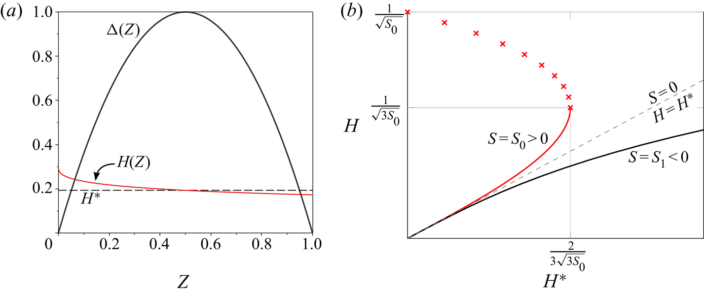
 $H(Z) = f(S(Z); H^*)$, illustrated in figure 3(a). Roots of the cubic equation have to be chosen such that
 $H(Z)$ remains continuous, with
 $H=H^*$ at the maximum, and physically meaningful solutions can only be found for a finite range of combinations of
 $S(Z)$ and
 $H^*$.
(a) The solution  $H(Z)$ of (4.4) for the generic parabolic intruder shape (4.5);
 $H=H^*$ for the maximum of
 $\varDelta$, at
 $Z = 1/2$. (b) The local film thickness
 $H$ as a function of
 $H^*$ for
 $S = S_0 > 0$ (red) and
 $S = S_1 < 0$ (black), as constrained by the outer solution (4.4). The dashed line
 $H = H^*$ corresponds to
 $S = 0$. The space of possible solutions sweeps from the red curve to the black curve across the intruder as the slope changes from
 $S_0$ to
 $S_1$. Continuity with the asymptote
 $H (S \rightarrow 0) \rightarrow H^*$ implies that the upper branch (crosses) is unphysical. Thus, the outer solution restricts
 $H \leq 1/\sqrt {3 S_0}$ and
 $H^* < 2/(3\sqrt {3 S_0})$.

To illustrate this point, it is convenient to think of  $H^*$ as the dependent variable; rearranging (4.4) gives
 \begin{equation} H^* = H (1 - H^2 S), \end{equation}
where we recall that  $H$ and
 $S$ are functions of
 $Z$, but
 $H^*$ is a constant that characterizes the entire solution. As shown in figure 3(b), (4.6) describes two types of curve depending on the sign of
 $S$. At the maximum, the two solutions have to be joined together continuously. For regions where
 $S < 0$,
 $H^*$ grows monotonically with
 $H$, while for any value
 $S > 0$,
 $H^*$ is only positive for
 $H$ in the range
 $0 < H \leq 1/{\sqrt {S}}$, attaining a maximum value of
 $2/(3\sqrt {3S})$ when
 $H = 1/\sqrt {3 S}$. Because
 $H^*$ is a constant, the largest permissible value of
 $H^*$ is set by the maximum positive value of the intruder slope
 $S(Z)$ over the dry contact region. If the intruder shape is convex, this maximum slope occurs at the entrance
 $Z=0$, and we obtain the upper bound (see figure 3)
 \begin{equation} H^* \leq \frac{2}{3 \sqrt{3 S_0}}, \quad \text{where}\ S_0 \equiv S(Z = 0). \end{equation}
This condition must be satisfied for (4.6) to admit solutions throughout the ‘outer’ region  $0< Z<1$.
Furthermore, since the local thickness  $H(Z)$ must approach
 $H^*$ as
 $S(Z) \rightarrow 0$, only the solution branch
 $H < 1/\sqrt {3 S}$ is physically meaningful (figure 3b), leading to the upper bound
 \begin{equation} H(Z) \leq \frac{1}{\sqrt{3 S_0}}. \end{equation}
Thus, for convex intruder shapes the slope at the entry region  $S_0$ limits the space of possible solutions. This conclusion does not involve any detailed analysis of the entry region, but is rather a consequence of the outer problem. We now show that the structure of the entry region picks a unique value of
 $H^*$.
4.1.2. Boundary layers at entrance and exit (inner solutions)
Within the contact region, the film thickness is of order  $h_s=\lambda ^{1/2}\delta _m$ as noted in § 2, while the typical length scale is
 $\ell$, and thus gradients in the film thickness are small in the limit of small
 $\lambda$. However, at the edges of the contact region, located at
 $Z=0$ and
 $Z=1$, the film profile has to adapt to the shape of a tube of constant radius, and axial derivatives in (4.1) can no longer be neglected. In the scaling of (4.1), since
 $S$ and
 $H$ are of order one, balancing the first and the last term we find that boundary layers are of dimensionless size
 $\lambda ^{1/2}$. Since both the film thickness and the width of the boundary layers scale like
 $\lambda ^{1/2}$, the lubrication approximation is not automatically satisfied for small
 $\lambda$. However, within these thin boundary layers,
 $\mathrm {d} h/\mathrm {d} z = O(\delta _m/\ell )$, so the lubrication approximation remains valid for a slender intruder.
We first analyse the boundary layer near the entrance to the film  $(Z = 0)$ which, as we will show, uniquely determines the dimensionless flux
 $H^*$ when combined with (4.4). This feature is analogous to many other similar problems, such as the Bretherton problem for the motion of long bubbles in tubes (Bretherton Reference Bretherton1961), or the motion of an elastic object translating next to an elastic wall (Snoeijer et al. Reference Snoeijer, Eggers and Venner2013). The scaling of the film thickness remains unchanged from the outer problem, so we avoid introducing a new ‘inner’ variable for
 $H$. Rescaling
 $Z = \lambda ^{1/2} \zeta$, we obtain the similarity equation
 \begin{equation} \frac{\mathrm{d} H}{\mathrm{d} \zeta} - \frac{\left(H - H^*\right)}{H^3} + S_0 = 0 + O(\lambda^{1/2}), \end{equation}
since the slope  $S_0 = S(0)$ is approximately constant across the boundary layer.
This equation has to satisfy matching conditions for  $\zeta \rightarrow \pm \infty$: towards the film (
 $\zeta \rightarrow \infty$), where the film thickness is varying slowly,
 $H$ has to match the film thickness of the outer solution, and thus
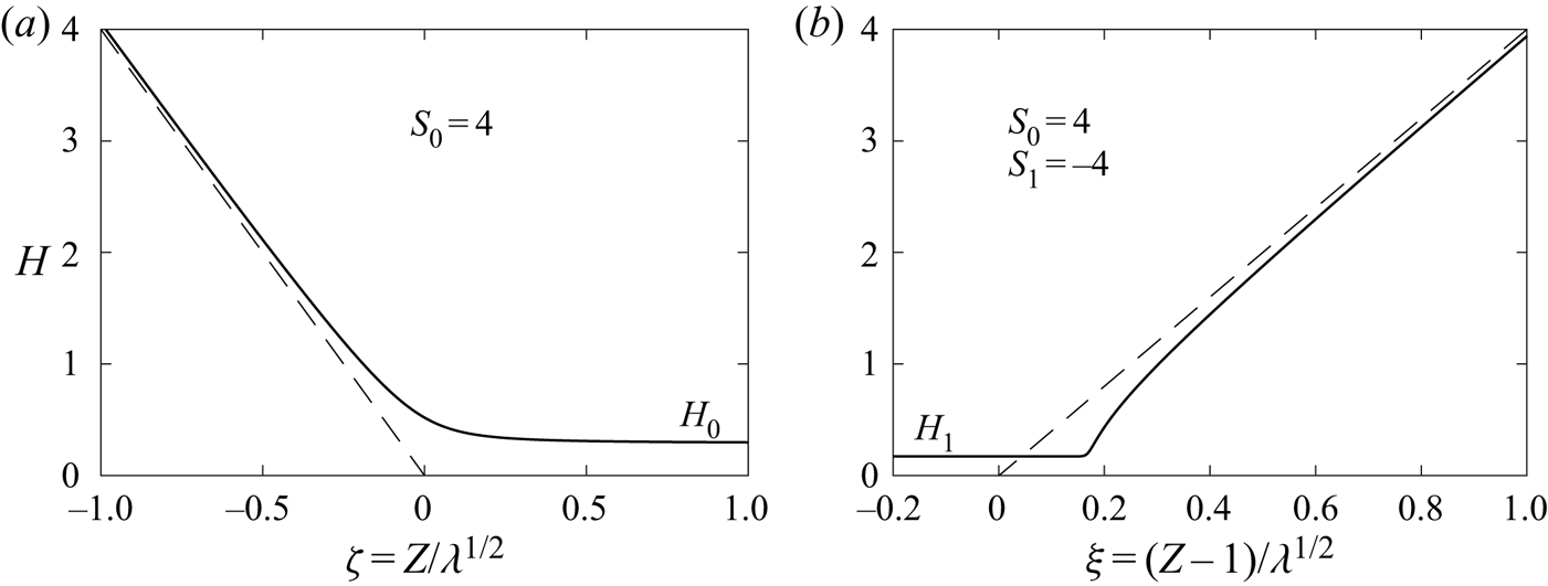
 $H(\zeta \rightarrow \infty ) = H_0 = f(S_0;H^*)$ (cf. Figure 4a). Towards the tube of constant radius, the film thickness increases linearly with the slope of the intruder:
 $H'(\zeta \rightarrow -\infty ) = -S_0$ (figure 4a). This latter condition is satisfied automatically as
 $H$ increases towards
 $\zeta \rightarrow -\infty$, since the second term of (4.9) becomes smaller.
The self-similar profiles (a) at the entry to the film, located at  $Z=0$, and (b) at the back of the film, located at
 $Z=1$, indicated as solid curves. Towards the left and right in panels (a,b), respectively, the profiles asymptote to the undeformed tube, represented by the dashed lines. The dimensionless slopes are those of the parabolic approximation (4.5).

We now show that the condition as  $\zeta \rightarrow \infty$ selects a unique solution to (4.9): substituting
 $H(\zeta ) \approx H_0 + G(\zeta )$ into (4.9) and linearizing in
 $G$ we find
 \begin{equation} \frac{\mathrm{d} G}{\mathrm{d} \zeta} = \frac{1}{H_0}\left(\frac{1}{H_0^2} -3 S_0\right) G \implies G(\zeta) \propto \exp\left\{\frac{1}{H_0} \left(\frac{1}{H_0^2} -3 S_0\right) \zeta\right\}. \end{equation}
For the perturbation  $G(\zeta )$ to remain small as
 $\zeta \gg 1$ requires that
 $H_0 \geq 1/\sqrt {3 S_0}.$ This condition is consistent with the previously obtained upper bound (4.8) only when
 \begin{equation} H_0 = \frac{1}{\sqrt{3 S_0}}, \end{equation}
which sets the film thickness at the entrance. Using (4.4) we obtain
 \begin{equation} H^* = \frac{2}{3 \sqrt{3 S_0}}, \end{equation}
which shows that the boundary layer solution selects the largest possible flux  $H^*$ that permits solutions of the outer problem (4.4). Separating variables, and using (4.12), (4.9) can be solved as
 \begin{align} \zeta &={-}S_0^{{-}3/2}\int^{S_0^{1/2}H}\frac{G^3\, \mathrm{d} G} {\left(G + 2/\sqrt{3}\right) \left(G - 1/\sqrt{3}\right)^2} \end{align}
 \begin{align} &={-}\frac{H}{S_0} + \frac{1}{9 S_0^{2}\left(H - H_0\right)} + \frac{8 }{9\sqrt{3} S_0^{3/2}} \ln\left(\frac{H+2H_0}{H-H_0}\right), \end{align}
which contains  $S_0$ as the sole parameter. The constant of integration has been chosen such that
 $H = -S_0\zeta + O(1/\zeta )$ for
 $\zeta \rightarrow -\infty$, which is the profile of the undeformed tube. This function is plotted in figure 4(a). Clearly, (4.13a) has the required linear growth for
 $\zeta \rightarrow -\infty$ (first term on the right-hand side). On the other hand, as
 $H$ approaches
 $H_0$ for
 $\zeta \rightarrow \infty$, the second term on the right-hand side of (4.13a) dominates, and the profile approaches its limiting thickness as a power law
 $H \sim H_0 + 1/({9 S_0^2\zeta })$.
A boundary layer of size  $\lambda ^{1/2}$ also exists near the exit
 $Z= 1$, where we denote the slope as
 $S_1 = S(Z=1) < 0$. However,
 $H^*$ is now fixed, having been selected at the entrance as usual (see also Bretherton (Reference Bretherton1961) and Snoeijer et al. (Reference Snoeijer, Eggers and Venner2013)). Introducing the similarity variable
 $\xi = (Z - 1)/\lambda ^{1/2}$ at the exit, (4.9) remains the same (with the substitution
 $S_0 \mapsto S_1$), but the matching conditions are reversed:
 $H(\xi \rightarrow -\infty ) = H_1 = f(S_1;H^*)$ toward a film on the left, and
 $H'(\xi \rightarrow \infty ) = S_1$ toward the tube on the right. Linearizing around a constant film thickness
 $H_1$ as before, we find
 \begin{equation} H(\zeta) = H_1 + A \exp\left\{ \frac{1}{H_1} \left(\frac{1}{H_1^2} - 3 S_1 \right) \xi\right\} , \quad \text{as}\ \xi \rightarrow - \infty. \end{equation}
Now the prefactor in the exponential is always positive, so for  $\xi \rightarrow -\infty$ the solution converges exponentially onto the correct boundary condition (the outer problem), as seen in figure 4(b), regardless of
 $H^*$. The solution near the exit is given by
 \begin{equation} \xi = \int^{H}\frac{G^3 \,\mathrm{d} G}{G-H^*-S_1 G^3} , \end{equation}
subject to  $H = -S_1\zeta + O(1/\zeta )$ for
 $\zeta \rightarrow \infty$, which we calculate numerically (figure 4b). The result now depends on the intruder shape at both the entrance and the exit through the values of
 $S_0$ and
 $S_1$ separately. As before, numerical solutions of (4.1) near the exit collapse onto the asymptotic solution (4.15) for small
 $\lambda$. It will turn out that the entry region remains nearly unchanged in the fully coupled problem (3.12), while the exit region is modified quantitatively by membrane tension.
4.1.3. Force on the intruder and tension in the tube
The force on the intruder is obtained by evaluating the integral in (4.3). This calculation simplifies for  $\lambda ^{1/2} \ll 1$ since its main contribution comes from the thin film ‘contact’ region
 $0< Z<1$, with the contribution from boundary layers being
 $O(\lambda ^{1/2})$ smaller. Thus, we can approximate
 \begin{equation} \mathcal{F} = \lambda^{1/2}\int_{0}^{1} \frac{4 H - 3 H^*}{6 H^2} \,\mathrm{d} Z + O(\lambda). \end{equation}
Within the limits of the above integral,  $H(Z)$ is obtained by solving the cubic equation (4.4), where
 $S(Z)$ is given by the shape of the intruder. Note that at low speeds contributions to the force only come from the contact region, where the lubrication approximation is valid even without assuming a slender intruder.
Equation (4.16) must be integrated numerically in general, though for the parabolic approximation (4.5) (so  $S_0 = 4$) the integral can be evaluated analytically by transforming to
 $H$ as the integration variable, to give
 $\mathcal {F} \simeq 0.873 \lambda ^{1/2}$. For a more general shape, a convenient approximation for
 $\mathcal {F}$ is obtained by observing that near the middle of the thin film (where
 $S$ is small),
 $H \approx H^*$ (the profile
 $H(Z)$ is approximated by the dashed line in figure 3a). With this approximation, the integral (4.16) becomes trivial, and using (4.12), results in
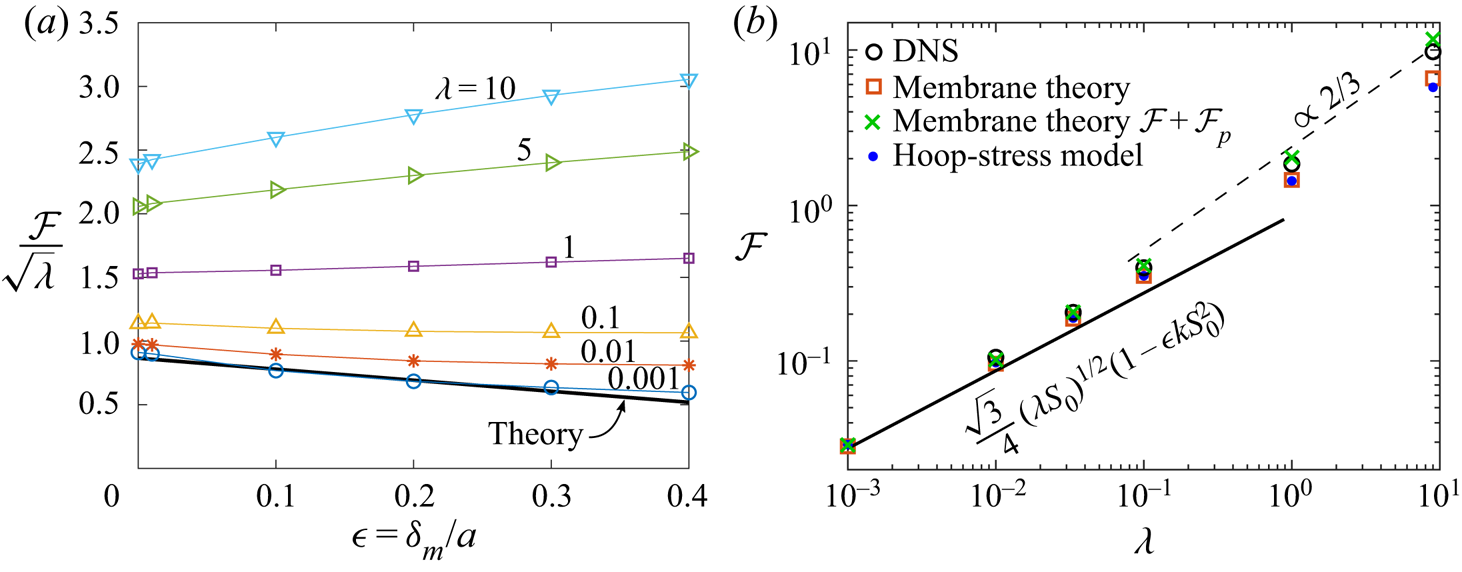
 \begin{equation} \mathcal{F} \simeq \frac{\sqrt{3}}{4}(\lambda S_0)^{1/2} \ \text{for}\ \lambda^{1/2} \ll 1. \end{equation}
For the parabolic intruder, this approximation yields  $\mathcal {F} \simeq 0.866 \lambda ^{1/2}$, which is remarkably close to the exact result (
 $\approx 0.8\,\%$ error). This surprisingly simple expression (4.17) predicts that the dimensionless force depends solely on the slope of the intruder surface at the entrance region. The dependence of
 $\mathcal {F}$ on local slope
 $S_0$ at the entry despite shear stresses being significant over the entire contact region (
 $0 < Z < 1$) is due to the fact that the entrance selects the fluid flux
 $H^* \propto S_0^{-1/2}$ through the film, see (4.12). Later we will show that the simple approximation (4.17) is robust to changes in intruder shape as long as it remains slender.
4.2. Comparison with numerical solutions of the lubricated hoop-stress model
We will now evaluate the quality of our approximations against numerical solutions of the lubrication description, as given by (4.1). To this end we integrate (4.1) from the right with a guess for  $H^*$, which is adjusted until boundary conditions are satisfied to the far left of the intruder.
4.2.1. Symmetric intruders
We first focus on the generic slender axisymmetric intruder ( $\delta _m/\ell \ll 1$), which is also fore-and-aft symmetric (e.g. a prolate ellipsoid) and can be approximated by the quadratic function (4.5) with
 $S_0 = \varDelta '(0) = 4$. For an ellipsoid of axial half-width
 $R_z$ (the half-width in the radial direction is
 $a + \delta _m$), the dry contact length is
 $\ell \simeq 2 \sqrt {2R_z^2 \delta _m/a}$ in the limit
 $\delta _m \ll a$.
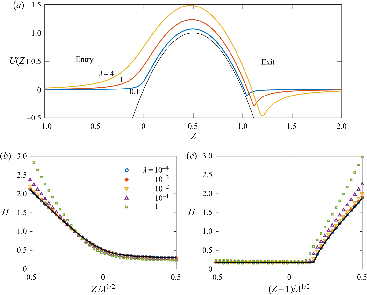
Figure 5(a) shows numerical results of lubrication theory (4.1) for the normalized radial displacement of the tube  $U(Z) = u_r(z)/\delta _m = \varDelta (Z) + \lambda ^{1/2} H(Z)$ for this shape. The tube deformation relaxes over a length scale that increases with increasing
 $\lambda$ corresponding, for example, to faster translation speeds or softer tubes. As
 $\lambda \rightarrow 0$, the solution adopts a boundary-layer structure with a dimensional axial width
 $\lambda ^{1/2} \ell$, as expected from § 4.1. Solutions for the film near the entrance
 $(Z = 0)$ and exit
 $(Z = 1)$ regions are shown as functions of the rescaled boundary layer coordinates in figure 5(b) and figure 5(c), respectively. Numerical solutions are found to collapse onto the theoretical predictions (4.13a) and (4.15) for the entry and exit regions for values of
 $\lambda \lesssim 1$. The qualitative structure of the entry and exit layers remains unchanged even when
 $\lambda \gtrsim 1$.
The film shape for an intruder with parabolic shape (4.5) within the hoop stress approximation. The object translates leftward relative to the tube. (a) Numerical results from solving (4.1) for the normalized radial displacement  $U(Z)$ of the tube. The tube deformation relaxes over a length scale that increases with
 $\lambda$. (b,c) Profiles of film thickness
 $H$ in the boundary layers near the entry region (b) and exit region (c), where numerical solutions (symbols) and theory (solid lines) are shown. Observe that the film thickness in the dry contact region
 $0< Z<1$ is relatively insensitive to
 $\lambda$.

We now test the dependence of the solution on  $\lambda$ more systematically, and over a very wide range. We will see below that even in the limit
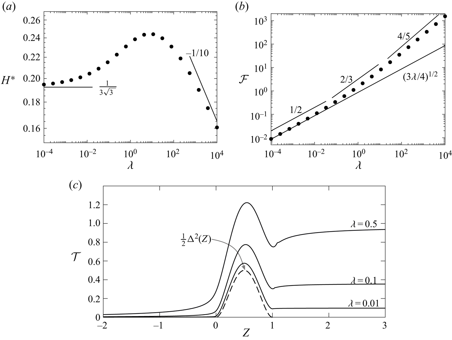
 $\lambda \gg 1$ lubrication theory can be used to calculate the force. As seen in figure 6(a), the dimensionless fluid film thickness
 $H^*$ (thickness at the maximum of the intruder), is relatively insensitive to
 $\lambda$, even over several orders of magnitude. The asymptotic result
 $H^* = 1/{(3 \sqrt {3})}$ from (4.12) for
 $\lambda \ll 1$ (note that
 $S_0 = \varDelta '(0) = 4$ for the chosen intruder shape) is indicated by the horizontal line.
Numerical results from solving (4.1). (a) Rescaled flux  $H^*$ versus
 $\lambda$ for the generic symmetric intruder (4.5), showing the asymptotic behaviour
 $H^* = 1/{(3 \sqrt {3})}$ at small
 $\lambda$ (solid line) and the scaling behaviour
 $H^* \propto \lambda ^{-1/10}$ at large
 $\lambda$. (b) Rescaled force
 $\mathcal {F}$ as a function of
 $\lambda$, showing the small-
 $\lambda$ asymptotic results (4.17) (solid line) and the scaling laws
 $\mathcal {F} \propto \lambda ^{2/3}$ and
 $\mathcal {F} \propto \lambda ^{4/5}$ for intermediate and large
 $\lambda$, respectively. (c) Dimensionless tension
 $\mathcal {T}(Z)$ for different values of
 $\lambda$. The limiting value for
 $Z \to \infty$ is the dimensionless force
 $\mathcal {F}$. The dashed line is
 $\varDelta ^2/2$ and corresponds to the tension over the intruder in the dry limit
 $\lambda \to 0$.

When  $\lambda \gg 1$, both the axial length scale and the film thickness become much greater than the geometric scales imposed by the intruder, a trend which is already apparent in figure 5(a). At large axial distances from a paraboloidal intruder the surface slope grows as
 $S(Z) = \varDelta '(Z) \sim 4Z$. Requiring a balance of all three terms of (4.1) far away from the intruder reveals a film thickness
 $H = O(\lambda ^{-1/10})$ with variations over a characteristic axial scale
 $Z = O(\lambda ^{1/5})$ (i.e.
 $h = O(\delta _m \lambda ^{2/5})$,
 $z = O(\ell \lambda ^{1/5})$). This scaling law for
 $H$ is reflected in the behaviour of
 $H^*$ for
 $\lambda \gtrsim 10^2$, indicated in figure 6(a). Note that in this limit
 $\mathrm {d} h/\mathrm {d} {z} = O(\lambda ^{1/5}\delta _m/ \ell )$, which is assumed small in the theory, so the intruder must be sufficiently slender for the thin-film and the hoop-stress approximations to remain valid at large
 $\lambda$. Note also that the paraboloidal approximation of the surface shape is valid over axial length scales
 $Z \lesssim R_z/\ell$, so the above scaling relations for large
 $\lambda$ are valid if
 $\lambda ^{1/5} \lesssim R_z/\ell$.
Using (4.17), the dimensionless force on the generic symmetric intruder is approximately
 \begin{equation} \mathcal{F} \simeq \left(3 \lambda/4\right)^{1/2} \quad \text{or} \quad F \simeq 6 {\rm \pi}\left( \mu V E b\right)^{1/2} (2R_z^2 \delta_m^3/a)^{1/4} , \quad \text{for}\ \lambda \ll 1. \end{equation}
Figure 6(b) shows numerical results (symbols) for the dimensionless force on the intruder, with the prediction of (4.18) indicated as a solid line, showing good agreement for  $\lambda \lesssim 0.1$.
At intermediate  $\lambda \gtrsim 1$, the axial length is still set by the intruder geometry, while the film thickness becomes comparable to
 $\delta _{m}$ (recall that the characteristic film thickness is
 $h_s = \lambda ^{1/2} \delta _m$). A balance between the first two terms in (4.1) with
 $Z = O(1)$ determines
 $H = O(\lambda ^{-1/6})$. Then, the force integral (4.3) yields the scaling estimate
 \begin{equation} \mathcal{F} \propto \lambda^{2/3} \quad \text{or} \quad F \propto (E b \delta_m R_z^2)^{1/3} (\mu V)^{2/3} , \quad \text{for}\ \lambda \gtrsim 1. \end{equation}
This approximate scaling law at intermediate  $\lambda$ is indicated in figure 6(b), and accurately represents the numerical results in the range
 $0.1 \lesssim \lambda \lesssim 10$.
For  $\lambda \gg 1$, the characteristic scales
 $Z = O(\lambda ^{1/2})$ and
 $H = O(\lambda ^{-1/10})$, obtained earlier, yield the scaling law
 \begin{equation} \mathcal{F} \propto \lambda^{4/5} \quad \text{or} \quad F \propto (\mu V)^{4/5} (E b R_z^4 a)^{1/5}, \quad \text{for}\ \lambda \gg 1, \end{equation}
when substituted into (3.13). This prediction is consistent with numerical calculations for  $\lambda \gtrsim 10^2$, as indicated in figure 6(b). Since the force grows sublinearly in (4.20), this is subdominant to the contribution (3.14) coming from the pipe, in the limit of large
 $\lambda$. Whether the contribution to the force (3.14) from the Poiseuille flow can in fact be neglected has to be checked in the individual cases. The forgoing results are summarized in table 1.
Summary of scaling laws in different ranges of  $\lambda$ (see (4.1)) for a generic fore-and-aft-symmetric intruder with axial curvature
 $1/R_z$ and a maximum radius
 $a + \delta _{m}$. The shape of such an intruder is
 $\varDelta (Z) = 4 Z (1- Z)$. The results are valid for
 $\delta _{m} \ll \ell$, where
 $\ell = 2\sqrt {2 \delta _{m} R_z^2/a\,}$. Prefactors for
 $\lambda \ll 1$ are provided by the asymptotic theory.

The membrane tension profiles  $\mathcal {T}(Z)$, obtained by integrating (4.2) subject to the stress-free condition at the left-hand end (
 $\mathcal {T}_{-\infty } = 0$), are shown in figure 6(c) for a few different
 $\lambda$. In the laboratory frame, the intruder moves leftward and the tube is fixed at the right-hand end, so the tension approaches zero on the left-hand end of the tube (which is stress free) and approaches a finite value
 $T_{\infty }$ on the right-hand end. This is made clear in the limit
 $\lambda ^{1/2} \ll 1$, where
 $\mathcal {T}(Z<0) \sim \mathcal {T}_{-\infty } = 0$ due to the small
 $U$ and large
 $H$. Over the contact region, where
 $U(Z) \approx \varDelta (Z)$, we find
 $\mathcal {T} = \varDelta ^2(Z)/2 + O(\lambda ^{1/2})$, which is the only part of the tension that survives in the static dry limit. To the right, however, the tension approaches the drag force on the intruder, having ‘picked up’ the shear stress over the thin-film contact region, so
 $\mathcal {T}(Z > 0) \sim \mathcal {T}_{\infty } = \mathcal {F} \simeq ({\sqrt {3}}/{4})(\lambda S_0)^{1/2}$. The transition between
 $T \sim \varDelta ^2/2$ over the film and
 $T \sim T_{\infty }$ on the right of the object occurs through the boundary layer at the film's exit. This distribution of tension will remain qualitatively intact for the full membrane theory (3.12). Observe that the shear stress, which is the derivative of the tension, is restricted to
 $0< Z<1$ for
 $\lambda ^{1/2}$, consistent with the approximation (4.16).
The necessary condition for the thin-film approximation  $(\mathrm {d} h/\mathrm {d} z \ll 1)$ to apply is that the intruder is slender:
 $\delta _m \ll \ell$ for moderate
 $\lambda$, and the slightly stricter condition
 $\lambda ^{1/5} \delta _m \ll \ell$ for
 $\lambda \gtrsim 10^2$. For small
 $\lambda$,
 $\mathrm {d} h/\mathrm {d} z$ scales as
 $\lambda ^{1/2}\delta _m/\ell$ in the outer region and as
 $\delta _m/\ell$ in the entry and exit regions. This means that the present thin-film analysis of the outer problem for
 $\lambda ^{1/2} \ll 1$ remains valid even for non-slender intruders even though this approximation is inadequate in the entry and exit regions. Because the force is dominated by the outer problem (see § 4.1.3), we speculate that
 $\mathcal {F} \propto \lambda ^{1/2}$ may persist for non-slender intruders at small
 $\lambda$, although the modified flow in the entry region may select a different
 $H^*$ and, therefore, a different prefactor for
 $\mathcal {F}$. We note the subinear power-law dependence of the force on the velocity is qualitatively similar to the experimental results of Tani et al. (Reference Tani, Cambau, Bico and Reyssat2017).
4.3. Effect of intruder shape
We now consider slender intruders of arbitrary (but still axisymmetric) shape, still within the hoop-stress-only approximation (4.1). The force on a slender intruder, according to (4.17) (neglecting the influence of tension), is
 \begin{equation} \mathcal{F} \simeq \frac{\sqrt{3}}{4} (S_0 \lambda)^{1/2} \quad \text{or} \quad F \simeq \frac{3 \sqrt{2}}{2} {\rm \pi}\left(E b \mu V\right)^{1/2} \ell\left. \left(\frac{\mathrm{d} \delta}{\mathrm{d} z}\right)^{1/2} \right|_{z = 0}. \end{equation}
Compared with the preceding subsection, we will no longer assume a parabolic shape, which implies  $S_0=4$. Instead,
 $S_0$ is now a free parameter. The result (4.21) predicts a particularly simple dependence of the force on the intruder's shape. For example, one might ask which orientation of an egg travelling down an oviduct (Bradfield Reference Bradfield1951) might offer the least resistance? Equation (4.17) clearly favours a small value of
 $S_0$, which occurs if the intruder enters with its narrow (i.e. more gently inclined) side first.
We will now test these predictions using our numerical simulations of the lubrication equations (4.1) by introducing a family of intruder shapes whose degree of asymmetry can be varied systematically. For simplicity, we use piecewise functions
 \begin{equation} \varDelta(Z) = g(Z;Z_m) \equiv \left\{ \begin{array}{@{}ll} 1 - \left(\dfrac{Z - Z_m}{-Z_m}\right)^2, & Z \leq Z_ m,\\ 1 - \left(\dfrac{Z - Z_m}{1-Z_m}\right)^2, & Z > Z_m, \end{array}\right. \end{equation}
parameterized by  $0 < Z_m < 1$. Defined this way,
 $\varDelta (Z)$ is convex with a maximum value of unity at
 $Z = Z_m$, and is continuous in value and slope throughout. For
 $Z_m=1/2$ one obtains the previous parabolic shape, whereas shapes with
 $Z_m<1/2$ are wider on the left, which is the part that goes first. Conversely, shapes with
 $Z_m>1/2$ are increasingly narrow toward the leading edge. Slopes at the entry and exit are
 $S_0 = 2/Z_m$ and
 $S_1 = -2/(1-Z_m)$, respectively.
We vary  $Z_m$ between
 $0$ and
 $1$ to smoothly change the shape of the intruder and, consequently, the slope
 $S_0$. We solve the problem numerically for
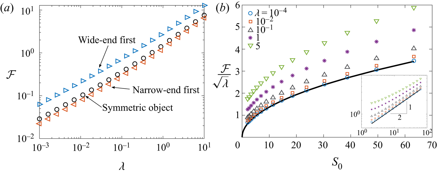
 $H(Z)$ and then compute the force on the intruder using (3.13). Figure 7(a) shows that the force is indeed smaller for intruders with smaller slope
 $S_0$ at the entrance of the thin film contact region, as predicted by (4.17). This qualitative prediction remains valid over the entire range of
 $\lambda$. Thus, asymmetric intruders travelling narrow-end-first encounter a lower resistance than the same object travelling wide-end first. This fore-and-aft symmetry breaking of the mobility of the object in spite of negligible inertia is a result of nonlinearities due to the coupling between the fluid flow and the tube deformation.
(a) Dimensionless force  $\mathcal {F}$ versus
 $\lambda$ for objects of different shapes defined by (4.22). The drag force for narrow-end-first motion (here,
 $Z_m = 0.9$) is least, followed by a symmetric object (
 $Z_m = 0.5$) and then wide-end-first motion has the highest drag (here,
 $Z_m = 0.1$). Note that the two asymmetric cases correspond to the same physical intruder, but with their orientations flipped relative to the direction of motion. (b) Rescaled force
 $\mathcal {F}/\lambda ^{1/2}$ versus the slope at the entry region
 $S_0 = S(Z = 0)$ for different values of
 $\lambda$ for intruders prescribed by (4.22). The solid line is the prediction of (4.21),
 $\mathcal {F} \simeq (3\lambda S_0/16)^{1/2}$. The inset plots the same data on a logarithmic scale, showing that the scaling relation
 $\mathcal {F} \propto S_0^{1/2}$ holds approximately even when
 $\lambda = O(1)$. All results have been obtained from a numerical solution of the lubrication equations (4.1).

To test the dependence of  $\mathcal {F}$ on
 $S_0$, we vary the shape of the intruder through the parameter
 $Z_m$ at fixed
 $\lambda$. Figure 7(b) shows the force as a function of the entry slope
 $S_0$ of the intruder. Symbols represent numerical results of the hoop-stress (
 $\epsilon = 0$) model, while the solid curve is the prediction of (4.17) valid for small
 $\lambda$. The force increases relative to this asymptotic prediction at larger
 $\lambda$, but the scaling
 $\mathcal {F} \propto S_0^{1/2}$ appears to be relatively robust over a wide range of
 $\lambda$ (inset of figure 7b).
5. Results of membrane theory and comparison with DNS
Equipped with physical and mathematical insight into the solution structure and the force from the preceding analysis, we will now address the full problem (3.12) coupling nonlinear membrane elasticity with lubrication theory, in which tension enters both the normal and tangential stress balances. We will see that the finite tension produces a qualitative modification to the shape of the thin film relative to the hoop-stress approximation of the previous section. The tension also produces a correction to the propulsion force (4.17), to leading order in the radial deformation  $\epsilon$.
To solve (3.12) and compare the results with DNS, we set  $\mathcal {T}_{-\infty } = 0$ (the left-hand end of the tube is force free), so that
 $\mathcal {T}_{\infty }$ is the force that must be exerted to move the object. We solve the system of governing equations (3.12) numerically for the dimensionless pressure
 $P$, displacement
 $U$ and tension
 $\mathcal {T}$ using a relaxation procedure; details are outlined in Appendix B. To compare the predictions of membrane theory with the simulations, we focus on ellipsoidal intruders with axial half-width
 $R_z = 2a$ and with a radial excess
 $\epsilon = \delta _m/a = 0.05$. The walls of the tube in the simulations have thickness
 $b = 0.001 a$ so that the bending rigidity of the tube is small.
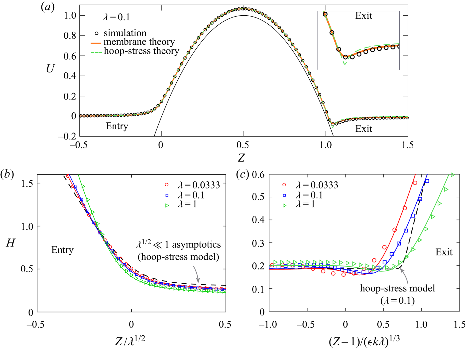
Figure 8 shows the comparison between membrane theory and DNS of the dimensionless tube shape  $U(Z)$ and the film thickness profiles
 $H(Z)$ for this configuration with different values of the dimensionless speed
 $\lambda$. In figure 8(a), for
 $\lambda = 0.1$, we see that the membrane theory accurately reproduces the DNS for the deformation of the tube
 $U(Z)$. Also shown is the hoop-stress-only theory, which does surprisingly well at the entry and over the contact region, but deviates at the exit. In particular, the tube displacement approaches a finite negative value to the right of the intruder in the membrane theory and DNS, while the hoop-stress model predicts a vanishing tube displacement, after a sharper change of curvature around
 $Z = 1$ (inset of figure 8a).
Tube displacement and film thickness profiles for an ellipsoid ( $R_z = 2 a$,
 $\epsilon = 0.05$,
 $b = 0.001 a$) showing good agreement between DNS (described in § 2, markers) and solutions of the nonlinear membrane theory (solid curves). (a) Radial displacement of the tube for
 $\lambda = 0.1$ with the prediction of the hoop-stress-only theory indicated as a dashed curve. The hoop-stress-only theory is a good approximation except for near the exit to the film
 $Z > 1$, where the membrane theory remains in excellent agreement with DNS. (b) Film thickness profile versus the entry layer coordinate
 $Z/\sqrt {\lambda }$, showing excellent agreement between DNS and membrane theory. The
 $\lambda ^{1/2} \ll 1$ asymptotic solution of the hoop-stress theory at the entry (4.13a) is indicated as a dashed curve. (c) Film thickness profile near the rear of the intruder obtained from DNS and membrane theory, showing oscillations over a characteristic dimensional axial scale
 $\ell (\epsilon k \lambda )^{1/3}$. This axial scale and the oscillations of film profile are absent in the hoop-stress theory, which is indicated by the dashed line for
 $\lambda = 0.1$.

At the entrance to the film the structure and  $\lambda ^{1/2}$ axial scaling of the entrance
 $(Z = 0)$ discussed in the previous section persist. The results from both simulations and membrane theory near
 $Z = 0$ collapse when plotted against the rescaled boundary layer coordinate
 $Z/\sqrt {\lambda }$, as discussed in § 5. These results are also well described by the hoop-stress approximation at the front (4.13a); as we will later show, a finite tension only produces only a small correction at the film's entrance.
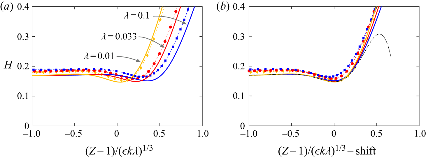
The notable feature that is qualitatively different is the film thickness at the back of the intruder  $(Z = 1)$, which now shows oscillations. These oscillations are absent from the hoop-stress model and are a consequence of finite tension (finite
 $\epsilon$) in the normal balance of stress. Figure 8(c) emphasizes these features by plotting the film thickness versus a new boundary layer coordinate
 $(Z- 1)/(\epsilon k \lambda )^{1/3}$. The membrane theory again captures these features of the DNS, whereas the hoop-stress model presents a qualitatively different picture (monotonic growth of
 $H$ over an axial scale
 $\lambda ^{1/2}$). The new boundary layer scale
 $(\epsilon k \lambda )^{1/3}$ can be rationalized by balancing the fluid pressure with the highest derivative in (3.8a), which involves a membrane tension
 $\mathcal {T} = O(\lambda ^{1/2})$. This scaling and the resulting oscillatory structure at the back will be analysed in detail later in the next section.
5.1. Membrane theory for small speeds: $\lambda ^{1/2} \ll 1$

Having established the accuracy of the membrane theory relative to the DNS, we now analyse it in the limit of small speeds:  $\lambda ^{1/2} \ll 1$. The tension profiles
 $\mathcal {T}(Z)$ will turn out to be qualitatively similar to the hoop-stress results shown in figure 3(c). We again separate inner and outer problems. Outer problems occur over the dry contact region (
 $0 < Z < 1$) as before, as well as over the non-contacting regions
 $(Z < 0)$ and
 $(Z > 1)$, which are now non-trivial owing to a finite tension. As before, the inner problems resolve boundary layers at the entry
 $(Z = 0)$ and exit
 $(Z = 1)$ regions and are necessary to match between outer problems. There are two contact points, one at
 $Z = 0$ and another at
 $Z = 1$, where the non-contacting and contacting regions of the solution meet. We discuss how these features are modified and inform the solution for small non-zero
 $\lambda$.
We analyse the governing equations of the full lubricated membrane theory (3.12) by first considering the contact region  $(0 < Z < 1)$ where
 $\varDelta = O(1)$ and
 $H = O(1)$, so
 $U \sim \varDelta$. Collecting terms of order
 $\lambda ^0$, one obtains
 $$\begin{gather} \frac{H - H^*}{H^3}= \varDelta' + \epsilon \nu \mathcal{T}' - \epsilon k (\mathcal{T} \varDelta')'', \end{gather}$$
 $$\begin{gather}\mathcal{T}' = \varDelta\varDelta' + \nu \epsilon \mathcal{T} \varDelta' - \epsilon k (\mathcal{T} \varDelta')'\varDelta', \end{gather}$$
valid for  $0 < Z < 1$, with the prime denoting the derivative with respect to
 $Z$. The second equation is a linear equation of first order for
 $\mathcal {T}$, which can be solved for a given intruder shape
 $\varDelta (Z)$. Substituting back into (5.1a) yields an outer equation that has the same form as (4.4) as before, but with
 $S(Z)$ replaced by
 $\varDelta ' + \epsilon \nu \mathcal {T}' - \epsilon k (\mathcal {T} \varDelta ')''$, which is now known from solving (5.1b).
To obtain a more transparent solution, we solve (5.1) to leading order in  $\epsilon$. To this end it is sufficient to consider (5.1b) to order
 $\epsilon ^0$, since in (5.1a)
 $\mathcal {T}$ is multiplied by
 $\epsilon$. Integrating (5.1b), this gives
 \begin{equation} \mathcal{T} = \varDelta^2/2 + \mathcal{T}_0, \end{equation}
where  $\mathcal {T}_0$ is a constant of integration; we will shortly show that
 $\mathcal {T}_0 = 0$ by consistency with the tension-free left-hand end of the tube (see figure 6c). Then, (5.1a) becomes
 \begin{equation} \frac{H - H^*}{H^3} = \varDelta' + \nu \epsilon \varDelta\varDelta' - \frac{k \epsilon}{2} (\varDelta^2 \varDelta')'' - k \epsilon\mathcal{T}_0 \varDelta''' \equiv \bar{S}(Z), \end{equation}
where  $\bar {S}(Z)$ is more complicated than
 $S(Z)$, but is still given in terms of
 $\varDelta (Z)$ alone; observe the analogy between (5.3) and (4.4).
However, as opposed to the case without tension, the outer problems in the regions outside contact ( $Z > 1$ and
 $Z < 0$) no longer correspond to vanishing displacement, but represent a membrane under tension (in the case
 $\mathcal {T}_{-\infty } = 0$, only
 $Z>1$ has tension). The lubrication pressure is small in these regions; taking (3.7a) without the lubrication pressure
 $p$, since
 $p \propto 1/h^2$, and constant tension
 $\mathcal {T} \sim \mathcal {T}_{\infty }$, one obtains (in dimensionless form)
 \begin{equation} U'' = \frac{U}{\epsilon k \mathcal{T}_{\infty}} + \frac{\nu}{k}, \end{equation}
to the right of the contact zone  $(Z > 1)$. This equation admits the solution (Rallabandi et al. Reference Rallabandi, Marthelot, Jambon-Puillet, Brun and Eggers2019)
 \begin{equation} U ={-}\epsilon \nu \mathcal{T}_{\infty} + C \exp \left[-\frac{Z - 1}{\sqrt{\epsilon k \mathcal{T}_{\infty}}}\right], \quad \text{for}\ Z > 1, \end{equation}
where the constant  $C$ is determined by matching to the inner (boundary layer) solution at the exit
 $Z = 1$.
A similar analysis holds on the left of the intruder ( $Z < 0$), where we now use the condition that
 $\mathcal {T}_{-\infty } = 0$. The solution to the left of the intruder is then
 $U = \mathcal {T} = 0$, and the situation collapses onto the case of
 $\epsilon = 0$ (see figure 3c). Near the left contact,
 $H = O(1)$ and
 $\varDelta (0) = 0$, so we identify
 $U(0) = O(\lambda ^{1/2})$. Substituting these conditions into (5.2) sets
 $\mathcal {T}_0 = 0$, as expected from the dry static problem.
The key findings of the preceding analysis are (i) that the tension vanishes on the left ( $\mathcal {T}(Z<0) = 0$) and (ii) that the film thickness over the contact region is governed by (5.3), which has the same form as (4.4), but with the substitution
 $S(Z) \rightarrow \bar {S}(Z)$. For the same reasons as in § 4.1.1 the outer problem in
 $0 < Z < 1$ restricts
 $H^* \leq {2}/{3 \sqrt {3 \bar {S}_0}}$, where
 $\bar {S}_0 = \bar {S}(Z = 0)$, analogous to (4.7).
As before, the inner solution around the entry region  $Z = 0$ must set the value of
 $H^*$ in conjunction with the upper bound discussed above. Because the tension is zero on both sides of the entry point
 $Z = 0$ (with asymptotically small gradients) as discussed above, it is negligible throughout the entry region and so the similarity equation for the structure of the entry region remains the same as (4.9), but with the substitution
 $S_0 \mapsto \bar {S}_0 = S_0 (1 - \epsilon k S_0^2)$, where we have used (5.3) with
 $\mathcal {T}_0 = 0$. Thus, the entrance to the thin film in the nonlinear membrane theory (3.8) with tension is analogous to the previous (
 $\epsilon = 0$) analysis where tension was neglected at the outset. We then simply invoke the analysis from § 4.1.2 and obtain (see (4.12))
 \begin{equation} H^* = \frac{2}{3 \sqrt{3 \bar{S}_0}} = \frac{2}{3 \sqrt{3 S_0 (1 -\epsilon k S_0^2)}}. \end{equation}
The film shape in the entry region is given by (4.13a) with the substitution  $S_0 \to \bar {S}_0$; the result is virtually indistinguishable from the hoop-stress prediction for the parameters used in figure 8(b).
At the right-hand (exit) boundary layer near  $Z = 1$, the tension is non-zero and is of the order of
 $\mathcal {T}_{\infty }$, which we calculate now. Later, we will analyse how this tension influences the shape of the film at the exit. We integrate (3.12b) for
 $\epsilon \ll 1$ (consistent with the approximation in (5.2)) and use (5.5) to find
 \begin{equation} \mathcal{F} = \mathcal{T}_{\infty} = \frac{\epsilon^2 \nu^2 \mathcal{T}_{\infty}^2}{2} + \lambda^{1/2}\int_{-\infty}^{\infty} \frac{4 H - 3 H^*}{6 H^2} \,\mathrm{d} Z + O(\epsilon \lambda^{1/2}), \end{equation}
where we have used  $\mathcal {T}_{-\infty }= 0$. As above, we retain only contributions of the integral from the outer solution
 $0 < Z < 1$ where
 $H = O(1)$ and we drop terms of
 $O(\epsilon ^2)$ to find
 \begin{align} \mathcal{F} &= \mathcal{T}_{\infty} \sim \lambda^{1/2} \int_{0}^{1} \frac{4 H - 3 H^*}{6 H^2} \,\mathrm{d} Z \end{align}
 \begin{align} &\simeq \frac{\sqrt{3}}{4}(\lambda \bar{S}_0)^{1/2} \simeq \frac{\sqrt{3}}{4} \left( \lambda S_0\right)^{1/2} \left(1 - \frac{\epsilon k}{2} S_0^2 \right), \end{align}
which is our main general result for the force on a slender intruder of arbitrary shape. The second line (5.8b) estimates the integral (5.8a) by approximating  $H \approx H^*$ as before (see (4.16) and (4.17)), using (5.6), and retaining terms up to
 $O(\epsilon )$. This result is consistent with the zero-tension result (4.17) in the limit
 $\epsilon \rightarrow 0$ and with the static result
 $(\mathcal {F} = 0)$ for
 ${\lambda \rightarrow 0}$. Observe that the correction relative to (4.17) scales with
 $\epsilon k S_0^2 = (\delta '(z))^2|_{z = 0}$, which quantifies the slenderness of the object and is, therefore, assumed small in the lubrication and membrane theories. With the tension (5.8b) in hand, we can now analyse the exit region.
5.1.1. Structure of film near the exit
To understand the exit region, we analyse the membrane equations (3.12) near  $Z = 1$ for small
 $\lambda$. Over the contact region (
 $0 < Z < 1$), the film thickness is
 $O(1)$ governed by (5.3), while on the right
 $(Z > 1)$, the pressure is negligible (
 $H$ is large) and the displacement of the tube is given by (5.5). The tension near
 $Z = 1$ finite and is approximately
 $\mathcal {T}_{\infty } = O(\lambda ^{1/2})$, established primarily by viscous friction over the contact region (see (5.8)).
A boundary layer of width  $\mathcal {L}$, to be determined, must connect the solutions across
 $Z = 1$, so we define a boundary layer coordinate
 $\eta = (Z - 1)/\mathcal {L}$. The film thickness,
 $H$ must be
 $O(1)$ within the boundary layer for consistency with the film solution. Near
 $Z = 1$,
 $\varDelta (Z) \sim S_1(Z-1) = S_1 \mathcal {L} \eta$, so the tube displacement
 $U = \varDelta + \lambda ^{1/2} H$ is
 $O(\mathcal {L})$. Substituting these scaling arguments into (3.12a) shows that the term
 $-k \epsilon (\mathcal {T} U')''$ (primes denote
 $Z$-derivatives) has a dominant scaling
 $k \epsilon \lambda /\mathcal {L}^3$. This term must compete with the
 $O(1)$ viscous pressure gradient
 $(H -H^*)/H^3$, which then sets
 $\mathcal {L} = ( \epsilon k \lambda )^{1/3}$. We therefore define a new rescaled coordinate at the exit,
 \begin{equation} \eta \equiv \frac{Z - 1}{(\epsilon k \lambda)^{1/3}}. \end{equation}
On substituting this scaling into (3.12b), we find that the tension is constant over the boundary layer at the exit, up to corrections of  $O(\mathcal {L})$. Thus, we approximate
 $\mathcal {T} \sim \mathcal {T}_{\infty } = \lambda ^{1/2} \tau$ across the exit
 $Z = 1$, where
 $\tau \approx \sqrt {3 S_0/ 16} (1 - \epsilon k S_0^2)$; see (5.8b). With these asymptotic approximations, (3.8a) within the boundary layer at the back reduces to
 \begin{equation} S_1 + \beta \frac{\mathrm{d} H}{\mathrm{d} \eta} - \tau \frac{\mathrm{d}^3H}{\mathrm{d}{\eta}^{3}} = \frac{H - H^*}{H^3}, \quad \text{where}\ \beta = \frac{\lambda^{1/2}}{(\epsilon k \lambda)^{1/3}} = \frac{\lambda^{1/6}}{(\epsilon k)^{1/3}}. \end{equation}
The first two terms of (5.10) represent the pressure gradient due to the hoop stress, which survive the rescaling in the boundary layer. We note that  $\beta \,\mathrm {d}{H}/\mathrm {d}{\eta }$ is formally subdominant as
 $\lambda \rightarrow 0$ but singular for a finite
 $\lambda$ for
 $\epsilon \to 0$ and so we retain this term to match correctly onto the tube solution (5.5) as
 $\eta \rightarrow \infty$. Towards the left the film thickness must approach a constant, and towards to right the film thickness must grow linearly so that the tube displacement approaches the constant
 $-\epsilon \nu \mathcal {T}_{\infty }$. These arguments yield the boundary conditions
 $$\begin{gather} H \sim H_1, \quad \text{as}\ \eta \to -\infty, \end{gather}$$
 $$\begin{gather}H \sim{-}\frac{S_1 \zeta}{\beta}, \end{gather}$$
where  $H_1$ is the film thickness at the right-hand edge of the contact region, obtained as the solution to the algebraic equation (5.3) evaluated at
 $Z = 1$. Note that we have neglected the terminal tube displacement
 $-\epsilon \nu \mathcal {T}_{\infty }$ in (5.11) as it is
 $O(\epsilon )$ smaller than the accuracy of (5.10), though this is straightforward to include.
Numerical solutions to the third-order differential equation (5.10) subject to (5.11) are plotted in figure 9(a) as solid curves and are in good agreement with rescaled numerical solutions of the membrane theory (markers connected by dashed lines), particularly for small  $\lambda$. We observe that the solutions depend on
 $\beta$ and are, therefore, not universal across different values of
 $\lambda$. These solutions were obtained using a shooting procedure starting from the left, where a linearization of (5.10) in the limit
 $\beta \ll 1$ yields the asymptotic behaviour
 \begin{equation} H(\eta \to -\infty) \sim H_1 + A_1 \mathrm{e}^{\sigma \eta/2} \cos(\sigma\sqrt{3} \eta/2 + A_2), \end{equation}
with  $\sigma = ((3 H^* - 2 H_1)/(H_1^4 \tau ) )^{1/3}$, and where
 $A_1$ and
 $A_2$ are constants of integration. For the parabolic shape (4.5) and
 $\epsilon \ll 1$,
 $\sigma \simeq 6.747$. Thus, the film thickness profile at the exit oscillates as it approaches the outer solution on the left due to finite tension, analogous to the case of long bubbles moving through tubes (Bretherton Reference Bretherton1961). For finite
 $\beta$ the structure of (5.12) remains similar but with a modified
 $\sigma$. We compute numerical solutions by iterating with respect to
 $A_1$ and
 $A_2$ until the solution satisfies (5.11b), corresponding to a prescribed slope and zero curvature. The asymptotic behaviour (5.12) is made clearer in figure 9(b), where horizontally shifted versions of thickness profiles are plotted, which now collapse onto (5.12) over the range where
 $H - H_1$ remains small.
(a) Film thickness near the exit region comparing numerical solutions of the nonlinear membrane theory (3.8) (markers connected by thin dashes) and solutions of (5.10) at the rear of the intruder (thick solid curves). (b) The similarity solution structure becomes clearer when the curves are shifted horizontally, so that the shifted profiles have minima at  $Z = 1$. For
 $\lambda = \{0.01, 0.033, 0.1\}$, the shifts are {0.0353, 0.220, 0.354}, respectively. The dot–dashed curve is (5.12), with
 $A_1 = 0.026$,
 $A_2 = 7 {\rm \pi}/6$.

Towards the right of the intruder, the pressure is small, and so the film thickness grows as (suppressing exponentially growing solutions)
 \begin{equation} H(\eta \to \infty) \sim{-}\frac{S_1 \eta}{\beta} + C_1 + C_2 \mathrm{e}^{- \eta \sqrt{\beta/\tau}}. \end{equation}
This means that  $U(\eta \rightarrow \infty ) \sim \lambda ^{1/2} C_1 + \lambda ^{1/2} C_2 \exp \{-(Z-1)/\sqrt {\epsilon k \mathcal {T}_{\infty }}\}$, matching the outer solution (5.4) on the right. Since
 $\mathcal {T}_{\infty } = O(\lambda ^{1/2})$, the characteristic length scale for the approach to the tube is
 $\epsilon ^{1/2} k^{1/2} \lambda ^{1/4}$, which is distinct from the characteristic scale
 $(\epsilon k \lambda )^{1/3}$ of oscillations towards the film; (5.10) incorporates both of these regions. The horizontal shifts in the profiles of figure 9(b) can thus be understood as the result of matching the solutions of (5.10) across these two length scales in the limit
 $\beta \ll 1$.
5.2. Force on the intruder
We now discuss the force on the intruder and first compare asymptotic theory (5.8) with numerical solutions of membrane theory. We focus on a symmetric intruder with a parabolic shape (4.5) and restrict our attention to  $\nu = 1/2$ and fix
 $k = 1/8$, which corresponds to a spherical intruder for small
 $\epsilon$. To quantify the dependence of the force on
 $\epsilon$, in figure 10(a) we plot results of membrane theory for the force
 $\mathcal {F}$ for different values of
 $\epsilon$ with a symmetric intruder and with the parabolic shape approximation. As predicted by the analytic result (5.8), we find that the dependence of
 $\mathcal {F}$ on
 $\lambda$ for small
 $\epsilon$ is close to the
 $\epsilon = 0$ (hoop stress only) limit. The force decreases with
 $\epsilon$ for small
 $\lambda$, in quantitative agreement with (5.8) for
 $\lambda \lesssim 0.1$ at least up to
 $\epsilon = 0.3$. Increasing
 $\lambda$ beyond unity, the effect is surprisingly reversed, with the force increasing with
 $\epsilon$ at a fixed
 $\lambda$.
(a) Rescaled force  $\mathcal {F}/\sqrt {\lambda }$ versus
 $\epsilon$ at different
 $\lambda$ obtained from membrane theory for a parabolic intruder with
 $k = 1/8$. The theoretical prediction (5.8) provides a good approximation to the numerical results for small
 $\lambda$ up to
 $\epsilon \approx 0.4$. For small
 $\lambda$, the force decreases slightly with
 $\epsilon$ as predicted, whereas it increases slightly with
 $\epsilon$ for
 $\lambda \gtrsim 1$. (b) Force required to move an ellipsoid (
 $R_z = 2 a$,
 $\epsilon = 0.05$) with
 $b = 0.001 a$ as obtained from DNS, the hoop-stress model and membrane theory for different values of
 $\lambda$. Lines show the asymptotic prediction (5.8b) for
 $\lambda ^{1/2} \ll 1$ and the
 $\lambda ^{2/3}$ scaling for moderate
 $\lambda$ (dashed), suggested by the hoop-stress-only theory (table 1). Including the additional force
 $\mathcal {F}_p$ due to the resistance of the tube (crosses) further improves the agreement between DNS and membrane theory.

Finally, we compare the force required to move the intruder in the membrane theory and DNS. Here we consider ellipsoidal intruders with  $R_z = 2a$ and
 $\epsilon = 0.05$; in the DNS we also use
 $b = 0.001a$ and
 $L = 25a$. Figure 10(b) plots the dimensionless force
 $\mathcal {F} = F/F_s$ versus
 $\lambda$, showing good agreement between the simulations and membrane theory. In DNS, we first calculate the steady-state force
 $F$ according to (2.7) and rescale by
 $F_s = 2{\rm \pi} Eb\delta _m^2/a$. For
 $\lambda \lesssim 10^{-2}$, the agreement is quantitative, and approaches the analytical estimate (5.8b). For larger values of
 $\lambda$, we find the approximate scaling
 $\mathcal {F} \propto \lambda ^{2/3}$ to hold in both the membrane theory and the simulations. We note that this scaling was also observed in the hoop-stress model at intermediate values of
 $\lambda$, see (4.3), table 1. As expected, the hoop-stress model produces a reasonable approximation to the force for the small
 $\epsilon$ used here.
At each  $\lambda$ tested, the force in the simulations is greater than that predicted by the membrane theory. The primary reason for this difference is the viscous resistance of the tube itself, given by (3.14), which was neglected in the membrane theory. Accounting for this extra resistance by means of the superposition
 $\mathcal {F} + \mathcal {F}_p$ (with
 $\mathcal {F}$ produced by membrane theory), we recover the simulation results to within a maximum error of
 $< 4\,\%$ for
 $\lambda \leq 0.1$. For
 $\lambda \geq 1$, this superposition overestimates the force from DNS (by approximately
 $20\,\%$ for
 $\lambda = 9$), likely due to the longer-range features at the entry and exit making the separation between the lubricated and Poiseuille flows less clear cut. Nevertheless, at each
 $\lambda$ studied here, the superposition of lubrication and Poiseuille contributions is closer to the DNS result than the lubrication result alone (figure 10b).
6. Discussion and conclusions
We have analysed the inertialess fluid dynamics of a slender close-fitting particle or intruder through a lubricated elastic tube in the situation where the intruder is wider than the tube. Membrane theory for the deformation of the tube coupled to lubrication theory for the flow provides insights into results of DNS for slender intruders moving through thin-walled tubes.
For small speeds, the fluid film adopts a boundary layer structure near the entrance and the exit regions, which support the thin-film region over the intruder. At the entry and over much of the intruder surface, axial tension in the tube exerts only a small effect on normal stresses and so the flow is well-approximated by a simpler hoop-stress-only approximation that neglects tension. However, at the exit the finite tension exerts a dominant normal stress due to the curvature of the tube surface and balances the fluid pressure, even in the limit of slender objects and vanishing speeds. The hoop-stress model fails to capture this dominant balance at the exit, whereas the membrane theory correctly reproduces the results of DNS. The effect of tension on the flow is, therefore, not negligible even at small speeds and for slender objects.
The force necessary to move the object through the tube increases with the velocity and exhibits power law behaviours in some limits. The force was found to have a simple dependence on the shape of the intruder. For asymmetric intruders, the force is smallest when the intruder translates with its more gently sloped face first. Of particular note is our conceptually simple result (4.17) and its refinement (5.8), which make precise the roles of asymmetry and tension. Since the film thickness is selected at the entry, a smaller slope at the front produces a smaller resistance. It is tempting to apply this idea to problems like the motion of eggs through the oviduct, but the evidence for laying with either the pointed or the blunt end first is inconclusive (Bradfield Reference Bradfield1951; Salamon & Kent Reference Salamon and Kent2014). Finally it was shown that the force predicted by membrane theory agrees well with the results of full numerical simulations over a wide range of  $\lambda$ for slender intruders, particularly when then former is corrected to account for the resistance of the tube.
In our formulation, we have assumed that the tube is filled with fluid. Another possible set-up would be a film of finite thickness precoating the tube, in which case the resistance necessary to maintain a Poiseuille flow far from the intruder would disappear. As long as the selected film thickness  $H^*$ is smaller than the precoated thickness, this will have a minor effect on the entry region, where fluid accumulates. However, the presence of a meniscus could change the exit region (without an effect on the drag for small speeds), where the tube surface is starved of liquid. If the precoated thickness were thinner than the value set by
 $H^*$, the thickness of the lubricating layer would become independent of speed, so that the total drag would be proportional to the speed.
We estimate that  $\lambda$ is small in typical macroscopic benchtop experiments. For a 1 cm-wide tube made of a 1 mm-thick typical soft material (
 $E \approx 1\ \textrm {MPa}$) filled with viscous oil (
 $\mu = 1\ \textrm {Pa}\ \textrm {s}$) and a spherical object with oversize
 $\epsilon = 0.1$ travelling through it at
 $1\ \textrm {cm}\ \textrm {s}^{-1}$, we estimate
 $\lambda \approx 0.05$. A somewhat larger
 $\lambda$ may be achievable with a softer material and a smaller
 $\lambda$ with a less viscous fluid. Thus, we expect that the resistance due to lubrication in the thin film should dominate and the resistance of the tube to be a small correction.
A related configuration to the one discussed here is to drive the motion of the object by imposing a pressure drop  $\varDelta P$ across the ends of the tube rather than by prescribing a force. The limited numerical evidence of Lighthill (Reference Lighthill1968) would suggest that the approximation of the type
 $F \approx 2R_z(\varDelta P)/L$, with
 $F$ given by the present membrane theory (which assumes zero pressure drop across the tube), may provide a reasonable approximation of the speed of the intruder for a given pressure drop, at least for small speeds. Though appealing for its simplicity, such an estimate should be tested more systematically within a self-consistent theory that accounts for both the lubricated flow and the pressure gradient within the tube.
We have focused on objects with a single contiguous region of dry contact. An object with a more complex shape, for example one with an undulatory surface, may contact the tube over multiple regions in the static limit. At small speeds  $(\lambda \ll 1)$, this may result in multiple thin film regions, each with its own entrance and exit regions. We speculate that these features may widen and merge at larger
 $\lambda$, but understanding how this occurs requires a detailed analysis of more complex geometries.
Perhaps the most significant unresolved questions concern (i) the validity of the lubrication equation, for example in the case of intruders that are not slender, and (ii) the effect of a finite bending rigidity of the tube in the theory. In DNS of lens-like shapes (oblate ellipsoids) travelling face-first through the tube, we find that the film thickness shows significant oscillations near the exit. These are greater in amplitude and longer in wavelength than can be accounted for by the membrane theory developed here, as shown in figure 11(a) for an ellipsoid with  $R_z = 0.5 a$ and
 $\epsilon = 0.05$ travelling at
 $\lambda = 0.1$ in a tube with
 $b = 0.001 a$. Lubrication theory is challenged since the slopes are no longer small at the entry and exit; at the entry
 $\partial \delta / \partial z|_{z = 0} \approx 0.64$ for the case plotted in figure 11(a).
Film thickness profiles at  $\epsilon = 0.05$ and
 $\lambda = 0.1$ for (a) lens-shaped objects in thin-walled tubes
 $(R_z = 0.5 a,\, b = 0.001 a)$ and (b) pill-shaped objects in thick-walled tubes
 $(R_z = 0.5 a,\, b = 0.001 a)$. In both cases the simulations (symbols) show undulating features near the exit that are more pronounced and longer ranged than those of membrane theory (curves).

Qualitatively similar features are also observed for slender objects travelling in a thick-walled tube as seen in figure 11(b); here  $R_z = 2 a$ and
 $b = 0.02a$, other parameters being the same as before. Now, the bending rigidity of the tube is greater than before and introduces a normal stress proportional to
 $Eb^3 \,\mathrm {d}^4 u_r/\mathrm {d} z^4$ on the right of (3.7a). Due to the high derivative order of this term, it is conceivable that the bending rigidity is also important in the lens-like configuration of figure 11(a) due to its smaller axial length scale, despite the thinner walls. We also note that the contact area in the dry (static) limit of
 $\lambda \to 0$ is reduced by a finite bending rigidity, which may further modify the structure of the flow.
It would be interesting to explore these questions by developing a modified form of the membrane theory and testing its predictions against DNS of the fluid–structure problem. Such modifications may include stresses due to bending rigidity or a reformulation of lubrication theory in a boundary-fitted coordinate system to ease the restriction to small slopes. One may also consider tubes stretched at both ends, which introduces a finite tension throughout the tube. Equally, one might consider nonlinear elastic materials, and how the use of such a material might be used to reduce drag. However, our previous experimental and theoretical work on the ‘dry’ version of the intruder problem (Rallabandi et al. Reference Rallabandi, Marthelot, Jambon-Puillet, Brun and Eggers2019) indicated that a simple neo-Hookean assumption performs surprisingly well.
Acknowledgements
The authors thank E. Reyssat and M.C. Stoddard for fruitful discussions.
Funding
J.E. acknowledges support by the Leverhulme Trust through International Academic Fellowship IAF2017-010. M.A.H. acknowledges funding from the Spanish Ministry of Economy, Industry and Competitiveness under grants PID2019-108278RB and from the Junta de Andalucía under grant P18-FR-3623.
Declaration of interests
The authors report no conflict of interest.
Appendix A. 3-D full simulations
The numerical technique used in this study is a variation of that developed by Herrada & Montanero (Reference Herrada and Montanero2016) for interfacial flows and extended by Snoeijer et al. (Reference Snoeijer, Pandey, Herrada and Eggers2020) to hyperelastic solids. The spatial domain occupied by the fluid is mapped onto a rectangular domain by a non-singular mapping (here  $z$ is the axial coordinate fixed in the lab frame)
 \begin{equation} r=f_1(\xi,\chi_1,t),\quad z=g_1(\xi,\chi_1,t),\quad [0\leq \xi\leq L]\times[0\leq \chi_1\leq 1], \end{equation}
where the shape functions  $f_1$ and
 $g_1$ are obtained as part of the solution. In order to capture large anisotropic deformations, the following quasi-elliptic transformation (Dimakopoulos & Tsamopoulos Reference Dimakopoulos and Tsamopoulos2003) was applied
 $$\begin{gather} g_{22}\frac{\partial^2 f_{1}}{\partial \xi^2}+g_{11}\frac{\partial^2 f_{1}}{\partial \chi_1^2}-2g_{12}\frac{\partial^2 f_{1}}{\partial \xi\partial \chi_1} = Q, \end{gather}$$
 $$\begin{gather}g_{22}\frac{\partial^2 g_{1}}{\partial \xi^2}+g_{11}\frac{\partial^2 g_{1}}{\partial \chi_1^2}-2g_{12}\frac{\partial^2 g_{1}}{\partial \xi\partial \chi_1}= 0, \end{gather}$$
where the coefficients take the form
 \begin{align} g_{11}=\left(\frac{\partial g_{1}}{\partial \xi}\right)^2+\left(\frac{\partial f_{1}}{\partial \xi}\right)^2, \quad g_{22}=\left(\frac{\partial g_{1}}{\partial \chi_1}\right)^2+\left(\frac{\partial f_{1}}{\partial \chi_1}\right)^2,\quad g_{12}=\frac{\partial g_{1}}{\partial \chi_1}\frac{\partial g_{1}}{\partial \xi}+\frac{\partial f_{1}}{\partial \chi_1}\frac{\partial f_{1}}{\partial \xi}, \end{align}
with
 \begin{equation} Q={-}\left(\frac{\partial D_{1}}{\partial \chi_1}\frac{\partial f_{1}}{\partial \xi}-\frac{\partial D_{1}}{\partial \xi}\frac{\partial f_{1}}{\partial \chi_1}\right )\frac{J}{D_1}, \quad J= \frac{\partial g_{1}}{\partial \chi_1}\frac{\partial f_{1}}{\partial \xi}-\frac{\partial g_{1}}{\partial \xi}\frac{\partial f_{1}}{\partial \chi_1}, \end{equation}
and
 \begin{equation} D_1=\epsilon_p\sqrt{\left.\left[\left(\frac{\partial f_{1}}{\partial \xi}\right)^2+\left(\frac{\partial g_{1}}{\partial \xi}\right)^2\right]\right/\left[\left(\frac{\partial f_{1}}{\partial \chi_1}\right)^2+\left(\frac{\partial g_{1}}{\partial \chi_1}\right)^2\right]}+(1-\epsilon_p). \end{equation}
In the above expressions,  $\epsilon _p$ is a free parameter between 0 and 1 where the case
 $\epsilon _p=0$ corresponds to the classical elliptical transformation. All the simulations in this work were conducted using
 $\epsilon _p=0.2$.
The spatial domain occupied by the elastic solid in the current state,  $\boldsymbol {x}(t)$, and in the reference state,
 $\boldsymbol {X}$, are also mapped onto rectangular domains by means of non-singular mappings in the form
 \begin{gather} r=f_2(\xi,\chi_2,t),\quad z=g_2(\xi,\chi_2,t), \end{gather}
 \begin{gather} R=F_2(\xi,\chi_2,t),\quad Z=G_2(\xi,\chi_2,t),\quad [0\leq \xi\leq L]\times [0\leq \chi_2\leq 1], \end{gather}
where again the functions  $f_2$,
 $g_2$,
 $F_2$ and
 $G_2$ should be obtained as a part of the solution.
These functions are determined according to
 $$\begin{gather} g_2 =\xi, \end{gather}$$
 $$\begin{gather}F_2 = a+ b\chi_2, \end{gather}$$
 $$\begin{gather}\frac{\partial { F_2}}{\partial t} + {\boldsymbol v}_s \boldsymbol{\cdot}{\boldsymbol \nabla}{F_2} = 0, \end{gather}$$
 $$\begin{gather}\frac{\partial { G_2}}{\partial t} + {\boldsymbol v}_s \boldsymbol{\cdot}{\boldsymbol \nabla}{G_2} = 0. \end{gather}$$
Note that (A5a) guarantees that the discretization used for  $\xi$ is applied automatically to
 $z$. Equation (A5b) indicates that at the initial stage the elastic solid is a perfect cylinder of inner radius
 $a$ and thickness
 $b$. Finally, the inverse Lagrangian map (A 5c)–(A5d) (Kamrin, Rycroft & Nave Reference Kamrin, Rycroft and Nave2012) makes a connection between the Eulerian formulation for the conservation of momentum equation for the solid (2.2) and the Lagrangian formulation for the elastic stress, allowing the determination of the deformation generated by transport by the solid velocity
 ${\boldsymbol v}_s$.
Some additional boundary conditions for the shape functions are needed to close the problem. At the tube entrance (right-hand end of the domain), we impose
 \begin{equation} g_1=L,\quad f_1=f_2(L,0,t)\chi_1, \quad (z =\xi=L), \end{equation}
while at the tube exit (left-hand end), we use
 \begin{equation} g_1=0,\quad f_1=f_2(0,0,t)\chi_1, \quad (z =\xi=0). \end{equation}
On the axis, we impose
 \begin{equation} \partial g_1/\partial \chi_1=0, \quad f_1=0,\quad (r=\chi_1=0), \end{equation}
while at surface of the intruder
 \begin{equation} g_1= \xi, \quad f_1=R_1(z,t),\quad (\chi_1=0,\quad z_0(t)\leq z=\xi \leq z_1(t)). \end{equation}
At the inner elastic surface, we impose
 \begin{equation} f_1=f_2,\quad g_1=g_2, \quad (0\leq z=\xi\leq L, r=h_{1}(z,t), \chi_1=1, \chi_2=0). \end{equation}
The unknown variables in the liquid domain are  $f_1$,
 $g_1$,
 $p$,
 $v_{z}$ and
 $v_{r}$ while the unknown variables in the solid domain are
 $f_2$,
 $g_2$,
 $p_s$,
 $v_{sz}$,
 $v_{sr}$,
 $F_2$ and
 $G_2$. All the derivatives appearing in the governing equations are expressed in terms of
 $\chi$,
 $\xi$ and
 $t$. The resulting equations are discretized in the
 $\chi$ direction with
 $n_{\chi _1}$ and
 $n_{\chi _2}$ Chebyshev spectral collocation points in the liquid and solid domains, respectively. Conversely, in the
 $\xi$ direction we use fourth-order finite differences with
 $n_{\xi }$ equally spaced points in the liquid and solid domains, respectively. The results presented in this work were carried out using
 $n_{\xi }=4010$,
 $n_{\chi _1}=9$ and
 $n_{\chi _2}=7$. The time derivatives are discretized using second-order backwards differences. Since the method is fully implicit, time steps were taken sufficiently large to reach quickly the steady-state regime for the force. The resulting system of nonlinear equations is obtained at each time step by solving all equations simultaneously (a so-called monolithic scheme) using a Newton–Raphson technique. One of the main characteristics of this procedure is that the elements of the Jacobian matrix
 $\mathcal {J}^{(p,q)}$ of the discretized system of equations are obtained by combining analytical functions and collocation matrices. This allows us to take advantage of the sparsity of the resulting matrix to reduce the computational time at each Newton step.
Appendix B. Numerical solution of membrane theory
For a numerical solution of the full steady-state problem combining membrane tension and lubrication we have to solve the system (3.8) or its rescaled version (3.12), and find the unknown parameter  $H^*$ as part of the solution. The strategy that we used to solve the hoop-stress-only (
 $\epsilon = 0$) version of the problem (guessing
 $H^*$ and shooting to the correct value) fails in the general case since it is difficult to find a solution that connects large positive
 $Z$ to large negative
 $Z$. Instead, we use an iterative solution strategy that allows relaxation to the correct steady-state solution. To this end we introduce a time-dependent form of (3.12) that involves a time-dependent thin-film equation coupled with the nonlinear equations for the deformation of the tube.
Using dimensionless variables and denoting dimensionless time by  $t$, this system of equations is
 $$\begin{gather} \frac{\partial H}{\partial t} = \frac{\partial}{\partial Z} \left(H^3\frac{\partial P}{\partial Z} - H\right), \end{gather}$$
 $$\begin{gather}P = U + \nu \epsilon \mathcal{T} - k \epsilon \frac{\partial}{\partial Z} \left(\mathcal{T} \frac{\partial}{\partial Z}\right), \end{gather}$$
 $$\begin{gather}\frac{\partial \mathcal{T}}{\partial Z} = P \frac{\partial U}{\partial Z} + \lambda^{1/2}\left(\frac{H}{2} \frac{\partial P}{\partial Z} + \frac{1}{6 H} \right). \end{gather}$$
These equations describe the evolution of the film thickness starting from arbitrary initial conditions: at steady state, (B1a) reduces to (3.2). It is useful to eliminate  $P$ between (B1b) and (B1a) to obtain an evolution for
 $U$ involving
 $\mathcal {T}$,
 \begin{equation} \frac{\partial H}{\partial t} = \frac{\partial}{\partial Z} \left\{H^3 \left[\frac{\partial U}{\partial Z} + \nu \epsilon \frac{\partial \mathcal{T}}{\partial Z} - k \epsilon \frac{\partial^{2}}{\partial Z} \left(\mathcal{T} \frac{\partial U}{\partial Z} \right)\right] -H \right\}, \end{equation}
where we recall that  $H = \lambda ^{-1/2}(U - \varDelta )$ by definition.
We solve the system (B1a), (B1c), (B2), with a second-order central difference scheme in space and a first-order backward Euler integration in time. We start with initial guesses for the pressure  $P^{(n)}(Z)$ and displacement
 $U^{(n)}(Z)$, where the superscript denotes time levels. We then integrate (B1c) numerically, subject to the single condition
 $\mathcal {T}(Z \rightarrow -\infty ) = 0$, to obtain the tension
 $\mathcal {T}^{(n)}(Z)$. Next, we integrate the fourth-order nonlinear equation (B2) (after substituting
 $H = \lambda ^{-1/2}(U - \varDelta )$ ) through a time interval
 $\delta t$ using a linearized backward Euler scheme (see e.g. Moin Reference Moin2010), subject to boundary conditions
 $U = -\epsilon \nu \mathcal {T}$ and
 $U' = -\epsilon \nu \mathcal {T}'$ at
 $Z \rightarrow \pm \infty$, which follow from (B1b), see the discussion below. This yields the displacement at the next time step
 $U^{(n+1)}(Z)$. We use this solution to estimate
 $\partial H/\partial t$ and finally solve (B1a) for
 $P^{(n+1)}(Z)$ subject to vanishing pressure at both ends of the tube. This sequence of steps is repeated until steady-state solutions are obtained simultaneously for
 $U$,
 $\mathcal {T}$ and
 $P$. The axial force on the tube is then extracted from the solution as
 $\mathcal {F} = \mathcal {T}(Z \rightarrow \infty )$.
The numerical results including tension in the main text are for (4.5) Asymptotic solutions for  $T$,
 $U$ and
 $P$ as
 $Z \rightarrow \pm \infty$ are useful as boundary conditions for the numerical solutions. Far away from the intruder (
 $Z \mapsto \pm \infty$),
 $U$ remains bounded while
 $\varDelta \sim - 4 Z^2$. At steady state, (B1a) behaves as
 $P' \sim H^{-2}$, which (using
 $H = (U - \varDelta )/\sqrt {\lambda }$) integrates to
 \begin{equation} P(Z \rightarrow \pm \infty)\sim{-}\frac{\lambda}{48 Z^3}. \end{equation}
Substituting this relation into (B1c) and integrating yields
 \begin{equation} \mathcal{T}(Z \rightarrow \pm \infty) \sim T_{{\pm} \infty} - \frac{\lambda}{6 Z}. \end{equation}
Finally (B1b) yields
 \begin{equation} U(Z \rightarrow \pm \infty) \sim{-}\nu \epsilon \left(T_{{\pm} \infty} - \frac{\lambda}{6 Z} \right). \end{equation}