2.1 The second-moment balance in the particle phase

The Stokes equations of motion govern the gas phase since the particle Reynolds number ($Re_{p}=\unicode[STIX]{x1D70C}_{g}\dot{\unicode[STIX]{x1D6FE}}\unicode[STIX]{x1D70E}^{2}/\unicode[STIX]{x1D707}_{g}\ll 1$, where $\dot{\unicode[STIX]{x1D6FE}}$ is the local shear rate and $\unicode[STIX]{x1D70C}_{g}$ and $\unicode[STIX]{x1D707}_{g}$ are the density and shear viscosity of the gas) is assumed to be small. For homogeneously sheared gas–solid suspension, (i) the gas-phase equations and (ii) the mass and momentum balances for the particle phase are identically satisfied when there is no slip velocity between two phases, i.e. $\boldsymbol{u}=\boldsymbol{v}$, with the latter condition being tied to the drag term in the momentum equation. The balance equation for $\unicode[STIX]{x1D648}$ follows from the Enskog–Boltzmann equation (Saha & Alam Reference Saha and Alam2017; Alam et al. Reference Alam, Saha and Gupta2019),

(2.3)$$\begin{eqnarray}\unicode[STIX]{x1D64B}\boldsymbol{\cdot }\unicode[STIX]{x1D735}\boldsymbol{u}+\left(\unicode[STIX]{x1D64B}\boldsymbol{\cdot }\unicode[STIX]{x1D735}\boldsymbol{u}\right)^{\dagger }+{\displaystyle \frac{2f_{diss}(\unicode[STIX]{x1D708})}{\unicode[STIX]{x1D70F}_{vis}}}\unicode[STIX]{x1D70C}\unicode[STIX]{x1D648}=\boldsymbol{\aleph },\end{eqnarray}$$

where the right-hand side represents the source of the second moment. The first two terms on the left-hand side of (2.3) represent the shear work, and the third term represents the viscous dissipation that incorporates many-body hydrodynamic interactions (Tsao & Koch Reference Tsao and Koch1995; Sangani et al. Reference Sangani, Mo, Tsao and Koch1996; Koch & Sangani Reference Koch and Sangani1999); $\unicode[STIX]{x1D70F}_{vis}=m/3\unicode[STIX]{x03C0}\unicode[STIX]{x1D707}_{g}\unicode[STIX]{x1D70E}$ is the viscous relaxation time of a particle. The hydrodynamic contribution to the particle-phase stress tensor (Batchelor Reference Batchelor1970; Hinch Reference Hinch1977; Nott & Brady Reference Nott and Brady1994) has been neglected since this is expected to have negligible effect in moderate-to-high Stokes-number suspensions as discussed in our recent work (Alam et al. Reference Alam, Saha and Gupta2019). It has been established (Lhuillier Reference Lhuillier2009; Nott, Guazzelli & Pouliquen Reference Nott, Guazzelli and Pouliquen2011) that the hydrodynamic interactions result in a net force on the particle phase that can be decomposed into two terms in the particle-phase momentum equation: (i) an inter-phase drag term ($\propto \boldsymbol{u}-\boldsymbol{v}$) and (ii) the divergence of the hydrodynamic stress ($\unicode[STIX]{x1D735}\boldsymbol{\cdot }\unicode[STIX]{x1D64B}_{h}$); both terms would vanish under homogeneous shear flow. Moreover, from a comparison of transport coefficients based on the present theory with simulation (with and without hydrodynamic interactions) data, Alam et al. (Reference Alam, Saha and Gupta2019) showed that the hydrodynamic stress does not have a discernible influence on the predictions of transport coefficients up to a Stokes number of approximately $St\sim O(1)$, but the theory was found to be deficient at $St\rightarrow 0$ since the viscous scaling of the stress with the shear rate was not recovered. Therefore, for the general validity of the present theory over the whole range of Stokes numbers including the limit of $St\rightarrow 0$, the hydrodynamic stress ($\unicode[STIX]{x1D64B}_{h}$) should be incorporated in (2.3). A phenomenological form of $\unicode[STIX]{x1D64B}_{h}$, including normal-stress differences, has been suggested by Nott & Brady (Reference Nott and Brady1994), and we leave this issue to a future work.

Neglecting hydrodynamic stress, therefore, the particle-phase stress tensor, $\unicode[STIX]{x1D64B}=\unicode[STIX]{x1D64B}^{k}+\unicode[STIX]{x1D64B}^{c}=[P_{\unicode[STIX]{x1D6FC}\unicode[STIX]{x1D6FD}}]$, is composed of the kinetic stress

(2.4)$$\begin{eqnarray}\unicode[STIX]{x1D64B}^{k}=\unicode[STIX]{x1D70C}\unicode[STIX]{x1D648},\end{eqnarray}$$

with $\unicode[STIX]{x1D648}$ being given by (2.2), and the collisional stress (Jenkins & Richman Reference Jenkins and Richman1985; Saha & Alam Reference Saha and Alam2016)

(2.5)$$\begin{eqnarray}\displaystyle \unicode[STIX]{x1D64B}^{c} & \equiv & \displaystyle \unicode[STIX]{x1D723}(m\boldsymbol{C})\nonumber\\ \displaystyle & = & \displaystyle -{\displaystyle \frac{m\unicode[STIX]{x1D70E}^{3}}{2}}\iiint _{\boldsymbol{g}\boldsymbol{\cdot }\boldsymbol{k}>0}(\boldsymbol{C}_{1}^{\prime }-\boldsymbol{C}_{1})\boldsymbol{k}\int _{0}^{1}f^{(2)}(\boldsymbol{c}_{1},\boldsymbol{x}-\unicode[STIX]{x1D714}\unicode[STIX]{x1D70E}\boldsymbol{k},\boldsymbol{c}_{2},\boldsymbol{x}+\unicode[STIX]{x1D70E}\boldsymbol{k}-\unicode[STIX]{x1D714}\unicode[STIX]{x1D70E}\boldsymbol{k})\nonumber\\ \displaystyle & & \displaystyle \times \,(\boldsymbol{k}\boldsymbol{\cdot }\boldsymbol{g})\,\text{d}\unicode[STIX]{x1D714}\,\text{d}\boldsymbol{k}\,\text{d}\boldsymbol{c}_{1}\,\text{d}\boldsymbol{c}_{2},\end{eqnarray}$$

where $\boldsymbol{k}=(\boldsymbol{x}_{2}-\boldsymbol{x}_{1})/|\boldsymbol{x}_{2}-\boldsymbol{x}_{1}|$ is the unit contact vector between two colliding particles and $\boldsymbol{g}=\boldsymbol{c}_{1}-\boldsymbol{c}_{2}$ is their relative velocity before collision. In (2.5), $f^{(2)}(\cdot )$ is the two-body distribution function for which the molecular chaos ansatz,

(2.6)$$\begin{eqnarray}f^{(2)}(\cdot )=g_{0}(\unicode[STIX]{x1D708})f(\cdot )f(\cdot ),\end{eqnarray}$$

is adopted, implying that there are no velocity correlations but the density correlations are accounted for via the radial distribution function $g_{0}(\unicode[STIX]{x1D708})$, which is nothing but the contact value of the pair correlation function. The expression for $g_{0}(\unicode[STIX]{x1D708})$ is taken to be of the form,

(2.7)$$\begin{eqnarray}g_{0}(\unicode[STIX]{x1D708})={\displaystyle \frac{2-\unicode[STIX]{x1D708}}{2\left(1-\unicode[STIX]{x1D708}\right)^{3}}},\end{eqnarray}$$

that holds up to the freezing-point volume fraction $\unicode[STIX]{x1D708}=\unicode[STIX]{x1D708}_{f}\approx 0.5$, and other corrected expressions are available for higher densities of $\unicode[STIX]{x1D708}>0.5$.

An expression for the hindrance function (i.e. the effective dissipation/drag coefficient, Jackson (Reference Jackson2000)) $f_{diss}(\unicode[STIX]{x1D708})$ in (2.3) is taken from Sangani et al. (Reference Sangani, Mo, Tsao and Koch1996),

(2.8)$$\begin{eqnarray}f_{diss}(\unicode[STIX]{x1D708},\unicode[STIX]{x1D706}_{g},\cdots \,)=k_{1}(\unicode[STIX]{x1D708})-\unicode[STIX]{x1D708}g_{0}(\unicode[STIX]{x1D708})\ln \unicode[STIX]{x1D716}_{m},\end{eqnarray}$$

where

(2.9)$$\begin{eqnarray}k_{1}(\unicode[STIX]{x1D708})=1+{\displaystyle \frac{3}{\sqrt{2}}}\sqrt{\unicode[STIX]{x1D708}}+{\displaystyle \frac{135}{64}}\unicode[STIX]{x1D708}\ln \unicode[STIX]{x1D708}+11.26\unicode[STIX]{x1D708}(1-5.1\unicode[STIX]{x1D708}+16.57\unicode[STIX]{x1D708}^{2}-21.77\unicode[STIX]{x1D708}^{3}),\end{eqnarray}$$

and $\unicode[STIX]{x1D716}_{m}\unicode[STIX]{x1D70E}\approx 9.76\unicode[STIX]{x1D706}_{g}$ is the lubrication cutoff length scale (i.e. the minimum separation between two spheres below which the non-continuum effects dominate) and $\unicode[STIX]{x1D706}_{g}$ is the mean free path of gas molecules.

The right-hand side of (2.3) represents the source of the second moment of velocity fluctuations whose integral expression is given by (Jenkins & Richman Reference Jenkins and Richman1985; Saha & Alam Reference Saha and Alam2016; Alam et al. Reference Alam, Saha and Gupta2019),

(2.10)$$\begin{eqnarray}\displaystyle \boldsymbol{\aleph }(m\boldsymbol{C}\boldsymbol{C})={\displaystyle \frac{m\unicode[STIX]{x1D70E}^{2}}{2}}\iiint _{\boldsymbol{g}\boldsymbol{\cdot }\boldsymbol{k}>0}\unicode[STIX]{x0394}\boldsymbol{C}\boldsymbol{C}f^{(2)}(\boldsymbol{c}_{1},\boldsymbol{x}-\unicode[STIX]{x1D70E}\boldsymbol{k},\boldsymbol{c}_{2},\boldsymbol{x})(\boldsymbol{k}\boldsymbol{\cdot }\boldsymbol{g})\,\text{d}\boldsymbol{k}\,\text{d}\boldsymbol{c}_{1}\text{d}\boldsymbol{c}_{2}, & & \displaystyle \nonumber\\ \displaystyle & & \displaystyle\end{eqnarray}$$

where $\unicode[STIX]{x0394}\unicode[STIX]{x1D713}=(\unicode[STIX]{x1D713}_{1}^{\prime }+\unicode[STIX]{x1D713}_{2}^{\prime }-\unicode[STIX]{x1D713}_{1}-\unicode[STIX]{x1D713}_{2})$. It is assumed that

(2.11)$$\begin{eqnarray}\boldsymbol{\aleph }\equiv \boldsymbol{\aleph }^{is}+\boldsymbol{\aleph }^{qs},\end{eqnarray}$$

where the superscripts $qs$ and $is$ stand for the quenched and ignited states, respectively; this implies that the second-moment source has contributions due to the ignited (variance-driven collisions) and quenched (shear-induced collisions) states (Tsao & Koch Reference Tsao and Koch1995; Saha & Alam Reference Saha and Alam2017) that are evaluated in §§ 2.1.1 and 2.1.2, respectively.

2.1.1 Second-moment source in the ignited state: $\unicode[STIX]{x1D70F}_{col}\ll \unicode[STIX]{x1D70F}_{vis}$

In the ignited state, the particles move around randomly without being much influenced by the interstitial fluid and most of the collisions are variance driven, which mimics the state of the rapid granular gas (Goldhirsch Reference Goldhirsch2003). For this case, the single-particle distribution function is assumed to be an anisotropic Maxwellian (Goldreich & Tremaine Reference Goldreich and Tremaine1978; Shukhman Reference Shukhman1984; Araki & Tremaine Reference Araki and Tremaine1986; Jenkins & Richman Reference Jenkins and Richman1988; Richman Reference Richman1989; Lutsko Reference Lutsko2004; Saha & Alam Reference Saha and Alam2014, Reference Saha and Alam2016, Reference Saha and Alam2017; Vié, Doisneau & Massot Reference Vié, Doisneau and Massot2015; Alam & Saha Reference Alam and Saha2017; Kong et al. Reference Kong, Fox, Feng, Capecelatro and Desjardins2017; Alam et al. Reference Alam, Saha and Gupta2019),

(2.12)$$\begin{eqnarray}\displaystyle f(\boldsymbol{c},\boldsymbol{x},t)={\displaystyle \frac{n}{(8\unicode[STIX]{x03C0}^{3}|\unicode[STIX]{x1D648}|)^{1/2}}}\exp \left(-{\displaystyle \frac{1}{2}}\boldsymbol{C}\boldsymbol{\cdot }\unicode[STIX]{x1D648}^{-1}\boldsymbol{\cdot }\boldsymbol{C}\right), & & \displaystyle\end{eqnarray}$$

with $|\unicode[STIX]{x1D648}|=\det (\unicode[STIX]{x1D648})$, that follows from the maximum entropy principle (Saha & Alam Reference Saha and Alam2017).

The integral expression for the collisional source of the second moment (2.10) can be decomposed as (Chou & Richman Reference Chou and Richman1998; Saha & Alam Reference Saha and Alam2016; Alam et al. Reference Alam, Saha and Gupta2019)

(2.13)$$\begin{eqnarray}\displaystyle \boldsymbol{\aleph }^{is}=\unicode[STIX]{x1D63C}+\widehat{\unicode[STIX]{x1D640}}+\widehat{\unicode[STIX]{x1D642}}+\boldsymbol{\unicode[STIX]{x1D6E9}}\boldsymbol{\cdot }\unicode[STIX]{x1D652}+\left(\boldsymbol{\unicode[STIX]{x1D6E9}}\boldsymbol{\cdot }\unicode[STIX]{x1D652}\right)^{\dagger }, & & \displaystyle\end{eqnarray}$$

where $\unicode[STIX]{x1D652}$ is the mean vorticity tensor as defined in (2.1) and $\boldsymbol{\unicode[STIX]{x1D6E9}}$ is the collisional part (2.5) of the particle stress tensor. With molecular chaos ansatz (2.6) along with (2.12), the expression for (2.5) simplifies to (Saha & Alam Reference Saha and Alam2016)

(2.14)$$\begin{eqnarray}\boldsymbol{\unicode[STIX]{x1D6E9}}={\displaystyle \frac{3(1+e)\unicode[STIX]{x1D70C}\unicode[STIX]{x1D708}g_{0}(\unicode[STIX]{x1D708})}{\unicode[STIX]{x03C0}^{3/2}}}\int \boldsymbol{k}\boldsymbol{k}(\boldsymbol{k}\boldsymbol{\cdot }\unicode[STIX]{x1D648}\boldsymbol{\cdot }\boldsymbol{k})\mathfrak{G}(\unicode[STIX]{x1D712})\,\text{d}\boldsymbol{k},\end{eqnarray}$$

where

(2.15)$$\begin{eqnarray}\boldsymbol{k}=\left[\begin{array}{@{}c@{}}\cos \left(\unicode[STIX]{x1D703}+\unicode[STIX]{x1D719}+{\displaystyle \frac{\unicode[STIX]{x03C0}}{4}}\right)\sin \unicode[STIX]{x1D711}\\[8.0pt] \sin \left(\unicode[STIX]{x1D703}+\unicode[STIX]{x1D719}+{\displaystyle \frac{\unicode[STIX]{x03C0}}{4}}\right)\sin \unicode[STIX]{x1D711}\\[8.0pt] \cos \unicode[STIX]{x1D711}\end{array}\right]\end{eqnarray}$$

is the contact vector and the integral (2.14) is evaluated over $\text{d}\boldsymbol{k}=\sin \unicode[STIX]{x1D711}\,\text{d}\unicode[STIX]{x1D711}\,\text{d}\unicode[STIX]{x1D703}$, with the limits of the integrations being $\unicode[STIX]{x1D703}\in (0,2\unicode[STIX]{x03C0})$ and $\unicode[STIX]{x1D711}\in (0,\unicode[STIX]{x03C0})$. The integral expressions for $\unicode[STIX]{x1D63C}$ and two traceless tensors $\widehat{\unicode[STIX]{x1D640}}$ and $\widehat{\unicode[STIX]{x1D642}}$ in (2.13) are given by

(2.16a)$$\begin{eqnarray}\displaystyle & \displaystyle \unicode[STIX]{x1D63C}=-{\displaystyle \frac{6(1-e^{2})\unicode[STIX]{x1D70C}\unicode[STIX]{x1D708}g_{0}(\unicode[STIX]{x1D708})}{\unicode[STIX]{x1D70E}\unicode[STIX]{x03C0}^{3/2}}}\int \boldsymbol{k}\boldsymbol{k}(\boldsymbol{k}\boldsymbol{\cdot }\unicode[STIX]{x1D648}\boldsymbol{\cdot }\boldsymbol{k})^{3/2}\mathfrak{F}(\unicode[STIX]{x1D712})\,\text{d}\mathbf{k}, & \displaystyle\end{eqnarray}$$

(2.16b)$$\begin{eqnarray}\displaystyle & \displaystyle \widehat{\unicode[STIX]{x1D640}}=-{\displaystyle \frac{12(1+e)\unicode[STIX]{x1D70C}\unicode[STIX]{x1D708}g_{0}}{\unicode[STIX]{x1D70E}\unicode[STIX]{x03C0}^{3/2}}}\int (\boldsymbol{k}\boldsymbol{j}+\boldsymbol{j}\boldsymbol{k})(\boldsymbol{k}\boldsymbol{\cdot }\unicode[STIX]{x1D648}\boldsymbol{\cdot }\boldsymbol{j})(\boldsymbol{k}\boldsymbol{\cdot }\unicode[STIX]{x1D648}\boldsymbol{\cdot }\boldsymbol{k})^{1/2}\mathfrak{F}(\unicode[STIX]{x1D712})\,\text{d}\boldsymbol{k}, & \displaystyle\end{eqnarray}$$

(2.16c)$$\begin{eqnarray}\displaystyle & \displaystyle \widehat{\unicode[STIX]{x1D642}}={\displaystyle \frac{6(1+e)\unicode[STIX]{x1D70C}\unicode[STIX]{x1D708}g_{0}}{\unicode[STIX]{x03C0}^{3/2}}}\int (\boldsymbol{k}\boldsymbol{j}+\boldsymbol{j}\boldsymbol{k})[(\boldsymbol{k}\boldsymbol{\cdot }\unicode[STIX]{x1D648}\boldsymbol{\cdot }\boldsymbol{k})(\boldsymbol{k}\boldsymbol{\cdot }\unicode[STIX]{x1D63F}\boldsymbol{\cdot }\boldsymbol{j})-(\boldsymbol{k}\boldsymbol{\cdot }\widehat{\unicode[STIX]{x1D648}}\boldsymbol{\cdot }\boldsymbol{j})(\boldsymbol{k}\boldsymbol{\cdot }\unicode[STIX]{x1D63F}\boldsymbol{\cdot }\boldsymbol{k})]\mathfrak{G}(\unicode[STIX]{x1D712})\,\text{d}\text{}\text{k}. & \displaystyle \nonumber\\ \displaystyle & & \displaystyle\end{eqnarray}$$

In (2.16b)–(2.16c), $\boldsymbol{j}$ is a unit vector perpendicular to the contact vector $\boldsymbol{k}$ that lies in the plane formed by $\mathbf{g}$ and $\boldsymbol{k}$ such that

(2.17)$$\begin{eqnarray}\boldsymbol{j}={\displaystyle \frac{1}{\sqrt{2}}}\left[\begin{array}{@{}c@{}}\cos \unicode[STIX]{x1D711}\cos \left(\unicode[STIX]{x1D703}+\unicode[STIX]{x1D719}+{\displaystyle \frac{\unicode[STIX]{x03C0}}{4}}\right)-\sin \left(\unicode[STIX]{x1D703}+\unicode[STIX]{x1D719}+{\displaystyle \frac{\unicode[STIX]{x03C0}}{4}}\right)\\[8.0pt] \cos \unicode[STIX]{x1D711}\sin \left(\unicode[STIX]{x1D703}+\unicode[STIX]{x1D719}+{\displaystyle \frac{\unicode[STIX]{x03C0}}{4}}\right)+\cos \left(\unicode[STIX]{x1D703}+\unicode[STIX]{x1D719}+{\displaystyle \frac{\unicode[STIX]{x03C0}}{4}}\right)\\[8.0pt] -\sin \unicode[STIX]{x1D711}\end{array}\right].\end{eqnarray}$$

The integrands of (2.14), (2.16a)–(2.16c) contain the following two analytic functions (Araki & Tremaine Reference Araki and Tremaine1986; Jenkins & Richman Reference Jenkins and Richman1988; Saha & Alam Reference Saha and Alam2014):

(2.18a)$$\begin{eqnarray}\displaystyle & \displaystyle \mathfrak{F}(\unicode[STIX]{x1D712})\equiv -\sqrt{\unicode[STIX]{x03C0}}\left({\textstyle \frac{3}{2}}\unicode[STIX]{x1D712}+\unicode[STIX]{x1D712}^{3}\right)\text{erfc}(\unicode[STIX]{x1D712})+(1+\unicode[STIX]{x1D712}^{2})\exp (-\unicode[STIX]{x1D712}^{2})\stackrel{\unicode[STIX]{x1D708}\rightarrow 0}{=}1, & \displaystyle\end{eqnarray}$$

(2.18b)$$\begin{eqnarray}\displaystyle & \displaystyle \mathfrak{G}(\unicode[STIX]{x1D712})\equiv \sqrt{\unicode[STIX]{x03C0}}\left({\displaystyle \frac{1}{2}}+\unicode[STIX]{x1D712}^{2}\right)\text{erfc}(\unicode[STIX]{x1D712})-\unicode[STIX]{x1D712}\exp (-\unicode[STIX]{x1D712}^{2})\stackrel{\unicode[STIX]{x1D708}\rightarrow 0}{=}{\displaystyle \frac{\sqrt{\unicode[STIX]{x03C0}}}{2}}, & \displaystyle\end{eqnarray}$$

where

(2.19)$$\begin{eqnarray}\unicode[STIX]{x1D712}(R,\unicode[STIX]{x1D702},\unicode[STIX]{x1D719},\unicode[STIX]{x1D706};\unicode[STIX]{x1D703},\unicode[STIX]{x1D711})\equiv {\displaystyle \frac{\unicode[STIX]{x1D70E}(\mathbf{k}\boldsymbol{\cdot }\unicode[STIX]{x1D735}\mathbf{u}\boldsymbol{\cdot }\boldsymbol{k})}{2\sqrt{\boldsymbol{k}\boldsymbol{\cdot }\unicode[STIX]{x1D648}\boldsymbol{\cdot }\boldsymbol{ k}}}}={\displaystyle \frac{2R\sin ^{2}\unicode[STIX]{x1D711}\cos (2\unicode[STIX]{x1D719}+2\unicode[STIX]{x1D703})}{(1-\unicode[STIX]{x1D702}\sin ^{2}\unicode[STIX]{x1D711}\cos 2\unicode[STIX]{x1D703}+\unicode[STIX]{x1D706}^{2}(3\sin ^{2}\unicode[STIX]{x1D711}-2))^{1/2}}}\end{eqnarray}$$

is a dimensionless function that vanishes in the dilute limit, i.e. $\unicode[STIX]{x1D712}(\unicode[STIX]{x1D708}\rightarrow 0)=0$. In (2.19), we have introduced

(2.20)$$\begin{eqnarray}R={\displaystyle \frac{\dot{\unicode[STIX]{x1D6FE}}\unicode[STIX]{x1D70E}}{8\sqrt{\tilde{T}}}}\equiv {\displaystyle \frac{v_{sh}}{v_{th}}}\end{eqnarray}$$

as the dimensionless shear rate, or, the Savage–Jeffrey parameter (Savage & Jeffrey Reference Savage and Jeffrey1981) which can be thought as the ratio between the shear velocity ($v_{sh}=\dot{\unicode[STIX]{x1D6FE}}\unicode[STIX]{x1D70E}$) and the thermal velocity ($v_{th}\propto \sqrt{\tilde{T}}$). The analytical procedure to evaluate the integrals (2.14), (2.16a)–(2.16c) is detailed in appendix A (in the supplementary material).

2.1.2 Second-moment source in the quenched sate: $\unicode[STIX]{x1D70F}_{vis}\ll \unicode[STIX]{x1D70F}_{col}$

Unlike in the ignited state, the collisions in the quenched state are mainly shear induced with some occasional variance-driven collisions and the particles relax back quickly to the local fluid velocity after such collisions since the viscous relaxation time is much smaller than the collision time $\unicode[STIX]{x1D70F}_{vis}\ll \unicode[STIX]{x1D70F}_{col}$. The velocity distribution function in the quenched state is taken to be a delta function (Tsao & Koch Reference Tsao and Koch1995)

(2.21)$$\begin{eqnarray}f(\boldsymbol{c},\boldsymbol{x},t)=n\unicode[STIX]{x1D6FF}(\boldsymbol{C}),\end{eqnarray}$$

which is a solution of the Boltzmann equation. Using (2.21), the second-order collisional source term in the quenched state can be evaluated as (Saha & Alam Reference Saha and Alam2017)

(2.22)$$\begin{eqnarray}\displaystyle \aleph _{\unicode[STIX]{x1D6FC}\unicode[STIX]{x1D6FD}}^{qs} & = & \displaystyle -\unicode[STIX]{x1D70C}\dot{\unicode[STIX]{x1D6FE}}^{3}\unicode[STIX]{x1D70E}^{2}{\displaystyle \frac{3(1+e)^{2}\unicode[STIX]{x1D708}g_{0}(\unicode[STIX]{x1D708})}{2\unicode[STIX]{x03C0}}}\int _{k_{x}k_{y}<0}(k_{x}k_{y})^{3}k_{\unicode[STIX]{x1D6FC}}k_{\unicode[STIX]{x1D6FD}}\,\text{d}\mathbf{k},\nonumber\\ \displaystyle & = & \displaystyle \unicode[STIX]{x1D70C}_{p}\dot{\unicode[STIX]{x1D6FE}}^{3}\unicode[STIX]{x1D70E}^{2}{\displaystyle \frac{(1+e)^{2}\unicode[STIX]{x1D708}^{2}g_{0}(\unicode[STIX]{x1D708})}{16}}\left[\begin{array}{@{}ccc@{}}{\displaystyle \frac{512}{315\unicode[STIX]{x03C0}}} & -{\displaystyle \frac{16}{35}} & 0\\[10.0pt] -{\displaystyle \frac{16}{35}} & {\displaystyle \frac{512}{315\unicode[STIX]{x03C0}}} & 0\\[10.0pt] 0 & 0 & {\displaystyle \frac{128}{315\unicode[STIX]{x03C0}}}\end{array}\right].\end{eqnarray}$$

2.2 Combined ignited and quenched states and the second-moment balance

For the homogeneous shear flow (2.1) with its second moment given by (2.2) and using (2.13) and (2.22), the second-moment balance (2.3) simplifies to

(2.23)$$\begin{eqnarray}\displaystyle \unicode[STIX]{x1D70C}M_{k\unicode[STIX]{x1D6FD}}u_{\unicode[STIX]{x1D6FC},k}+\unicode[STIX]{x1D70C}M_{k\unicode[STIX]{x1D6FC}}u_{\unicode[STIX]{x1D6FD},k}+\unicode[STIX]{x1D6E9}_{k\unicode[STIX]{x1D6FD}}D_{\unicode[STIX]{x1D6FC}k}+\unicode[STIX]{x1D6E9}_{k\unicode[STIX]{x1D6FC}}D_{\unicode[STIX]{x1D6FD}k}+{\displaystyle \frac{2\dot{\unicode[STIX]{x1D6FE}}}{St_{d}}}\unicode[STIX]{x1D70C}M_{\unicode[STIX]{x1D6FC}\unicode[STIX]{x1D6FD}}=\unicode[STIX]{x1D6E4}_{\unicode[STIX]{x1D6FC}\unicode[STIX]{x1D6FD}}+\aleph _{\unicode[STIX]{x1D6FC}\unicode[STIX]{x1D6FD}}^{qs}, & & \displaystyle\end{eqnarray}$$

where $\unicode[STIX]{x1D6E4}_{\unicode[STIX]{x1D6FC}\unicode[STIX]{x1D6FD}}=A_{\unicode[STIX]{x1D6FC}\unicode[STIX]{x1D6FD}}+\widehat{E}_{\unicode[STIX]{x1D6FC}\unicode[STIX]{x1D6FD}}+\widehat{G}_{\unicode[STIX]{x1D6FC}\unicode[STIX]{x1D6FD}}$. The tensorial equation (2.23) represents a system of four independent equations,

(2.24a)$$\begin{eqnarray}\displaystyle & & \displaystyle \hspace{-36.0pt}-2\unicode[STIX]{x1D70C}T\dot{\unicode[STIX]{x1D6FE}}\unicode[STIX]{x1D702}\cos 2\unicode[STIX]{x1D719}+\dot{\unicode[STIX]{x1D6FE}}\unicode[STIX]{x1D6E9}_{xy}+{\displaystyle \frac{2\dot{\unicode[STIX]{x1D6FE}}}{St_{d}}}\unicode[STIX]{x1D70C}T(1+\unicode[STIX]{x1D706}^{2}+\unicode[STIX]{x1D702}\sin 2\unicode[STIX]{x1D719})=A_{xx}+\widehat{E}_{xx}+\widehat{G}_{xx}\nonumber\\ \displaystyle & & \displaystyle \hspace{-36.0pt}\quad +\,{\displaystyle \frac{32}{315\unicode[STIX]{x03C0}}}(1+e)^{2}\unicode[STIX]{x1D70C}\unicode[STIX]{x1D708}g_{0}\dot{\unicode[STIX]{x1D6FE}}\unicode[STIX]{x1D70E}^{2},\end{eqnarray}$$

(2.24b)$$\begin{eqnarray}\displaystyle & & \displaystyle \hspace{-36.0pt}\dot{\unicode[STIX]{x1D6FE}}\unicode[STIX]{x1D6E9}_{xy}+{\displaystyle \frac{2\dot{\unicode[STIX]{x1D6FE}}}{St_{d}}}\unicode[STIX]{x1D70C}T(1+\unicode[STIX]{x1D706}^{2}-\unicode[STIX]{x1D702}\sin 2\unicode[STIX]{x1D719})=A_{yy}+\widehat{E}_{yy}+\widehat{G}_{yy}+{\displaystyle \frac{32}{315\unicode[STIX]{x03C0}}}(1+e)^{2}\unicode[STIX]{x1D70C}\unicode[STIX]{x1D708}g_{0}\dot{\unicode[STIX]{x1D6FE}}\unicode[STIX]{x1D70E}^{2},\end{eqnarray}$$

(2.24c)$$\begin{eqnarray}\displaystyle & & \displaystyle \hspace{-36.0pt}{\displaystyle \frac{2\dot{\unicode[STIX]{x1D6FE}}}{St_{d}}}\unicode[STIX]{x1D70C}T(1-2\unicode[STIX]{x1D706}^{2})=A_{zz}+\widehat{E}_{zz}+\widehat{G}_{zz}+{\displaystyle \frac{8}{315\unicode[STIX]{x03C0}}}(1+e)^{2}\unicode[STIX]{x1D70C}\unicode[STIX]{x1D708}g_{0}\dot{\unicode[STIX]{x1D6FE}}^{3}\unicode[STIX]{x1D70E}^{2},\end{eqnarray}$$

(2.24d)$$\begin{eqnarray}\displaystyle & & \displaystyle \hspace{-36.0pt}\unicode[STIX]{x1D70C}T\dot{\unicode[STIX]{x1D6FE}}(1+\unicode[STIX]{x1D706}^{2}-\unicode[STIX]{x1D702}\sin 2\unicode[STIX]{x1D719})+{\displaystyle \frac{\dot{\unicode[STIX]{x1D6FE}}}{2}}(\unicode[STIX]{x1D6E9}_{xx}+\unicode[STIX]{x1D6E9}_{yy})-{\displaystyle \frac{2\dot{\unicode[STIX]{x1D6FE}}}{St_{d}}}\unicode[STIX]{x1D70C}T\unicode[STIX]{x1D702}\cos 2\unicode[STIX]{x1D719}=A_{xy}+\widehat{E}_{xy}+\widehat{G}_{xy}\nonumber\\ \displaystyle & & \displaystyle \hspace{-36.0pt}\quad -\,\frac{1}{35}(1+e)^{2}\unicode[STIX]{x1D70C}\unicode[STIX]{x1D708}g_{0}\dot{\unicode[STIX]{x1D6FE}}^{3}\unicode[STIX]{x1D70E}^{2},\end{eqnarray}$$

(2.25)$$\begin{eqnarray}St_{d}={\displaystyle \frac{St}{f_{diss}(\unicode[STIX]{x1D708})}},\end{eqnarray}$$

with $f_{diss}(\unicode[STIX]{x1D708})$ being given by (2.8); note that $St_{d}\rightarrow St$ as $\unicode[STIX]{x1D708}\rightarrow 0$.

2.2.1 Ordering ansatz

In appendix A in the supplementary material, we outline the procedure to evaluate all elliptic integrals $\unicode[STIX]{x1D6E9}_{\unicode[STIX]{x1D6FC}\unicode[STIX]{x1D6FD}}$ (2.14), $A_{\unicode[STIX]{x1D6FC}\unicode[STIX]{x1D6FD}}$ (2.16a), $\widehat{E}_{\unicode[STIX]{x1D6FC}\unicode[STIX]{x1D6FD}}$ (2.16b) and $\widehat{G}_{\unicode[STIX]{x1D6FC}\unicode[STIX]{x1D6FD}}$ (2.16c) in the original $(x,y,z)$ coordinate frame, and provide their algebraic expressions, up to the Burnett order, i.e. the second order in $O(\unicode[STIX]{x1D702}^{i}\unicode[STIX]{x1D706}^{j}R^{k}\sin ^{l}2\unicode[STIX]{x1D719})$, with $i+j+k+l\leqslant 2$. For a dilute granular gas under homogeneous shear flow, it can be shown that the following scaling relations hold:

(2.26)$$\begin{eqnarray}\unicode[STIX]{x1D702},\unicode[STIX]{x1D706},\sin 2\unicode[STIX]{x1D719},R/\unicode[STIX]{x1D708}\sim \sqrt{1-e},\end{eqnarray}$$

and therefore the shear-rate scales like $\dot{\unicode[STIX]{x1D6FE}}\sim R/\unicode[STIX]{x1D708}\sim \unicode[STIX]{x1D702}\sim \unicode[STIX]{x1D706}\sim \sin 2\unicode[STIX]{x1D719}$, see (C 22)–(C 23) in § C.3 (in the supplementary material).

To decompose the second-moment balance (2.23) at different orders in the shear rate, our classification of second (Burnett), third (super-Burnett) and fourth (super-super-Burnett) orders is based on the scaling relations (2.26), with the effective small parameter being $\unicode[STIX]{x1D716}=\sqrt{1-e}$. The above classification will also be used in deriving constitutive relations at Burnett order (§ 3) and beyond (§ 4).

2.2.2 Second-moment balance at Burnett order

Substituting the Burnett-order expressions for ($\unicode[STIX]{x1D6E9}_{\unicode[STIX]{x1D6FC}\unicode[STIX]{x1D6FD}},A_{\unicode[STIX]{x1D6FC}\unicode[STIX]{x1D6FD}},\widehat{E}_{\unicode[STIX]{x1D6FC}\unicode[STIX]{x1D6FD}},\widehat{G}_{\unicode[STIX]{x1D6FC}\unicode[STIX]{x1D6FD}}$) into (2.24a)–(2.24d), we obtain the following set of four independent equations (in dimensionless form):

(2.27a)$$\begin{eqnarray}\displaystyle & & \displaystyle \hspace{-9.60004pt}-2T\unicode[STIX]{x1D702}\cos 2\unicode[STIX]{x1D719}\left\{1-{\displaystyle \frac{2}{35}}(1+e)(5-9e)\unicode[STIX]{x1D708}g_{0}\right\}\nonumber\\ \displaystyle & & \displaystyle \hspace{-9.60004pt}+\,{\displaystyle \frac{2}{St_{d}}}T(1+\unicode[STIX]{x1D706}^{2}+\unicode[STIX]{x1D702}\sin 2\unicode[STIX]{x1D719})=-{\displaystyle \frac{2(1+e)\unicode[STIX]{x1D708}g_{0}T^{3/2}}{35\sqrt{\unicode[STIX]{x03C0}}}}\nonumber\\ \displaystyle & & \displaystyle \hspace{-9.60004pt}\quad \times \,\{70(1-e)+(13-9e)\unicode[STIX]{x1D702}^{2}+42(3-e)(\unicode[STIX]{x1D706}^{2}+\unicode[STIX]{x1D702}\sin 2\unicode[STIX]{x1D719})\}+{\displaystyle \frac{12(1+e)(1+3e)\unicode[STIX]{x1D708}g_{0}\sqrt{T}}{35\sqrt{\unicode[STIX]{x03C0}}}}\nonumber\\ \displaystyle & & \displaystyle \hspace{-9.60004pt}\quad +\,\left[{\displaystyle \frac{128(1+e)^{2}\unicode[STIX]{x1D708}g_{0}}{315\unicode[STIX]{x03C0}}}\right],\end{eqnarray}$$

(2.27b)$$\begin{eqnarray}\displaystyle & & \displaystyle \hspace{-9.60004pt}{\displaystyle \frac{4}{35}}(1+e)(5-9e)\unicode[STIX]{x1D708}g_{0}T\unicode[STIX]{x1D702}\cos 2\unicode[STIX]{x1D719}+{\displaystyle \frac{2}{St_{d}}}T(1+\unicode[STIX]{x1D706}^{2}-\unicode[STIX]{x1D702}\sin 2\unicode[STIX]{x1D719})=-{\displaystyle \frac{2(1+e)\unicode[STIX]{x1D708}g_{0}T^{3/2}}{35\sqrt{\unicode[STIX]{x03C0}}}}\nonumber\\ \displaystyle & & \displaystyle \hspace{-9.60004pt}\quad \times \,\{70(1-e)+(13-9e)\unicode[STIX]{x1D702}^{2}+42(3-e)(\unicode[STIX]{x1D706}^{2}-\unicode[STIX]{x1D702}\sin 2\unicode[STIX]{x1D719})\}+{\displaystyle \frac{12(1+e)(1+3e)\unicode[STIX]{x1D708}g_{0}\sqrt{T}}{35\sqrt{\unicode[STIX]{x03C0}}}}\nonumber\\ \displaystyle & & \displaystyle \hspace{-9.60004pt}\quad +\,\left[{\displaystyle \frac{128(1+e)^{2}\unicode[STIX]{x1D708}g_{0}}{315\unicode[STIX]{x03C0}}}\right],\end{eqnarray}$$

(2.27c)$$\begin{eqnarray}\displaystyle & & \displaystyle \hspace{-9.60004pt}{\displaystyle \frac{12}{35}}(1+e)^{2}\unicode[STIX]{x1D708}g_{0}T\unicode[STIX]{x1D702}\cos 2\unicode[STIX]{x1D719}+{\displaystyle \frac{2}{St_{d}}}T(1-2\unicode[STIX]{x1D706}^{2})=-{\displaystyle \frac{2(1+e)\unicode[STIX]{x1D708}g_{0}T^{3/2}}{35\sqrt{\unicode[STIX]{x03C0}}}}\nonumber\\ \displaystyle & & \displaystyle \hspace{-9.60004pt}\quad \times \,\left\{70(1-e)-(5+3e)\unicode[STIX]{x1D702}^{2}-84(3-e)\unicode[STIX]{x1D706}^{2}\right\}+{\displaystyle \frac{4(1+e)(1+3e)\unicode[STIX]{x1D708}g_{0}\sqrt{T}}{35\sqrt{\unicode[STIX]{x03C0}}}}\nonumber\\ \displaystyle & & \displaystyle \hspace{-9.60004pt}\quad +\,\left[{\displaystyle \frac{32(1+e)^{2}\unicode[STIX]{x1D708}g_{0}}{315\unicode[STIX]{x03C0}}}\right],\end{eqnarray}$$

(2.27d)$$\begin{eqnarray}\displaystyle & & \displaystyle T(1+\unicode[STIX]{x1D706}^{2}-\unicode[STIX]{x1D702}\sin 2\unicode[STIX]{x1D719})-{\displaystyle \frac{2}{St_{d}}}T\unicode[STIX]{x1D702}\cos 2\unicode[STIX]{x1D719}={\displaystyle \frac{12(1+e)(3-e)\unicode[STIX]{x1D708}g_{0}T^{3/2}}{5\sqrt{\unicode[STIX]{x03C0}}}}\unicode[STIX]{x1D702}\cos 2\unicode[STIX]{x1D719}\nonumber\\ \displaystyle & & \displaystyle \hspace{-9.60004pt}\quad +\,{\displaystyle \frac{2}{5}}\unicode[STIX]{x1D708}g_{0}(1+e)(1-3e)T-\left[{\displaystyle \frac{4(1+e)^{2}\unicode[STIX]{x1D708}g_{0}}{35}}\right].\end{eqnarray}$$

In (2.27), we have made temperature dimensionless via

(2.28)$$\begin{eqnarray}T^{\ast }={\displaystyle \frac{\tilde{T}}{(\dot{\unicode[STIX]{x1D6FE}}\unicode[STIX]{x1D70E}/2)^{2}}},\end{eqnarray}$$

(henceforth we will remove the superscript $\ast$ to denote dimensionless temperature $T$) which is tied to the dimensionless shear rate $R$ (2.20) via the following relation

(2.29)$$\begin{eqnarray}R^{2}={\displaystyle \frac{1}{16T}}.\end{eqnarray}$$

Equation (2.27) is the finite-density correction of the second-moment balance of Saha & Alam (Reference Saha and Alam2017) who analysed a ‘dilute’ gas–solid suspension by combining both ignited and quenched state contributions in the second-moment source. The last term on the right-hand side (within braces) in each equation of (2.27) represents the contributions from the quenched state; the removal of the Stokes-number ($St_{d}$) dependent terms from (2.27) yields the second-moment balance for the rapid granular flow.

The solution of (2.27) is sought for $\unicode[STIX]{x1D702}$, $\unicode[STIX]{x1D719}$, $\unicode[STIX]{x1D706}$ and $T$ for specified values of (i) the particle volume fraction ($\unicode[STIX]{x1D708}$), (ii) the restitution coefficient ($e$) and (iii) the Stokes number ($St$ or $St_{d}$). In §§ 3.1 and 3.2 we show that (2.27) can be tackled analytically, leading to closed-form Burnett-order constitutive relations as discussed in § 3.3.

3.1 Solution for granular temperature and the phase diagram of co-existing states

Despite the apparent complexity of the system of equations (2.27), we found that it can be reduced to a single equation to determine granular temperature,

(3.1)$$\begin{eqnarray}\displaystyle {\mathcal{G}}\equiv \mathop{\sum }_{i=0}^{10}a_{i}(\unicode[STIX]{x1D708},e,St_{d})\unicode[STIX]{x1D709}^{i}=0, & & \displaystyle\end{eqnarray}$$

which is a tenth-degree polynomial in $\unicode[STIX]{x1D709}=\sqrt{T}$; the explicit expressions of the individual coefficients $a_{i}(\unicode[STIX]{x1D708},e,St_{d})$ are provided in appendix B (in the supplementary material). Equation (3.1) has been solved numerically for specified values of ($\unicode[STIX]{x1D708},e,St_{d}$). Below we will compare our analytical theory with simulation data – the simulation technique is based on DSMC method which is described in Alam et al. (Reference Alam, Saha and Gupta2019), and the related algorithmic details can be found in Montanero & Santos (Reference Montanero and Santos1997) and Gupta & Alam (Reference Gupta and Alam2017).

The solution of (3.1) as a function of particle volume fraction is shown in figure 2(a) for a Stokes number of $St=7$ with restitution coefficient $e=0.9$; the corresponding variations of the density-corrected Stokes number $St_{d}$ ($=St/f_{diss}(\unicode[STIX]{x1D708})$, equation (2.25)) with $\unicode[STIX]{x1D708}$ is displayed in the inset. It is clear from figure 2(a) that there are three distinct solutions for $T$ in the dilute limit $\unicode[STIX]{x1D708}\leqslant 0.015$: (i) the upper branch (high temperature, $T_{is}$) corresponds to the ignited state that spans the whole range of density, (ii) the lower branch (low temperature, $T_{qs}$) corresponds to the quenched state and (iii) the intermediate branch ($T_{qs}<T_{us}<T_{is}$) represents an unstable state. The theoretical predictions for both $T_{is}$ and $T_{qs}$ (denoted by lines) in figure 2(a) agree excellently with the present simulation data (marked by diamond symbols) over the whole range of $\unicode[STIX]{x1D708}$. While the temperature decreases with increasing density on the ignited branch (the blue line in figure 2a), it increases on the quenched branch (the magenta line in figure 2a) in the same limit, up to the limit point where the unstable and quenched branches meet each other. Overall, the inclusion of excluded-volume effects retains the solution multiplicity ($T_{is},T_{us},T_{qs}$) in the dilute limit (Tsao & Koch Reference Tsao and Koch1995; Saha & Alam Reference Saha and Alam2017) and, as we shall demonstrate later, there exists an upper bound on the volume fraction ($\unicode[STIX]{x1D708}=\unicode[STIX]{x1D708}_{c}$) above which a unique high-temperature ($T=T_{is}$) ignited-state solution survives.

Figure 2.

(a) Variation of granular temperature with particle volume fraction ($\unicode[STIX]{x1D708}$) at a Stokes number of $St=7$; the restitution coefficient is $e=0.9$; the inset displays the variation of the density-corrected Stokes number $St_{d}=St/f_{diss}(\unicode[STIX]{x1D708})$, (2.25), with $\unicode[STIX]{x1D708}$. (b) Variation of $\sqrt{T}$ with $St_{d}$ for a dilute suspension with $\unicode[STIX]{x1D708}=5\times 10^{-4}$ and $e=1$. The solid lines represent the present theory and the diamond symbols refer to present simulation data obtained using the DSMC method (Alam et al. Reference Alam, Saha and Gupta2019); the dashed lines and the filled circles in panel ($b$) are theoretical and simulation results, respectively, of Tsao & Koch (Reference Tsao and Koch1995).

Figure 3.

Temporal evolution of granular temperature, leading to ignited/quenched states, depending on various initial conditions – see the text in § 3.1 for details. Parameter values are $\unicode[STIX]{x1D708}=0.0002$, $St=7$ and $e=0.9$.

Figure 4.

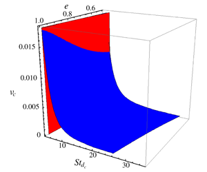
The master phase diagram in $(\unicode[STIX]{x1D708},e,St_{d})$ space, delineating the regions of existence of the (i) ignited and (ii) quenched states and (iii) their coexistence (I+Q). The ignited and quenched states exist to the right and left, respectively, of the ‘blue’ and ‘red’ surfaces; these critical surfaces are determined analytically using ordering analysis in §§ 3.1.1 and 3.1.2 respectively. The phase diagram for purely elastic collisions ($e=1$) is shown in panel (b), where the predictions from the works of Saha & Alam (Reference Saha and Alam2017) (dotted line), Tsao & Koch (Reference Tsao and Koch1995) (dashed line) and Sangani et al. (Reference Sangani, Mo, Tsao and Koch1996) (dot–dashed line) are also superimposed. The filled circles represent DSMC simulation results of Tsao & Koch (Reference Tsao and Koch1995); the solitary diamond symbol represents the present data for $\unicode[STIX]{x1D708}=5\times 10^{-4}$ as measured from figure 2(b). Panel (c) represents the projection of panel ($a$) at $e=0.5$. The ‘star’ symbols in panels (b,c) represent the ‘exact’ phase boundaries obtained from the numerical solution of (3.1).

For parameter values of figure 2(a) with $\unicode[STIX]{x1D708}=2\times 10^{-4}$ (i.e. in the bistable regime), figure 3 displays how the ignited or quenched states can be reached in simulations, depending on initial conditions. When the simulation is prepared to start with a high/low temperature ($T_{initial}>T_{is}$, or, $T_{initial}\sim T_{qs}$), the final equilibrium state corresponds to the ignited/quenched state, see the upper and lower solid lines, respectively, in figure 3 – this overall picture is similar to that shown in figure 1. However, an initial state with an intermediate temperature $T_{qs}\ll T_{initial}\ll T_{is}$ can evolve in time to result in accessing either the ignited (the dashed line in main panel) or the quenched (the dot-dash line in inset) state. In particular, the dashed line in figure 3 indicates that the temperature drops sharply at $\dot{\unicode[STIX]{x1D6FE}}t\sim 200$, implying that the system is trying to reach the Q-state; but the stochasticity inherent in DSMC simulations brings the temperature up quickly, which continues to increase with time, eventually reaching the I-state. On the other hand, with an initial temperature ‘almost’ identical to the initial state for the dashed line in figure 3, its inset indicates that the system eventually settles to the Q-state.

Focussing on the dilute regime of figure 2(a), the Stokes-number dependence of granular temperature is shown in figure 2(b) for a particle volume fraction of $\unicode[STIX]{x1D708}=5\times 10^{-4}$ with $e=1$; while the numerical solution of (3.1) is denoted by the solid line, the dashed line corresponds to the theory of Tsao & Koch (Reference Tsao and Koch1995). For a quantitative comparison, the DSMC simulation data are also superimposed as filled circles (Tsao & Koch Reference Tsao and Koch1995) and open diamonds (present simulation) in figure 2(b). Clearly, the present theory, with dense-gas corrections along with anisotropic Maxwellian distribution function, provides a better agreement for the quenched-state temperature $T_{qs}$ with the simulation data. In particular, the critical Stokes number ($St^{c_{2}}$) for the limit point of ‘quenched$\rightarrow$ignited’ transition, marked by an upward arrow in figure 2(b), is well predicted by the present theory – this is despite the fact that this transition occurs in a dilute ($\unicode[STIX]{x1D708}<0.02$, see panel $a$) suspension. The critical Stokes number ($St^{c_{1}}$) for the limit point of ‘ignited$\rightarrow$quenched’ transition, marked by a downward arrow in figure 2(b), is also well predicted by the present theory as well as by Tsao & Koch (Reference Tsao and Koch1995) and Saha & Alam (Reference Saha and Alam2017) for the parameter values mentioned. These two critical Stokes numbers ($St^{c_{1}}$ and $St^{c_{2}}$) are determined analytically in §§ 3.1.1 and 3.1.2, respectively.

3.1.1 Ignited-to-quenched transition: $St^{c_{1}}$

Referring to figure 2(b), the critical Stokes number $St_{d}=St_{d}^{c_{1}}$ for ‘ignited-to-quenched’ transition provides a lower bound for the existence of the ignited state, the quenched state is the only admissible solution at $St<St_{d}^{c_{1}}$ and, by definition, $\unicode[STIX]{x1D709}\gg 1$ along this limit point. With the latter assumption and considering only leading-order terms in (3.1), we arrive at the following quadratic equation

(3.2)$$\begin{eqnarray}\displaystyle \mathfrak{a}St_{d}^{4}+\mathfrak{b}St_{d}^{2}+\mathfrak{c}=0, & & \displaystyle\end{eqnarray}$$

to determine $St_{d}^{c_{1}}$; the coefficients of (3.2) are given in § B.1 (in the supplementary material). The solution of (3.2) is marked in figure 4(a) as a red surface in the three-dimensional $(St_{d},\unicode[STIX]{x1D708},e)$ space. This critical surface $T(St_{d}^{c_{1}},\unicode[STIX]{x1D708},e)$ represents the loci of the upper limit point of figure 2(b) where the unstable and ignited solution branches meet; to the left of this surface, the solution belongs to the quenched state.

3.1.2 Quenched-to-ignited transition: $St^{c_{2}}$

The critical Stokes number $St_{d}^{c_{2}}$ for ‘quenched-to-ignited’ transition (i.e. the lower limit point in figure 2b) represents an upper bound for the existence of the quenched state; the quenched and the unstable branches meet at this limit point on which we must have $\unicode[STIX]{x1D709}\sim O(1)$. Using this argument and applying an ordering analysis on each term of (3.1), we obtain

(3.3a)$$\begin{eqnarray}\displaystyle & \displaystyle {\mathcal{G}}(\unicode[STIX]{x1D709}_{c})\approx a_{4}\unicode[STIX]{x1D709}^{4}+a_{3}\unicode[STIX]{x1D709}^{3}+a_{2}\unicode[STIX]{x1D709}^{2}+a_{1}\unicode[STIX]{x1D709}=0=a_{4}\unicode[STIX]{x1D709}^{3}+a_{3}\unicode[STIX]{x1D709}^{2}+a_{2}\unicode[STIX]{x1D709}+a_{1}=0, & \displaystyle\end{eqnarray}$$

(3.3b)$$\begin{eqnarray}\displaystyle & \displaystyle {\displaystyle \frac{\text{d}{\mathcal{G}}}{\text{d}\unicode[STIX]{x1D709}}}(\unicode[STIX]{x1D709}_{c})\approx 3a_{4}\unicode[STIX]{x1D709}^{2}+2a_{3}\unicode[STIX]{x1D709}+a_{2}=0, & \displaystyle\end{eqnarray}$$

at leading order, where

(3.4)$$\begin{eqnarray}\left.\begin{array}{@{}c@{}}a_{4}=-6890625(13-9e)(1+e)(107+193e)\unicode[STIX]{x03C0}^{7/2}St_{d}^{5}\unicode[STIX]{x1D708}g_{0},\\ a_{3}=5788125000(13-9e)\unicode[STIX]{x03C0}^{4}St_{d}^{2},\\ a_{2}=-165375000(13-9e)(1+e)(1+3e)\unicode[STIX]{x03C0}^{7/2}St_{d}^{5}\unicode[STIX]{x1D708}g_{0},\\ a_{1}=-196000000(13-9e)(1+e)^{2}\unicode[STIX]{x03C0}^{3}St_{d}^{5}\unicode[STIX]{x1D708}g_{0}.\end{array}\right\}\end{eqnarray}$$

The solution of (3.3b) is

(3.5)$$\begin{eqnarray}\unicode[STIX]{x1D709}_{c}={\displaystyle \frac{2\left[140\sqrt{\unicode[STIX]{x03C0}}+\sqrt{2}\sqrt{9800\unicode[STIX]{x03C0}-(1+e)^{2}(1+3e)(107+193e)St_{d}^{6}\unicode[STIX]{x1D708}^{2}g_{0}^{2}}\right]}{(1+e)(107+193e)St^{3}\unicode[STIX]{x1D708}g_{0}}},\end{eqnarray}$$

which represents the critical temperature for the ‘quenched-to-ignited’ transition. Now, under the assumption $St_{d}^{3}\unicode[STIX]{x1D708}g_{0}\ll 1$ with $\sqrt{1-x}\approx 1-x/2$, (3.5) simplifies to

(3.6)

The over-braced term in (

3.6

) is the finite-density higher-order correction over our previous work (Saha & Alam Reference Saha and Alam2017), and removing this term along with the limit of $g_{0}(\unicode[STIX]{x1D708}\rightarrow 0)\rightarrow 1$ yields an expression for this critical temperature $\unicode[STIX]{x1D709}_{c}=560\sqrt{\unicode[STIX]{x03C0}}/(1+e)(107+193e)St^{3}\unicode[STIX]{x1D708}$, which is identical to the dilute-limit solution of Saha & Alam (Reference Saha and Alam2017).

On substituting (3.6) into (3.3a), we obtain

(3.7)$$\begin{eqnarray}\displaystyle & & \displaystyle 2(1+e)^{4}(107+193e)^{2}(St_{d}^{3}\unicode[STIX]{x1D708}g_{0})^{3}+\overbrace{945\unicode[STIX]{x03C0}(1+e)^{2}(1+3e)(107+193e)(St_{d}^{3}\unicode[STIX]{x1D708}g_{0})^{2}}^{}\nonumber\\ \displaystyle & & \displaystyle \quad -\,6174000\unicode[STIX]{x03C0}^{2}=0.\end{eqnarray}$$

The solution of (3.7) is plotted as a blue surface in figure 4(a) and it provides a measure of the upper bound for the quenched state to exist in the ($St_{d},\unicode[STIX]{x1D708},e$)-space. Above this critical surface, the ignited state is the only feasible solution and both the states can co-exist below this surface.

In figure 4(a), the blue surface determining $St_{d}^{c_{2}}(\unicode[STIX]{x1D708},e)$ meets the red surface determining $St_{d}^{c_{1}}(\unicode[STIX]{x1D708},e)$ at some density yielding a critical curve which marks the point of transition between multiple and unique solutions. It is clear that this limiting curve is a sharply decreasing function of inelasticity (i.e. increasing function of $e$). The loci of two limit points in the ($St_{d},\unicode[STIX]{x1D708}$)-plane can be identified in figures 4(b) and 4(c), respectively, for $e=1$ and $e=0.5$. The predictions from the works of Tsao & Koch (Reference Tsao and Koch1995) (dashed line), Sangani et al. (Reference Sangani, Mo, Tsao and Koch1996) (dot-dashed line) and Saha & Alam (Reference Saha and Alam2017) (dotted line) are also superimposed in panel ($b$) for a quantitative comparison with the present theory. Note that the DSMC data of Tsao & Koch (Reference Tsao and Koch1995) are marked as filled circles and those of the present simulation are marked by the diamond symbol (as obtained from figure 2$b$). Figure 4(b) confirms that the present theory predicts $St_{d}^{3}\unicode[STIX]{x1D708}\approx 2.07$ (for $e=1$) which is closest to the simulation result (Tsao & Koch Reference Tsao and Koch1995). On the other hand, all previous works (including Saha & Alam (Reference Saha and Alam2017)) are unable to provide a quantitative agreement for $St^{c_{2}}$. For example, the inclusion of dense-gas effects in the Grad-moment theory of Sangani et al. (Reference Sangani, Mo, Tsao and Koch1996) grossly over-predicts the simulation data for $St^{c_{2}}$ as seen from the right-most dot-dashed line in figure 4(b) – in fact, Sangani et al.’s (Reference Sangani, Mo, Tsao and Koch1996) theory deviates more from the related dilute theory of Tsao & Koch (Reference Tsao and Koch1995). To conclude, the present theory significantly improves the bound on $St^{c_{2}}$ and yields the closest agreement with simulation as confirmed by the solid lines in figure 4(b,c).

Table 1.

Summary of predictions for $St^{c_{2}}(e=1)$ from different theories; see figure 4(b,c) for line types representing different theories.

The differences between the present theory and our previous work on dilute suspensions (Saha & Alam Reference Saha and Alam2017) can be understood by considering the over-braced term in (3.7) that represents the finite-density effects appearing beyond the leading order. With the assumption $St_{d}^{3}\unicode[STIX]{x1D708}g_{0}\ll 1$, the second term of (3.7) dominates over the first term, yielding an equation for the critical surface as

(3.8)$$\begin{eqnarray}(St_{d}^{c_{2}})^{3}\unicode[STIX]{x1D708}_{c}g_{0}=\left({\displaystyle \frac{1234800\unicode[STIX]{x03C0}}{189(1+e)^{2}(1+3e)(107+193e)}}\right)^{1/2}.\end{eqnarray}$$

On the other hand, removing the over-braced term from (3.7), we get

(3.9)$$\begin{eqnarray}(St^{c_{2}})^{3}\unicode[STIX]{x1D708}_{c}g_{0}=\left({\displaystyle \frac{3087000\unicode[STIX]{x03C0}^{2}}{(1+e)^{4}(107+193e)^{2}}}\right)^{1/3},\end{eqnarray}$$

which coincides with the expression for $St^{c_{2}}$ of Saha & Alam (Reference Saha and Alam2017) for a dilute suspension. Therefore, the inclusion of finite-density effects makes (3.7) singular, resulting in different expressions (3.8) and (3.9) for the ‘quenched-to-ignited’ transition surface. The underlying quantitative differences can be ascertained from table 1, which summarizes different theoretical predictions for $St^{c_{2}}$ at $e=1$. Note that the numerical solution of (3.7) provides a more accurate prediction for $St^{c_{2}}$ than the analytical solution (3.8), as confirmed from a comparison with the simulation data in figure 4(b,c).

Figure 5.

Co-existence of ignited (high temperature) and quenched (low temperature) states in particle simulations of gas–solid suspensions: time evolution of the granular temperature ($\sqrt{T}$) for effective Stokes numbers of $St_{d}=9$ and $10$; the particle volume fraction is $\unicode[STIX]{x1D708}=5\times 10^{-4}$ and the restitution coefficient is $e=1$. Two plateaus of low and high temperatures refer to ‘quenched’ and ‘ignited’ states, respectively.

3.2 Solution for the second-moment anisotropy ($\unicode[STIX]{x1D702},\unicode[STIX]{x1D719},\unicode[STIX]{x1D706}^{2}$)

The solution for the non-coaxiality angle can be obtained by subtracting (2.27b) from (2.27a) and is given by,

(3.10)$$\begin{eqnarray}\displaystyle \cot 2\unicode[STIX]{x1D719}={\displaystyle \frac{12(3-e)(1+e)\unicode[STIX]{x1D708}g_{0}\sqrt{T}}{5\sqrt{\unicode[STIX]{x03C0}}}}+{\displaystyle \frac{2}{St_{d}}}. & & \displaystyle\end{eqnarray}$$

Once the granular temperature $(T)$ and the non-coaxiality angle $(\unicode[STIX]{x1D719})$ are determined from (3.1) and (3.10), respectively, the remaining equations of (2.27) can be manipulated to yield closed-form solutions for two other anisotropy parameters $(\unicode[STIX]{x1D702},\unicode[STIX]{x1D706}^{2})$. Note that the effect of the gas phase on $\unicode[STIX]{x1D719}$ occurs explicitly via the second term in (3.10); however, the quenched-state terms ($\aleph _{\unicode[STIX]{x1D6FC}\unicode[STIX]{x1D6FD}}^{qs}$) do not appear in (3.10), but their effects occur implicitly via $T$ in (3.1).

The temperature anisotropy $\unicode[STIX]{x1D702}$ satisfies a quadratic equation $b_{2}\unicode[STIX]{x1D702}^{2}+b_{1}\unicode[STIX]{x1D702}+b_{0}=0$, where

(3.11a)$$\begin{eqnarray}\displaystyle & \hspace{-24.0pt}\displaystyle b_{2}={\displaystyle \frac{3(1-e^{2})}{5\sqrt{\unicode[STIX]{x03C0}}}}\unicode[STIX]{x1D708}g_{0}T^{3/2}, & \displaystyle\end{eqnarray}$$

(3.11b)$$\begin{eqnarray}\displaystyle & \hspace{-24.0pt}\displaystyle b_{1}=-\left(1-{\textstyle \frac{2}{5}}(1+e)(1-3e)\unicode[STIX]{x1D708}g_{0}\right)T\cos 2\unicode[STIX]{x1D719}, & \displaystyle\end{eqnarray}$$

(3.11c)$$\begin{eqnarray}\displaystyle & \hspace{-24.0pt}\displaystyle b_{0}={\displaystyle \frac{3T}{St_{d}}}+{\displaystyle \frac{6(1-e^{2})}{\sqrt{\unicode[STIX]{x03C0}}}}\unicode[STIX]{x1D708}g_{0}T^{3/2}-{\displaystyle \frac{16}{35\unicode[STIX]{x03C0}}}(1+e)^{2}\unicode[STIX]{x1D708}g_{0}-{\displaystyle \frac{2(1+e)(1+3e)}{5\sqrt{\unicode[STIX]{x03C0}}}}\unicode[STIX]{x1D708}g_{0}\sqrt{T}. & \displaystyle\end{eqnarray}$$

$\unicode[STIX]{x1D702}$

(3.12a)$$\begin{eqnarray}\displaystyle \unicode[STIX]{x1D702} & \stackrel{e\neq 1}{=} & \displaystyle -{\displaystyle \frac{b_{1}}{2b_{2}}}-{\displaystyle \frac{1}{b_{2}}}\sqrt{b_{1}^{2}-4b_{0}b_{2}},\end{eqnarray}$$

(3.12b)$$\begin{eqnarray}\displaystyle & \stackrel{e=1}{=} & \displaystyle -{\displaystyle \frac{b_{0}}{b_{1}}},\end{eqnarray}$$

$e=1$

$St_{d}<\infty$

$T$

$St_{d}\rightarrow \infty$

$e=1$

$\unicode[STIX]{x1D706}^{2}$

(3.13)$$\begin{eqnarray}\unicode[STIX]{x1D706}^{2}={\displaystyle \frac{\unicode[STIX]{x1D702}}{\sin 2\unicode[STIX]{x1D719}}}-{\displaystyle \frac{4}{35}}(1+e)^{2}\unicode[STIX]{x1D708}g_{0}T^{-1}-\left(1-{\displaystyle \frac{2}{5}}(1+e)(1-3e)\unicode[STIX]{x1D708}g_{0}\right),\end{eqnarray}$$

and the dimensionless excess temperature is

(3.14)$$\begin{eqnarray}{\displaystyle \frac{T^{ex}}{T}}\stackrel{def}{=}{\displaystyle \frac{T-T_{z}}{T}}=2\unicode[STIX]{x1D706}^{2}.\end{eqnarray}$$

Based on the solutions given in (3.10)–(3.14), the density dependences of $\unicode[STIX]{x1D702}$, $\unicode[STIX]{x1D719}$ and $\unicode[STIX]{x1D706}^{2}$ are displayed in figures 6(a), 6(b) and 6(c), respectively; the Stokes number is set to $St=7$ and the restitution coefficient is $e=0.9$, as in figure 2(a). Excellent agreement with the simulation data is found for all three anisotropy parameters on both the ignited and quenched branches over the whole range of density ($\unicode[STIX]{x1D708}\leqslant 0.5$). Note that the quenched-state solution is highly anisotropic compared to its ignited-state counterpart since

(3.15)$$\begin{eqnarray}(\unicode[STIX]{x1D702},\unicode[STIX]{x1D719},\unicode[STIX]{x1D706}^{2})_{quenched}>(\unicode[STIX]{x1D702},\unicode[STIX]{x1D719},\unicode[STIX]{x1D706}^{2})_{ignited},\end{eqnarray}$$

as confirmed in figure 6. On the ignited branch, however, the variations of $(\unicode[STIX]{x1D702},\unicode[STIX]{x1D719},\unicode[STIX]{x1D706}^{2})$ with density are found to be non-monotonic, with the respective maxima occurring at the limit point of ‘ignited-to-quenched’ transition. Recall that the shear-induced collisions are responsible for the origin of the second moment in the quenched state in which the particles largely follow the fluid motion. Such shear-driven particle collisions can occur only along preferred directions, resulting in a highly anisotropic second-moment tensor compared to its ignited counterpart, see (3.15).

Figure 6.

Same as figure 2(a), but for the variations of the second-moment anisotropy parameters: (a) the shear-plane temperature anisotropy $\unicode[STIX]{x1D702}$, (b) the non-coaxiality angle $\unicode[STIX]{x1D719}$ (in degrees) and (c) the excess temperature along the vorticity direction $\unicode[STIX]{x1D706}^{2}$. Parameter values are $St=7$ and $e=0.9$.

Figure 7.

Variations of (a,d) shear-plane temperature anisotropy $\unicode[STIX]{x1D702}$, (b,e) the non-coaxiality angle $\unicode[STIX]{x1D719}$ and (c,f) the excess temperature $T_{z}^{ex}/T=2\unicode[STIX]{x1D706}^{2}$ with Stokes number $St_{d}$. Parameter values are $\unicode[STIX]{x1D708}=5\times 10^{-4}$ and (a–c) $e=1$ and (d–f) $e=0.9$ (dotted line) and $0.5$ (dashed line, and the diamonds denote the present simulation data).

Focussing on the co-existence regime of figure 6, we show the $St$-dependence of $(\unicode[STIX]{x1D702},\unicode[STIX]{x1D719},\unicode[STIX]{x1D706}^{2})$ in figure 7 for a particle volume fraction of $\unicode[STIX]{x1D708}=5\times 10^{-4}$ (as in figure 2b), with the restitution coefficient being set to $e=1$ in (a–c) and $e=(0.5,0.9)$ in (d–f). It is seen that while the second-moment anisotropy increases with increasing $St_{d}$ on the quenched branch, it decreases sharply on the ignited branch; overall there is excellent agreement of theoretical predictions (3.10)–(3.14) with the present simulation data over a range of $St_{d}$ for both elastic (a–c) and inelastic particles (d–f). Comparing the dashed and dotted lines in figure 7(d–f) for $e=0.5$ and $0.9$, respectively, we find that the inelasticity markedly increases the values of $(\unicode[STIX]{x1D702},\unicode[STIX]{x1D719},\unicode[STIX]{x1D706}^{2})$ on the ignited branch. Note that the anisotropy of the quenched solution is hardly affected by inelasticity, which is expected since the origin of the quenched solution is tied to shear-induced collisions.

3.3 Burnett-order stress tensor and the transport coefficients

Since we have retained terms up to second order in the shear rate and three anisotropy parameters in the second-moment balance (2.27), the stress tensor and the related transport coefficients should be evaluated at the Burnett order. Retaining terms up to the second order $O(\unicode[STIX]{x1D702}^{i}\unicode[STIX]{x1D706}^{j}R^{k}\sin ^{l}2\unicode[STIX]{x1D719},\;i+j+k+l\leqslant 2)$, the diagonal elements of the dimensionless stress tensor,

(3.16)$$\begin{eqnarray}\unicode[STIX]{x1D64B}^{\ast }={\displaystyle \frac{\tilde{\unicode[STIX]{x1D64B}}}{\unicode[STIX]{x1D70C}_{p}\unicode[STIX]{x1D708}(\dot{\unicode[STIX]{x1D6FE}}\unicode[STIX]{x1D70E}/2)^{2}}},\end{eqnarray}$$

have the following form

(3.17a)$$\begin{eqnarray}\displaystyle \hspace{-24.0pt}P_{xx}^{\ast } & = & \displaystyle T\left[(1+\unicode[STIX]{x1D706}^{2}+\unicode[STIX]{x1D702}\sin 2\unicode[STIX]{x1D719})\right.\nonumber\\ \displaystyle \hspace{-24.0pt} & & \displaystyle \left.+\,{\displaystyle \frac{2(1+e)\unicode[STIX]{x1D708}g_{0}}{35}}\left\{35+14\unicode[STIX]{x1D706}^{2}+14\unicode[STIX]{x1D702}\sin 2\unicode[STIX]{x1D719}+96R^{2}+{\displaystyle \frac{48}{\sqrt{\unicode[STIX]{x03C0}}}}\unicode[STIX]{x1D702}R\cos 2\unicode[STIX]{x1D719}\right\}\right],\end{eqnarray}$$

(3.17b)$$\begin{eqnarray}\displaystyle \hspace{-24.0pt}P_{yy}^{\ast } & = & \displaystyle T\left[(1+\unicode[STIX]{x1D706}^{2}-\unicode[STIX]{x1D702}\sin 2\unicode[STIX]{x1D719})\right.\nonumber\\ \displaystyle \hspace{-24.0pt} & & \displaystyle +\,\left.{\displaystyle \frac{2(1+e)\unicode[STIX]{x1D708}g_{0}}{35}}\left\{35+14\unicode[STIX]{x1D706}^{2}-14\unicode[STIX]{x1D702}\sin 2\unicode[STIX]{x1D719}+96R^{2}+{\displaystyle \frac{48}{\sqrt{\unicode[STIX]{x03C0}}}}\unicode[STIX]{x1D702}R\cos 2\unicode[STIX]{x1D719}\right\}\right],\end{eqnarray}$$

(3.17c)$$\begin{eqnarray}\displaystyle \hspace{-24.0pt}P_{zz}^{\ast } & = & \displaystyle T\left[(1-2\unicode[STIX]{x1D706}^{2})+{\displaystyle \frac{2(1+e)\unicode[STIX]{x1D708}g_{0}}{35}}\left\{35-28\unicode[STIX]{x1D706}^{2}+32R^{2}+{\displaystyle \frac{16}{\sqrt{\unicode[STIX]{x03C0}}}}\unicode[STIX]{x1D702}R\cos 2\unicode[STIX]{x1D719}\right\}\right],\end{eqnarray}$$

$\unicode[STIX]{x1D648}$

(3.18a-d)$$\begin{eqnarray}\unicode[STIX]{x1D702}\equiv \unicode[STIX]{x1D702}(\unicode[STIX]{x1D708},e,St),\quad \unicode[STIX]{x1D719}\equiv \unicode[STIX]{x1D719}(\unicode[STIX]{x1D708},e,St),\quad \unicode[STIX]{x1D706}\equiv \unicode[STIX]{x1D706}(\unicode[STIX]{x1D708},e,St),\quad R\equiv R(\unicode[STIX]{x1D708},e,St)\end{eqnarray}$$

that have been evaluated in §§ 3.1 and 3.2. Recall that $R=\dot{\unicode[STIX]{x1D6FE}}\unicode[STIX]{x1D70E}/8\sqrt{\tilde{T}}\equiv 1/4\sqrt{T}$ is the dimensionless shear rate and $T=\tilde{T}/(\dot{\unicode[STIX]{x1D6FE}}\unicode[STIX]{x1D70E}/2)^{2}\equiv T(\unicode[STIX]{x1D708},e,St)$ is the dimensionless temperature. The related fourth-order, $O(\unicode[STIX]{x1D702}^{i}\unicode[STIX]{x1D706}^{j}R^{k}\sin ^{l}2\unicode[STIX]{x1D719},\;i+j+k+l\leqslant 4)$, expressions for $P_{\unicode[STIX]{x1D6FC}\unicode[STIX]{x1D6FD}}$ are given in (A 22)–(A 24) of § A.1 (in the supplementary material) that will be used in § 4.

By summing (3.17a)–(3.17c), the expression for the particle-phase pressure (in dimensionless form) is found as

(3.19)$$\begin{eqnarray}p={\displaystyle \frac{1}{3}}P_{\unicode[STIX]{x1D6FC}\unicode[STIX]{x1D6FC}}=T\left[1+2(1+e)\unicode[STIX]{x1D708}g_{0}+\underbrace{{\displaystyle \frac{64(1+e)\unicode[STIX]{x1D708}g_{0}}{15}}\left(1+{\displaystyle \frac{1}{2\sqrt{\unicode[STIX]{x03C0}}}}{\displaystyle \frac{\unicode[STIX]{x1D702}}{R}}\cos 2\unicode[STIX]{x1D719}\right)R^{2}}_{}\right].\end{eqnarray}$$

The first two terms represent the Navier–Stokes-order pressure of a dense gas,

(3.20)$$\begin{eqnarray}p_{NS}=T[1+2(1+e)\unicode[STIX]{x1D708}g_{0}],\end{eqnarray}$$

while the under-braced terms in (3.19) are second order in the shear rate, $O(R^{2})$, representing its Burnett-order contribution

(3.21)$$\begin{eqnarray}p_{(II)}={\displaystyle \frac{4(1+e)\unicode[STIX]{x1D708}g_{0}}{15}}\left(1+{\displaystyle \frac{1}{2\sqrt{\unicode[STIX]{x03C0}}}}{\displaystyle \frac{\unicode[STIX]{x1D702}}{R}}\cos 2\unicode[STIX]{x1D719}\right),\end{eqnarray}$$

such that $p=p_{NS}+p_{(II)}+\cdots \,.$ It must be noted that the effect of the gas phase on $p_{NS}$ remains implicit via the Stokes dependence of granular temperature $T=T(\unicode[STIX]{x1D708},e,St)$. Note further that the functional form of the kinetic pressure ($\tilde{p}^{k}=\tilde{\unicode[STIX]{x1D70C}}\tilde{T}$) remains the same at all orders, the Burnett-order contributions appear explicitly in the collisional component ($p^{c}$) of pressure.

3.3.1 Shear stress and the particle-phase shear viscosity

Retaining terms up to the third order $O(\unicode[STIX]{x1D702}^{i}\unicode[STIX]{x1D706}^{j}R^{k}\sin ^{l}2\unicode[STIX]{x1D719},\;i+j+k+l\leqslant 3)$, the dimensionless shear stress can be written as

(3.22)$$\begin{eqnarray}\displaystyle P_{xy}^{\ast }={\displaystyle \frac{\tilde{P}_{xy}}{\unicode[STIX]{x1D70C}_{p}\unicode[STIX]{x1D708}\dot{\unicode[STIX]{x1D6FE}}^{2}(\unicode[STIX]{x1D70E}/2)^{2}}} & = & \displaystyle -\unicode[STIX]{x1D702}\cos 2\unicode[STIX]{x1D719}T-{\displaystyle \frac{4(1+e)\unicode[STIX]{x1D708}g_{0}T}{5\sqrt{\unicode[STIX]{x03C0}}}}\Bigg[R\left\{8+\sqrt{\unicode[STIX]{x03C0}}{\displaystyle \frac{\unicode[STIX]{x1D702}\cos 2\unicode[STIX]{x1D719}}{R}}\right\}\nonumber\\ \displaystyle & & \displaystyle +\,\underbrace{{\displaystyle \frac{4}{21}}R^{3}\left\{32-{\displaystyle \frac{\unicode[STIX]{x1D702}^{2}}{R^{2}}}(2+\cos 4\unicode[STIX]{x1D719})+12{\displaystyle \frac{\unicode[STIX]{x1D706}^{2}}{R^{2}}}\right\}}_{}\Bigg],\end{eqnarray}$$

where the under-braced terms belong to the third (super-Burnett) order that must be included to evaluate the shear viscosity at the Burnett order. Note that the even-order terms do not contribute to shear stress, and since (3.22) contains terms up to the super-Burnett order, the neglected terms in (3.22) belong to fifth order and beyond.

The dimensionless shear viscosity of the particle phase, up to Burnett order, can be obtained from (3.22),

(3.23)$$\begin{eqnarray}\displaystyle \unicode[STIX]{x1D707} & \stackrel{def}{=} & \displaystyle -{\displaystyle \frac{\tilde{P}_{xy}/\dot{\unicode[STIX]{x1D6FE}}}{\unicode[STIX]{x1D70C}_{p}\unicode[STIX]{x1D708}\dot{\unicode[STIX]{x1D6FE}}(\unicode[STIX]{x1D70E}/2)^{2}}}\equiv -P_{xy}^{\ast }\nonumber\\ \displaystyle & = & \displaystyle \left({\displaystyle \frac{\unicode[STIX]{x1D702}}{4R}}\cos 2\unicode[STIX]{x1D719}\right)\sqrt{T}+{\displaystyle \frac{4(1+e)\unicode[STIX]{x1D708}g_{0}\sqrt{T}}{5\sqrt{\unicode[STIX]{x03C0}}}}\left[\left(2+{\displaystyle \frac{\sqrt{\unicode[STIX]{x03C0}}}{4}}\left({\displaystyle \frac{\unicode[STIX]{x1D702}}{R}}\cos 2\unicode[STIX]{x1D719}\right)\right)\right.\nonumber\\ \displaystyle & & \displaystyle \left.\quad +{\displaystyle \frac{R^{2}}{21}}\left\{32-{\displaystyle \frac{\unicode[STIX]{x1D702}^{2}}{R^{2}}}\left(2+\cos 4\unicode[STIX]{x1D719}\right)+12{\displaystyle \frac{\unicode[STIX]{x1D706}^{2}}{R^{2}}}\right\}\right].\end{eqnarray}$$

While the first term in (3.23) represents the kinetic part of viscosity, the remaining $g_{0}$-dependent terms represent the collisional viscosity. This (3.23) is the Burnett-order expression for the particle-phase shear viscosity of a moderately dense gas–solid suspension valid up to second order in the shear rate; the NS-order viscosity follows by removing the $O(R^{2})$ term from (3.23). Note that the effects of the gas phase and the shear-driven collisions are implicit in (3.23) via the $St$-dependence of the anisotropy parameters ($\unicode[STIX]{x1D702},\unicode[STIX]{x1D719},\unicode[STIX]{x1D706}^{2}$), as clarified in (3.18) and figures 6–7.

3.3.2 Normal-stress differences and their origin

On subtracting (3.17b) from (3.17a), we obtain the expression for the (dimensionless) first normal-stress difference as

(3.24)$$\begin{eqnarray}\displaystyle N_{1}=P_{xx}-P_{yy}=2\unicode[STIX]{x1D702}\sin 2\unicode[STIX]{x1D719}\left\{1+{\textstyle \frac{4}{5}}(1+e)\unicode[STIX]{x1D708}g_{0}\right\}T. & & \displaystyle\end{eqnarray}$$

Note that $N_{1}\rightarrow 0$ in the limit of vanishing anisotropy, $(\unicode[STIX]{x1D702},\unicode[STIX]{x1D719})\rightarrow 0$, of the second-moment tensor on the shear plane. Therefore the origin of the first normal-stress difference is tied to the shear-plane anisotropy of $\unicode[STIX]{x1D648}$. According to the present theory, $N_{1}$ is positive and maximal in a dilute suspension ($\unicode[STIX]{x1D708}\rightarrow 0$), but vanishes in the dense limit ($\unicode[STIX]{x1D708}\rightarrow \unicode[STIX]{x1D708}_{max}$) since $(\unicode[STIX]{x1D702},\unicode[STIX]{x1D719})\rightarrow 0$ in the latter limit. These overall findings mimic those in a ‘dry’ granular ($St\rightarrow \infty$) suspension (Saha & Alam Reference Saha and Alam2016).

The expression for the (dimensionless) second normal-stress difference is given by

(3.25)$$\begin{eqnarray}\displaystyle N_{2} & = & \displaystyle P_{yy}-P_{zz}=\left(3\unicode[STIX]{x1D706}^{2}-\unicode[STIX]{x1D702}\sin 2\unicode[STIX]{x1D719}\right)T\nonumber\\ \displaystyle & & \displaystyle +\,{\displaystyle \frac{4(1+e)\unicode[STIX]{x1D708}g_{0}}{35}}\left[32\left(1+{\displaystyle \frac{1}{2\sqrt{\unicode[STIX]{x03C0}}}}{\displaystyle \frac{\unicode[STIX]{x1D702}}{R}}\cos 2\unicode[STIX]{x1D719}\right)R^{2}+21\unicode[STIX]{x1D706}^{2}-7\unicode[STIX]{x1D702}\sin 2\unicode[STIX]{x1D719}\right]T,\end{eqnarray}$$

with the first and second terms representing its kinetic and collisional components, respectively. It is clear that the kinetic part of $N_{2}$, which dominates in the dilute limit, is zero when $(\unicode[STIX]{x1D702},\unicode[STIX]{x1D719},\unicode[STIX]{x1D706}^{2})\rightarrow 0$ that corresponds to an isotropic second-moment tensor, or, when $3\unicode[STIX]{x1D706}^{2}=\unicode[STIX]{x1D702}\sin 2\unicode[STIX]{x1D719}$. On the other hand, even if the second-moment tensor is isotropic, i.e. $(\unicode[STIX]{x1D702},\unicode[STIX]{x1D719},\unicode[STIX]{x1D706}^{2})\rightarrow 0$, (3.25) yields

(3.26)$$\begin{eqnarray}\displaystyle N_{2}={\displaystyle \frac{8(1+e)\unicode[STIX]{x1D708}g_{0}}{35}}\left(1+{\displaystyle \frac{1}{2\sqrt{\unicode[STIX]{x03C0}}}}{\displaystyle \frac{\unicode[STIX]{x1D702}}{R}}\cos 2\unicode[STIX]{x1D719}\right)\geqslant 0. & & \displaystyle\end{eqnarray}$$

A closer look at (3.17b)–(3.17c) reveals that the Burnett-order collisional anisotropy is responsible for finite (and positive) values of $N_{2}$ in a dense granular suspension.

3.3.3 Collisional dissipation at Burnett order

Under homogeneous shearing, the non-zero elements of the source of the second-moment tensor (2.13) have the following expressions:

(3.27a)$$\begin{eqnarray}\displaystyle \aleph _{xx} & = & \displaystyle A_{xx}+\widehat{E}_{xx}+\widehat{G}_{xx}+\dot{\unicode[STIX]{x1D6FE}}\unicode[STIX]{x1D6E9}_{xy},\end{eqnarray}$$

(3.27b)$$\begin{eqnarray}\displaystyle \aleph _{yy} & = & \displaystyle A_{yy}+\widehat{E}_{yy}+\widehat{G}_{yy}-\dot{\unicode[STIX]{x1D6FE}}\unicode[STIX]{x1D6E9}_{xy},\end{eqnarray}$$

(3.27c)$$\begin{eqnarray}\displaystyle \aleph _{zz} & = & \displaystyle A_{zz}+\widehat{E}_{zz}+\widehat{G}_{zz},\end{eqnarray}$$

(3.27d)$$\begin{eqnarray}\displaystyle \aleph _{xy} & = & \displaystyle A_{xy}+\widehat{E}_{xy}+\widehat{G}_{xy}+{\displaystyle \frac{\dot{\unicode[STIX]{x1D6FE}}}{2}}\left(\unicode[STIX]{x1D6E9}_{yy}-\unicode[STIX]{x1D6E9}_{xx}\right).\end{eqnarray}$$

The algebraic expressions for these quantities, as functions of $(\unicode[STIX]{x1D708},e,T;\unicode[STIX]{x1D702},\unicode[STIX]{x1D719},\unicode[STIX]{x1D706}^{2})$ up to the Burnett order, are provided in appendix A (in the supplementary material).

The rate of collisional dissipation per unit volume is given by

(3.28a)$$\begin{eqnarray}{\mathcal{D}}=-{\displaystyle \frac{1}{2}}\aleph _{\unicode[STIX]{x1D6FC}\unicode[STIX]{x1D6FC}}=-{\displaystyle \frac{1}{2}}A_{\unicode[STIX]{x1D6FC}\unicode[STIX]{x1D6FC}}={\displaystyle \frac{3(1-e^{2})\unicode[STIX]{x1D70C}\unicode[STIX]{x1D708}g_{0}T^{3/2}}{\unicode[STIX]{x1D70E}\unicode[STIX]{x03C0}^{3/2}}}\left({\mathcal{H}}_{003}^{30}+{\mathcal{H}}_{003}^{12}\right)\equiv {\mathcal{D}}_{NS}+{\mathcal{D}}_{(II)},\end{eqnarray}$$

where

(3.29)$$\begin{eqnarray}{\mathcal{D}}_{NS}={\displaystyle \frac{12(1-e^{2})\unicode[STIX]{x1D70C}\unicode[STIX]{x1D708}g_{0}T^{3/2}}{\sqrt{\unicode[STIX]{x03C0}}\unicode[STIX]{x1D70E}}}\end{eqnarray}$$

is its Navier–Stokes-order expression, which coincides with the well-known expression in the literature (Jenkins & Richman Reference Jenkins and Richman1985), and its second-order contribution is

(3.30)$$\begin{eqnarray}{\mathcal{D}}_{(II)}={\displaystyle \frac{6(1-e^{2})\unicode[STIX]{x1D70C}\unicode[STIX]{x1D708}g_{0}T^{3/2}}{5\sqrt{\unicode[STIX]{x03C0}}\unicode[STIX]{x1D70E}}}\left[\unicode[STIX]{x1D702}^{2}+8R^{2}\left\{4+\sqrt{\unicode[STIX]{x03C0}}\left({\displaystyle \frac{\unicode[STIX]{x1D702}}{R}}\cos 2\unicode[STIX]{x1D719}\right)\right\}\right].\end{eqnarray}$$

It is interesting to note in (3.30) that the Burnett-order contribution to inelastic dissipation depends on the the shear-plane anisotropies ($\unicode[STIX]{x1D702},\unicode[STIX]{x1D719}$) but not on the excess temperature ($\unicode[STIX]{x1D706}^{2}$); the effect of $\unicode[STIX]{x1D706}^{2}$ on ${\mathcal{D}}$ appears at the quartic order in the shear rate (i.e. super–super–Burnett order).

Figure 8.

Variations of the particle-phase (a) shear viscosity $\unicode[STIX]{x1D707}$, (b) pressure $p$ and the scaled $(c)$ first (${\mathcal{N}}_{1}=N_{1}/p$) and (d) second (${\mathcal{N}}_{2}=N_{2}/p$) normal-stress differences with particle volume fraction ($\unicode[STIX]{x1D708}$) for $e=0.9$ and Stokes number $St=7$. The solid lines are present theoretical predictions (§ 3.3) and the symbols denote present simulation data.

3.4 Comparison of Burnett-order transport coefficients with simulation and their scalings with Stokes number

Figure 8 displays the density variations of (a) the shear viscosity ($\unicode[STIX]{x1D707}$, (3.23)), (b) the pressure ($p$, (3.19)) and (c,d) the ‘scaled’ first and second normal-stress differences, (${\mathcal{N}}_{1}=N_{1}/p$, (3.24) and ${\mathcal{N}}_{2}=N_{2}/p$, (3.25), both scaled by mean pressure) for a Stokes number of $St=7$ and a restitution coefficient of $e=0.9$. In each panel, the solid lines represent the theoretical predictions from the combined ‘ignited–quenched’ theory of § 3.3 and the symbols denote the present simulation data obtained using the DSMC method (Alam et al. Reference Alam, Saha and Gupta2019). For each field in figure 8, three different solution branches are found below a critical density of $\unicode[STIX]{x1D708}_{c}\approx 0.015$ for these parameter values – the magenta and blue lines correspond to the stable ‘quenched’ and ‘ignited’ states, respectively, whereas the red line correspond to the intermediate unstable branch. Overall, there is an excellent agreement between theory and simulation for all rheological fields in figure 8 including the density range over which the hysteresis is found. Figures 8(a) and 8(b) clarify that the density dependences of both viscosity (panel $a$) and pressure (panel $b$) mirror that of the granular temperature discussed in figure 2(a); this is expected since $\unicode[STIX]{x1D707}\propto \sqrt{T}$ and $p\propto T$. Therefore, in the co-existing regime, the states of ‘quenched’, ‘unstable’ and ‘ignited’, correspond to very small, intermediate and large values, respectively, of granular temperature, viscosity and pressure. On the other hand, figures 8(c) and 8(d) indicate that both normal-stress differences are large and small on the quenched and ignited branches, respectively – this implies that the quenched solutions are highly anisotropic (compared to their ignited counterparts) as characterized in figure 6 in terms of their second-moment anisotropy parameters ($\unicode[STIX]{x1D702},\unicode[STIX]{x1D719},\unicode[STIX]{x1D706}^{2}$).

On the quenched branch in figure 8(c,d), both ${\mathcal{N}}_{1}$ and ${\mathcal{N}}_{2}$ are maximal in the dilute limit and decrease slowly with increasing $\unicode[STIX]{x1D708}$ before the limit point is reached, beyond which only ignited solution exists. The first normal-stress difference on the ignited state varies non-monotonically with density, see figure 8(c) – ${\mathcal{N}}_{1}^{is}$ is maximal at the limit point density ($\unicode[STIX]{x1D708}=\unicode[STIX]{x1D708}_{c}$) and decreases with increasing and decreasing density about $\unicode[STIX]{x1D708}_{c}$. On the other hand, the ignited state ${\mathcal{N}}_{2}$ in figure 8(d) shows some interesting behaviour – ${\mathcal{N}}_{2}^{is}$ is negative in the dilute limit and is a slowing decreasing function of $\unicode[STIX]{x1D708}$, but changes its behaviour at the limit point $\unicode[STIX]{x1D708}=\unicode[STIX]{x1D708}_{c}$ and becomes an increasing function of $\unicode[STIX]{x1D708}$ beyond $\unicode[STIX]{x1D708}>\unicode[STIX]{x1D708}_{c}$ and thereafter undergoes a sign change at some finite density and increases up to a density of $\unicode[STIX]{x1D708}\sim 0.3$ and then decreases again but remains positive in the dense limit. The related simulation data in figure 8(d) confirm this complex dependence of ${\mathcal{N}}_{2}^{is}$ on density – note that the agreement between simulation and theory is qualitative for ${\mathcal{N}}_{2}^{is}$.

Figure 9.

Variations of (a,d) shear viscosity ($\unicode[STIX]{x1D707}$) (3.23), and the (b,e) first (${\mathcal{N}}_{1}=N_{1}/p$) (3.24) and (c,f) second (${\mathcal{N}}_{2}=N_{2}/p$) (3.25) normal-stress differences. The solid lines represent theoretical predictions and the symbols represent DSMC data; the quenched and ignited branches are marked by $Q$ and $I$, respectively. The particle volume fraction is $\unicode[STIX]{x1D708}=5\times 10^{-4}$ and the restitution coefficients are (a–c) $e=1$ (solid line) and (d–f) $e=0.9$ (dotted line) and $e=0.5$ (dashed line and the diamonds denote present simulation data).

Figure 9(a–f) displays the $St$-dependence of transport coefficients ($\unicode[STIX]{x1D707}$, ${\mathcal{N}}_{1}$, ${\mathcal{N}}_{2}$) covering the hysteretic/bistable regime; the parameter values are the same as in figure 7. We find excellent agreement between the Burnett-order theory and the simulation data for all three transport coefficients. The scaling of the particle-phase viscosity with Stokes number in figure 9(a,d) can be explained from our previous work (Saha & Alam Reference Saha and Alam2017) on dilute gas–solid suspensions,

(3.31a-c)$$\begin{eqnarray}\unicode[STIX]{x1D707}^{is}\propto St^{\unicode[STIX]{x1D6FC}},\quad \unicode[STIX]{x1D707}^{qs}\propto St^{2}\quad \text{and}\quad \unicode[STIX]{x1D707}^{us}\propto St^{-7},\end{eqnarray}$$

with $\unicode[STIX]{x1D6FC}=1$ and $0$ for $e=1$ and $e<1$, respectively, and the superscript ‘us’ refers to the solution on the unstable state. It is clear that the viscosity increases with increasing $St$ for both ignited and quenched states, but decreases on the unstable branch in the same limit. In particular, the asymptotic value of the dimensionless $\unicode[STIX]{x1D707}^{is}$ at $St\rightarrow \infty$ is independent of $St$ for inelastic particles but increases linearly with $St$ for elastically colliding particles. Both can be understood from the shear-rate dependence of temperature that can be determined from the energy balance equation. While the shear work term ($\unicode[STIX]{x1D707}\dot{\unicode[STIX]{x1D6FE}}^{2}\propto \sqrt{\tilde{T}}\dot{\unicode[STIX]{x1D6FE}}^{2}$) balances (i) the viscous dissipation (${\mathcal{D}}_{vis}\propto \tilde{T}/\unicode[STIX]{x1D70F}_{vis}$) for a suspension of elastic particles, leading to the quartic dependence of temperature on the shear rate ($\tilde{T}\propto \dot{\unicode[STIX]{x1D6FE}}^{4}$), it balances (ii) the collisional dissipation term (${\mathcal{D}}_{inel}\propto (1-e^{2})\tilde{T}^{3/2}$) for inelastic particles, resulting in the quadratic dependence of $\tilde{T}\propto \dot{\unicode[STIX]{x1D6FE}}^{2}$. Since the ignited-state viscosity behaves like $\unicode[STIX]{x1D707}^{is}\propto \sqrt{\tilde{T}}$, its Stokes-number dependence as predicted in (3.31) is confirmed in figure 9(a,d).

Now, to clarify the dependence of two normal-stress differences as depicted in figure 9(b,c,e,f), we focus on their asymptotic behaviour at $St\sim 1$ (i.e. on the quenched branch) and at $St\rightarrow \infty$ (i.e. on the ignited branch). Recall that the quenched state and the solution multiplicity occur in a dilute suspension ($\unicode[STIX]{x1D708}<0.02$) of elastic or inelastic ($e\leqslant 1$) particles at Stokes numbers of $St\leqslant O(10)$. Therefore, restricting ourselves to the dilute limit, the second-moment balance (2.23) in the quenched state is given by

(3.32)$$\begin{eqnarray}\displaystyle P_{\unicode[STIX]{x1D6FC}k}u_{\unicode[STIX]{x1D6FD},k}+P_{\unicode[STIX]{x1D6FD}k}u_{\unicode[STIX]{x1D6FC},k}+{\displaystyle \frac{2\dot{\unicode[STIX]{x1D6FE}}}{St}}P_{\unicode[STIX]{x1D6FC}\unicode[STIX]{x1D6FD}}=\aleph _{\unicode[STIX]{x1D6FC}\unicode[STIX]{x1D6FD}}^{qs}\equiv {\displaystyle \frac{(1+e)^{2}\unicode[STIX]{x1D708}\dot{\unicode[STIX]{x1D6FE}}}{4}}\left[\begin{array}{@{}ccc@{}}\;\;{\displaystyle \frac{512}{315\unicode[STIX]{x03C0}}} & -{\displaystyle \frac{16}{35}} & 0\\[10.0pt] -{\displaystyle \frac{16}{35}} & \;\;{\displaystyle \frac{512}{315\unicode[STIX]{x03C0}}} & 0\\[10.0pt] 0 & 0 & {\displaystyle \frac{128}{315\unicode[STIX]{x03C0}}}\end{array}\right], & & \displaystyle\end{eqnarray}$$

where we have neglected the collisional stress ($\unicode[STIX]{x1D6E9}_{\unicode[STIX]{x1D6FC}\unicode[STIX]{x1D6FD}}=0$) and the collisional source term due to the ignited state (i.e. $\aleph _{\unicode[STIX]{x1D6FC}\unicode[STIX]{x1D6FD}}^{is}=0$). Equation (3.32) admits analytical solution, yielding closed-form expressions for the non-zero elements of the dimensionless stress tensor,

(3.33a,b)$$\begin{eqnarray}\displaystyle P_{xx}={\displaystyle \frac{32(1+e)^{2}\unicode[STIX]{x1D708}St^{3}}{315\unicode[STIX]{x03C0}}}\left(1+{\displaystyle \frac{9\unicode[STIX]{x03C0}}{16St}}+{\displaystyle \frac{2}{St^{2}}}\right),\quad P_{yy}={\displaystyle \frac{64(1+e)^{2}\unicode[STIX]{x1D708}St}{315\unicode[STIX]{x03C0}}}=4P_{zz},\end{eqnarray}$$

(3.34)$$\begin{eqnarray}\displaystyle P_{xy}=-{\displaystyle \frac{2(1+e)^{2}\unicode[STIX]{x1D708}St}{35}}\left(1+{\displaystyle \frac{16}{9\unicode[STIX]{x03C0}}}St\right).\end{eqnarray}$$

It is clear from (3.33) that both $(P_{xx}-P_{yy})$ and $(P_{yy}-P_{zz})$ are positive in the quenched state as confirmed in figure 9(b,c,e,f). The expressions for scaled first and second normal-stress differences are given by

(3.35)$$\begin{eqnarray}\displaystyle & \displaystyle {\mathcal{N}}_{1}^{qs}={\displaystyle \frac{P_{xx}-P_{yy}}{p}}={\displaystyle \frac{3\left(1+{\displaystyle \frac{9\unicode[STIX]{x03C0}}{16St}}\right)}{\left(1+{\displaystyle \frac{9\unicode[STIX]{x03C0}}{16St}}+{\displaystyle \frac{9}{2St^{2}}}\right)}}\approx \left(1-{\displaystyle \frac{9}{2St^{2}}}\right), & \displaystyle\end{eqnarray}$$

(3.36)$$\begin{eqnarray}\displaystyle & \displaystyle {\mathcal{N}}_{2}^{qs}={\displaystyle \frac{P_{yy}-P_{zz}}{p}}={\displaystyle \frac{1}{2\left(1+{\displaystyle \frac{\unicode[STIX]{x03C0}}{16}}St+{\displaystyle \frac{1}{9}}St^{2}\right)}}, & \displaystyle\end{eqnarray}$$

and therefore ${\mathcal{N}}_{1}^{qs}$ increases but ${\mathcal{N}}_{2}^{qs}$ decreases with increasing $St$, also confirmed in figure 9(b,c,e,f). Equations (3.35)–(3.36) suggest that both normal-stress differences are independent of $\unicode[STIX]{x1D708}$ and $e$ in the dilute limit of the quenched state, which is confirmed in figure 8(c,d) (see the quenched branch at $\unicode[STIX]{x1D708}\rightarrow 0$). Note that the weak variations of ${\mathcal{N}}_{1}^{qs}$ and ${\mathcal{N}}_{2}^{qs}$ with increasing $\unicode[STIX]{x1D708}$ in figures 8(c,d) are due to the omission of collisional terms in our analysis of the second-moment balance (3.32).

Lastly, to clarify the $St$-dependence of ${\mathcal{N}}_{1}$ and ${\mathcal{N}}_{2}$ on the ignited branch in figure 9(b,c,e,f), we solved the dilute limit of the second-moment balance (2.23) (i.e. with  $\aleph _{\unicode[STIX]{x1D6FC}\unicode[STIX]{x1D6FD}}=\aleph _{\unicode[STIX]{x1D6FC}\unicode[STIX]{x1D6FD}}^{is}$) analytically. The resulting expressions for two normal-stress differences on the ignited branch, with $O(St^{-1})$ corrections, can be written as

(3.37)$$\begin{eqnarray}\displaystyle {\mathcal{N}}_{1}^{is} & = & \displaystyle {\displaystyle \frac{3\left\{{\displaystyle \frac{1}{St}}+{\displaystyle \frac{2(1-e^{2})\unicode[STIX]{x1D708}\sqrt{T}}{\sqrt{\unicode[STIX]{x03C0}}}}\right\}}{\left\{{\displaystyle \frac{1}{St}}+{\displaystyle \frac{3(1+e)(11-3e)\unicode[STIX]{x1D708}\sqrt{T}}{10\sqrt{\unicode[STIX]{x03C0}}}}\right\}}}\nonumber\\ \displaystyle & = & \displaystyle {\displaystyle \frac{20(1-e)}{(11-3e)}}\left[1+{\displaystyle \frac{\sqrt{\unicode[STIX]{x03C0}}(13+11e)}{6(1-e^{2})(11-3e)\unicode[STIX]{x1D708}St\sqrt{T}}}+\mathit{O}\left({\displaystyle \frac{1}{St^{2}}}\right)\right],\end{eqnarray}$$

(3.38)$$\begin{eqnarray}\displaystyle {\mathcal{N}}_{2}^{is} & = & \displaystyle -{\displaystyle \frac{9(1+e)(3-e)\unicode[STIX]{x1D708}\sqrt{T}}{35\sqrt{\unicode[STIX]{x03C0}}}}\nonumber\\ \displaystyle & & \displaystyle \times \,{\displaystyle \frac{\left\{{\displaystyle \frac{1}{St}}+{\displaystyle \frac{2(1-e^{2})\unicode[STIX]{x1D708}\sqrt{T}}{\sqrt{\unicode[STIX]{x03C0}}}}\right\}}{\left\{{\displaystyle \frac{1}{St}}+{\displaystyle \frac{6(1+e)(3-e)\unicode[STIX]{x1D708}\sqrt{T}}{5\sqrt{\unicode[STIX]{x03C0}}}}\right\}\left\{{\displaystyle \frac{1}{St}}+{\displaystyle \frac{3(1+e)(11-3e)\unicode[STIX]{x1D708}\sqrt{T}}{10\sqrt{\unicode[STIX]{x03C0}}}}\right\}}}\nonumber\\ \displaystyle & = & \displaystyle -{\displaystyle \frac{10(1-e)}{7(11-3e)}}\left[1-{\displaystyle \frac{\sqrt{\unicode[STIX]{x03C0}}(8-45e+13e^{2})}{3(1-e^{2})(3-e)(11-3e)\unicode[STIX]{x1D708}St\sqrt{T}}}+\mathit{O}\left({\displaystyle \frac{1}{St^{2}}}\right)\right].\quad\end{eqnarray}$$

Therefore, ${\mathcal{N}}_{1}^{is}>0$ and ${\mathcal{N}}_{2}^{is}<0$ in the ignited state and both decrease in magnitude with increasing $St$ as confirmed in figure 9(b,c,e,f). Note in figure 9(f) that there exist quantitative differences for the (Burnett-order) prediction of the second normal-stress difference on the ignited branch for highly dissipative particles (at $e=0.5$ and smaller values of $e$) – this disagreement seems to persist even at $St_{d}=O(50)$. The latter may be attributed to non-negligible super-Burnett-order terms becoming dominant for highly dissipative collisions for the ignited-state solution. We address this issue in the following section.

4.1 Exact solution of second-moment balance at Burnett order

We transform the second-moment balance (2.23) for the ignited state to the principal-axes frame (Alam et al. Reference Alam, Saha and Gupta2019),

(4.1)$$\begin{eqnarray}\displaystyle \unicode[STIX]{x1D70C}\unicode[STIX]{x1D648}^{\prime }\boldsymbol{\cdot }(\unicode[STIX]{x1D63F}^{\prime }+\unicode[STIX]{x1D652}^{\prime })+\unicode[STIX]{x1D70C}(\unicode[STIX]{x1D648}^{\prime }\boldsymbol{\cdot }(\unicode[STIX]{x1D63F}^{\prime }+\unicode[STIX]{x1D652}^{\prime }))^{\dagger }+\boldsymbol{\unicode[STIX]{x1D6E9}}^{\prime }\boldsymbol{\cdot }\unicode[STIX]{x1D63F}^{\prime }+(\boldsymbol{\unicode[STIX]{x1D6E9}}^{\prime }\boldsymbol{\cdot }\unicode[STIX]{x1D63F}^{\prime })^{\dagger }+{\displaystyle \frac{2\dot{\unicode[STIX]{x1D6FE}}}{St_{d}}}\unicode[STIX]{x1D70C}\unicode[STIX]{x1D648}^{\prime }=\unicode[STIX]{x1D71E}^{\prime }, & & \displaystyle\end{eqnarray}$$

where $\unicode[STIX]{x1D71E}^{\prime }=\unicode[STIX]{x1D63C}^{\prime }+\widehat{\unicode[STIX]{x1D640}^{\prime }}+\widehat{\unicode[STIX]{x1D642}^{\prime }}$ and the primed tensors are related to their bare counterparts via the planar rotation matrix $\boldsymbol{{\mathcal{R}}}(\unicode[STIX]{x1D717})=[|M_{1}\!\rangle ,|M_{2}\!\rangle ,|M_{3}\!\rangle ]$,

(4.2)$$\begin{eqnarray}(\unicode[STIX]{x1D648},\unicode[STIX]{x1D63F},\unicode[STIX]{x1D652},\boldsymbol{\unicode[STIX]{x1D6E9}},\unicode[STIX]{x1D71E})\stackrel{{\mathcal{R}}(\unicode[STIX]{x1D717})}{\longrightarrow }(\unicode[STIX]{x1D648}^{\prime },\unicode[STIX]{x1D63F}^{\prime },\unicode[STIX]{x1D652}^{\prime },\boldsymbol{\unicode[STIX]{x1D6E9}}^{\prime },\unicode[STIX]{x1D71E}^{\prime }).\end{eqnarray}$$

Here, $\unicode[STIX]{x1D717}=\unicode[STIX]{x1D719}+\unicode[STIX]{x03C0}/4$, with $\unicode[STIX]{x1D719}$ being the ‘non-coaxilaity’ angle between the principal directions of $\unicode[STIX]{x1D63F}$ and $\unicode[STIX]{x1D648}$. In other words, the unprimed and primed quantities are evaluated in the original $(x,y,z)$ coordinate frame and $(x^{\prime },y^{\prime },z^{\prime })$ coordinate frame, respectively, where $x^{\prime }$, $y^{\prime }$ and $z^{\prime }$ are directed along $|M_{1}\!\rangle$, $|M_{2}\!\rangle$ and $|M_{3}\!\rangle$, representing the ‘principal-axes’ frame. For example, the strain-rate and vorticity tensors are

(4.3)$$\begin{eqnarray}\unicode[STIX]{x1D63F}\stackrel{{\mathcal{R}}(\unicode[STIX]{x1D717})}{\longrightarrow }\unicode[STIX]{x1D63F}^{\prime }={\displaystyle \frac{\dot{\unicode[STIX]{x1D6FE}}}{2}}\left[\begin{array}{@{}ccc@{}}\cos 2\unicode[STIX]{x1D719} & -\sin 2\unicode[STIX]{x1D719} & 0\\ -\sin 2\unicode[STIX]{x1D719} & -\cos 2\unicode[STIX]{x1D719} & 0\\ 0 & 0 & 0\end{array}\right]\neq \unicode[STIX]{x1D63F},\quad \unicode[STIX]{x1D652}^{\prime }=\unicode[STIX]{x1D652},\end{eqnarray}$$

respectively, in the principal-axes frame and the second-moment tensor,

(4.4)$$\begin{eqnarray}\unicode[STIX]{x1D648}^{\prime }\equiv \text{diag}(1+\unicode[STIX]{x1D706}^{2}-\unicode[STIX]{x1D702},1+\unicode[STIX]{x1D706}^{2}+\unicode[STIX]{x1D702},1-2\unicode[STIX]{x1D706}^{2})T,\end{eqnarray}$$

becomes a diagonal matrix. The integral expressions for $(\boldsymbol{\unicode[STIX]{x1D6E9}}^{\prime },\unicode[STIX]{x1D63C}^{\prime },\widehat{\unicode[STIX]{x1D640}^{\prime }},\widehat{\unicode[STIX]{x1D642}^{\prime }})$ are obtained from (2.14), (2.16a), (2.16b) and (2.16c) in a similar fashion. Unlike Alam et al. (Reference Alam, Saha and Gupta2019), who solved (4.1) numerically (i.e. retaining terms of all orders), we follow an analytical approach to solve it up to fourth order (super-super-Burnett order) in the shear rate.

The algebraic forms of the second-moment balance (4.1) are written down in (C 5)–(C 8) in appendix C (in the supplementary material) by retaining terms up to fourth order in the shear rate $O(\unicode[STIX]{x1D702}^{i}\unicode[STIX]{x1D706}^{j}R^{k}\sin ^{l}2\unicode[STIX]{x1D719})$, with $i+j+k+l\leqslant 4$. It’s Burnett- or second-order $O(\unicode[STIX]{x1D702}^{i}\unicode[STIX]{x1D706}^{j}R^{k}\sin ^{l}2\unicode[STIX]{x1D719})$, with $i+j+k+l\leqslant 2$, version can be obtained from (C5)–(C8),

(4.5a)$$\begin{eqnarray}\displaystyle & & \displaystyle \hspace{-30.0pt}20\sqrt{\unicode[STIX]{x03C0}}\left[1+\underbrace{{\displaystyle \frac{4}{5}}(1+e)\unicode[STIX]{x1D708}g_{0}}_{}\right]\unicode[STIX]{x1D702}R\cos 2\unicode[STIX]{x1D719}+\underbrace{128(1+e)\unicode[STIX]{x1D708}g_{0}R^{2}}_{}\nonumber\\ \displaystyle & & \displaystyle \hspace{-30.0pt}\quad -3(1-e^{2})\unicode[STIX]{x1D708}g_{0}(10+\unicode[STIX]{x1D702}^{2}+\underbrace{32R^{2}+8\sqrt{\unicode[STIX]{x03C0}}\unicode[STIX]{x1D702}R\cos 2\unicode[STIX]{x1D719}}_{})-{\displaystyle \frac{60\sqrt{\unicode[STIX]{x03C0}}R}{St_{d}}}=0,\end{eqnarray}$$

(4.5b)$$\begin{eqnarray}\displaystyle & & \displaystyle \hspace{-30.0pt}35\sqrt{\unicode[STIX]{x03C0}}\unicode[STIX]{x1D702}R\cos 2\unicode[STIX]{x1D719}+(1+e)\unicode[STIX]{x1D708}g_{0} [\underbrace{32(1+3e)R^{2}-8\sqrt{\unicode[STIX]{x03C0}}(4-3e)\unicode[STIX]{x1D702}R\cos 2\unicode[STIX]{x1D719}}_{}\nonumber\\ \displaystyle & & \displaystyle \hspace{-30.0pt}\quad -3(3-e)(\unicode[STIX]{x1D702}^{2}+21\unicode[STIX]{x1D706}^{2})]-{\displaystyle \frac{210\sqrt{\unicode[STIX]{x03C0}}\unicode[STIX]{x1D706}^{2}R}{St_{d}}}=0,\end{eqnarray}$$

(4.5c)$$\begin{eqnarray}\displaystyle & & \displaystyle \hspace{-30.0pt}5\sqrt{\unicode[STIX]{x03C0}}R\cos 2\unicode[STIX]{x1D719}-(1+e)\unicode[STIX]{x1D708}g_{0}\!\left[3(3-e)\unicode[STIX]{x1D702}+\underbrace{2(1-3e)\sqrt{\unicode[STIX]{x03C0}}R\cos 2\unicode[STIX]{x1D719}}_{}\right]\!-{\displaystyle \frac{10\sqrt{\unicode[STIX]{x03C0}}\unicode[STIX]{x1D702}R}{St_{d}}}=0,\end{eqnarray}$$

(4.5d)$$\begin{eqnarray}\displaystyle & & \displaystyle \hspace{-30.0pt}5(\unicode[STIX]{x1D702}-\sin 2\unicode[STIX]{x1D719})+\underbrace{2(1+e)(1-3e)\unicode[STIX]{x1D708}g_{0}\sin (2\unicode[STIX]{x1D719})}_{}=0.\end{eqnarray}$$

$g_{0}(\unicode[STIX]{x1D708}\rightarrow 0)\rightarrow 1$

$\unicode[STIX]{x1D708}\rightarrow 0$

$\unicode[STIX]{x1D708}\geqslant 0$

Let us introduce the following quantity

(4.6)$$\begin{eqnarray}R_{St}={\displaystyle \frac{R}{\unicode[STIX]{x1D708}g_{0}St_{d}}}\propto {\displaystyle \frac{(\unicode[STIX]{x1D70E}/\unicode[STIX]{x1D70F}_{vis})}{\sqrt{T}}},\end{eqnarray}$$

which can be called as the density- and Stokes-corrected shear rate. Despite the nonlinearities (in terms of $\unicode[STIX]{x1D702}$, $\unicode[STIX]{x1D706}$, $\sin \unicode[STIX]{x1D719}$ and $R$) of (4,5a–d), we found that (4.5a–d) can be rearranged to yield a quartic equation for $R_{St}$,

(4.7)$$\begin{eqnarray}\displaystyle & & \displaystyle 800\unicode[STIX]{x03C0}(1+e)(1+3e)(4+St_{d}^{2})St_{d}^{2}\unicode[STIX]{x1D708}^{2}g_{0}^{2}R_{St}^{4}\nonumber\\ \displaystyle & & \displaystyle \qquad +\,\left[20\sqrt{\unicode[STIX]{x03C0}}\left\{25\unicode[STIX]{x03C0}(12+St_{d}^{2})+40\unicode[STIX]{x03C0}(1+e)(1-3e)St_{d}^{2}\unicode[STIX]{x1D708}g_{0}\right.\right.\nonumber\\ \displaystyle & & \displaystyle \left.\left.\qquad -\,8(1+e)^{2}\left(12(1+3e)(3-e)+(1-3e)^{2}\unicode[STIX]{x03C0}\right)St_{d}^{2}\unicode[STIX]{x1D708}^{2}g_{0}^{2}\right\}\right]R_{St}^{3}\nonumber\\ \displaystyle & & \displaystyle \qquad +\,\left[288(1+e)^{3}(1+3e)(3-e)^{2}St_{d}^{2}\unicode[STIX]{x1D708}^{2}g_{0}^{2}\right.\nonumber\\ \displaystyle & & \displaystyle \qquad +\,3\unicode[STIX]{x03C0}(1+e)(11-3e)(5-2(1+e)(1-3e)\unicode[STIX]{x1D708}g_{0})^{2}St_{d}^{2}\nonumber\\ \displaystyle & & \displaystyle \left.\qquad -\,750\unicode[STIX]{x03C0}(1-e^{2})St_{d}^{2}-600\unicode[STIX]{x03C0}(1+e)(23-11e)\right]R_{St}^{2}\nonumber\\ \displaystyle & & \displaystyle \qquad -\,180\sqrt{\unicode[STIX]{x03C0}}(1+e)^{2}(3-e)(19-13e)R_{St}-270(1+e)^{2}(1-e^{2})(3-e)^{2}=0.\qquad\end{eqnarray}$$

For specified values of $\unicode[STIX]{x1D708}$, $e$ and $St_{d}$, (4.7) can be solved, yielding an explicit solution for the dimensionless effective shear rate $R(\unicode[STIX]{x1D708},e,St_{d})$.

For a dilute suspension ($\unicode[STIX]{x1D708}\rightarrow 0$), the quartic and cubic terms in (4.7) vanish and the resulting quadratic equation has only one positive root $R_{St}$. To check whether this dilute solution branch continues to hold at all densities, we truncate (4.7) at quadratic order,

(4.8)$$\begin{eqnarray}a_{St}R_{St}^{2}-60\sqrt{\unicode[STIX]{x03C0}}(1+e)(3-e)(19-13e)R_{St}-90(1+e)(1-e^{2})(3-e)^{2}=0,\end{eqnarray}$$

where

(4.9a)$$\begin{eqnarray}\displaystyle a_{St} & = & \displaystyle 96(1+e)^{2}(1+3e)(3-e)^{2}St_{d}^{2}\unicode[STIX]{x1D708}^{2}g_{0}^{2}+\unicode[STIX]{x03C0}(11-3e)(5-2(1+e)(1-3e)\unicode[STIX]{x1D708}g_{0})^{2}St_{d}^{2}\nonumber\\ \displaystyle & & \displaystyle -\,250\unicode[STIX]{x03C0}(1-e)St_{d}^{2}-200\unicode[STIX]{x03C0}(23-11e)\end{eqnarray}$$

(4.9b)$$\begin{eqnarray}\displaystyle & \stackrel{\unicode[STIX]{x1D708}\rightarrow 0}{\equiv } & \displaystyle 25\unicode[STIX]{x03C0}[(1+7e)St^{2}-8(23-11e)].\end{eqnarray}$$

(4.10a)$$\begin{eqnarray}\displaystyle R_{St} & = & \displaystyle {\displaystyle \frac{30\sqrt{\unicode[STIX]{x03C0}}(1+e)(3-e)(19-13e)}{a_{St}}}\!\left[1+\sqrt{1+{\displaystyle \frac{(1-e)}{10\unicode[STIX]{x03C0}(19-13e)^{2}}}a_{St}}\right]\end{eqnarray}$$

(4.10b)$$\begin{eqnarray}\displaystyle & \stackrel{\unicode[STIX]{x1D708}\rightarrow 0}{\equiv } & \displaystyle {\displaystyle \frac{3(1+e)(3-e)\!\left[2(19-3e)+\!\sqrt{2\{5(1-e)(1+7e)St^{2}-6(3-e)(11-17e)\}}\right]}{5\sqrt{\unicode[STIX]{x03C0}}\{(1+7e)St^{2}-8(23-11e)\}}},\nonumber\\ \displaystyle & & \displaystyle\end{eqnarray}$$

$\unicode[STIX]{x1D708},e,St_{d}$

$e\sim 1$

$St_{d}$

$\unicode[STIX]{x1D708}$

$e\ll 1$

$St_{d}\leqslant O(50)$

Once $R_{St}$ is calculated from (4.7) (or, its approximation from (4.10a)) for specified values of ($\unicode[STIX]{x1D708},e,St_{d}$), the anisotropy parameters are explicitly given by

(4.11)$$\begin{eqnarray}\left.\begin{array}{@{}rl@{}} & \unicode[STIX]{x1D702}^{2}={\displaystyle \frac{30(1-e^{2})+60\sqrt{\unicode[STIX]{x03C0}}R_{St}-32(1+e)(1+3e)St_{d}^{2}\unicode[STIX]{x1D708}^{2}g_{0}^{2}R_{St}^{2}}{3(1+e)(11-3e)+40\sqrt{\unicode[STIX]{x03C0}}R_{St}}}\\[10.0pt] & \quad \stackrel{\unicode[STIX]{x1D708}\rightarrow 0}{\equiv }{\displaystyle \frac{30(1-e^{2})+60\sqrt{\unicode[STIX]{x03C0}}R_{St}}{3(1+e)(11-3e)+40\sqrt{\unicode[STIX]{x03C0}}R_{St}}},\\[10.0pt] & \unicode[STIX]{x1D719}={\displaystyle \frac{1}{2}}\sin ^{-1}\left[{\displaystyle \frac{5\unicode[STIX]{x1D702}}{5-2(1+e)(1-3e)\unicode[STIX]{x1D708}g_{0}}}\right]\stackrel{\unicode[STIX]{x1D708}\rightarrow 0}{\equiv }{\displaystyle \frac{1}{2}}\sin ^{-1}(\unicode[STIX]{x1D702}),\\[10.0pt] & \unicode[STIX]{x1D706}^{2}={\displaystyle \frac{1}{28\left\{3(1+e)(3-e)+10\sqrt{\unicode[STIX]{x03C0}}R_{St}\right\}}}\\[10.0pt] & \qquad \qquad \times \left[(1+e)\{70(1-e)-32(1+3e)\unicode[STIX]{x1D708}^{2}g_{0}^{2}St_{d}^{2}R_{St}^{2}-(5+3e)\unicode[STIX]{x1D702}^{2}\}\right.\\[10.0pt] & \left.\qquad \qquad \qquad \qquad +140\sqrt{\unicode[STIX]{x03C0}}R_{St}-24\sqrt{\unicode[STIX]{x03C0}}(1+e)^{2}\unicode[STIX]{x1D708}^{2}g_{0}^{2}St_{d}^{2}R_{St}^{2}\left({\displaystyle \frac{\unicode[STIX]{x1D702}}{R}}\cos 2\unicode[STIX]{x1D719}\right)\right]\\[10.0pt] & \quad \stackrel{\unicode[STIX]{x1D708}\rightarrow 0}{\equiv }{\displaystyle \frac{70(1-e^{2})-(1+e)(5+3e)\unicode[STIX]{x1D702}^{2}+140\sqrt{\unicode[STIX]{x03C0}}R_{St}}{28\left\{10\sqrt{\unicode[STIX]{x03C0}}R_{St}+3(1+e)(3-e)\right\}}}.\end{array}\right\}\end{eqnarray}$$

Having found the exact Burnet-order solution (4.7), (4.11), we went on to determine the higher-order (i.e. up to $\mathit{O}(\dot{\unicode[STIX]{x1D6FE}}^{4})$, super-super-Burnett-order) solutions for ($R,\unicode[STIX]{x1D702},\unicode[STIX]{x1D719},\unicode[STIX]{x1D706}^{2}$). This has been accomplished by solving the second-moment balance (4.1), truncated at $\mathit{O}(\dot{\unicode[STIX]{x1D6FE}}^{3})$ and $\mathit{O}(\dot{\unicode[STIX]{x1D6FE}}^{4})$, perturbatively around its exact Burnet-order solution (4.7), (4.11) – the related details are provided in § C.2 (in the supplementary material).

4.1.1 Quantitative accuracy of Burnett-order temperature

Figure 10.

(a–c) Variations of the dimensionless shear rate $R$ (equation (2.20)) with (a) particle volume fraction $\unicode[STIX]{x1D708}$ at $St_{d}=20$ and $e=0.9$, (b) restitution coefficient $e$ at $St_{d}=20$ and $\unicode[STIX]{x1D708}=0.2$ and (c) effective Stokes number $St_{d}$ at $\unicode[STIX]{x1D708}=0.2$ and $e=0.5$; the blue dashed and red dot-dashed lines correspond to the Burnett (equation (4.7)) and super-super-Burnett (equations (C9), (C13) in § C.2 in the supplementary material) order solutions, respectively; the solid line is the exact numerical solution of the second-moment balance. (d–f) Quality factor of analytical solution, $R^{Q}=R_{Burnett}/R_{exNum}$ (blue dashed line) and $R^{Q}=R_{ssBurnett}/R_{exNum}$ (red dot-dashed line), with parameter values as in (a–c).

Figure 10(a–c) displays a detailed comparison of the Burnett-order granular temperature ($R_{Burnett}$) obtained from (4.7), denoted by the blue dashed lines, with its super-super-Burnett-order counterpart ($R_{ssBurnett}$, see § C.2 in the supplementary material), denoted by red dot-dashed lines, and its exact numerical ($R_{exNum}$) solution (Alam et al. Reference Alam, Saha and Gupta2019) denoted by the solid line. It is clear that retaining the fourth-order terms in the second-moment balance yields a better quantitative agreement with its exact numerical solution for the whole range of parameters ($\unicode[STIX]{x1D708},e,St$).

To ascertain the quantitative accuracy of the analytical/perturbative solutions (at different order in the shear rate), we plot the ‘quality factor’

(4.12)$$\begin{eqnarray}R^{Q}={\displaystyle \frac{R_{\unicode[STIX]{x1D6FC}}}{R_{exNum}}},\quad \text{where }\unicode[STIX]{x1D6FC}=\text{Burnett},\text{ ssBurnett},\end{eqnarray}$$

in figure 10(d–f), with parameter values as in figure 10(a–c). It is clear from figure 10(d) that the Burnett-order solution ($R_{Burnett}$) provides an accuracy of $R^{Q}<5\,\%$ over the whole range of density if the particle collisions are nearly elastic ($e=0.9$) and the Stokes number is moderate or large ($St_{d}\geqslant 20$). On the other hand, figure 10(e,f) indicates that the super-super-Burnett-order solution ($R_{ssBurnett}$) is needed to achieve an accuracy of $R^{Q}<5\,\%$ if the particles are highly dissipative (i.e. for $e<0.8$, see figure 10e) and/or the Stokes number is small (i.e. for $St_{d}<5$, see figure 10$f$), while the deviation of the Burnett-order temperature could be more than 20 % at $e<0.5$ and $St_{d}<5$ compared to its exact solution.

In §§ 4.2 and 4.3, we derive explicit expressions for (i) shear viscosity, (ii) pressure and (iii) two normal-stress differences by retaining terms up to fourth order in the shear rate. The relative importance of such higher-order terms in the above transport coefficients as well as on the anisotropy (($\unicode[STIX]{x1D702},\unicode[STIX]{x1D719},\unicode[STIX]{x1D706}^{2}$), (4.11)) of the second-moment tensor will be assessed in § 4.4.

4.2 Particle-phase shear viscosity: from super-Burnett to Navier–Stokes order

Recall from § 3.3.1 that the Burnett-order viscosity has been derived in (3.23). Since we are interested to evaluate the quartic-order viscosity, we need to consider the quintic-order $O(\unicode[STIX]{x1D702}^{i}\unicode[STIX]{x1D706}^{j}R^{k}\sin ^{l}2\unicode[STIX]{x1D719},\;i+j+k+l\leqslant 5)$ shear stress $P_{xy}=\tilde{P}_{xy}/\unicode[STIX]{x1D70C}_{p}\unicode[STIX]{x1D708}U_{R}^{2}$, with $U_{R}=\dot{\unicode[STIX]{x1D6FE}}\unicode[STIX]{x1D70E}/2$, which is given by (A 25) in § A.1 in the supplementary material.

The dimensionless shear viscosity, $\unicode[STIX]{x1D707}=-\tilde{P}_{xy}/\unicode[STIX]{x1D70C}_{p}\unicode[STIX]{x1D708}U_{R}^{2}\equiv \unicode[STIX]{x1D707}^{k}+\unicode[STIX]{x1D707}^{c}$, consists of (i) a kinetic part given by

(4.13)$$\begin{eqnarray}\unicode[STIX]{x1D707}^{k}=\left({\displaystyle \frac{\unicode[STIX]{x1D702}\cos 2\unicode[STIX]{x1D719}}{R}}\right){\displaystyle \frac{\sqrt{T}}{4}},\end{eqnarray}$$

and (ii) a collisional contribution

(4.14)$$\begin{eqnarray}\displaystyle \unicode[STIX]{x1D707}^{c} & = & \displaystyle {\displaystyle \frac{(1+e)\unicode[STIX]{x1D708}g_{0}\sqrt{T}}{105\sqrt{\unicode[STIX]{x03C0}}}}\left[21\left(8+\sqrt{\unicode[STIX]{x03C0}}{\displaystyle \frac{\unicode[STIX]{x1D702}\cos 2\unicode[STIX]{x1D719}}{R}}\right)+4R^{2}\left(32+12{\displaystyle \frac{\unicode[STIX]{x1D706}^{2}}{R^{2}}}-{\displaystyle \frac{\unicode[STIX]{x1D702}^{2}}{R^{2}}}\left(2+\cos 4\unicode[STIX]{x1D719}\right)\right)\right.\nonumber\\ \displaystyle & & \displaystyle +\,{\displaystyle \frac{R^{4}}{143}}\left\{-5120+15{\displaystyle \frac{\unicode[STIX]{x1D702}^{2}}{R^{2}}}\left(64-5{\displaystyle \frac{\unicode[STIX]{x1D702}^{2}}{R^{2}}}\right)\left(3+2\cos 4\unicode[STIX]{x1D719}\right)\right.\nonumber\\ \displaystyle & & \displaystyle \left.\left.+\,52{\displaystyle \frac{\unicode[STIX]{x1D706}^{2}}{R^{2}}}\left(-128-33{\displaystyle \frac{\unicode[STIX]{x1D706}^{2}}{R^{2}}}+12\left(2+\cos 4\unicode[STIX]{x1D719}\right){\displaystyle \frac{\unicode[STIX]{x1D702}^{2}}{R^{2}}}\right)\right\}\right].\end{eqnarray}$$

Note that the terms proportional to $R^{2}$ and $R^{4}$ in (4.14) represent contributions at Burnett and super-super-Burnett order, respectively. It should be noted that the functional form of (4.14) remains exactly the same as that for a dry granular gas (Saha & Alam Reference Saha and Alam2016) (their equation (5.5)), but the gas-phase dependence of (4.14) comes via the $St$-dependence of second-moment invariants ($\unicode[STIX]{x1D702},\unicode[STIX]{x1D719},\unicode[STIX]{x1D706}^{2},R$) as found in (4.7) and (4.11).

4.2.1 Burnett-order viscosity and its dilute limit

The Burnett-order viscosity $\unicode[STIX]{x1D707}_{Burnett}$ follows from (4.13)–(4.14) by retaining terms up to $O(R^{2})$. At this order, the expression for $\unicode[STIX]{x1D702}\cos 2\unicode[STIX]{x1D719}/R$ is given by

(4.15)$$\begin{eqnarray}{\displaystyle \frac{\unicode[STIX]{x1D702}}{R}}\cos 2\unicode[STIX]{x1D719}={\displaystyle \frac{\sqrt{\unicode[STIX]{x03C0}}\{5-2(1+e)(1-3e)\unicode[STIX]{x1D708}g_{0}\}\cos ^{2}2\unicode[STIX]{x1D719}}{3(1+e)(3-e)\unicode[STIX]{x1D708}g_{0}+10\sqrt{\unicode[STIX]{x03C0}}\unicode[STIX]{x1D708}g_{0}R_{St}}}.\end{eqnarray}$$

Therefore, the Burnett-order shear viscosity of a finite-density gas–solid suspension is completely determined once $R_{St}$, $\unicode[STIX]{x1D702}$, $\unicode[STIX]{x1D719}$ and $\unicode[STIX]{x1D706}$ are evaluated from (4.10a) and (4.11).

Considering the dilute ($\unicode[STIX]{x1D708}\rightarrow 0$) limit, (4.15) can be further simplified to

(4.16)$$\begin{eqnarray}\displaystyle \lim _{\unicode[STIX]{x1D708}\rightarrow 0}\left({\displaystyle \frac{\unicode[STIX]{x1D702}}{R}}\cos 2\unicode[STIX]{x1D719}\right) & = & \displaystyle {\displaystyle \frac{5\sqrt{\unicode[STIX]{x03C0}}\cos ^{2}2\unicode[STIX]{x1D719}}{3(1+e)(3-e)\unicode[STIX]{x1D708}+10\sqrt{\unicode[STIX]{x03C0}}\unicode[STIX]{x1D708}R_{St}}}\nonumber\\ \displaystyle & = & \displaystyle {\displaystyle \frac{5\sqrt{\unicode[STIX]{x03C0}}\{3(1+e)(1+7e)-20\sqrt{\unicode[STIX]{x03C0}}R_{St}\}}{\{3\unicode[STIX]{x1D708}(1+e)(3-e)+10\sqrt{\unicode[STIX]{x03C0}}\unicode[STIX]{x1D708}R_{St}\}\{3(1+e)(11-3e)+40\sqrt{\unicode[STIX]{x03C0}}R_{St}\}}}\nonumber\\ \displaystyle & & \displaystyle\end{eqnarray}$$

which, along with (4.13), yields the particle-phase shear viscosity of a dilute suspension:

(4.17)$$\begin{eqnarray}\lim _{\unicode[STIX]{x1D708}\rightarrow 0}\unicode[STIX]{x1D707}_{Burnett}={\displaystyle \frac{\sqrt{T}}{4}}{\displaystyle \frac{5\sqrt{\unicode[STIX]{x03C0}}\{3(1+e)(1+7e)-20\sqrt{\unicode[STIX]{x03C0}}R_{St}\}}{\{3\unicode[STIX]{x1D708}(1+e)(3-e)+10\sqrt{\unicode[STIX]{x03C0}}\unicode[STIX]{x1D708}R_{St}\}\{3(1+e)(11-3e)+40\sqrt{\unicode[STIX]{x03C0}}R_{St}\}}}.\end{eqnarray}$$

Removing the gas-phase dependent terms ($\propto R_{St}$) from (4.17), we obtain the Burnett-order viscosity of a dilute granular gas ($St\rightarrow \infty$),

(4.18)$$\begin{eqnarray}\displaystyle \lim _{\unicode[STIX]{x1D708}\rightarrow 0}\unicode[STIX]{x1D707}_{Burnett}^{gran}\equiv \lim _{\stackrel{\unicode[STIX]{x1D708}\rightarrow 0}{R_{St}\rightarrow 0}}\unicode[STIX]{x1D707}_{Burnett} & = & \displaystyle {\displaystyle \frac{5\sqrt{\unicode[STIX]{x03C0}}\sqrt{T}}{12\unicode[STIX]{x1D708}(1+e)(3-e)}}\left({\displaystyle \frac{1+7e}{11-3e}}\right).\end{eqnarray}$$

Note that the dry granular limit ($St\rightarrow \infty$) corresponds to $R_{St}\sim (R/St)\sim 1/\sqrt{a_{St}}\sim 1/St\rightarrow 0$, which follows from (4.9a)–(4.10a). It is straightforward to verify that although $R_{St}$ vanishes for dry granular flows, the dimensionless shear rate (Savage–Jeffrey parameter)

(4.19)$$\begin{eqnarray}R\equiv {\displaystyle \frac{\dot{\unicode[STIX]{x1D6FE}}\unicode[STIX]{x1D70E}}{8\sqrt{\tilde{T}}}}\sim {\displaystyle \frac{St_{d}}{\sqrt{a_{St}}}}\sim {\displaystyle \frac{St_{d}}{St_{d}}}\xrightarrow[{}]{St_{d}\rightarrow \infty }\mathit{O}(1)\end{eqnarray}$$

remains finite, yielding a finite temperature in a sheared granular fluid.

4.2.2 Navier–Stokes-order viscosity and its dilute limit

At NS order, the non-coaxiality angle (as well as all anisotropy parameters of $\unicode[STIX]{x1D648}$) vanishes $\unicode[STIX]{x1D719}\rightarrow 0$, and hence from (4.15) we have

(4.20)$$\begin{eqnarray}\displaystyle {\displaystyle \frac{\unicode[STIX]{x1D702}}{R}}\cos (2\unicode[STIX]{x1D719})\xrightarrow[{}]{\unicode[STIX]{x1D719}=0}{\displaystyle \frac{\sqrt{\unicode[STIX]{x03C0}}\{5+2(1+e)(3e-1)\unicode[STIX]{x1D708}g_{0}\}}{3(1+e)(3-e)\unicode[STIX]{x1D708}g_{0}+10\sqrt{\unicode[STIX]{x03C0}}\unicode[STIX]{x1D708}g_{0}R_{St}}}, & & \displaystyle\end{eqnarray}$$

in which the contributions from the interstitial fluid appears through $R_{St}$ in the denominator. Substituting (4.20) into (4.13)–(4.14) and retaining only linear $O(R)$ terms, we obtain the NS-order viscosity of a gas–solid suspension

(4.21)$$\begin{eqnarray}\displaystyle \unicode[STIX]{x1D707}_{NS}=\left(1+{\displaystyle \frac{4(1+e)\unicode[STIX]{x1D708}g_{0}}{5}}\right)\unicode[STIX]{x1D707}_{NS}^{k}+{\displaystyle \frac{8(1+e)\unicode[STIX]{x1D708}g_{0}\sqrt{T}}{5\sqrt{\unicode[STIX]{x03C0}}}}, & & \displaystyle\end{eqnarray}$$

where

(4.22)$$\begin{eqnarray}\unicode[STIX]{x1D707}_{NS}^{k}={\displaystyle \frac{\sqrt{\unicode[STIX]{x03C0}}\{5-2(1+e)(1-3e)\unicode[STIX]{x1D708}g_{0}\}\sqrt{T}}{4\unicode[STIX]{x1D708}g_{0}\{3(1+e)(3-e)+10\sqrt{\unicode[STIX]{x03C0}}R_{St}\}}}\end{eqnarray}$$

is its kinetic component. The expressions (4.21)–(4.22) hold at finite density and finite Stokes number, with $R_{St}$ being evaluated from the granular energy equation that holds at Navier–Stokes order.

As a further check, the dry granular limit $St_{d}\rightarrow \infty$ of (4.20) is considered for which we have

(4.23)$$\begin{eqnarray}\displaystyle {\displaystyle \frac{\unicode[STIX]{x1D702}}{R}}\cos (2\unicode[STIX]{x1D719})\xrightarrow[{St_{d}\rightarrow \infty }]{\unicode[STIX]{x1D719}=0}{\displaystyle \frac{\sqrt{\unicode[STIX]{x03C0}}\{5+2(1+e)(3e-1)\unicode[STIX]{x1D708}g_{0}\}}{3(1+e)(3-e)\unicode[STIX]{x1D708}g_{0}}}, & & \displaystyle\end{eqnarray}$$

and therefore (4.21) becomes

(4.24)$$\begin{eqnarray}\displaystyle \unicode[STIX]{x1D707}_{NS}^{gran} & = & \displaystyle \sqrt{T}\left[{\displaystyle \frac{5\sqrt{\unicode[STIX]{x03C0}}}{12(1+e)(3-e)\unicode[STIX]{x1D708}g_{0}}}\left(1+{\displaystyle \frac{2(1+e)(3e-1)}{5}}\unicode[STIX]{x1D708}g_{0}\right)\left(1+{\displaystyle \frac{4(1+e)}{5}}\unicode[STIX]{x1D708}g_{0}\right)\right.\nonumber\\ \displaystyle & & \displaystyle \left.+\,{\displaystyle \frac{8(1+e)}{5\sqrt{\unicode[STIX]{x03C0}}}}\unicode[STIX]{x1D708}g_{0}\right].\end{eqnarray}$$

Equation (4.24) is the well-known expression for the shear viscosity of a dry granular gas at finite density (Jenkins & Richman Reference Jenkins and Richman1985), with its dilute counterpart [$=\unicode[STIX]{x1D707}^{k}$, (4.22)] being given by

(4.25)$$\begin{eqnarray}\lim _{\unicode[STIX]{x1D708}\rightarrow 0}\unicode[STIX]{x1D707}_{NS}^{gran}={\displaystyle \frac{5\sqrt{\unicode[STIX]{x03C0}}\sqrt{T}}{12(1+e)(3-e)\unicode[STIX]{x1D708}}}.\end{eqnarray}$$

The equivalence between the Burnett-order viscosity (4.18) and its NS-order counterpart (4.25) of a dilute granular gas can be established by considering an expansion of (4.18) in terms of $\unicode[STIX]{x1D716}=(1-e)\rightarrow 0$,

(4.26)$$\begin{eqnarray}\displaystyle \lim _{\stackrel{\unicode[STIX]{x1D708}\rightarrow 0}{\unicode[STIX]{x1D716}\rightarrow 0}}\unicode[STIX]{x1D707}_{Burnett}^{gran} & = & \displaystyle \lim _{\unicode[STIX]{x1D716}\rightarrow 0}{\displaystyle \frac{5\sqrt{\unicode[STIX]{x03C0}}\sqrt{T}}{12\unicode[STIX]{x1D708}(1+e)(3-e)}}\left({\displaystyle \frac{1+7e}{11-3e}}\right)\approx {\displaystyle \frac{5\sqrt{\unicode[STIX]{x03C0}}\sqrt{T}}{12\unicode[STIX]{x1D708}(1+e)(3-e)}},\end{eqnarray}$$

which coincides with (4.25).

4.2.3 Comparison with previous work

Note that the Burnett- and higher-order viscosity (4.13)–(4.14) of a gas–solid suspension has been derived for the first time, which reduces to (4.21)–(4.22) at the NS order that contains an explicit dependence on the Stokes number (i.e. the gas-phase effects). It is appropriate to compare our expression with that of Garzo et al. (Reference Garzo, Tenneti, Subramaniam and Hrenya2012) who determined the NS-order viscosity for a moderately dense gas–solid suspension. They used a Langevin-type model to incorporate gas-phase effects in the Enskog–Boltzmann equation. Employing the Chapman–Enskog expansion (around the homogeneous cooling state) and retaining terms up to linear order in the gradients of the hydrodynamic fields (i.e. at Navier–Stokes order), their expression for dimensionless shear viscosity is given by

(4.27)$$\begin{eqnarray}\displaystyle \unicode[STIX]{x1D707} & = & \displaystyle \left(1+{\displaystyle \frac{4}{5}}\unicode[STIX]{x1D708}g_{0}(1+e)\right)\unicode[STIX]{x1D707}^{k}+{\displaystyle \frac{8}{5\sqrt{\unicode[STIX]{x03C0}}}}\unicode[STIX]{x1D708}g_{0}(1+e)\left(1-{\displaystyle \frac{a_{2}}{16}}\right)\sqrt{T}\nonumber\\ \displaystyle & \stackrel{a_{2}\rightarrow 0}{=} & \displaystyle \left(1+{\displaystyle \frac{4}{5}}\unicode[STIX]{x1D708}g_{0}(1+e)\right)\unicode[STIX]{x1D707}^{k}+{\displaystyle \frac{8}{5\sqrt{\unicode[STIX]{x03C0}}}}\unicode[STIX]{x1D708}g_{0}(1+e)\sqrt{T},\end{eqnarray}$$

which is identical to our expression (4.21). Note that in Garzo et al.’s (Reference Garzo, Tenneti, Subramaniam and Hrenya2012) theory,

(4.28)$$\begin{eqnarray}\displaystyle a_{2}={\displaystyle \frac{16(1-e)(1-2e^{2})}{81-17e+30(1-e)e^{2}}} & & \displaystyle\end{eqnarray}$$

is the fourth cumulant which is deemed to be small and is not incorporated in the present theory. Their expression for the kinetic viscosity is

(4.29)$$\begin{eqnarray}\displaystyle \unicode[STIX]{x1D707}^{k} & = & \displaystyle {\displaystyle \frac{T\left\{1-{\displaystyle \frac{2}{5}}(1+e)(1-3e)\unicode[STIX]{x1D708}g_{0}\right\}}{{\displaystyle \frac{2}{5\sqrt{\unicode[STIX]{x03C0}}}}\unicode[STIX]{x1D708}g_{0}(1+e)\left\{6(3-e)\left(1+{\displaystyle \frac{7a_{2}}{16}}\right)-5(1-e)\left(1+{\displaystyle \frac{3a_{2}}{16}}\right)\right\}\sqrt{T}+{\displaystyle \frac{1}{St_{d}}}}}\nonumber\\ \displaystyle & \stackrel{a_{2}\rightarrow 0}{=} & \displaystyle {\displaystyle \frac{\sqrt{\unicode[STIX]{x03C0}}\left\{5-2(1+e)(1-3e)\unicode[STIX]{x1D708}g_{0}\right\}\sqrt{T}}{12\unicode[STIX]{x1D708}g_{0}(1+e)(3-e)\left\{1-5(1-e)/6(3-e)\right\}+{\displaystyle \frac{5\sqrt{\unicode[STIX]{x03C0}}}{St_{d}\sqrt{T}}}}}\nonumber\\ \displaystyle & = & \displaystyle {\displaystyle \frac{\sqrt{\unicode[STIX]{x03C0}}\left\{5-2(1+e)(1-3e)\unicode[STIX]{x1D708}g_{0}\right\}\sqrt{T}}{12\unicode[STIX]{x1D708}g_{0}(1+e)(3-e)\left\{1-5(1-e)/6(3-e)\right\}+20\sqrt{\unicode[STIX]{x03C0}}\unicode[STIX]{x1D708}g_{0}R_{St}}},\end{eqnarray}$$

where $R_{St}$ has been defined in (4.6). The second term ($\propto R_{St}$) in the denominator of (4.29) differs from that in our expression (4.22) by a factor of $2$. On the other hand, the term under the braces in the denominator of (4.29) is an order-one quantity and hence this term along with the expression in the numerator match with those in (4.22).

The slight difference between (4.22) and (4.29) may be attributed to the underlying assumptions in two theories. For example, while the leading distribution function in the Chapman–Enskog formalism is an isotropic Maxwellian, our expression (4.21)–(4.22) has been derived from an anisotropic Maxwellian distribution function.

4.3 Pressure and the normal-stress differences up to super-super-Burnett order

The fourth-order expression for the (dimensionless) pressure is

(4.30)$$\begin{eqnarray}p=p_{NS}+p_{(II)}+p_{(IV)},\end{eqnarray}$$

where $p_{NS}$ and $p_{(II)}$ are given by (3.20) and (3.21), respectively, with its super-super-Burnett contribution being given by

(4.31)$$\begin{eqnarray}p_{(IV)}={\displaystyle \frac{(1+e)\unicode[STIX]{x1D708}g_{0}}{315\sqrt{\unicode[STIX]{x03C0}}}}\left[\left(3\unicode[STIX]{x1D702}^{2}-12\unicode[STIX]{x1D706}^{2}-32\unicode[STIX]{x1D708}^{2}g_{0}^{2}St_{d}^{2}R_{St}^{2}\right){\displaystyle \frac{\unicode[STIX]{x1D702}}{R}}\cos 2\unicode[STIX]{x1D719}\right].\end{eqnarray}$$

Note that $R_{St}$ is calculated from (4.10a), $\unicode[STIX]{x1D702}^{2}$ and $\unicode[STIX]{x1D706}^{2}$ from (4.11) and $\unicode[STIX]{x1D702}\cos 2\unicode[STIX]{x1D719}/R$ from (4.15).

4.3.1 First and second normal-stress differences

The first normal-stress difference ($N_{1}=P_{xx}-P_{yy}$) can be decomposed as

(4.32)$$\begin{eqnarray}\displaystyle N_{1} & = & \displaystyle N_{1}^{k}+N_{1}^{c},\end{eqnarray}$$

with its kinetic and collisional contributions (in dimensionless form), respectively, up to super-super-Burnett order $O(\unicode[STIX]{x1D702}^{i}\unicode[STIX]{x1D706}^{j}R^{k}\sin ^{l}2\unicode[STIX]{x1D719},\;\text{i}+j+k+l\leqslant 4)$, given by

(4.33a)$$\begin{eqnarray}\displaystyle & \displaystyle N_{1}^{k}=2\unicode[STIX]{x1D702}\sin 2\unicode[STIX]{x1D719}T=\left[{\displaystyle \frac{5}{8(5-2(1+e)(1-3e)\unicode[STIX]{x1D708}g_{0})}}\right]{\displaystyle \frac{\unicode[STIX]{x1D702}^{2}}{R^{2}}}, & \displaystyle\end{eqnarray}$$

(4.33b)$$\begin{eqnarray}\displaystyle & \displaystyle N_{1}^{c}={\displaystyle \frac{4(1+e)\unicode[STIX]{x1D708}g_{0}}{5}}\left[1-{\displaystyle \frac{8}{21\sqrt{\unicode[STIX]{x03C0}}}}\left({\displaystyle \frac{\unicode[STIX]{x1D702}}{R}}\cos 2\unicode[STIX]{x1D719}\right)R^{2}\right]N_{1}^{k}, & \displaystyle\end{eqnarray}$$

where $\unicode[STIX]{x1D702}^{2}$ is given by (4.11) and $\unicode[STIX]{x1D702}\cos 2\unicode[STIX]{x1D719}/R$ by (4.15). Note that the first and second terms in (4.33b) are of second and fourth order in the shear rate, respectively.

Similarly, the expression for the second normal-stress difference ($N_{2}=P_{yy}-P_{zz}$) can be written as

(4.34)$$\begin{eqnarray}\displaystyle N_{2} & = & \displaystyle N_{2}^{k}+N_{2}^{c},\end{eqnarray}$$

with its kinetic and collisional components at $O(\unicode[STIX]{x1D702}^{i}\unicode[STIX]{x1D706}^{j}R^{k}\sin ^{l}2\unicode[STIX]{x1D719},\;\text{i}+j+k+l\leqslant 4)$ being given by

(4.35a)$$\begin{eqnarray}\displaystyle N_{2}^{k} & = & \displaystyle [3\unicode[STIX]{x1D706}^{2}-\unicode[STIX]{x1D702}\sin 2\unicode[STIX]{x1D719}]T=3T\unicode[STIX]{x1D706}^{2}-{\displaystyle \frac{N_{1}^{k}}{2}},\end{eqnarray}$$

(4.35b)$$\begin{eqnarray}\displaystyle N_{2}^{c} & = & \displaystyle {\displaystyle \frac{4(1+e)\unicode[STIX]{x1D708}g_{0}}{5}}\left[\left({\displaystyle \frac{\unicode[STIX]{x1D708}}{14}}+N_{2}^{k}\right)+{\displaystyle \frac{1}{21\sqrt{\unicode[STIX]{x03C0}}}}\left({\displaystyle \frac{\unicode[STIX]{x1D702}}{R}}\cos 2\unicode[STIX]{x1D719}\right)\right.\nonumber\\ \displaystyle & & \displaystyle \left.\times \,\left\{{\displaystyle \frac{\unicode[STIX]{x1D708}}{88}}(66+6\unicode[STIX]{x1D702}^{2}-64\unicode[STIX]{x1D708}^{2}g_{0}^{2}R_{St}^{2}-33\unicode[STIX]{x1D706}^{2})+4R^{2}N_{1}^{k}\right\}\right].\end{eqnarray}$$

For a dilute ($\unicode[STIX]{x1D708}\rightarrow 0$) suspension, the scaled first and second normal-stress differences are given by

(4.36)$$\begin{eqnarray}\displaystyle \hspace{-24.0pt}{\mathcal{N}}_{1} & = & \displaystyle {\displaystyle \frac{N_{1}}{p}}={\displaystyle \frac{60\{(1-e^{2})+2\sqrt{\unicode[STIX]{x03C0}}R_{St}\}}{\{3(1+e)(11-3e)+40\sqrt{\unicode[STIX]{x03C0}}R_{St}\}}},\end{eqnarray}$$

(4.37)$$\begin{eqnarray}\displaystyle \hspace{-24.0pt}{\mathcal{N}}_{2} & = & \displaystyle {\displaystyle \frac{N_{2}}{p}}={\displaystyle \frac{210(1-e^{2})+420\sqrt{\unicode[STIX]{x03C0}}R_{St}-\{280\sqrt{\unicode[STIX]{x03C0}}R_{St}+(1+e)(267-75e)\}\unicode[STIX]{x1D702}^{2}}{28\{3(1+e)(3-e)+10\sqrt{\unicode[STIX]{x03C0}}R_{St}\}}},\end{eqnarray}$$

with $R_{St}$ and $\unicode[STIX]{x1D702}^{2}$ given in (4.10b) and (4.11), respectively. After dropping the $St$-dependent terms from (4.36)–(4.37), we obtain

(4.38a-c)$$\begin{eqnarray}{\mathcal{N}}_{1}={\displaystyle \frac{20(1-e)}{(11-3e)}},\quad {\mathcal{N}}_{2}=-{\displaystyle \frac{10(1-e)}{7(11-3e)}}\quad \text{and}\quad {\mathcal{N}}_{1}=-14{\mathcal{N}}_{2}\equiv -\mathit{O}\left(10{\mathcal{N}}_{2}\right),\end{eqnarray}$$

which represent the Burnett-order approximations of two normal-stress differences for a dilute granular ($St\rightarrow \infty$) gas. Therefore the first and second normal-stress differences are of opposite signs at $\unicode[STIX]{x1D708}\rightarrow 0$, and $N_{1}$ is an order-of-magnitude larger than that of $N_{2}$ in dilute gas–solid suspensions.

It is interesting to note that (4.35a) can be rewritten as

(4.39)$$\begin{eqnarray}{\displaystyle \frac{N_{1}^{k}}{2}}+N_{2}^{k}=3T\unicode[STIX]{x1D706}^{2},\end{eqnarray}$$

which implies that a linear combination of the kinetic part of the first and second normal-stress differences can be expressed in terms of the excess temperature along the vorticity direction. Therefore the second-moment anisotropy along the vorticity direction is responsible for the kinetic part of both normal-stress differences. Interestingly, a similar combination like (4.39) has been used (instead of $N_{2}$), along with $N_{1}$, to tie two normal-stress differences with related (contact/fabric) anisotropies in dense Stokesian suspensions (Zarraga, Hill & Leighton Reference Zarraga, Hill and Leighton2000; Giusteri & Seto Reference Giusteri and Seto2018). However, such a linear combination of two normal stresses, depending only on the anisotropies along the vorticity direction, is not apparent for their collisional components (i.e. $N_{1}^{c}/2+N_{2}^{c}\neq f(\unicode[STIX]{x1D706})$) in the present theory. It is anticipated that the analysis of the collisional stress tensor ($\unicode[STIX]{x1D64B}^{c}$) in terms of its invariants in the principal-axis frame is likely to bring out a similar relation like (4.39) for the collisional component of the normal-stress differences which would hold in the dense regime. The above analogy indicates a way forward for a possible unified description of the rheology of ultra-dense suspensions with present theoretical effort – this is relegated to a future work.

Figure 11.

Variations of anisotropy parameters ($\unicode[STIX]{x1D702},\unicode[STIX]{x1D719},\unicode[STIX]{x1D706}^{2}$) of the second-moment tensor for a Stokes number of $St_{d}=20$. The upper set of 3 curves represents solutions at $e=0.5$ and the lower ones $e=0.9$; see the text for details.

4.4 Assessment of higher-order solutions

Figure 11 shows the density variations of (a) the shear-plane anisotropy $\unicode[STIX]{x1D702}$, (b) the no-coaxiality angle $\unicode[STIX]{x1D719}$ and (c) the excess temperature along the vorticity direction $(\unicode[STIX]{x1D706}^{2})$ for two values of the restitution coefficient $e=0.5$ (upper curves) and $e=0.9$ (lower curves) for a moderate value of the Stokes number $St_{d}=20$. In each panel, the solid line represents the exact numerical solution of the second-balance equation, whereas the dashed and dot-dashed lines denote its second-/Burnett-order (equation (4.11)) and fourth-order (equation (C9) in § C.2 in the supplementary material) solutions, respectively. It is seen that while the three solutions agree closely with each other at $e=0.9$, the second-order solution deteriorates considerably over the whole range of density for highly dissipative collisions ($e=0.5$).

Figure 12.

Comparison for shear viscosity (a–c) and pressure (d–f) between the ‘Burnett-order’ analytical solution (blue dashed lines), fourth-order perturbation solution (red dot-dashed lines) and the ‘exact’ numerical solution (black solid lines). The symbols (circles and squares) denote DSMC data – see Alam et al. (Reference Alam, Saha and Gupta2019) for details on the simulation methodology. The effective Stokes number is $St_{d}=20$, with $e=0.9$ (the upper set of 3 curves in each panel) and $e=0.5$ (lower curves).

Now, we assess the accuracy of the higher-order solutions for transport coefficients ($\unicode[STIX]{x1D707}$, $p$, ${\mathcal{N}}_{1}=N_{1}/p$ and ${\mathcal{N}}_{2}=N_{2}/p$) that have been obtained by substituting the second- and fourth-order solutions for ($\unicode[STIX]{x1D702},\unicode[STIX]{x1D719},\unicode[STIX]{x1D706}^{2},R$) into the expressions of the respective transport coefficient. For example, the expressions for the shear viscosity and its kinetic (4.13) and collisional (4.14) parts can be rewritten as

(4.40)$$\begin{eqnarray}\left.\begin{array}{@{}c@{}}\unicode[STIX]{x1D707}^{k}=\overbrace{\underbrace{\unicode[STIX]{x1D707}_{NS}^{k}+\,\unicode[STIX]{x1D707}_{(II)}^{k}}_{}+\,\unicode[STIX]{x1D707}_{(IV)}^{k}}^{}+\cdots \,,\\[7.0pt] \unicode[STIX]{x1D707}^{c}=\overbrace{\underbrace{\unicode[STIX]{x1D707}_{NS}^{c}+\,\unicode[STIX]{x1D707}_{(II)}^{c}}_{}+\,\unicode[STIX]{x1D707}_{(IV)}^{c}}^{}+\cdots \,,\\[7.0pt] \unicode[STIX]{x1D707}=\unicode[STIX]{x1D707}^{k}+\unicode[STIX]{x1D707}^{c}=\overbrace{\underbrace{\unicode[STIX]{x1D707}_{NS}+\,\unicode[STIX]{x1D707}_{(II)}}_{}+\,\unicode[STIX]{x1D707}_{(IV)}}^{}+\cdots \,,\end{array}\right\}\end{eqnarray}$$

where $\unicode[STIX]{x1D707}_{NS}$ is the Navier–Stokes-order viscosity, with $\unicode[STIX]{x1D707}_{(II)}$ and $\unicode[STIX]{x1D707}_{(IV)}$ being its second- and fourth-order corrections, respectively, in the shear rate. The ‘under-braced’ and ‘over-braced’ terms in (4.40) will henceforth be called the Burnett- (second-order) and super-super-Burnett-order (fourth-order) viscosity, respectively. The pressure ($p=p^{k}+p^{c}$) and the first (${\mathcal{N}}_{1}={\mathcal{N}}_{1}^{k}+{\mathcal{N}}_{1}^{c}$) and second (${\mathcal{N}}_{2}={\mathcal{N}}_{2}^{k}+{\mathcal{N}}_{2}^{c}$) normal-stress differences can be decomposed in a similar fashion.

Figure 13.

Quality factor of the second-order solution (blue dashed lines) and fourth-order solution (red dot-dashed line) for the shear viscosity (4.41).

Figure 12 displays the density variations of the shear viscosity, the pressure and their kinetic and collisional components. It is seen that the Burnett-order solutions for ($\unicode[STIX]{x1D707},\unicode[STIX]{x1D707}^{k},\unicode[STIX]{x1D707}^{c}$) and ($p,p^{k},p^{c}$) are almost indistinguishable from their exact numerical values at small dissipation ($e=0.9$); moreover, this agreement seems to hold uniformly over the whole range of density at $St_{d}=20$. On the other hand, retaining the fourth-order terms yields a better agreement for both $\unicode[STIX]{x1D707}$ and $p$ at large dissipations ($e=0.5$). The above statement is further verified in figure 13 where we show the quality factor for the shear viscosity,

(4.41)$$\begin{eqnarray}\unicode[STIX]{x1D707}^{Q}={\displaystyle \frac{\unicode[STIX]{x1D707}_{\unicode[STIX]{x1D6FC}}}{\unicode[STIX]{x1D707}_{exNum}}},\quad \text{where }\unicode[STIX]{x1D6FC}=\text{Burnett},\text{ssBurnett},\end{eqnarray}$$

at different orders, where $\unicode[STIX]{x1D707}_{exNum}$ refers to the shear viscosity calculated by numerically solving the second-moment balance equations (the variations of the quality factor for pressure looks similar, not shown). It is clear that the improved quantitative accuracy of the higher-order solution holds over a large range of ($\unicode[STIX]{x1D708},e,St_{d}$). For example, the Burnett-order viscosity deviates from its actual numerical value (which closely matches with DSMC simulation data, see Alam et al. (Reference Alam, Saha and Gupta2019)) by approximately 15 % at $St_{d}=100$ and 20 % at $St_{d}=10$ (the blue dashed line in figure 13$c$), while its super-super-Burnett-order counterpart (the red dot-dashed line in figure 13$c$) yields an accuracy of approximately 1 % even at $St_{d}=5$.

The ability of the fourth-order solution to quantitatively predict $p$ and $\unicode[STIX]{x1D707}$ at any density also holds for both first and second normal-stress differences and their kinetic and collisional parts, see figure 14(a–f) for $St_{d}=20$. In particular, the Burnett-order solution fairs poorly for ${\mathcal{N}}_{2}$ in both dilute and dense limits for $e=0.5$ as confirmed by the blue dashed curves in figure 14(d–f). Note that the sign reversal of ${\mathcal{N}}_{2}$ at a finite density ($\unicode[STIX]{x1D708}\sim 0.1$) is well predicted by both second- and fourth-order solutions. The above overall agreement improves with increasing Stokes number (not shown). Based on the comparisons in figures 11–14 we conclude that the fourth-order solution would be required for the quantitative prediction of transport coefficients of gas–solid suspensions of highly dissipative particles ($e\ll 1$) at any density even for moderate values of the Stokes number $St_{d}>O(10)$.

Collectively, figures 14(a–f), 8(c,d) and 9(b–c,e–f) confirm that both normal-stress differences (${\mathcal{N}}_{1}$ and ${\mathcal{N}}_{2}$) are accurately predicted by the present theory over a wide range of $(\unicode[STIX]{x1D708},e,St)$. In fact, the previous kinetic-theory-based rheological models (Jenkins & Richman Reference Jenkins and Richman1985; Tsao & Koch Reference Tsao and Koch1995; Sangani et al. Reference Sangani, Mo, Tsao and Koch1996) have often been criticised for their inability to correctly predict normal-stress differences in particulate suspensions. For example, recent theoretical predictions (Suzuki & Hayakawa Reference Suzuki and Hayakawa2019) of ${\mathcal{N}}_{1}$ and ${\mathcal{N}}_{2}$ for a dense non-Brownian suspension seem to be at odds with experiments and simulations, even with regard to their signs (Guazzelli & Pouliquen Reference Guazzelli and Pouliquen2018). Some of the related issues are discussed in § 5.2.

Figure 14.

Same as figure 12 but for the scaled normal-stress differences: ${\mathcal{N}}_{1}=N_{1}/p$ (a–c) and ${\mathcal{N}}_{2}=N_{2}/p$ (d–f). The effective Stokes number is $St_{d}=20$.

5.1 Ignited–quenched transition and an extremum principle

Here, we identify a possible selection criterion for the ignited–quenched transition in terms of an extremum principle based on an entropy-like function – this rationalizes similar ideas advocated in Saha & Alam (Reference Saha and Alam2017). Since the ignited–quenched transition occurs in a dilute suspension ($\unicode[STIX]{x1D708}<0.02$) at $St\leqslant O(10)$, we will present results only in the dilute regime but our analysis also holds at finite densities.

Let us estimate the viscous dissipation using the following expression,

(5.1)$$\begin{eqnarray}\widetilde{\unicode[STIX]{x1D6F4}}(\unicode[STIX]{x1D708},\dot{\unicode[STIX]{x1D6FE}})=\int _{0}^{\dot{\unicode[STIX]{x1D6FE}}}\widetilde{P}_{xy}^{eff}\text{d}\dot{\unicode[STIX]{x1D6FE}}=\int _{0}^{\dot{\unicode[STIX]{x1D6FE}}}\tilde{\unicode[STIX]{x1D707}}_{eff}(\unicode[STIX]{x1D708},\dot{\unicode[STIX]{x1D6FE}}=0)\dot{\unicode[STIX]{x1D6FE}}\text{d}\dot{\unicode[STIX]{x1D6FE}}+\int _{0}^{\dot{\unicode[STIX]{x1D6FE}}}\tilde{\unicode[STIX]{x1D707}}_{p}(\unicode[STIX]{x1D708},\dot{\unicode[STIX]{x1D6FE}})\dot{\unicode[STIX]{x1D6FE}}\text{d}\dot{\unicode[STIX]{x1D6FE}},\end{eqnarray}$$

where $\widetilde{P}_{xy}^{eff}=\tilde{\unicode[STIX]{x1D707}}_{eff}(\unicode[STIX]{x1D708},\dot{\unicode[STIX]{x1D6FE}})\dot{\unicode[STIX]{x1D6FE}}$ is the effective shear stress and

(5.2)$$\begin{eqnarray}\tilde{\unicode[STIX]{x1D707}}_{eff}(\unicode[STIX]{x1D708},\dot{\unicode[STIX]{x1D6FE}})=\tilde{\unicode[STIX]{x1D707}}_{eff}(\unicode[STIX]{x1D708},\dot{\unicode[STIX]{x1D6FE}}=0)+\tilde{\unicode[STIX]{x1D707}}_{p}(\unicode[STIX]{x1D708},\dot{\unicode[STIX]{x1D6FE}})\end{eqnarray}$$

is the effective viscosity of the suspension. The first term in (5.1) represents the contribution from the well-known Einstein–Batchelor viscosity (Batchelor & Green Reference Batchelor and Green1972) for a Stokesian suspension,

(5.3)$$\begin{eqnarray}\tilde{\unicode[STIX]{x1D707}}_{eff}(\unicode[STIX]{x1D708},\dot{\unicode[STIX]{x1D6FE}}=0)=\unicode[STIX]{x1D707}_{g}(1+2.5\unicode[STIX]{x1D708}+\unicode[STIX]{x1D6FC}_{2}\unicode[STIX]{x1D708}^{2})+O(\unicode[STIX]{x1D708}^{3}),\end{eqnarray}$$

with $\unicode[STIX]{x1D6FC}_{2}\approx 6.25$, and the second term represents its contribution due to the particle-phase viscosity $\tilde{\unicode[STIX]{x1D707}}_{p}(\unicode[STIX]{x1D708},\dot{\unicode[STIX]{x1D6FE}})$ at finite shear rate ($\dot{\unicode[STIX]{x1D6FE}}>0$). For example, the shear-induced particle-phase viscosity in the quenched state (Tsao & Koch Reference Tsao and Koch1995; Saha & Alam Reference Saha and Alam2017) is given by

(5.4)$$\begin{eqnarray}\tilde{\unicode[STIX]{x1D707}}_{p}(\unicode[STIX]{x1D708},\dot{\unicode[STIX]{x1D6FE}})=\tilde{\unicode[STIX]{x1D707}}^{qs}(\unicode[STIX]{x1D708},\dot{\unicode[STIX]{x1D6FE}})\equiv \unicode[STIX]{x1D707}_{g}{\displaystyle \frac{(1+e)^{2}}{2}}\unicode[STIX]{x1D708}^{2}\left({\displaystyle \frac{32St}{35\unicode[STIX]{x03C0}}}+{\displaystyle \frac{18}{35}}\right)St^{2}\propto \dot{\unicode[STIX]{x1D6FE}}^{2},\end{eqnarray}$$

that appears at quadratic order in both $\dot{\unicode[STIX]{x1D6FE}}$ and $\unicode[STIX]{x1D708}$ – the expression (5.4) follows from the corresponding shear stress in (3.34). A similar expression for the ignited-state viscosity can be derived, for example, by evaluating (3.23) on the ignited state. Recall from figure 9(a,d) that $\unicode[STIX]{x1D707}^{is}\gg \unicode[STIX]{x1D707}^{qs}$, and therefore the gas-phase viscosity makes a negligible contribution to the effective viscosity of an ignited suspension.

Using $\unicode[STIX]{x1D707}_{g}$ as the reference viscosity and $\unicode[STIX]{x1D70F}_{vis}$ as the time scale, the dimensionless form of (5.1) can be written as

(5.5)$$\begin{eqnarray}\unicode[STIX]{x1D6F4}(\unicode[STIX]{x1D708},St)={\displaystyle \frac{\widetilde{\unicode[STIX]{x1D6F4}}(\unicode[STIX]{x1D708},\dot{\unicode[STIX]{x1D6FE}})}{(\unicode[STIX]{x1D707}_{g}/\unicode[STIX]{x1D70F}_{vis}^{2})}}=\int _{0}^{St}\unicode[STIX]{x1D707}_{p}(\unicode[STIX]{x1D708},\dot{\unicode[STIX]{x1D6FE}})St\;\text{d}St+\unicode[STIX]{x1D6F4}_{0}(\unicode[STIX]{x1D708},St),\end{eqnarray}$$

where $\unicode[STIX]{x1D707}_{p}(\unicode[STIX]{x1D708},St)=\tilde{\unicode[STIX]{x1D707}}_{p}/\unicode[STIX]{x1D707}_{g}=(9\unicode[STIX]{x1D708}St/2)\unicode[STIX]{x1D707}$, with $\unicode[STIX]{x1D707}$ being evaluated from (3.23) and

(5.6)$$\begin{eqnarray}\unicode[STIX]{x1D6F4}_{0}(\unicode[STIX]{x1D708},St)=\int _{0}^{St}\unicode[STIX]{x1D707}_{eff}(\unicode[STIX]{x1D708},\dot{\unicode[STIX]{x1D6FE}}=0)St\;\text{d}St={\textstyle \frac{1}{2}}(1+2.5\unicode[STIX]{x1D708}+6.25\unicode[STIX]{x1D708}^{2})St^{2}.\end{eqnarray}$$

Figure 15.

Variations of (a) effective viscous dissipation $\unicode[STIX]{x1D6F4}$, (5.5), (b) effective shear stress (5.7) (main panel) and particle-phase shear stress (inset), (c) $\unicode[STIX]{x1D6F4}_{\unicode[STIX]{x1D6FD}}$, (5.8) and (d) dynamic friction (5.9) with Stokes number. Parameter values are $\unicode[STIX]{x1D708}=5\times 10^{-4}$ and $e=0.5$ as in figure 9(d).

Figure 15(a) displays the variation of $\unicode[STIX]{x1D6F4}$, (5.5), with $St$, for parameter values of $\unicode[STIX]{x1D708}=0.0005$ and $e=0.5$ as in figure 9(d). The corresponding variation of the effective shear stress in dimensionless form,

(5.7)$$\begin{eqnarray}P_{xy}^{eff}={\displaystyle \frac{\widetilde{P}_{xy}^{eff}}{\unicode[STIX]{x1D707}_{g}/\unicode[STIX]{x1D70F}_{vis}}}\equiv \unicode[STIX]{x1D707}_{eff}St,\end{eqnarray}$$

with $\unicode[STIX]{x1D707}_{eff}$ given in (5.2), is shown in the main panel of figure 15(b), while its inset displays the particle-phase shear stress $P_{xy}=\unicode[STIX]{x1D707}_{p}(\unicode[STIX]{x1D708},St)St$. In the inset of figure 15(b), the upper (ignited) and lower (quenched) branches (on which $\unicode[STIX]{x1D707}_{p}$ increases with increasing $St$, i.e. shear thickening) are stable, whereas its middle branch (on which $\unicode[STIX]{x1D707}_{p}$ decreases with increasing $St$, i.e. the shear-thinning branch) is unstable. Returning to figure 15(a), the upper-most envelope of $\unicode[STIX]{x1D6F4}$ represents the stable solution, and both ignited and quenched states coexist with each other at the intersection point marked by a circle. The above coexistence point gets translated into a vertical dashed line in figure 15(b) by virtue of the equal-area rule in the ($P_{xy},St$) plane. Interestingly, an analogy can be drawn with Maxwell’s equal-area rule (Callen Reference Callen1985) which is used to identify the isotherm in the gas–liquid co-existence region by equating the chemical potential, and in this case too an extremum (minimization) principle holds for the chemical potential. For the present problem, a maximization principle holds for the effective viscous dissipation $\unicode[STIX]{x1D6F4}(\dot{\unicode[STIX]{x1D6FE}})$, (5.1), which behaves like a ‘Massieu’ or ‘entropy’ function (Callen Reference Callen1985) since the supremum of $\unicode[STIX]{x1D6F4}(\dot{\unicode[STIX]{x1D6FE}})$ corresponds to the ‘selected’ branch among three coexisting solutions as confirmed in figure 15(a).

It should be noted that the choice of (5.1) is not unique and depends on the quantity whose solution multiplicity is being probed. For example, as discussed in Saha & Alam (Reference Saha and Alam2017), a similar integral quantity, defined via

(5.8)$$\begin{eqnarray}\widetilde{\unicode[STIX]{x1D6F4}}_{\unicode[STIX]{x1D6FD}}(\unicode[STIX]{x1D708},\dot{\unicode[STIX]{x1D6FE}})=\int _{0}^{\dot{\unicode[STIX]{x1D6FE}}}\unicode[STIX]{x1D6FD}_{d}(\unicode[STIX]{x1D708},\dot{\unicode[STIX]{x1D6FE}})\,\text{d}\dot{\unicode[STIX]{x1D6FE}},\end{eqnarray}$$

can be constructed based on the ‘dynamic’ friction (the ratio between the shear stress and pressure in the particle phase) of the suspension,

(5.9)$$\begin{eqnarray}\unicode[STIX]{x1D6FD}_{d}(\unicode[STIX]{x1D708},\dot{\unicode[STIX]{x1D6FE}})=-{\displaystyle \frac{P_{xy}}{p}}.\end{eqnarray}$$

With parameter values as in figure 15(a,b), the variations of $\unicode[STIX]{x1D6F4}_{\unicode[STIX]{x1D6FD}}=\widetilde{\unicode[STIX]{x1D6F4}}_{\unicode[STIX]{x1D6FD}}\unicode[STIX]{x1D70F}_{vis}$ and $\unicode[STIX]{x1D6FD}_{d}$ are plotted in figures 15(c) and 15(d), respectively. Figure 15(d) indicates that the dynamic friction decreases with increasing $St$ on both quenched and unstable branches, while its value increases slightly in the same limit on the ignited branch. It is clear from figure 15(c) that the supremum of $\unicode[STIX]{x1D6F4}_{\unicode[STIX]{x1D6FD}}(\dot{\unicode[STIX]{x1D6FE}})$, (5.8), corresponds to the selected branch and hence $\unicode[STIX]{x1D6F4}_{\unicode[STIX]{x1D6FD}}(\dot{\unicode[STIX]{x1D6FE}})$ acts like a entropy-like function too, similar to the case of viscous dissipation $\unicode[STIX]{x1D6F4}$, (5.1), as depicted in figure 15(a).

The above analysis confirms that a maximization principle is operative in identifying the transition location from the ignited to quenched states and vice versa for both viscosity and dynamic friction. It is conceivable that a more general form of the entropy-like function including all field variables and constitutive quantities can be constructed for the present problem for which (5.1) and (5.8) are subsets. The identification of such a generalized Massieu function may require a stability analysis of the underlying moment equations for the sheared suspension subject to homogeneous deformation.

5.2 General validity of nonlinear constitutive relations: non-perturbative versus perturbative theories

Recall that the present constitutive relations were obtained under the assumption of homogeneous shearing with no gradients in hydrodynamic fields (i.e. $\unicode[STIX]{x1D735}(\unicode[STIX]{x1D708},T,\dot{\unicode[STIX]{x1D6FE}})=0$). Here, we discuss the range of validity of these constitutive relations by drawing upon our previous works on dry granular fluids (Saha & Alam Reference Saha and Alam2014, Reference Saha and Alam2016; Alam & Saha Reference Alam and Saha2017) and gas–solid suspensions (Saha & Alam Reference Saha and Alam2017; Alam et al. Reference Alam, Saha and Gupta2019). Figures 1–3 of Alam et al. (Reference Alam, Saha and Gupta2019) demonstrated that (i) the standard Grad-moment expansion (Grad Reference Grad1949) (such as in Sangani et al. (Reference Sangani, Mo, Tsao and Koch1996), Tsao & Koch (Reference Tsao and Koch1995) and Jenkins & Richman (Reference Jenkins and Richman1985)) and (ii) the Chapman–Enskog expansion (Chapman & Cowling Reference Chapman and Cowling1970) (such as in Garzo et al. (Reference Garzo, Tenneti, Subramaniam and Hrenya2012) and Sela & Goldhirsch (Reference Sela and Goldhirsch1998)) lead to transport coefficients that are quantitatively (and, in some cases, qualitatively) incorrect at $St<50$ and $e<0.9$ at any density. Moreover, figure 12(b,c) of Saha & Alam (Reference Saha and Alam2017) clarified that a Burnett-order theory based on Grad-moment expansion fares poorly for ${\mathcal{N}}_{2}$ (at all $e$) and $\unicode[STIX]{x1D707}$ (for $e<0.7$) even for a dilute gas–solid suspension. On both counts, the present theory, based on anisotropic Maxwellian distribution function, provided quantitative agreement over a wide range of particle volume fractions ($\unicode[STIX]{x1D708}\leqslant 0.5$) up to a Stokes number of $St\geqslant 1$ for all $e\leqslant 1$. One possible reason for the failure of Chapman–Enskog-type methods at large inelasticity and small Stokes numbers can be tied to fact that the Chapman–Enskog perturbation series is divergent (Santos, Brey & Dufty Reference Santos, Brey and Dufty1986), and adding successive higher-order terms do not lead to a better approximation for such asymptotic series (Rongali & Alam Reference Rongali and Alam2018a,Reference Rongali and Alamb) as one moves far away from the equilibrium state. In contrast to standard Chapman–Enskog-type expansions, the present method, based on an anisotropic Maxwellian distribution function and with the assumptions laid out in § 2.1, is ‘non-perturbative’ since there is no expansion in small parameters which makes it exact under homogeneous shearing conditions, yielding nonlinear constitutive relations that are accurate at arbitrary shear rates.

The present theory is expected to provide good agreement with molecular dynamics (MD) simulations too, as long as the system size is small such that the density inhomogeneities are inhibited. For example, figure 14(a,b) in Saha & Alam (Reference Saha and Alam2017) shows excellent agreement between the MD data and the present theory for both ${\mathcal{N}}_{1}$ and ${\mathcal{N}}_{2}$ even up to a restitution coefficient of $e=0.3$ for a sheared dry granular fluid ($St\rightarrow \infty$); on the other hand, the super-Burnett-order theory of Sela & Goldhirsch (Reference Sela and Goldhirsch1998), based on Chapman–Enskog expansion, is quantitatively inferior for both ${\mathcal{N}}_{1}$ (for $e<0.7$) and ${\mathcal{N}}_{2}$ (for all $e$). A related issue is the possible impact of particle clustering (density inhomogeneities) that can occur in MD simulations of sheared granular suspensions when the system size is large. In inhomogeneous systems, the local shear rate would differ between particle-rich and particle-depleted regions, which clearly violates the present assumption of homogeneous shearing, and the ‘bulk’ transport coefficients calculated from such systems are expected to differ from present predictions. However, for inhomogeneous shear flows in the presence of particle clustering, one should calculate ‘local’ transport coefficients by pre-specifying values of control parameters ($\unicode[STIX]{x1D708}$, $e$, $St$ and the local gradients of hydrodynamic fields) with bin-wise averaging of the MD data. Such local transport coefficients can be compared with the present theory. To treat density inhomogeneities explicitly, the present theory needs to be extended to inhomogeneous shear flows with $\unicode[STIX]{x1D735}(\unicode[STIX]{x1D708},T,\dot{\unicode[STIX]{x1D6FE}})\neq 0$ – this is a non-trivial exercise, but the related route has been outlined in Saha & Alam (Reference Saha and Alam2014) for a dilute granular gas.

Another issue that deserves further attention is the hindrance/dissipation coefficient $f_{diss}(\unicode[STIX]{x1D708})$, (2.8) that we have adopted in the second-moment equation – this is strictly valid for zero particle Reynolds number ($Re_{p}=0$) suspensions. The effect of finite $Re_{p}$ on the ignited-state rheology was analysed briefly by Alam et al. (Reference Alam, Saha and Gupta2019) based on a modified drag function of Verberg & Koch (Reference Verberg and Koch2006), and their results indicate that the particle-phase transport coefficients ($\unicode[STIX]{x1D707}$, ${\mathcal{N}}_{1}$ and ${\mathcal{N}}_{2}$) are hardly affected at $Re_{p}\leqslant O(1)$, but quantitative differences were found when the particle Reynolds number is larger $Re_{p}\geqslant 10$. In this regard, some recent works on gas–solid suspensions (Rubinstein et al. Reference Rubinstein, Ozel, Yin, Derksen and Sundaresan2017), based on lattice-Boltzmann and particle-level simulations, have suggested modified drag laws that take care of particle clustering and are expected to be valid for a wider range of control parameters. Such modified drag laws may be used to derive expressions for the hindrance coefficient (2.8) which can then be incorporated in the present theory for further analyses. Clearly, there are several important issues that can be addressed even within the present scope of homogeneous shear flow following a bottom-up approach.