3 Computational technique

The channel flow data used in this study were obtained from a DNS whose computed velocity field is provided as part of the Johns Hopkins turbulence database (Li et al. Reference Li, Perlman, Wan, Yang, Meneveau, Burns, Chen, Szalay and Eyink2008). The simulation incorporates periodic boundary conditions in the longitudinal and transverse directions and a no-slip boundary condition on the top and bottom walls. The wall-normal velocity–vorticity formulation of the Navier–Stokes equation is solved using a Fourier–Galerkin pseudo-spectral method in the longitudinal and transverse directions and a seventh-order basis-splines collocation method in the wall-normal direction. Initially, the flow is driven by a constant volume flux control. Once stationary conditions are reached, the control is changed to a mean pressure gradient forcing term. More specific simulation details including validation of the solutions have been given by Perlman et al. (Reference Perlman, Burns, Li and Meneveau2007), Li et al. (Reference Li, Perlman, Wan, Yang, Meneveau, Burns, Chen, Szalay and Eyink2008) and Graham et al. (Reference Graham, Kanov, Yang, Lee, Malaya, Lalescu, Burns, Eyink, Szalay, Moser and Meneveau2016).

The particular simulation used here has Reynolds number $Re_{\unicode[STIX]{x1D70F}}=999.35$ based on the friction velocity and channel half width. In terms of the centreline velocity, the Reynolds number is $Re_{c}=22\,625$ . The grid in the simulation has $2048\times 512\times 1536$ mesh points in the $x$ , $y$ and $z$ directions respectively. The scaled viscosity $\unicode[STIX]{x1D708}=5\times 10^{-5}$ and the scaled mean pressure gradient driving the flow is $\text{d}\overline{p}/\text{d}x=0.0025$ . Velocity data from the simulation are stored over the interval $0\leqslant t\leqslant 25.9935$ in time increments of $\unicode[STIX]{x0394}t=0.0013$ (Graham et al. Reference Graham, Kanov, Yang, Lee, Malaya, Lalescu, Burns, Eyink, Szalay, Moser and Meneveau2016). In terms of wall units, the time interval is $0\leqslant t^{+}\leqslant 1298$ and $\unicode[STIX]{x0394}t^{+}=0.0649$ .

The collections of paths are identified according to the $y^{+}$ planes of their end points, in which case they are computed by an integration backward in time. The particular $y^{+}$ values used in the data sets are listed in table 1. At the given ending times, 4704 positions of the paths are uniformly spread out over each of the $y^{+}$ planes within the simulation domain. The symmetry of the channel flow is taken advantage of by launching half of the fluid particles from the top half of the channel and the other half from a symmetrically placed plane on the bottom half.

Table 1.

Table of data collected at various $y^{+}$ positions. Here, $\unicode[STIX]{x0394}T$ is the approximate time difference between the ending times of particle data sets, $\unicode[STIX]{x1D70F}$ is how long each data set was run back in time, $N$ is the total number of data sets collected at each $y^{+}$ location and $N_{p}$ is the total number of paths at the specified $y^{+}$ location.

In order to obtain smooth statistics, multiple ending times are used for many of the $y^{+}$ positions, as is denoted by $N$ in table 1. Here, $\unicode[STIX]{x0394}T$ indicates the time interval between the ending times of the particles at each $y^{+}$ location. The data sets at each ending position were marched back in time over an interval $\unicode[STIX]{x1D70F}$ , as is also indicated in table 1. For each $y^{+}$ position, $\unicode[STIX]{x1D70F}$ was set to be large enough so that $\overline{v_{a}u_{b}}$ had reached zero.

Paths were computed using a fourth-order Runge–Kutta method with time step $\unicode[STIX]{x0394}t=0.0013$ . Spatial interpolation was carried out via a fourth-order Lagrangian scheme and the temporal interpolation used a piecewise cubic Hermite interpolating polynomial (PCHIP). The spatial and temporal interpolations are applied automatically when the database is accessed.

The accuracy of the paths was determined by computing the motion of $N_{p}=1536$ particles from evenly spaced grid positions at time $t=0.52$ backward over the time interval $[0.52,0]$ at three different $y^{+}$ locations. The particle path simulation was conducted for $\unicode[STIX]{x0394}t_{k}=0.0013/2^{k}$ , $k=0,1,2,\ldots ,6$ , where $\unicode[STIX]{x0394}t_{k}$ is the time step resolution for the Runge–Kutta method. Denoting the backward path of the $i$ th particle at a specific $\unicode[STIX]{x0394}t_{k}$ as $\boldsymbol{X}_{k}^{i}(\boldsymbol{a},t)$ , then the root-mean-square difference between the finest resolution path that has $\unicode[STIX]{x0394}t_{6}$ and paths for which $k<6$ is defined by

(3.1) $$\begin{eqnarray}\unicode[STIX]{x1D716}_{k}^{+}(t)=\left\{\frac{1}{N_{p}}\mathop{\sum }_{i=1}^{N_{p}}|\boldsymbol{X}_{k}^{i}(\boldsymbol{a},0)-\boldsymbol{X}_{6}^{i}(\boldsymbol{a},0)|^{2}\right\}^{1/2}.\end{eqnarray}$$

Figure 1 contains a plot of $\unicode[STIX]{x1D716}_{k}^{+}(t)$ calculated for $\unicode[STIX]{x0394}t_{k}$ , $k=0,1,2,\ldots ,5$ , showing that at all three $y^{+}$ levels, the errors are converging to zero with smaller $\unicode[STIX]{x0394}t$ . In an additional test, the entire data set for points ending at $y^{+}=14$ was replicated with $\unicode[STIX]{x0394}t=0.0013/4$ , and only inconsequential differences in the various statistical quantities containing velocities were found. This suggests that data computed with a smaller $\unicode[STIX]{x0394}t$ than is used here would not yield a different analysis of the transport decomposition and other statistics.

Figure 1.

Root-mean-square positional errors for particle paths at different $y^{+}$ levels: ○,  $y^{+}=3.8$ ; ▵,  $y^{+}=14$ ; $+$ ,  $y^{+}=322$ .

It proves convenient in what follows to base all discussions of the Reynolds stress on the trends in the lower half of the channel where $\overline{uv}<0$ . To accomplish this, the data taken in the top half of the channel are mapped to the lower half by changing the sign of the $v$ velocity component and taking the mirror image of paths through the midplane of the channel.

4 Mixing time

The decomposition of the Reynolds shear stress given in (2.8) is valid once $\unicode[STIX]{x1D70F}$ is large enough so that $\overline{u_{b}v_{a}}=0$ . The minimum time at which this happens, say $\unicode[STIX]{x1D70F}_{m}$ , is one over which fluctuations in $u$ and $v$ develop correlation, and is a natural candidate to be the mixing time. Figure 2 shows the computed behaviour of $\overline{u_{b}v_{a}}$ as a function of $\unicode[STIX]{x1D70F}^{+}$ for fluid particles whose paths end on planes between 54.8 and 914, while figure 3 shows similar results for paths terminating on $y^{+}$ planes between 1.9 and 54.8.

Figure 2.

The behaviour of $\overline{u_{b}v_{a}}$ computed for paths ending at different $y^{+}$ values: —●—,  $y^{+}=54.8$ ; $\cdots \cdots$ ,  $y^{+}=264$ ; – – –,  $y^{+}=523$ ; — ⋅ —,  $y^{+}=752$ ; ——,  $y^{+}=914$ .

Figure 3.

The behaviour of $\overline{u_{b}v_{a}}$ computed for paths ending at different $y^{+}=$ values: —●—,  $y^{+}=54.8$ ; $\cdots \cdots$ ,  $y^{+}=31.2$ ; – – –,  $y^{+}=14$ ; — ⋅ —,  $y^{+}=3.8$ ; ——,  $y^{+}=1.9$ .

Considering the outer region given in figure 2, it is seen that in each case the $\overline{u_{b}v_{a}}$ correlation is largest in magnitude at $\unicode[STIX]{x1D70F}^{+}=0$ and decreases monotonically in magnitude with  $\unicode[STIX]{x1D70F}^{+}$ . The value of $\unicode[STIX]{x1D70F}_{m}^{+}$ increases for $y^{+}$ locations up to 500 and then is approximately constant beyond this point. For these data, the determination of $\unicode[STIX]{x1D70F}_{m}^{+}$ is readily found from the locations where $\overline{u_{b}v_{a}}$ first goes to zero. Consideration of the $\overline{u_{b}v_{a}}$ correlation curves closer to the wall in figure 3 reveals that the situation is somewhat more complex in this case. In particular, as $y^{+}$ moves towards the wall from $y^{+}=54.8$ , the $\overline{u_{b}v_{a}}$ curves drop off in magnitude towards zero increasingly rapidly with $\unicode[STIX]{x1D70F}^{+}$ , but at the same time they acquire long-lived tails of small correlation before eventually going to zero. Moreover, there is a tendency for some of the $\overline{u_{b}v_{a}}$ curves to reverse their monotonic fall in magnitude before finally regaining their relaxation towards zero. For the data in the approximate range $8\leqslant y^{+}\leqslant 20$ and illustrated by the $y^{+}=14$ curve in figure 3, $\overline{u_{b}v_{a}}$ changes sign before changing sign a second time and then slowly relaxing back towards zero. For such curves, the zero crossings at small times do not represent the end of correlation and so cannot be taken as the value of $\unicode[STIX]{x1D70F}_{m}^{+}$ that is called for under its current definition. Moreover, for the curves in figure 3, the presence of a long non-zero tail means that the eventual time at which correlation technically does end is not necessarily more physically meaningful than lesser values of $\unicode[STIX]{x1D70F}^{+}$ where the correlation is small but not exactly zero. This suggests that a decomposition of $\overline{u_{a}v_{a}}$ based strictly on $\unicode[STIX]{x1D70F}_{m}^{+}$ may not be the most advantageous choice for all points in the channel.

The region near the wall where the anomalous behaviour of the mixing time occurs is one where it is well known that vortical structures of substantial streamwise extent are present. These are vortices whose signatures in the velocity field are low-speed streaks as well as rapid burst and sweep motions associated with the Reynolds shear stress (Bernard et al. Reference Bernard, Thomas and Handler1993; Bernard Reference Bernard2013). It is plausible that the trends in figure 3 reflect the presence of relatively long-lived structures that promote correlation over long time periods. We will return to this point subsequently.

Some insight into how best to define a time for the purposes of decomposing $\overline{u_{b}v_{a}}$ can be had by considering the trends in the decomposition in (2.7) as a function of the time delay  $\unicode[STIX]{x1D70F}^{+}$ . For this purpose, figures 4–6 show this result for points $y^{+}=8.9$ , 84.8 and 673 respectively, encompassing different regions of the flow. In each of these, the behaviour of $\overline{u_{b}v_{a}}$ may be seen to be consistent with what was discussed in terms of figures 2 and 3. It can be noticed that the sum of the curves in each of figures 4–6 returns $\overline{u_{a}v_{a}}$ , as expected.

Figure 4.

Decomposition in (2.7) at $y^{+}=8.9$ : $\cdots \cdots$ ,  $\overline{u_{b}v_{a}}$ ; – – –,  $\unicode[STIX]{x1D6F7}_{D}$ ; — ⋅ —,  $\unicode[STIX]{x1D6F7}_{A}$ ; ——,  $\overline{u_{a}v_{a}}$ . The square on the $\unicode[STIX]{x1D70F}^{+}$ axis denotes $\unicode[STIX]{x1D70F}_{D}^{+}$ and the circle denotes  $\unicode[STIX]{x1D70F}_{m}^{+}$ .

Figure 5.

Decomposition in (2.7) at $y^{+}=84.8$ : $\cdots \cdots$ ,  $\overline{u_{b}v_{a}}$ ; – – –,  $\unicode[STIX]{x1D6F7}_{D}$ ; — ⋅ —,  $\unicode[STIX]{x1D6F7}_{A}$ ; ——,  $\overline{u_{a}v_{a}}$ . The square on the $\unicode[STIX]{x1D70F}^{+}$ axis denotes $\unicode[STIX]{x1D70F}_{D}^{+}$ and the circle denotes $\unicode[STIX]{x1D70F}_{m}^{+}$ .

Figure 6.

Decomposition in (2.7) at $y^{+}=673$ : $\cdots \cdots$ ,  $\overline{u_{b}v_{a}}$ ; – – –,  $\unicode[STIX]{x1D6F7}_{D}$ ; — ⋅ —,  $\unicode[STIX]{x1D6F7}_{A}$ ; ——,  $\overline{u_{a}v_{a}}$ . The square on the $\unicode[STIX]{x1D70F}^{+}$ axis denotes $\unicode[STIX]{x1D70F}_{D}^{+}$ and the circle denotes $\unicode[STIX]{x1D70F}_{m}^{+}$ .

The displacement transport term $\unicode[STIX]{x1D6F7}_{D}$ in each case decreases in value towards a minimum that is in the neighbourhood of $\overline{u_{a}v_{a}}$ before rising back towards zero. In fact, the long-time trend in $\unicode[STIX]{x1D6F7}_{D}$ , as seen clearly in figures 4 and 5, is to follow a slow relaxation towards zero beyond the minimum. The limiting value of $\unicode[STIX]{x1D6F7}_{D}$ is expected to be zero since ultimately

(4.1) $$\begin{eqnarray}(\unicode[STIX]{x1D6F7}_{D})_{\unicode[STIX]{x1D70F}^{+}\rightarrow \infty }=\overline{v_{a}\overline{U}_{b_{\infty }}}=0\end{eqnarray}$$

in channel flow where correlation between $v_{a}$ and $\overline{U}_{b}$ should presumably be non-existent for very large  $\unicode[STIX]{x1D70F}^{+}$ .

In contrast to the trends in $\unicode[STIX]{x1D6F7}_{D}$ , for the three times in figures 4–6, the acceleration affect $\unicode[STIX]{x1D6F7}_{A}$ moves towards a positive maximum at relatively short times. For larger $\unicode[STIX]{x1D70F}^{+}$ , $\unicode[STIX]{x1D6F7}_{A}$ diminishes and for the data at $y^{+}=8.9$ and 84.8 becomes negative within the view shown in the figures. For the data at $y^{+}=673$ , $\unicode[STIX]{x1D6F7}_{A}$ is still positive as far as the data were computed but is steadily decreasing beyond this point. In fact, in all cases, given enough time, $\unicode[STIX]{x1D6F7}_{A}$ will diminish towards $\overline{u_{a}v_{a}}$ , with the latter limit resulting from the fact that

(4.2) $$\begin{eqnarray}(\unicode[STIX]{x1D6F7}_{A})_{\unicode[STIX]{x1D70F}^{+}\rightarrow \infty }=\overline{v_{a}U_{a}}-\overline{v_{a}\overline{U}_{b_{\infty }}}=\overline{u_{a}v_{a}}.\end{eqnarray}$$

Thus, the asymptotic behaviour of both $\unicode[STIX]{x1D6F7}_{D}$ and $\unicode[STIX]{x1D6F7}_{A}$ depends on equal and opposite relaxation of $\overline{v_{a}\overline{U}_{b}}$ to zero. This accounts for the trends in $\unicode[STIX]{x1D6F7}_{D}$ and $\unicode[STIX]{x1D6F7}_{A}$ as seen for large $\unicode[STIX]{x1D70F}^{+}$ values.

The displacement transport term in and of itself reflects the classical idea of the mixing process by which eddies exchange momentum with the surrounding fluid within the presence of a variable mean velocity field. Viewed in this way, the time delay, say $\unicode[STIX]{x1D70F}_{D}^{+}$ , where the displacement term is at a minimum and thus makes its greatest contribution to a negative $\overline{u_{a}v_{a}}$ is also a natural candidate to choose for the mixing time. In fact, $\unicode[STIX]{x1D70F}_{D}^{+}$ has intrinsic physical meaning as reflecting the time at which the strongest internal connection occurs between the seemingly random values of $v_{a}$ and upstream events that carry momentum of fluid particles through the flow, leading to a net transport of momentum at a given point. The dominance of displacement physics is also evident in the fact that at $\unicode[STIX]{x1D70F}_{D}^{+}$ for each $y^{+}$ , $\unicode[STIX]{x1D6F7}_{D}$ makes the only large contribution to $\overline{uv}$ . Moreover, it will also be seen below that flow events contributing to $\unicode[STIX]{x1D6F7}_{D}$ occur much more frequently than those contributing to the other terms on the right-hand side of (2.7).

In each of the figures 4–6, $\unicode[STIX]{x1D70F}_{m}^{+}$ and $\unicode[STIX]{x1D70F}_{D}^{+}$ are indicated. For figure 6, it is seen that these times are identical, while for $y^{+}=84.8$ and then $y^{+}=8.9$ they are increasingly far from each other. In the case of figure 4, the two scales diverge consistent with the previous observation that at points near the wall $\overline{u_{b}v_{a}}$ develops a long tail of small correlation that carries the precise value of $\unicode[STIX]{x1D70F}_{m}^{+}$ to points distant from the range of times where most of the reduction in the correlation has occurred. This suggests that the scale $\unicode[STIX]{x1D70F}_{D}^{+}$ is more relevant to the main body of physics surrounding the shear stress correlation near the wall than is the last zero crossing in $\overline{u_{b}v_{a}}$ .

The complete trends in $\unicode[STIX]{x1D70F}_{m}^{+}$ and $\unicode[STIX]{x1D70F}_{D}^{+}$ across the channel are shown in figure 7(a), while figure 7(b) is a detailed view of $\unicode[STIX]{x1D70F}_{D}^{+}$ near the wall. It is seen in figure 7(a) that beyond $y^{+}=500$ , $\unicode[STIX]{x1D70F}_{m}^{+}\approx \unicode[STIX]{x1D70F}_{D}^{+}$ , while closer to the wall, $\unicode[STIX]{x1D70F}_{m}^{+}$ remains relatively large and is somewhat erratic. In the viscous sublayer, $\unicode[STIX]{x1D70F}_{m}^{+}$ is very large and reflects the presence of the long tails of slight correlation in $\overline{u_{b}v_{a}}$ seen in figure 3. A similar rise in $\unicode[STIX]{x1D70F}_{m}^{+}$ near the boundary was observed in the previous study (Bernard & Handler Reference Bernard and Handler1990) at lower Reynolds number. In that case, the available time to simulate paths was insufficient to accommodate the complete time interval $\unicode[STIX]{x1D70F}_{m}^{+}$ near the wall. This is not a limitation in the current work, where the simulated field covers more than sufficient time to evaluate $\unicode[STIX]{x1D70F}_{m}^{+}$ at all points. Finally, it may be noticed that $\unicode[STIX]{x1D70F}_{D}^{+}$ attains a minimum at $y^{+}\approx 10$ that is an order of magnitude smaller than it is at its near-wall and far-wall peaks. This is testimony to the intensity of turbulent mixing close to the wall where the Reynolds stresses are highest. Evidently, the mechanics of transport physics is considerably different in this region than it is in the outer channel where $\unicode[STIX]{x1D6F7}_{D}$ evolves over a relatively long time.

Figure 7.

Time scales in channel flow: ——, $\unicode[STIX]{x1D70F}_{D}^{+}$ ; – – –,  $\unicode[STIX]{x1D70F}_{m}^{+}$ . (a) Entire channel; (b) close up of the near-wall region.

In view of the special significance of $\unicode[STIX]{x1D70F}_{D}^{+}$ , our analysis of the physical causes of the Reynolds shear stress will be based on evaluating the decomposition in (2.7) at this time at all points across the channel. Viewed from this perspective, $\overline{u_{a}v_{a}}$ is decomposed into the sum of the natural displacement transport term plus corrections reflecting acceleration effects and whatever residual correlation may be occurring in $\overline{u_{b}v_{a}}$ , with the latter appearing to be associated with long-time effects of vortical structures in the near-wall region.

Figure 8 shows the Reynolds stress decomposition across the channel computed from the fluid paths used in this study. This is obtained by evaluating each of the terms in (2.7) at the computed value of $\unicode[STIX]{x1D70F}_{D}^{+}$ at the local $y^{+}$ position. The dominance of the displacement effect is seen to span the channel, showing that the classical physics of transport in a variable mean velocity field accounts for by far the largest share of the total transport. The effect of the long tails in $\overline{u_{b}v_{a}}$ is felt as a small negative contribution to the Reynolds shear stress near the wall. This effect is negligible for $y^{+}\geqslant 400$ . The acceleration transport is negative close to the wall and then beyond $y^{+}=100$ is a small, approximately constant, positive value over a large region that diminishes to zero at the channel centreline.

Figure 8.

Evaluation of (2.7) at $\unicode[STIX]{x1D70F}_{D}$ computed across the channel: ——,  $\overline{u_{a}v_{a}}$ ; ○,  $\unicode[STIX]{x1D6F7}_{D}$ ; ▵,  $\unicode[STIX]{x1D6F7}_{A}$ ; ●,  $\overline{u_{b}v_{a}}$ .

A detailed view of the decomposition in (2.7) near the wall is shown in figure 9(a). This establishes that the displacement term can account entirely for the Reynolds shear stress in the viscous sublayer out to approximately $y^{+}=15$ . Beyond this point, until $y^{+}\approx 100$ , the acceleration term is negative at these distances from the wall. Figure 9(b) reproduces the similar partition of the Reynolds shear stress as computed in the previous backward particle path study at a much lower Reynolds number (Bernard & Handler Reference Bernard and Handler1990). The qualitative agreement in the role of the displacement term near the wall and the negativity of the acceleration effect is apparent.

Figure 9.

Evaluation of (2.7) at $\unicode[STIX]{x1D70F}_{D}$ in the near-wall region: (a) data at $R_{\unicode[STIX]{x1D70F}}=1000$ (Graham et al. Reference Graham, Kanov, Yang, Lee, Malaya, Lalescu, Burns, Eyink, Szalay, Moser and Meneveau2016); (b) data at $R_{\unicode[STIX]{x1D70F}}=125$ (Bernard & Handler Reference Bernard and Handler1990); ——,  $\overline{u_{a}v_{a}}$ ; ○,  $\unicode[STIX]{x1D6F7}_{D}$ ; ▵,  $\unicode[STIX]{x1D6F7}_{A}$ ; ●,  $\overline{u_{b}v_{a}}$ .

In the earlier simulation by Handler et al. (Reference Handler, Bernard, Rovelstad and Swearingen1992), the acceleration term was further decomposed into the effects of pressure and viscous forces by integrating the Navier–Stokes equation along a particle path to yield an expression for $U_{a}-U_{b}$ . The result is

(4.3) $$\begin{eqnarray}\unicode[STIX]{x1D6F7}_{A}=-\frac{1}{\unicode[STIX]{x1D70C}}\int _{b}^{a}\overline{v_{a}\left(\frac{\unicode[STIX]{x2202}P}{\unicode[STIX]{x2202}x}\right)_{b}}\,\text{d}s+\unicode[STIX]{x1D708}\int _{b}^{a}\overline{v_{a}(\unicode[STIX]{x1D6FB}^{2}U)_{b}}\,\text{d}s,\end{eqnarray}$$

showing how acceleration transport depends on the effect of viscous and pressure forces. The previous evaluation of (4.3) showed that the viscous effect dominated until $y^{+}=40$ , giving way to pressure effects beyond this point. It is reasonable to then expect that the acceleration effect seen in figure 8 for $y^{+}>40$ is a result of the pressure term only. Consequently, the change in sign in the acceleration term at $y^{+}=100$ should reflect a change in how the pressure contributes to transport. Near the wall, the negative contribution from acceleration transport may be associated with a relatively small number of flow events in which ejecting fluid particles ( $v_{a}>0$ ) are decelerated and sweeping particles ( $v_{a}<0$ ) are accelerated. Such events can be traced to the way in which fluid particles are affected by the presence of tilted rotational regions, as would occur from quasi-streamwise vorticity (Handler et al. Reference Handler, Bernard, Rovelstad and Swearingen1992; Bernard et al. Reference Bernard, Thomas and Handler1993). Further from the wall where $\unicode[STIX]{x1D6F7}_{A}$ is strictly positive, it appears that particles travelling towards the wall tend to decelerate and those moving away accelerate via the effect of pressure. This is a relatively constant effect that fits in with the natural idea of flow that decelerates travelling towards the boundary and accelerates as it moves away from the boundary.

Another way of viewing the present results is shown in figure 10, in which the Reynolds shear stress decomposition is between the displacement term and the sum of the remaining terms. This highlights the fact that over and above any modelling issues faced in capturing the displacement transport effect, an additional negative contribution to $\overline{uv}$ reflecting the physics of acceleration and the $\overline{u_{b}v_{a}}$ correlation is necessary to fully capture the peak amplitude of $\overline{uv}$ and to compensate for the small extent by which $\unicode[STIX]{x1D6F7}_{D}$ overpredicts the Reynolds shear stress further from the wall.

Figure 10.

Evaluation of (2.7) at $\unicode[STIX]{x1D70F}_{D}$ computed across the channel: ——,  $\overline{u_{a}v_{a}}$ ; ○,  $\unicode[STIX]{x1D6F7}_{D}$ ; ♢,  $\unicode[STIX]{x1D6F7}_{A}+\overline{u_{b}v_{a}}$ .

5 Gradient transport

The gradient transport model of the Reynolds shear stress depends on the requirement that $\overline{U}(y)$ have a linear spatial variation over the region that fluid particles move to during the mixing time. In light of the previous discussion, the latter is taken here to be $\unicode[STIX]{x1D70F}_{D}^{+}$ . In this case, we define

(5.1) $$\begin{eqnarray}\boldsymbol{L}=\boldsymbol{a}-\boldsymbol{b},\end{eqnarray}$$

where

(5.2) $$\begin{eqnarray}\boldsymbol{L}=\int _{t-\unicode[STIX]{x1D70F}}^{t}\boldsymbol{U}(\boldsymbol{X}(s),s)\,\text{d}s\end{eqnarray}$$

is the vector distance moved by fluid particles between $\boldsymbol{X}(t-\unicode[STIX]{x1D70F})=\boldsymbol{b}$ and $\boldsymbol{X}(t)=\boldsymbol{a}$ . If it were the case that $L_{2}$ were small enough so that linearity of $\overline{U}$ could be claimed over this distance, then the Taylor series expansion of $\overline{U}_{b}$ about the point $\boldsymbol{a}$ could be truncated to the form

(5.3) $$\begin{eqnarray}\overline{U}_{b}\approx \overline{U}_{a}-L_{2}\frac{\text{d}\overline{U}}{\text{d}y},\end{eqnarray}$$

with higher-order terms omitted. Substitution of (5.3) into (2.9) gives

(5.4) $$\begin{eqnarray}\unicode[STIX]{x1D6F7}_{D}=-\overline{v_{a}L_{2}}\frac{\text{d}\overline{U}}{\text{d}y}.\end{eqnarray}$$

Consequently, if a gradient transport law were valid, it would arise in the displacement transport term and would have an eddy viscosity given by

(5.5) $$\begin{eqnarray}\unicode[STIX]{x1D708}_{T}=\overline{v_{a}L_{2}}.\end{eqnarray}$$

By defining a Lagrangian autocorrelation function

(5.6) $$\begin{eqnarray}f_{vv}(s)=\frac{\overline{v(\boldsymbol{X}(t),t)v(\boldsymbol{X}(t+s),t+s)}}{\overline{v(\boldsymbol{X}(t),t)^{2}}},\end{eqnarray}$$

and substituting for $L_{2}$ using (5.2), (5.5) may be written as

(5.7) $$\begin{eqnarray}\unicode[STIX]{x1D708}_{T}=\overline{v^{2}}T_{22},\end{eqnarray}$$

where $T_{22}$ is a Lagrangian integral scale defined by

(5.8) $$\begin{eqnarray}T_{22}=\int _{-\infty }^{0}f_{vv}(s)\,\text{d}s.\end{eqnarray}$$

An indirect means of assessing the validity of a gradient model for the Reynolds shear stress in channel flow is to compare the rigorously derived eddy viscosity in (5.7) with the eddy viscosity that would be required to force the model in (2.2) to be accurate.

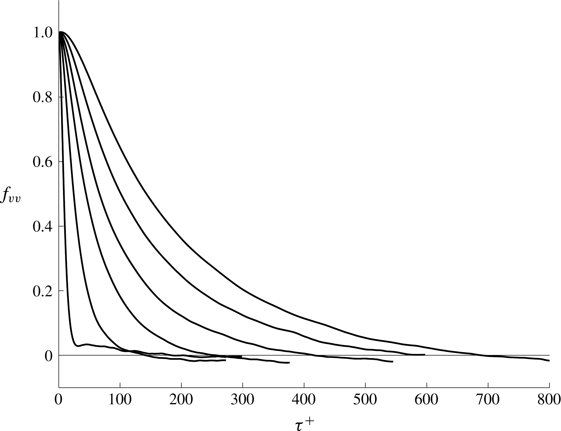
Using our ensembles of computed particle paths, the correlation functions $f_{vv}$ can be evaluated and from this an estimate of $T_{22}^{+}$ can be determined. Figure 11 shows the computed trends in $f_{vv}$ for $y^{+}\geqslant 31.2$ , while figure 12 has plots of $f_{vv}$ in the near-wall region $y^{+}\leqslant 14$ . Considering figure 11, it is seen that the correlation measured by $f_{vv}$ persists for longer times the further the ending plane of the paths is from the wall. The functions themselves display a smooth regularity apart from the curve closest to the boundary which has a slight maximum before decreasing to zero.

Figure 11.

The computed correlation coefficient $f_{vv}$ for paths arriving at $y^{+}=31.2$ , 121, 264, 452, 673, 914 (curves increase in magnitude and extent with $y^{+}$ , so the top curve is at  $y^{+}=914$ ).

Figure 12.

The computed correlation coefficient $f_{vv}$ for paths arriving at $y^{+}=1.9$ , 2.8, 3.8, 6.4, 14 (curves decrease in magnitude and extent as $y^{+}$ increases, so the top curve is at  $y^{+}=1.9$ ).

Near the wall, figure 12 shows a very much different story. Here, despite the use of large data sets, the $f_{vv}$ correlation is quite noisy, becomes noisier as the wall is approached and includes an increasingly large second maximum similar to that in the curve at $y^{+}=31.2$ in figure 11. The phenomenon at work in the near-wall region consists of a large and rapid drop off in correlation in a short time followed by a long period of noisy correlation. Evidently, this behaviour must reflect the idiosyncrasies of flow in the thin viscous region, where long-time correlations are produced in the velocity field by the passage of vortical structure overhead. Apparently, until enough individual events are sampled, the statistics will not be as smooth as they are at points further from the wall.

The area under the $f_{vv}$ curves is $T_{22}^{+}$ , which can be evaluated by numerical quadrature. The result is shown in figure 13(a) for the whole channel and in figure 13(b) as a close up of the near-wall region. Evidently, $T_{22}^{+}$ varies linearly throughout most of the channel, including the region from approximately $y^{+}=25$ to $y^{+}=900$ where it begins to level off, since it must be relatively constant at the centreline due to symmetry. Close to the wall, $T_{22}^{+}$ is as large as it is at the centreline, and it drops rapidly to its minimum near $y^{+}=15$ . The behaviour of $T_{22}^{+}$ is not unlike that of $\unicode[STIX]{x1D70F}_{D}^{+}$ shown in figure 7, although it is approximately $1/3$ as large in the central part of the channel.

Figure 13.

The behaviour of $T_{22}^{+}$ computed in channel flow: (a) across the channel; (b) close up of the near-wall region.

Our main interest in $T_{22}^{+}$ is in combination with $\overline{v^{2}}^{+}$ to form the physically correct eddy viscosity. This is shown plotted in figure 14 together with the distribution of eddy viscosity that is guaranteed to lead to an accurate calculation of $\overline{U}$ via a gradient Reynolds stress model, namely

(5.9) $$\begin{eqnarray}\unicode[STIX]{x1D708}_{T}=\frac{-\overline{uv}}{\text{d}\overline{U}/\text{d}y}.\end{eqnarray}$$

Any disagreement between these eddy viscosities reflects how $\unicode[STIX]{x1D708}_{T}$ in (5.9) is essentially covering up errors deriving from non-gradient physics included within the displacement and acceleration transport terms as well as slight non-zero values of $\overline{u_{b}v_{a}}$ . Figure 14(a), comparing (5.7) and (5.9), suggests that the most serious conflict in eddy viscosity occurs in the central region beyond $y^{+}=500$ , where the physical eddy viscosity is approximately constant and the modelled version decreases. In the immediate neighbourhood of $y^{+}=500$ , the exact and modelled eddy viscosities appear to be the same. Nearer the wall, the disagreement in eddy viscosities does not appear to be especially significant, although the closer look afforded by the log–log plot in figure 14(b) reveals some apparently small differences between the exact and modelled eddy viscosities that are both quantitative and qualitative.

Figure 14.

The eddy viscosity in channel flow: (a) comparison between ○, $T_{22}^{+}\,\overline{v^{2}}^{+}$ and ——, $\unicode[STIX]{x1D708}_{T}^{+}$ ; (b) log–log plot highlighting the near-wall behaviour.

To assess the impact that the differences in eddy viscosity have on how well gradient wall physics accounts for $\overline{uv}$ , figure 15 compares (5.4) with the Reynolds shear stress. This shows that the small differences in figure 14(b) actually mean that the physics of gradient transport is entirely unsuitable as a model of the near-wall Reynolds stress. In contrast, somewhat ironically, for $y^{+}\geqslant 400$ , the gradient model is generally a good fit where the greatest differences in eddy viscosity are observed in figure 14(a). The latter observation must reflect the fact that the mean velocity in the central region of the channel in not far removed from a linear variation, and the mixing lengths for points beyond $y^{+}=400$ are such that fluid particles largely remain within the linear mean velocity field during the mixing time.

Figure 15.

The inadequacy of gradient transport physics: ——, $\overline{uv}^{+}$ ; ○, $-T_{22}^{+}\overline{v^{2}}^{+}\text{d}\overline{U}^{+}/\text{d}y^{+}$ .

In the idealized case of homogeneous shear flow, where $\overline{U}(y)=Sy$ and $S=\text{d}\overline{U}/\text{d}y$ is a constant shearing everywhere, it may be inferred from (5.4) and (5.7) that

(5.10) $$\begin{eqnarray}\unicode[STIX]{x1D6F7}_{D}=-\overline{v^{2}}T_{22}\frac{\text{d}\overline{U}}{\text{d}y}\end{eqnarray}$$

is an exact asymptotic expression for $\unicode[STIX]{x1D6F7}_{D}$ for large $\unicode[STIX]{x1D70F}$ . Thus, unlike channel flow, where (4.1) holds for large times, the infinite extent of the linear mean field in homogeneous shear flow has the consequence of eliminating the factors that would ordinarily work to decorrelate the displacement correlation after it forms. Moreover, the constancy of the asymptotic value of $\unicode[STIX]{x1D6F7}_{D}$ means that the same is true of the acceleration term  $\unicode[STIX]{x1D6F7}_{A}$ . Thus, in this instance also, $\unicode[STIX]{x1D6F7}_{A}$ persists as a potentially non-zero constant at large  $\unicode[STIX]{x1D70F}$ , despite the randomization of fluid particle trajectories.

6 Significant events leading to transport

Unlike the normal Reynolds stresses, where all samples of the velocity fluctuation make contributions to the mean value, the Reynolds shear stress is composed of many offsetting plus and minus contributions. Consequently, the value of $\overline{uv}$ at any point in the flow depends on the imbalance between plus and minus realizations. The net value of the correlation can therefore be viewed as the end result of the action of a subset of the total collection of realizations. Based on this idea, it becomes possible to get a somewhat more precise view of the factors that produce Reynolds shear stress as well as each of the terms on the right-hand side of (2.7) evaluated at time  $\unicode[STIX]{x1D70F}_{D}$ .

To implement this analysis in the case of $\overline{u_{a}v_{a}}$ , we consider its value at a point in the lower half of the channel where it is negative. At such locations, events for which $u_{a}$ and $v_{a}$ have opposite sign take precedence over events where they have the same sign. The average $\overline{u_{a}v_{a}}$ is negative either because a decisive majority of events have oppositely signed pairs, or because a few very strong events tilt the average to be negative. A combination of both tendencies might also prevail. The ensembles of paths that have been computed afford an opportunity to investigate this question. Thus, for any $y^{+}$ value, we order the $N$ paths that contribute to each of the correlations in (2.7) from the smallest to the largest contributors depending on the sign of the correlation. For example, for $\overline{u_{a}v_{a}}$ in the lower channel half, the ranking is from the most positive to the most negative, as shown in figure 16(a) for the data at $y^{+}=54.8$ . Now, calculating partial sums $\sum _{i=1}^{n}u_{a}^{i}v_{a}^{i}$ , $n=1,2,\ldots ,N$ , as shown in figure 16(b), it can be seen that a point is reached, say $n=N_{0}$ , where the sums change sign from positive to negative. The collection of contributions for $n\geqslant N_{0}$ may be viewed as the reason why the correlation is negative, since the other contributions cancel out between plus and minus. The fraction of events that are responsible for the correlation, namely $(N-N_{0})/N$ , as well as the distribution of the magnitudes of the contributing subset of paths, reveals useful information about the origin of the Reynolds shear stress.

Figure 16.

Contributions to $\overline{u_{a}v_{a}}$ at $y^{+}=54.8$ from a data set consisting of 169 344 points in lower channel half: (a) individual contributions ranked from largest to smallest; (b) cumulative sum of contributions in (a), showing zero crossing at $N_{0}=136\,176$ .

Figure 17 is a plot for each of the terms in (2.7) of the fraction of events (e.g. $(N-N_{0})/N$ in the example corresponding to figure 16) at each $y^{+}$ position whose contribution is not cancelled by events with the opposite sign. It is seen in figure 17(a) that for a large portion of the channel, $\unicode[STIX]{x1D6F7}_{D}$ and $\overline{uv}$ follow a very similar trend in which approximately 20 % of events are responsible for their occurrence. The percentage for each of these rises towards 30 % at $y^{+}=15$ and drops towards zero for small  $y^{+}$ . As $y^{+}$ approaches the centreline, $\overline{u_{a}v_{a}}\rightarrow 0$ , as does the corresponding fraction of significant events shown in figure 17(a). The latter trend is due to the natural cancellation of plus and minus events that must take place as the centreline is reached in a symmetric flow field. In the near-wall region, as highlighted in figure 17(b), even though the Reynolds shear stress is rapidly dropping in magnitude towards zero at the wall from the peak it had at $y^{+}=40$ , this has no bearing on the frequency of events contributing to $\unicode[STIX]{x1D6F7}_{D}$ until very close to the wall, in fact, within $y^{+}=10$ . This suggests that throughout the near-wall region, outside the viscous sublayer, the drop off in $\overline{u_{a}v_{a}}$ is not due to a decrease in the number of Reynolds stress producing events, but rather to the size of their contributions. Within the viscous sublayer itself, the frequency of Reynolds stress producing events diminishes, and with this $\overline{u_{a}v_{a}}$ becomes very small. In the same vein, it can be anticipated that the decrease in the magnitude of correlations such as $\unicode[STIX]{x1D6F7}_{D}$ for $\unicode[STIX]{x1D70F}>\unicode[STIX]{x1D70F}_{D}$ can be attributed to a decrease in the number of events that maintain coherency with $v_{a}$ as the elapsed time increases. At the same time, the relatively slow relaxation of $\unicode[STIX]{x1D6F7}_{D}$ towards zero attests to the longevity of a small number of significant Reynolds stress producing events in the flow field.

Figure 17.

The fraction of points in the data ensembles that account for the local computed values of the terms in (2.7): ——,  $\overline{u_{a}v_{a}}$ ; ○,  $\unicode[STIX]{x1D6F7}_{D}$ ; ▵,  $(\unicode[STIX]{x1D6F7}_{A}+\overline{u_{b}v_{a}})$ ; (a) whole channel; (b) detail of the near-wall region.

The special importance of $\unicode[STIX]{x1D6F7}_{D}$ to the Reynolds shear stress is indirectly implied by the fact that $\unicode[STIX]{x1D6F7}_{A}$ and $\overline{u_{b}v_{a}}$ are non-zero only due to a comparatively small number of events in the flow field. Thus, in contrast to displacement transport, where it can be expected that at any time approximately one fifth of the domain contains sources of Reynolds stress correlation, the other terms are the result of an occasional somewhat rare event. In fact, for virtually the entire channel, considerably less than 1 % of events in the samples explain why $\unicode[STIX]{x1D6F7}_{A}$ and $\overline{u_{b}v_{a}}$ are non-zero. The conclusion may be reached that besides being the dominant factor leading to Reynolds stress, the events causing $\unicode[STIX]{x1D6F7}_{D}$ to be prominent must represent a far more common process throughout the flow field than that leading to $\unicode[STIX]{x1D6F7}_{A}$ and $\overline{u_{b}v_{a}}$ .

7 Upstream analysis

It is of some interest to consider the upstream statistics of fluid particles that travel over the time $\unicode[STIX]{x1D70F}_{D}^{+}$ to arrive at fixed $y^{+}$ planes. This kind of information is helpful for understanding the physics of transport and potentially for providing insights into accurately modelling the process. In this section, we consider the properties of all particles arriving at $y^{+}$ positions, while, in the next section, we look at statistics for the subset of paths that are most directly connected with the presence of the Reynolds shear stress.

Some basic attributes of the ensemble of particles that arrive at given $y^{+}$ locations at time $t^{+}$ can be gleaned from figures 18 and 19, containing scatter plots in the $x^{+},y^{+}$ plane of where the particles were located at the earlier time $t^{+}-\unicode[STIX]{x1D70F}_{D}^{+}$ . The first of these figures is for particles arriving at $y^{+}=2.8$ , 8.9, 54.8 and the second is for $y^{+}=163$ , 452, 832. The mixing times associated with these points are $\unicode[STIX]{x1D70F}_{D}^{+}=86.5$ , 12.7, 41.6, 154.0, 435.7, and 598.0 respectively. In each figure, the ending point of the particles is indicated by a circle at the $x^{+}=0$ position. The plots show that the streamwise extent of the particle ensembles is a strong function of the local mixing time. This explains the very short upstream region for the data at $y^{+}=8.9$ , which is where the mixing time is at a minimum. The shapes of the scatter plots largely reflect the fact that particles travelling from closer to the wall are slower, so their starting points are closer to the streamwise end point. The particles arriving at $y^{+}=2.8$ are mostly travelling from further away from the wall so are arrayed beyond this point.

Figure 18.

Side view in the $x^{+},y^{+}$ plane scatter plot of upstream particle positions at $t^{+}-\unicode[STIX]{x1D70F}_{D}^{+}$ arriving at $t^{+}$ : (a)  $y^{+}=2.8$ ; (b)  $y^{+}=8.9$ ; (c)  $y^{+}=54.8$ .

Figure 19.

Side view in the $x^{+},y^{+}$ plane scatter plot of upstream particle positions at $t^{+}-\unicode[STIX]{x1D70F}_{D}^{+}$ arriving at $t^{+}$ : (a)  $y^{+}=163$ ; (b)  $y^{+}=452$ ; (c)  $y^{+}=832$ .

Figure 19 shows that particles travel from an increasingly distant upstream region that spreads outward rapidly as the terminal $y^{+}$ point increases. For the particles arriving at $y^{+}=452$ and 832, many have started from beyond the centreline. This creates the hooked appearance of the particles. In all cases, the ensemble of particles includes many that originate from close to the lower wall surface. It is interesting to observe that for the $y^{+}=832$ location, particles originate from the entire extent of the channel from one wall to the other.

The upstream locations plotted in figures 18 and 19 are based on timings of the maximum contributions to displacement transport, so that they are reflective of the most coherent motions of dynamical significance in the flow. Clearly, these figures show that the Reynolds shear stress must ultimately be viewed as the result of actions covering a large region in space–time, particularly for the data in figure 19, where the particles travel thousands of $x^{+}$ units and several hundred $t^{+}$ units to make the maximum contribution to transport. According to the figure, the correlation between $u_{a}$ and $v_{a}$ at $y^{+}=832$ appears to have its origin in motions originating over five channel widths upstream. Even at $y^{+}=154$ , the correlation arises from particles travelling more than a channel width upstream. From this perspective, there appears to be little that is local about the Reynolds shear stress.

The lateral spread of particles in the ensembles is shown in figure 20 for ending points on the planes $y^{+}=2.8$ , 163 and 452. As expected, the distributions are symmetric in the spanwise direction. The shapes of the particle distributions reflect a bias towards the upstream direction, which is another indication of how the varying mean velocity differentially affects the motion of particles travelling from below versus above the final destination. Since the lateral motion of the particles can be viewed as the sum of many small steps, irrespective of their vertical positions in the channel, a Gaussian distribution in the initial path positions is not unexpected.

Figure 20.

Top view in the $x^{+}$ , $z^{+}$ plane of upstream positions at $t^{+}-\unicode[STIX]{x1D70F}_{D}^{+}$ of particles arriving at $t^{+}$ at (a)  $y^{+}=2.8$ , (b)  $y^{+}=163$ and (c)  $y^{+}=452$ .

The Kolmogorov–Smirnov (KS) test was used to examine the goodness-of-fit hypothesis that the upstream spanwise particles obey a Gaussian distribution. The KS test is based on the maximum difference between an empirical and a hypothetical cumulative distribution function (Massey Reference Massey1951). In the present case, a Gaussian distribution function was fitted to the initial $z$ positions of the particles which was then compared with the data. It was found that the Gaussian hypothesis is met with a confidence interval of 99 % for all $y^{+}$ levels, suggesting that the distribution of transverse particle positions is indeed Gaussian. Figure 21 illustrates at four $y^{+}$ positions the degree to which the computed upstream initial $z$ positions fit the form of a Gaussian cumulative distribution function.

Figure 21.

The cumulative distribution function (CDF) for upstream spanwise particle position (solid line) compared with the fitted Gaussian CDF (dashed line): (a)  $y^{+}=8.9$ ; (b)  $y^{+}=54.8$ ; (c)  $y^{+}=211$ ; (d)  $y^{+}=523$ .

The probability density functions in the $x$ and $y$ directions could not be reliably fitted to any common distributions. Nonetheless, it is informative to consider the mean of the $x_{b}$ data as well as the standard deviations of the $x_{b},y_{b},z_{b}$ data, as shown in figures 22(a) and 22(b) respectively. Apart from a small increase in the viscous sublayer, the mean of $x_{b}$ decreases linearly with $y^{+}$ until approximately $y^{+}=600$ , after which it is approximately constant at a value of the order of six channel widths upstream of the endpoint. The linear behaviour of the mean of $x_{b}$ appears to be consistent with the linearity of $\unicode[STIX]{x1D70F}_{D}^{+}$ over the same range as seen in figure 7(a) and occurs despite the changes in mean velocity over this portion of the channel. Figure 22(b) shows that the standard deviation of the upstream particle locations in all three directions also increases somewhat linearly until $y^{+}=600$ , after which the standard deviation is approximately constant in the wall-normal and spanwise directions and falls in the streamwise direction. The upstream dispersion of the particles is much larger in the streamwise direction than either of the other directions, with the latter becoming close to each other by the centreline. The decrease in standard deviation in the $x$ direction in figure 22(b) shows that there is less of a spread in initial $x$ position far from the wall, suggesting a reduced role for the slower moving particles originating close to the wall. The statistics in figure 22 imply that all points within the central channel core beyond $y^{+}=600$ share a similar transport physics that reflects a reduced influence of the solid boundaries.

Figure 22.

(a) The streamwise mean of particles arriving at $y^{+}$ planes over the mixing time  $\unicode[STIX]{x1D70F}_{D}$ . (b) The standard deviation of upstream particle locations: ——,  $x$ direction; – – –,  $y$ direction; — ⋅ —,  $z$ direction.

8 Modelling

To the extent that the decomposition in (2.7) is taken as a route towards developing a physical explanation for the Reynolds shear stress, then it is required to develop models for the phenomena described by the individual terms. In view of the previous discussions, it is clear that the most important facet of the Reynolds stress physics is that associated with the classical idea of displacement transport. Here, we will show using the channel flow path data accumulated in this study how a practical and self-consistent basis can be set up for evaluating displacement transport. Generalization of the approach to other flows should be possible. Less clear is how the small contribution to Reynolds stress from the remaining terms in (2.7) as shown in figure 10 may be modelled. Such an effort, not considered here, will require firming up of the connection between structural features of the flow and their influence on particle acceleration and the $\overline{u_{b}v_{a}}$ correlation.

To develop a model for $\overline{v_{a}(\overline{U}_{b}-\overline{U}_{a})}$ , it should be noted that this expression can be evaluated in the form of an ensemble average over $N$ particle paths via

(8.1) $$\begin{eqnarray}\overline{v_{a}(\overline{U}_{b}-\overline{U}_{a})}=\frac{1}{N}\mathop{\sum }_{i=1}^{N}v_{a}^{i}(\overline{U}_{b}^{i}-\overline{U}_{a}),\end{eqnarray}$$

where the superscript $i$ denotes the particular member of the ensemble. In view of our previous discussion, in which the members of the ensemble are ordered from plus to minus in magnitude, (8.1) can be written as

(8.2) $$\begin{eqnarray}\overline{v_{a}(\overline{U}_{b}-\overline{U}_{a})}(y)=\frac{1}{N}\left[\mathop{\sum }_{i=1}^{N_{0}}v_{a}^{i}(\overline{U}_{b}^{i}-\overline{U}_{a})+\mathop{\sum }_{i=N_{0}+1}^{N}v_{a}^{i}(\overline{U}_{b}^{i}-\overline{U}_{a})\right],\end{eqnarray}$$

where it is assumed that the first sum in this relation is over those contributions to the left-hand side that cancel out plus and minus, while the second sum contains those that are of one sign and together are responsible for the non-zero value of $\unicode[STIX]{x1D6F7}_{D}$ . With this understanding, (8.2) can be written as

(8.3) $$\begin{eqnarray}\overline{v_{a}(\overline{U}_{b}-\overline{U}_{a})}(y)=\frac{1}{N}\left[\mathop{\sum }_{i=N_{0}+1}^{N}v_{a}^{i}(\overline{U}_{b}^{i}-\overline{U}_{a})\right].\end{eqnarray}$$

The $N-N_{0}$ terms that remain in (8.3) have initial points of travel in the wall-normal direction, namely $y_{b}^{i}$ , that are either above or below $y$ . Letting $N_{B}$ be the number from below and $N_{T}$ be the number from above, then $N_{B}+N_{T}=N-N_{0}$ . The sum in (8.3) can now be divided into two separate sums of particles, one of which has $y_{b}^{i}<y$ and the other of which has $y_{b}^{i}>y$ . This results in

(8.4) $$\begin{eqnarray}\overline{v_{a}(\overline{U}_{b}-\overline{U}_{a})}(y)=\frac{1}{N}\left[\left(\mathop{\sum }_{i=1}^{N_{B}}v_{B}^{i}(\overline{U}_{b}^{i}-\overline{U}_{a})\right)+\left(\mathop{\sum }_{i=1}^{N_{T}}v_{T}^{i}(\overline{U}_{b}^{i}-\overline{U}_{a})\right)\right],\end{eqnarray}$$

where now $v_{B}^{i}$ and $v_{T}^{i}$ respectively refer to the values of $v_{a}^{i}$ for particles originating below and above  $y$ . It is also assumed here that the index $i$ is reset to be $1\leqslant i\leqslant N_{B}$ and $1\leqslant i\leqslant N_{T}$ respectively for the two sets of particles. The two summations within parentheses on the right-hand side of (8.4) represent averages over the subensembles of points coming from below and above the destination point. The ratios $N_{B}/N$ and $N_{T}/N$ add up to the ratio $(N-N_{0})/N$ that was discussed in § 6 and plotted in figure 17.

Since $\overline{U}_{b}$ depends only on $y$ , a simplification of (8.4) can be had by organizing the elements of each of the two subensembles of paths according to their values of $y_{b}^{i}$ . For convenience, we refer to these $y$ values as being in the ensembles $y_{B}^{i}$ , $i=1,\ldots ,N_{B}$ , and $y_{T}^{i}$ , $i=1,\ldots ,N_{T}$ . Figure 23 is a scatter plot of $y_{b}^{i}$ , $v_{a}^{i}$ values for the data at $y^{+}=211$ that is representative of all points in the channel. Points travelling from below the final point are seen to all arrive at the final plane with positive values of $v_{a}$ and those travelling from above invariably have negative $v_{a}$ values. Clearly, paths for which travel to or from the wall is uninterrupted over the mixing time are favoured in contributing to the Reynolds shear stress.

Figure 23.

Scatter plot of $y_{b},v_{a}$ values for particles from the subensembles of significant contributors to $\overline{uv}$ arriving at $y^{+}=211$ .

Now, we consider the set of particles coming from below the final plane. The upstream values lie between

(8.5) $$\begin{eqnarray}y_{B}^{min}\equiv \min (y_{B}^{i},i=1,\ldots ,N_{B})\end{eqnarray}$$

and

(8.6) $$\begin{eqnarray}y_{B}^{max}\equiv \max (y_{B}^{i},i=1,\ldots ,N_{B}).\end{eqnarray}$$

We divide the region $y_{B}^{min}\leqslant y\leqslant y_{B}^{max}$ into $K$ equal subdivisions of length $\unicode[STIX]{x0394}y^{\prime }$ , with $y_{k}^{\prime }$ being the centre of the $k$ th box. Let $N_{B}^{k}$ be the number of particles for which $y_{b}^{i}$ is in the $k$ th box and let $p_{B}^{k}=N_{B}^{k}/N_{B}$ be the fraction of the $N_{B}$ particles initiating in the $k$ th subdivision where $\sum _{k}N_{B}^{k}=N_{B}$ . We define

(8.7) $$\begin{eqnarray}c_{B}^{k}=p_{B}^{k}/\unicode[STIX]{x0394}y^{\prime }\end{eqnarray}$$

as the concentration of particles in the $k$ th box. Let $\overline{v}_{B}^{k}$ be the average of the $v_{b}^{i}$ velocities in the $k$ th box. Using these definitions, the first term on the right-hand side of (8.4) becomes

(8.8) $$\begin{eqnarray}\displaystyle \frac{1}{N}\mathop{\sum }_{i=1}^{N_{B}}v_{B}^{i}(\overline{U}_{b}^{i}-\overline{U}_{a}) & = & \displaystyle \frac{1}{N}\mathop{\sum }_{k=1}^{K}\left(\mathop{\sum }_{i=1}^{N_{B}^{k}}v_{B}^{i}(\overline{U}(y_{k}^{\prime })-\overline{U}(y))\right)\nonumber\\ \displaystyle & = & \displaystyle \frac{1}{N}\mathop{\sum }_{k=1}^{K}N_{B}^{k}\overline{v}_{B}^{k}(\overline{U}(y_{k}^{\prime })-\overline{U}(y))\nonumber\\ \displaystyle & = & \displaystyle \frac{N_{B}}{N}\mathop{\sum }_{k=1}^{K}c_{B}^{k}\overline{v}_{B}^{k}(\overline{U}(y_{k}^{\prime })-\overline{U}(y))\unicode[STIX]{x0394}y^{\prime }.\end{eqnarray}$$

The relative importance of $N_{B}/N$ and $N_{T}/N$ divides the result in figure 17 into fractions from above and below that change with  $y$ . Then, we define

(8.9a,b ) $$\begin{eqnarray}\unicode[STIX]{x1D6FC}_{B}(y)=\frac{N_{B}}{N},\quad \unicode[STIX]{x1D6FC}_{T}(y)=\frac{N_{T}}{N}.\end{eqnarray}$$

Using (8.9) in the last expression of (8.8) and taking the limit as $\unicode[STIX]{x0394}y^{\prime }\rightarrow 0$ , we obtain the integral

(8.10) $$\begin{eqnarray}\unicode[STIX]{x1D6FC}_{B}(y)\int c_{B}(y,y^{\prime })\overline{v}_{B}(y,y^{\prime })(\overline{U}(y^{\prime })-\overline{U}(y))\,\text{d}y^{\prime },\end{eqnarray}$$

where the integration limit is from one wall of the channel to the other.

Use of a similar analysis of the contributions to the displacement transport term coming from particles originating above the destination plane leads to an expression equivalent to (8.10) and containing $\unicode[STIX]{x1D6FC}_{T}(y)$ , $\overline{v}_{T}(y,y^{\prime })$ and $c_{T}(y,y^{\prime })$ . From these results, the derived model for the displacement transport term is

(8.11) $$\begin{eqnarray}\overline{v_{a}(\overline{U}_{b}-\overline{U}_{a})}=\int _{0}^{h}F(y,y^{\prime })(\overline{U}(y^{\prime })-\overline{U}(y))\,\text{d}y^{\prime },\end{eqnarray}$$

where the kernel function is

(8.12) $$\begin{eqnarray}F(y,y^{\prime })=\unicode[STIX]{x1D6FC}_{B}(y)c_{B}(y,y^{\prime })\overline{v}_{B}(y,y^{\prime })+\unicode[STIX]{x1D6FC}_{T}(y)c_{T}(y,y^{\prime })\overline{v}_{T}(y,y^{\prime }).\end{eqnarray}$$

At any given $y$ location in the channel, (8.11) shows how the displacement transport term arises from fluid particles travelling from different $y^{\prime }$ positions. This relation takes advantage of the streamwise uniformity in channel flow to develop a compact formula. In more general situations, it can be expected that the potentially significant upstream origin of the particles arriving at destination points would have to be taken into account in deriving formulae similar to (8.12).

Figure 24.

Contour plot of $F(y^{+},y^{\prime ^{+}})$ in the lower half channel. Solid lines are positive values and dashed lines are negative values.

The most essential part of the physics behind the Reynolds shear stress is contained in the function $F(y,y^{\prime })$ . To determine it numerically, its values on the 23 $y^{+}$ locations where particle data were obtained were computed and then these values were interpolated into a square mesh covering the lower half channel. A numerical calculation shows that the computed $F(y,y^{\prime })$ is fully self-consistent with (8.11). A holistic view of $F(y^{+},y^{\prime ^{+}})$ for the lower channel half is shown in figure 24, which puts into sharp focus the intrinsic non-locality of the mechanism responsible for the Reynolds shear stress. Taken as a whole, figure 24 calls into question the relevance of the local mean velocity derivative in determining displacement transport.

Near the wall, the peak contributions to the local displacement transport at a particular point come from fluid particles that originate at points offset immediately to either side of the point in question. The peaks move apart with increasing distance from the wall, creating a growing separation between the influences of particles travelling from below and above the destination point. Figure 25 is a plot of the $y^{\prime ^{+}}$ dependence of $F(y^{+},y^{\prime ^{+}})$ at the three locations $y^{+}=35.3$ , 211.7 and 329.2. The plots show how the peak positive contributions rapidly decrease in magnitude with distance from the wall, reflecting the spreading out of the region of influence on $\unicode[STIX]{x1D6F7}_{D}$ of initial particle locations. The increasing extent of the region centred on each $y^{+}$ location from which particles contributing to displacement transport do not originate is apparent. According to figure 24, such a region first develops at $y^{+}\approx 100$ and increases significantly with distance from the wall. This trend appears to call into question the appropriateness of a local dependence of the Reynolds shear stress on the mean velocity gradient, even in the region away from the wall seen in figure 15 where a gradient model seems to be justified. However, there is an implicit dependence of $\unicode[STIX]{x1D6F7}_{D}$ on the mean gradient over the mixing time in the difference between mean velocities in (8.11). This is made particularly clear in the case of homogeneous shear flow, where (5.10) applies. For channel flow and presumably for flows encountered in engineering practice, the implication of (8.11) is that gradient transport is not an appropriate means of accounting for the full effect of displacement transport.

Figure 25.

Plot of $F(y^{+},y^{\prime ^{+}})$ for the $y^{+}$ values (a) 35.3, (b) 211.7 and (c) 329.2.