INTRODUCTION
Beef production from females (adult cows and heifers) ranges from 0·32 to 0·88 of slaughtered cattle in Europe (not counting calves) (Cabaraux et al. Reference Cabaraux, Dufrasne, Roux, Istasse and Hornick2005), which corresponds to one-third of beef consumption in Europe. France is the country with the highest proportion of beef consumption from adult females (beef and dairy), about 0·80. Farm income from the sale of finished cull cows (up to 3 years old) constitutes an important component of the total output and is about 0·10 in dairy farms (Veysset, personal communication, data 2004–2005) and 0·30 in beef farms. This proportion varies in suckler herds according to the area and breed, ranging from 0·17 for Salers herds (Massif Central, France) to 0·26 and 0·30 in Charolais and Limousin, respectively (Lherm, personal communication, data 2002–2005).
Farm observations in France highlight a wide phenotypic variability in cull cows of the same breed, finished or not (Bastien & Brouard-Jabet Reference Bastien and Brouard-Jabet2000; Pierret et al. Reference Pierret, Breuvart and Eisenzaemmer2002, Reference Pierret, El-Omari and Dumont2004). Age, frame size, physiological status (dry or lactating cow, pregnant or non pregnant), health status and body condition of cull cows at the beginning of finishing are very variable and constitute the factors modifying their finishing ability. Finishing diets are also very variable, with diets of contrasting energy concentration. Finishing can occur indoors with diets including hay, maize silage or very high proportions of concentrate. Cows can also be finished by grazing on high quality pastures.
Farmers can alter carcass composition, proportion of intramuscular fat and meat colour through farming practices, feeding level and nature of the diet. Previous INRA nutritional recommendations (Geay & Micol Reference Geay, Micol and Jarrige1988) for culled cows during finishing were based on live weight, live weight gain and the beef or dairy breed characteristics. They were formulated using the experimental data available, considering the direct relationship between live weight gain, and energy and protein supply without taking into account the mechanistic processes (contrary to the factorial method used for growing and finishing young cattle; Geay et al. Reference Geay, Micol, Robelin, Berge and Malterre1987). Consequently, these recommendations do not consider major factors such as body condition and age. To update the recommendations (Garcia et al. Reference Garcia, Agabriel and Micol2007) for culled cows during finishing, a predictive model of the energy requirements was developed allowing for all the available on-farm information.
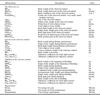
The overall approach used the equations developed by Robelin & Daenicke (Reference Robelin and Daenicke1980) for young cattle and used the classic factorial method that sums the maintenance requirements (digestive metabolism, cell turnover and body temperature regulation) and the requirements associated with live weight gain, that is, the sum of the energy in lipid and protein (Bruce et al. Reference Bruce, Broadbent and Topps1984; Vermorel et al. Reference Vermorel, Coulon and Journet1987; Williams & Jenkins Reference Williams and Jenkins2003a, Reference Williams and Jenkinsb). The present paper describes this model, called CompoCow (Table 1), its principal components and hypotheses, the calibration, sensitivity analysis and then an initial validation with experimental data.
List of abbreviations of variables for growth and finishing of the reference animal, application to the observed animal and estimation of requirements

fin=finisher.
MODEL DESCRIPTION
CompoCow calculates the energy requirements of an observed culled cow during its finishing. For this purpose, it sums the energy requirements for maintenance and the energy requirements for live weight gain as described by Bruce et al. (Reference Bruce, Broadbent and Topps1984), Williams & Jenkins (Reference Williams and Jenkins2003a, Reference Williams and Jenkinsb) and many others.
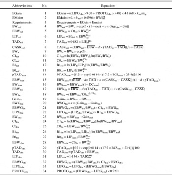
The model estimates the composition of gain in cull cows in terms of lipid and protein deposition, and the associated energy requirement during finishing (Eqn 1, Table 2). The model includes the effects of age, live weight, the body condition of the animal and the level of growth on the composition of gain. It also takes into account that live weight varies according to development and finishing and considers that gain due to growth is achieved without change in body composition. The lipid proportion of live weight gain increases during finishing, whereas protein and water content decreases, which results in a higher energy content of gain. The model of body composition evolution for cows is the basis of CompoCow, characterized by the following four main features:
(i) CompoCow incorporates a growth model for lifetime performance and a finishing model for finishing period to allow for the effects of age and frame size on composition of weight gain.
(ii) CompoCow relies on Gompertz and monomolecular equations to describe the evolution of live weight against time, growth and then finishing.
(iii) CompoCow utilizes allometric equations to estimate body composition over time from the growth curves mentioned above.
(iv) The derived equations for growth curves and for the allometric relationships estimate the gain and composition of gain in terms of lipid and protein.
Equations of the CompoCow model

Maintenance requirements are calculated as a function of metabolic weight (BW0·75), according to Eqn (2) (Table 2). The figure 0·4396 in Eqn (2) corresponds to the maintenance requirements of a dry cow in Million Joules (MJ) of metabolizable energy (ME)/kg of metabolic weight (Petit Reference Petit and Jarrige1988). The parameter λ allows for the effects of farm management issues such as stalls, feeding level and body condition score (BCS). The k g and k mf coefficients correspond respectively to the efficiencies of transformation of ME into net energy (NE) for tissue growth and for both maintenance and production within the INRA energy system (INRA Reference Jarrige1989).
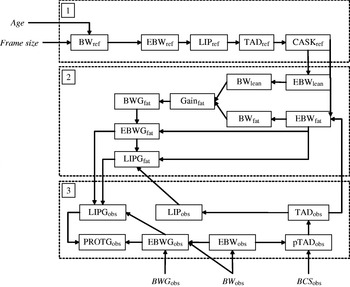
CompoCow calculates the composition of gain in terms of lipid and protein (LIPGobs, PROTGobs) according to three sub-models described in Figs 1 and 2:
(i) A model that estimates the body weight (BW) and composition of a reference animal of the same age and frame size as the observed cow, during its lifetime performance (Fig. 1, Frame 1, and Fig. 2a).
(ii) A model that estimates the evolution of live weight and composition of this reference animal during finishing (Fig. 1, Frame 2, and Fig. 2b).
(iii) A model that estimates the composition of gain of the observed cow and its associated requirements, from the results obtained with the reference animal.
Simplified structure of the CompoCow model, not showing the calculation and utilization of allometry coefficients. Frame 1 corresponds to the growth model for the reference animal. Frame 2 shows the finishing model for the reference animal and frame 3 corresponds to the application of the model to the observed cow. Variables outside the frames correspond to the inputs to the model.

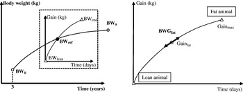
Growth model (bold line) and finishing model (dashed frame) for the reference animal. The graph on the left shows both models with growth from BW at 3 years old (BW0) to BW at maturity (BWa) according to a growth curve of reference BW (BWref) as a function of age in years. The graph on the right side focuses on the finishing model (in dashed frame on the left) with weight gain from a lean BW (BWlean) to a maximum BW at the end of finishing (BWend), as a function of a finishing duration in days.

CompoCow uses as inputs the age of the observed animal (Ageobs), its live weight (BWobs), its BCS (BCSobs measured on a scale from 0·5 to 5), frame size (three possibilities) and the target for daily live weight gain (BWGobs).
Model of the reference cow during its lifetime performance
The model of growth of the reference animal estimates BW (BWref) from the initial BW (BW0) at 3 years old to BW at maturity (BWa) according to a Gompertz equation as a function of age in years (Eqn 4, Table 2). Additional equations (Eqns 5–8, Table 2) are used to estimate the corresponding body composition in terms of empty BW (EBWref), body lipid (LIPref), total adipose tissue (TADref) and carcass skeleton weight (CASKref: bone content of the carcass). This model considers that the reference animal is characterized by the same age and the same frame size as the observed cow.
Model of the reference cow during finishing
The lipid deposition model for the reference animal estimates daily BW gain (BWGfin), according to Eqn (20)(Table 2), as a function of the theoretical BWG made from the lean to the actual status (Gainfin). The experimental data available to estimate the parameters of Eqn (20) referred to its integral, i.e. Eqn (A1). Consequently, Eqn (A1) was fitted, which calculates BW (BWfin) during finishing according to the following monomolecular equation:

BW goes from a lean BW at the beginning of finishing (BWlean) to a maximal BW at the end of finishing (BWend). Gainend (kg) is the maximal weight gain that could be achieved at the end of finishing. Duration is the length of the finishing period (in days) and r is the constant rate of daily body gain decrease.
To estimate BWGfin, the model first calculates Gainfin by difference between BW for the lean animal (BWlean) having standard carcass skeleton (CASKref) and its BW (BWfin) when it exhibits the same quantity of total adipose tissue as the observed cow (Eqn 19). Additional equations (Eqns 21 and 22) were then applied to estimate the corresponding empty BWG (EBWGfin) and the lipid gain (LIPGfin).
Application to the observed cow
CompoCow calculates the characteristics of the reference cow during growth using age and frame size of the observed cow (Frame 1, Fig. 1). It then estimates the evolution of BW and body composition of this reference animal during finishing. The reference animal during finishing is characterized by the same quantity of total adipose tissue and of body lipid as the observed cow (arrow from TADobs to EBWfin between frame 3 and frame 2, Fig. 1). BWG and BWG composition for the reference cow are calculated by difference with the lean state of the reference cow at the beginning of finishing. The model considers that the observed cow is characterized by BW composition and by BWG composition similar to the reference animal of the same status (age and frame size). Consequently, the lipid gain of the reference animal is converted for the observed cow according to Eqn (33) (Table 2), which moderates the lipid gain for the reference animal with the ratio between the empty body gain of the observed and the reference animals.
Prediction of body composition using CompoCow
Prediction of body composition corresponds here to estimation of empty BW, body lipid weight and carcass skeleton weight (CASK). Allometric equations established by Robelin & Daenicke (Reference Robelin and Daenicke1980) were used to estimate empty BW and body lipid weight of the reference cow (Eqns 5 and 6, Table 2) and empty BW of the observed cow (Eqn 28). The corresponding derived equations are used to calculate the empty BWG and the body lipid gain of the reference cow (Eqns 21 and 22) and the empty BWG of the observed cow (Eqn 32).
These equations were applied at 3 years old and at maturity for the growth model to calculate the allometric coefficients C0ref, C1ref, B0ref and B1ref (Eqns 10–13, Table 2). The allometric equation for empty BW is applied at the beginning and at the end of finishing to calculate C0fin and C1fin (Eqns 24 and 25, Table 2). The allometric equation for lipid was applied at the beginning of finishing and at the reference animal BW (BWfin) to calculate B0fin and B1fin (Eqns 26 and 27, Table 2). The model then calculates body composition and composition of gain at any place along the growth curves.
CASK is an indicator of frame size and is calculated using an equation relating empty BW to total adipose tissue weight and CASK (Eqns 15 and 17, Table 2). In the overall model, it is assumed that the CASK does not change during finishing. This equation is used to calculate CASKref (Eqn 8), EBWlean (Eqn 15) and EBWfin (Eqn 17).
Additional equations are used to convert BCS into body lipid contents. For this purpose the following were used: (i) an equation that links the content of total adipose tissue in empty BW (TAD_EBW) to BCS (Eqn 29, Agabriel et al. Reference Agabriel, Giraud and Petit1986 and personal communication) and (ii) an equation that links total adipose tissue weight to body lipid weight (Eqn 31, Geay et al. Reference Geay, Micol, Robelin, Berge and Malterre1987).
MATERIALS AND METHODS
Datasets used to develop equations and to challenge the model
Calibration and testing of the model were performed with several datasets taken from published experiments, on-farm measurements and slaughter measurements:
• Dataset 1 utilizes data from the INRA experimental farms Laqueuille, Marcenat and Theix. This dataset includes data on BW, height at the withers (indicator of frame size), BCS and age of Charolais (n=11 072), Limousine (n=4790) and Holstein (n=2470) cows during their lifetime performance.
• Dataset 2 includes data from the experimental slaughterhouse at Theix, which includes CASKs, total adipose tissues and empty BWs of slaughtered Charolais (n=127), Limousine (n=111) and Holstein (n=168) cows.
• Dataset 3 a was developed from published and unpublished experiments conducted at INRA experimental farms, which included data on the dynamics of finishing, i.e. data on BW according to finishing duration, for 13 groups of Charolais cows (Dumont et al. Reference Dumont, Roux, Agabriel, Touraille, Bonnemaire, Malterre and Robelin1991; Roux et al. Reference Roux, Dumont, Agabriel, Bonnemaire and Micol1993; Agabriel et al., personal communication) and five groups of Holstein cows (De La Torre et al. Reference De La Torre, Gruffat, Durand, Micol, Peyron, Scislowski and Bauchart2006; Berge et al., personal communication). This dataset was used for model calibration.
• Dataset 3b included data from published experiments conducted at INRA experimental farms. It contained information on the average age, BW, BCS, BWG and NE intake of 31 groups of Charolais cows (Dumont et al. Reference Dumont, Roux, Agabriel, Touraille, Bonnemaire, Malterre and Robelin1991, Reference Dumont, Roux, Touraille, Agabriel and Micol1997; Roux et al. Reference Roux, Dumont, Agabriel, Bonnemaire and Micol1993). This dataset was used for the purpose of validating the model.
Calibration of model parameters
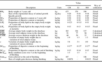
CompoCow was parameterized for Charolais, Limousine and Holstein breeds (Table 3) by using two different methodologies:
(i) The literature and expert knowledge were used for body composition at the beginning and at the end of both growth and finishing phases.
(ii) Experimental data were used to develop relationships between weight, body condition and frame size, and also for BW change during lifetime performance and during finishing.
Description, units, value and way of estimating parameters of the model applied to Charolais (CH), Limousin (LI) and Holstein (HO) cows

* Average value for a cow at 5 years olds.
Digestive content during the breeding life (DC0 and DCa) was estimated from expert knowledge and literature data (INRA Reference Jarrige1989; Agabriel et al. Reference Agabriel, Petit and Giraud1993), and was set to a proportion of 0·20 at 3 years old and 0·22 for mature cows (see Table 3). These values resulted from rumen contents (that represent 0·80 of the gut fill; Béranger & Robelin Reference Beranger and Robelin1978) measured on Charolais rumen-fistulated cows fed with a restricted hay diet (14·5 kg dry matter). This type of diet corresponds to the usual diet of the Charolais and Limousin cows on the INRA experimental farm during winter. Digestive content in Limousin cows was set at 0·18–0·20, which corresponds to about 0·90 of the digestive content in Charolais or Holstein cows, to account for the lower intake capacity of Limousin cows (Petit et al. Reference Petit, Garel, D'Hour, Agabriel, Journet, Grenet, Farce, Theriez and Demarquilly1995). Digestive content at the beginning (DClean) and at the end (DCend) of finishing were set to 0·85 and 0·75 of DC0, respectively, using data from the experimental farms Laqueuille (Massif Central, France) and Le Pin (Normandy, France). The decrease in digestive content relative to breeding life accounts for the lower fill effect of high concentrate diets during finishing.
The proportion of lipid in the empty BW at 3 years old (0·125, LIP0) and at maturity (0·13, LIPa) in Charolais cows corresponded to the average values of BCS (2·5 over 5) calculated from the dataset for the experimental farm Laqueuille (Dataset 1) (Table 3). As Limousin cows tend to accumulate more lipid in subcutaneous fat than Charolais cows (Robelin et al. Reference Robelin, Agabriel, Malterre and Bonnemaire1990), lower lipid proportions for young Limousin cows than for Charolais were considered. Lipid proportions during lifetime performance were set lower for Holstein cows considering a BCS of 2 over 5, consistent with the experimental database. Indeed, Holstein cows exhibit a lower average body score than Limousin and Charolais cows, due to greater use of body lipid for lactation. BCS at the beginning of finishing corresponds to lean body condition. BCSlean at 1·5 was set for suckler cows (in the present case Charolais and Limousin) and at 1·0 for dairy cows from published experimental data (Jones Reference Jones1983; Malterre et al. Reference Malterre, Robelin, Agabriel and Bordes1989; Agabriel et al. Reference Agabriel, Garel, Lassalas and Petit1991; Dumont et al. Reference Dumont, Roux, Agabriel, Touraille, Bonnemaire, Malterre and Robelin1991, Reference Dumont, Roux, Touraille, Agabriel and Micol1997; Roux et al. Reference Roux, Dumont, Agabriel, Bonnemaire and Micol1993).
Fitted parameters corresponded to the equations that estimate BW during lifetime performance (BWref), daily gain during finishing (BWGfin) and the relationship between empty BW, total adipose tissue and carcass skeleton. Parameters BW0, a and b of Eqn (4) were fitted using PROC NLIN (SAS Institute Inc. 1999) with 11 072 weight measurements of Charolais, Limousin and Holstein cows (Dataset 1). Parameters Gainend and r of Eqn (A1) were fitted using weight measurements of cull cow groups during finishing (13 groups of Charolais cows and 5 groups of Holstein cows, Dataset 3a). Fitting in this case was performed with PROC NLMIXED (SAS Institute Inc. 1999) to account for the random effect of each group.
The equation for prediction of CASK (Eqn 8) was calibrated with Dataset 2. Parameters  ,
 and
 were calculated for Charolais, Limousin and Holstein cows as the average values for the dataset from the experimental slaughterhouse at Theix. The equation was then fitted with PROC NLIN (SAS Institute Inc. 1999) to estimate parameters d and o.
To account for the variability in frame size at maturity, three levels of frame size were defined, i.e. small, medium and large. These levels were defined considering the variability in height at the withers observed in Dataset 1. First an equation was fitted relating BW to height at the withers (WH) and BCS:

 ,
 and
 are the average values in Dataset 1 for BW, WH and BCS, respectively, used to fit parameters h and n. Next, standard deviation around the average WH was used to define the frame sizes. Average value plus two standard deviations corresponds to large frame size, average value corresponds to medium frame size and average value minus two standard deviations corresponds to small frame size. Multiplying the standard deviation by the h parameter gives the modification in BW obtained when changing the frame size category. The values of BW at maturity were modified using this factor and the values obtained were divided by exp(b) to obtain different values of BW0 for small, medium and large cows.
Sensitivity analysis
A sensitivity analysis was performed on the model in order (i) to investigate the model's behaviour and check that it simulates correctly the hypotheses that were included and (ii) to identify the inputs and parameters to which the model is most sensitive for further calibration. Indeed, knowledge of model sensitivity gives insights into the level of precision needed to parameterize a model.
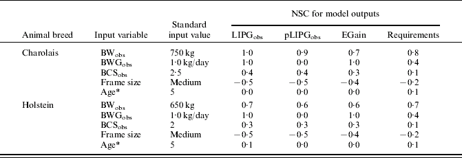
Sensitivity analysis was performed in two steps: first, an overall approach that consisted of assessing the influence of the input values (BWobs, BCSobs, BWGobs and frame size) on the output values through the normalized sensitivity coefficient (NSC). Output values that were investigated included the proportion of lipid in empty body gain (pLIPGobs), the quantity of lipid in the gain (LIPGobs), the resulting energy for gain, and the requirements. As described in Jouven et al. (Reference Jouven, Agabriel and Baumont2008), NSC corresponds to the ratio of the rate of variation of the output variable to the rate of variation of the input value tested. The level of NSC indicated whether the sensitivity of the model to the parameters should be evaluated at constant input values (in the case of a high degree of sensitivity to inputs) or at variable input values.
Next, the analysis was focused on sensitivity to the parameters. NSC coefficients for the parameters were calculated, considering the outputs pLIPGobs, LIPGobs, EGain and the requirements. The analysis was completed by performing response surface analysis as described in Ruget et al. (Reference Ruget, Brisson, Delecolle and Faivre2002) to investigate possible cross-effects of the parameters on the LIPGobs output variable. Response surface methodology consists of fitting a surface (of dimension n+1, if n parameters are studied) that corresponds to the response of the model to the parameters. The surface was fitted according to a second order equation, with cross and quadratic terms, by using PROC RSREG (SAS Institute Inc. 1999):

In the above equation, x i corresponds to the parameters, x ix j are the cross terms and x ii2 are the quadratic terms. The β coefficients of the regression estimate the model response. The variation rate of the parameters was set to±10%, except for BW0 where it was set to±5% to avoid values of BW0 that would correspond to another frame size. Parameters d and o of Eqn (8) were not subjected to sensitivity analysis as they are not involved in the dynamic processes of growth or finishing.
LIPGobs and the NE for gain are expected to be highly sensitive to the input value for BWGobs, whereas pLIPGobs is expected to be more sensitive to the observed condition score. Requirements should be highly sensitive to the BWGobs but also to BWobs, because maintenance requirements represent about two-thirds of total requirements. Sensitivity analysis for pLIPGobs and LIPGobs is useful to investigate the consistency between the assumptions and the behaviour of the model.
Application to a Charolais cow dataset
The CompoCow model was tested with a dataset of 31 groups of Charolais cows finished in the INRA experimental farms (Dataset 3 b). Selected groups were characterized by data including average values for the finishing period of BWobs, BWGobs, BCSobs, Ageobs and NE intake. Average characteristics of the animals in the dataset were: Ageobs=5·6±1·33 years, BWobs=684±48·9 kg, BCSobs=2·6±0·31, finishing duration=80±24·7 days and BWGobs=1·3±0·23 kg/day. Initial BCS was 1·8 on average and animals were slaughtered at a target BCS of 3·5 over 5. Total NE requirements estimated by the model, energy for gain plus energy for maintenance were compared with the NE intake of the groups to achieve the observed gain. The parameter λ for maintenance requirements was fitted to minimize the sum of squares of the difference between observed and estimated total requirements. A synthetic approach was used as described in Offner & Sauvant (Reference Offner and Sauvant2004) that consists of estimating the mean bias, the regression slope of the observed values against the predicted values, the root mean squared deviation and the coefficient of determination (r 2). The distribution of residuals was studied against the predicted values and against several input values (BWobs, BCSobs, BWGobs, etc.) to identify any possible bias. The same evaluation was performed with the previous recommendations (INRA Reference Jarrige1989) to quantify the improvements obtained with CompoCow.
RESULTS
Behaviour of the model
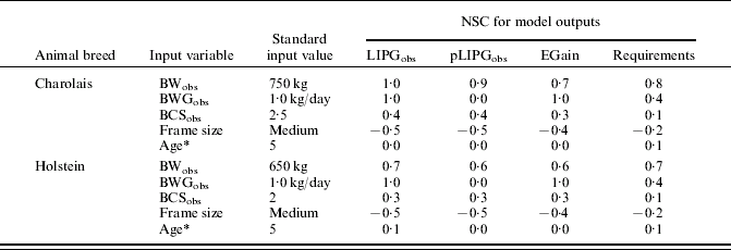
Table 4 shows the values of NSCs for four outputs of the CompoCow model: LIPGobs, pLIPGobs, EGain and Requirements. Results highlight for both Charolais and Holstein cow calibrations that the composition of gain, i.e. pLIPGobs, and the level of lipid gain are sensitive to the BW, BCS and frame size that are attributed to the observed cow. Higher sensitivity is obtained with BWobs for which NSC of LIPGobs and pLIPGobs are respectively 1·0 and 0·9 for Charolais cows. Consequently, these inputs strongly influence the level of NE for gain. BWobs also alters the total requirements because of its impact on both energy for gain and energy for maintenance, whereas BCSobs and frame size mainly modify the energy for gain. Sensitivity of the model to BWobs is lower for the Holstein cow calibration than for the Charolais cow calibration, because levels of lipid gain are already close to the maximum, i.e. empty BWG, in the Holstein cow calibration. The NSCs concerning observed BWG are quite high for LIPGobs, EGain and the requirements. However, BWGobs has no impact on the composition of gain as the NSC for pLIPGobs is nil. Sensitivity of the model to the age of the animal was calculated as though the observed animal has the same characteristics as the reference animal described in the growth model. This was done to avoid confounding the strong interactions of age with the difference between BWobs and BWref. Sensitivity of the model to age of the observed animal was very low, and even negligible for composition of gain and energy for gain, which can be explained by the fact that the finishing model is the same whatever the age.
Normalized sensitivity coefficients (NSC=ratio of the rates of variation of the output to the input) of the CompoCow model to the input values (with a±20% of variation), for the Charolais and Holstein calibrations. Output variables investigated are the proportion of lipid in empty body gain (pLIPGobs), level of lipid gain (LIPGobs), NE for gain and total requirement. Sensitivity to frame size is calculated by increasing the standard frame size to the large category and decreasing it to the small category
* NSC has been calculated for an observed animal that has the same characteristics as the reference animal.
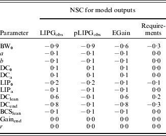
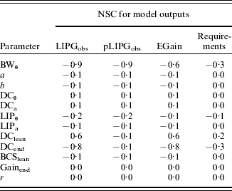
From the results in Table 4, it was deduced that the sensitivity of the model to the input values is quite high. Consequently, the sensitivity of the model to the parameters was analysed for the standard input values in Table 4. Table 5 shows the NSCs of the model for a±20% variation in the parameters for the Charolais cow calibration. The model is mainly sensitive to the parameters BW0, DClean and DCend. The LIPGobs, pLIPGobs, EGain and animal requirements decrease when BW0 increases. The digestive content at the end of the finishing period modulates the level of empty body gain, and consequently of LIPobs, EGain and the requirements but has little impact on the composition of gain. The higher the digestive content at the end of finishing, the lower the empty body gain estimated for the observed animal. On the contrary, the higher the digestive content of the lean animal, the higher the empty body gain of the observed animal, and consequently LIPGobs, EGain and the requirements. It is interesting to note that the parameters of the body gain curve during finishing have no impact on the main outputs of the model, as NSCs are nil. Indeed, when only Gainend and/or r are modified in the model, LIPGobs and pLIPGobs do not change because LIPGobs is a function of the ratio of LIPGfin to EBWGfin, which does not depend on the position of the cow on the finishing curve. This ratio is constant because the difference between BWfin and BWlean does not depend on the parameters of the curve. BW0 is the only parameter to have a strong impact on the composition of gain, but it has little impact on requirements.
Normalized sensitivity coefficients (NSC=ratio of the rates of variation of the output to the input) of the CompoCow model to the parameters values (with a±20% of variation) for the medium Charolais cow calibration (standard input values of Table 4). Output variables investigated are proportion of lipid in empty body gain (pLIPGobs), level of lipid gain (LIPGobs), NE for gain and total requirement
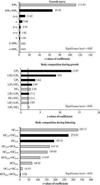
Response surface analysis for LIPGobs output was performed for Charolais cows characterized by the standard input values (Table 5). Various modules of the model were considered: the growth curve (Eqn 4, Table 2), body composition during growth and body composition during finishing. Taking into account the results in Table 5, response surface analysis was not conducted for the parameters of the body gain curve during finishing. Figure 3 shows the levels of significance for each parameter estimate of the response surface fitting curve for the three modules. Consistent with the NSCs, the growth curve module exhibits significance for BW0 and its quadratic term with positive effect of BW0 on the gain in lipid, but negative effect of the quadratic term. Parameter a and the quadratic term for parameter b were also significant. For the module of body composition during growth, the effects of the parameters LIP0, LIPa and DC0 and their cross and quadratic terms were investigated. DCa was not taken into account because of its low impact, similar to the low impact of DC0. All the terms in the equation were significant, except the interaction between LIPa and DC0. The highest t-value coefficients were obtained for LIP0 and its quadratic term as shown in Fig. 3.
The t-values of the coefficients obtained from the response surface analysis of LIPGobs against the parameters of CompoCow related to growth curve, body composition during growth and body composition during finishing. The Significance level of 0·05 is indicated by the dashed line. Bars are black when the effect of the factor on LIPGobs is positive and grey when it is negative.

For the module on body composition during finishing, the analysis was performed with the parameters DCend, DClean and BCSlean. Figure 3 shows that the main effects were obtained with parameters DCend and DClean, which is consistent with Table 5. Their interaction also has a significant effect on the level of lipid gain.
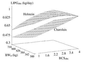
Figure 4 shows the shapes of the response surfaces of LIPGobs to the BCS of the observed animal, and to the BW0 parameter for Charolais and Holstein cows characterized by their standard input values (Table 4, except for BCSobs). The values of LIPGobs vary from 0·45 (for a very lean cow and highest value of BW0), to 0·85 (for a very fat cow and lowest BW0) in Charolais cows, whereas LIPGobs varies from 0·60 to 0·94 in Holstein cows. The curves obtained show that the model predicts higher lipid gain in Holstein than in Charolais cows, at the same empty BWG. However, the shapes of the curves are not strictly parallel because the response is linear for Charolais cows, whereas the response is quadratic for Holstein cows. Surface response for Holstein cows exhibits a plateau because the LIPGobs achieves its maximum, which occurs when empty BWG only contains lipid.
Response surface for the output variable LIPGobs, i.e. the level of lipid in gain, to the input values for BCSobs and BW0, for the Charolais and Holstein cow calibration.

Model testing
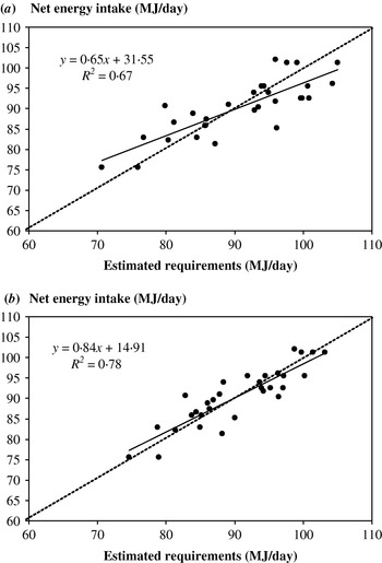
Figure 5 shows the level of NE intake per day for the 31 groups of Charolais cows during finishing, depending on the NE requirements estimated with the previous recommendations (Fig. 5a) and estimated with CompoCow (Fig. 5b). The accuracy and precision of the estimates are better with CompoCow than with the previous recommendations. Indeed, the shape of the regression of observed v. predicted shows a lower rotation and higher correlation. The regression slope was closer to 1 (0·84 and P=0·055 v. 0·65 and P<0·0005) and the intercept was closer to 0 (1·96 v. 4·1). Mean bias obtained with CompoCow was lower (−0·01 v. 0·06) and the coefficient of determination was higher (R 2=0·78 v. R 2=0·67). Moreover, the residual mean squared deviation was lower with CompoCow (0·46) than with previous recommendations (0·67). Investigation of the residuals did not highlight any significant tendency with CompoCow, whereas the previous recommendations tended to overestimate the energy requirements for the groups with BWGobs higher than 1·2 kg/day and to underestimate the requirements for the groups with an average age of more than 7 years.
Graphs of the observed NE intake of the 31 groups of Charolais cows at finishing against the requirements estimated (a) using previous recommendations (INRA Reference Jarrige1989) and (b) with the CompoCow model.

DISCUSSION
The CompoCow model was built to estimate more precisely and accurately the energy requirements of culled cows during finishing under a wide range of practical situations. CompoCow should be able to estimate correctly the evolutions of cow body composition during finishing, taking into account the factors involved: BW, BCS, frame size and age. CompoCow does not detail the different parts of the animal, i.e. carcass and viscera, whereas it is known that these compartments evolve differently (Jenkins & Ferrel Reference Jenkins and Ferrel1997). CompoCow does not account either for different efficiencies for energy intake utilization, for maintenance, to support metabolism, and for energy retained in gain, as in the model of Williams & Jenkins (Reference Williams and Jenkins2003a, Reference Williams and Jenkinsb). For the purpose of recommendation, it was considered that the best model should give robust predictions with the least number of parameters to estimate. The capacities of the model were investigated to simulate the qualitative evolutions of composition of body gain and predict the energy requirements of culled cows during finishing.
Model response to key determinants of lipid proportion in the gain
The main characteristic of the composition of gain during finishing (for culled cows and other bovine animals) is that the proportion of lipid in body mass gain increases during the finishing period (Wright & Russel Reference Wright and Russel1984). Indeed, proportions from 0·28 to 0·90 of lipid in gain have been reported (Wright & Russel Reference Wright and Russel1984; Agabriel & Petit Reference Agabriel and Petit1987; Robelin et al. Reference Robelin, Agabriel, Malterre and Bonnemaire1990; Jenkins & Ferrel Reference Jenkins and Ferrel1997; Fiems et al. Reference Fiems, Van Caelenbergh, Vanacker, De Campeneere and Seynaeve2005) for culled cows according to conditions and genotypes. For example, Fiems et al. (Reference Fiems, Van Caelenbergh, Vanacker, De Campeneere and Seynaeve2005) found a proportion of 0·35 of lipid in body mass gain for Belgian Blue cows increasing their BW by 188 kg during finishing. Robelin et al. (Reference Robelin, Agabriel, Malterre and Bonnemaire1990) found a proportion of 0·78 of lipid in a 114 kg body mass gain for Holstein cows. From the point of view of model behaviour, BW and BCS increase during finishing. The current sensitivity analysis showed that CompoCow predicts that the proportion of lipid increases with increasing BWobs and BCSobs (Table 4), which means that it calculates increasing proportions of lipid in gain over the finishing period. This result shows that the model's behaviour is qualitatively consistent with experimental observations from the literature. Moreover, the values calculated with a BWG of 1 kg/day range from 0·45 to 0·85 in Charolais cows and from 0·60 to 0·94 in Holstein cows, which is also quantitatively consistent with the results of Agabriel & Petit (Reference Agabriel and Petit1987) and Robelin et al. (Reference Robelin, Agabriel, Malterre and Bonnemaire1990). The model's construction also allows for simulating different proportions of lipid to account for early and late maturing breeds. Consistently, increase in BWobs and BCSobs results in increasing energy for gain and increasing energy requirements. This is in accordance with the statement of Cabaraux et al. (Reference Cabaraux, Dufrasne, Roux, Istasse and Hornick2005) that a cow culled at high condition score will gain weight as if it had already begun its finishing period and will have a lower feeding efficiency than a cow culled at a lean condition score.
Malterre (Reference Malterre and Micol1986) reported that age of the cow has a negative effect on its ability to gain weight and to fatten. Cabaraux et al. (Reference Cabaraux, Dufrasne, Roux, Istasse and Hornick2005) linked this effect to the increase in the initial BW during finishing with age, which induces higher maintenance requirements and a lower feeding efficiency. These authors also mentioned an increase in the proportion of lipid in body gain during finishing with age. It is noteworthy that the experiments mentioned by Malterre (Reference Malterre and Micol1986) show that BWG during finishing significantly decreases for Salers cows up to 8 years old, Normandy cows up to 10 years old and Holstein cows up to 6 years old. These thresholds correspond mainly to old ages relative to the actual average age of culling. Unexpectedly, the effect of the age of the cow on the proportion of lipid in gain with CompoCow was practically nil as shown by the NSCs. These coefficients were calculated with the attributes of the reference cow having the same age, to avoid misunderstanding due to interactions between inputs. However, as mentioned by Cabaraux et al. (Reference Cabaraux, Dufrasne, Roux, Istasse and Hornick2005) and Malterre (Reference Malterre and Micol1986), the increase in age results in higher BW of the animal (with a similar BCS) and the model predicts an increase in the proportion of lipid in gain and in the requirements with BW. In this sense, the model remains consistent with experimental observations.
Prediction of energy requirements during finishing
Sensitivity analysis and model testing provided information about the model's behaviour, about the parameters that are important for predictions and about its predictive ability. It was identified that the model (i) is mainly sensitive to inputs, and to parameters BW0, DClean and DCend, and (ii) predicts accurately and quite precisely the energy requirements of culled Charolais cows during finishing.
Sensitivity of CompoCow to the inputs BWobs, BCSobs and frame size is very important and stresses the need for their accurate estimation for on-farm prediction. They are the key determinants of the energy requirements in the model. The results in Table 5 showed that the model is also highly sensitive to BW0, DClean and DCend, which means that accurate and precise estimates of these parameters are required to use the model. BW0 corresponds to BW at 3 years old, and is the initial value of the fitted Gompertz curve. This parameter is very important in estimating BWref and the position of observed BW relative to BWref determines where the animal is theoretically positioned on the finishing curve. Through this parameter BW0, it is the reference BW and its associated body condition that are of importance. Several authors have developed models that rely on reference BWs at maturity, or reference BW curves (Sanders & Cartwright Reference Sanders and Cartwright1979a, Reference Sanders and Cartwrightb; Bruce et al. Reference Bruce, Broadbent and Topps1984; Williams & Jenkins Reference Williams and Jenkins1997, Reference Williams and Jenkins2003a, Reference Williams and Jenkinsb). This reference at maturity is usually defined by BW and proportion of adipose tissue, which is usually 0·25 (Sanders & Cartwright Reference Sanders and Cartwright1979a, Reference Sanders and Cartwrightb; Williams & Jenkins Reference Williams and Jenkins1997). However, in this case, a reference BW at maturity is defined, associated with a proportion of lipid, but also a reference BW, associated with a proportion of lipid at each age and for each frame size.
Sensitivity of the model to parameters DClean and DCend is linked to the impact of these parameters on empty BWG, at a constant body weight gain. Indeed, an increase of DClean and/or a decrease of DCend result in an increase in empty BWG, and in lipid gain, whereas the proportion of lipid in gain slightly decreases.
Testing of CompoCow with the Charolais dataset showed that the model predicts accurately and precisely the energy requirements during finishing of groups of cows. It performs better than the previous recommendations based on experimental observations (INRA Reference Jarrige1989). Interestingly, CompoCow did not induce any bias according to the age of the animals, whereas (i) the model exhibited low sensitivity to the observed age and (ii) the previous recommendations underestimated the requirements for culled old cows. This result confirms that the scheme that links a growth model to a finishing model is of interest. It highlights the fact that there are great interactions between age and other animal characteristics, and that CompoCow is able to predict the requirements of cows of various ages.
Model testing was performed with an adjustment in the λ coefficient for estimating maintenance requirements. It appears that adjusted maintenance requirement is higher than current values for adult dry cows. This result is, however, consistent with the hypothesis of Williams & Jenkins (Reference Williams and Jenkins2003a) that links maintenance energy to the level of feeding. Indeed, maintenance requirements are of great importance for estimating energy requirements and difficult to estimate experimentally in many situations. Results from the literature show that maintenance requirements are linked to metabolic weight but also to viscera weight (Chilliard et al. Reference Chilliard, Doreau, Bocquier, Lobley, Journet, Grenet, Farce, Theriez and Demarquilly1995). Moreover, observations do not give a clear insight into the effect of condition score on maintenance requirements (Houghton et al. Reference Houghton, Lemenager, Hendrix, Moss and Stewart1990; Ortigues et al. Reference Ortigues, Petit and Agabriel1993; Birnie et al. Reference Birnie, Agnew and Gordon2000). Consequently, this mathematical formulation is a major simplification of the biological process, and further testing of the model will evaluate the error that is made with this simplification. Complete validation of CompoCow will only be achieved when there is more varied experimental data to test and adjust the model for several beef and dairy breeds.
CONCLUSION
CompoCow is a predictive model of body composition, gain composition and energy requirements for culled cows during finishing. CompoCow is quite simple to use for the purpose of recommendations but our results show that it is robust. This model is now available in the INRA system for determining culled cow requirements and it will be available in INRAtion software (v4.0). Further work will include model calibration and testing with new datasets, involving several beef and dairy breeds to achieve model validation without fitting the maintenance coefficient.
The main novel feature of CompoCow lies in its association of two BW curves working at two different time scales: one curve for growth during lifetime performance and one curve for gain during finishing. The approach adopted would also be relevant for predicting the requirements of cows during their lifetime performance. In this case, the model would associate a growth curve dependent on age (in years) and one or several equations for weight variations around the growth curve. These equations would express how the animal draws on its own resources of lipid at the beginning of lactation and how it stores lipid during late lactation.
The authors are very grateful to the staff of the experimental farms Laqueuille, Marcenat, Les Cèdres and Orcival, and to the staff of the Theix slaughterhouse for data provision. We also thank J. Curtis Williams and an anonymous referee for English revision of the manuscript.