1. Introduction

Bayesian inference is a well-established theory of uncertain reasoning that represents agents’ epistemic attitudes—their degrees of belief—by the laws of probability (e.g., Jeffrey Reference Jeffrey1965; de Finetti Reference de Finetti1972; Savage Reference Savage1972; Earman Reference Earman1992; Bovens and Hartmann Reference Bovens and Hartmann2003). A probability function p(H) represents a rational agent’s degree of belief that H is true. On learning evidence E, the agent adopts a posterior belief in H according to the rule of conditionalization: $p^E\left(H\right)=p\left(H\right|E)$ . Such posterior degrees of belief serve as a basis for assessing hypotheses and making decisions—also in the context of public policy. For example, the assessment reports of the International Panel for Climatic Change evaluate the probability of future events as experts’ subjective degrees of belief.

Why are these posterior degrees of belief something else than arbitrary subjective attitudes? Why can they guide rational and efficient decisions? Presumably it is because they are in some way informed by objective evidence. Indeed, if we look at Bayes’s theorem,

$\begin{array}{cc}p\left(H\right|E)& =p\left(H\right)\frac{p\left(E\right|H)}{p\left(E\right)}\\ & ={\left(1+\frac{1-p\left(H\right)}{p\left(H\right)}\cdot \frac{p\left(E\right|\neg H)}{p\left(E\right|H)}\right)}^{\mathrm{-1}},\end{array}$

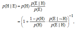
we see that an agent’s posterior degree of belief in H depends on three factors: her prior degree of belief in H, p(H), and the conditional degrees of belief $p\left(E|H\right)$ and $p\left(E\right|\neg H)$ —often called the likelihoods of H and ¬H on E. Bayesians contend that as long as the prior degrees of belief in H are not too extreme, a “well-designed experiment … will swamp divergent prior distributions with the clarity and sharpness of its results, and thereby render insignificant the diversity of prior opinion” (Suppes Reference Suppes, Hintikka and Suppes1966, 204). Clearly, any such merging-of-opinion argument makes the tacit assumption that $p\left(E|H\right)$ and $p\left(E\right|\neg H)$ are objectively constrained.

The reliance of Bayesians on such constraints is even more explicit in the Bayes factor—a standard measure for summarizing experimental observations and quantifying the weight of evidence in favor of a hypothesis (Jeffreys Reference Jeffreys1961; Kass and Raftery Reference Kass and Raftery1995). It is defined as the ratio of prior and posterior odds between two competing hypotheses H₀ and H₁:

${\mathrm{BF}}_{10}\left(E\right)=\frac{p\left(H_1\right|E)/p(H_0\left|E\right)}{p\left(H_1\right)/p\left(H_0\right)}\mathrm{.}$

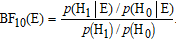
It follows from Bayes’s theorem that the Bayes factor is a ratio of two conditional degrees of belief: ${\mathrm{BF}}_{10}\left(E\right)=p\left(E\right|H_1)/p(E\left|H_0\right)$ . Thus, the Bayes factor is only as objective and nonarbitrary as $p\left(E\right|H_0)$ and $p\left(E\right|H_1)$ are.Footnote ¹

The idea that such conditional degrees of belief are rationally constrained and temper the influence of subjectively chosen priors stands at the basis of many attempts to defend the rationality and objectivity of Bayesian inference (e.g., Earman Reference Earman1992, chap. 6). It is usually taken for granted that they are aligned with objective probabilities derived from the relevant statistical model. For example, if H denotes the hypothesis that a die is fair and E the outcome of two sixes in two tosses, then it appears rational to have the conditional degree of belief $p\left(E|H\right)=1/36$ . However, none of the familiar stories for justifying this alignment (e.g., reliance on chance-credence coordination principles) is convincing as it stands.

Pointing out this justification gap is the main task of the negative part of the article. In particular, I argue that neither the ratio analysis of conditional probability nor chance-credence coordination principles explain why conditional degrees of belief are rationally constrained by the corresponding objective probabilities (sec. 2). The constructive part of the article solves the problem in a Ramsey–de Finetti spirit: $p\left(E|H\right)$ is the degree of belief in the occurrence of E upon supposing that the target system’s behavior is described by H. I work out the details of this suppositional analysis in the context of statistical inference: the relevant set of possible worlds for evaluating conditional degrees of belief, their alignment with density functions of statistical models, and how chance-credence coordination guides Bayesian inference and supports claims to objectivity (sec. 3).

In the final part of the article, I explore the general implications of my approach, focusing on a pertinent problem of Bayesian inference: the interpretation of highly idealized statistical models in which important causal factors are omitted or functional dependencies are simplified. Such models are used in disciplines as diverse as psychology, economics, and climate science. In such cases, it would be inappropriate to interpret the probability of a model as the degree of belief in its (approximate) truth. Nonetheless, as Bayesian reasoners, we rank different idealized models according to their posterior probability, and we use these rankings in inference and decision making. So we need to explain what these probabilities mean, if not degrees of belief in the truth of the model.

I argue that the problem vanishes when all probabilities in Bayesian inference, including prior and posterior degrees of belief, are understood as conditional degrees of belief relative to an overarching model. Then I explain how this extension of the suppositional analysis squares with various principles for determining rational prior degrees of belief, including a recent proposal by Olav Vassend (sec. 4). Moreover I show how we can use Bayesian models for prediction, theory evaluation, and decision making, even when models are highly idealized and not faithful to reality (sec. 5). Finally I wrap up the results of the article (sec. 6).

The suppositional approach is not novel. Ramsey (Reference Ramsey and Mellor1929/1990) famously argued that a conditional degree of belief in a proposition E given another proposition H is determined by supposing H and reasoning on that basis about E. However, my article is, to the best of my knowledge, the first one to explicate the mechanics of the suppositional approach in the context of statistical inference, to make precise the role of chance-credence coordination in this process, and to explain why such conditional degrees of belief are universally shared.Footnote ² It is also the first exploration of the implications of the suppositional approach for contexts in which no model is a serious contender for (approximative) truth and for practical decisions based on statistical models. Thus, it provides the conceptual groundwork for numerous applications of Bayesian inference in statistics and other domains of science.

2. “The Equality” and Probability in Statistical Models

What constrains the conditional degree of belief in an observation E, given a statistical hypothesis H? A classical illustration is an inference about the bias of a coin. The hypotheses (H_μ, $\mu \in (0,1)$ ) describe how likely it is that the coin will come up heads on any individual toss. When the tosses are independent and identically distributed (i.i.d.), we can describe the outcome of N repeated coin tosses by the observation E_k (=k heads and $N-k$ tails), whose probability follows the binomial probability density function 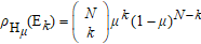${\rho }_{H_{\mu }}\left(E_k\right)=\left(\begin{array}{c}N\\ k\end{array}\right){\mu }^k{(1-\mu )}^{N-k}$ .Footnote ³

Suppose that we consider the hypothesis that a coin is slightly biased toward tails: it comes up heads only 40% of the time ($H_0:\mu =.4$ ). This implies that the probability of observing two heads in two i.i.d. tosses (=E) is equal to 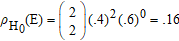${\rho }_{H_0}\left(E\right)=\left(\begin{array}{c}2\\ 2\end{array}\right){\left(.4\right)}^2{\left(.6\right)}^0=.16$ . Bayesian reasoners align their conditional degrees of belief $\rho \left(E\right|H_0)$ with the relevant value of the probability density function ${\rho }_{H_0}$ , that is, ${\rho }_{H_0}\left(E\right)$ (e.g., Bernardo and Smith Reference Bernardo and Smith1994; Howson and Urbach Reference Howson and Urbach2006). And since the latter is uniquely determined, so is the former. Having “objective” conditional degrees of belief $p\left(E\right|H_0)$ leads to (approximate) long-run consensus on posterior distributions and unanimous assessments of the strength of observed evidence, for example, via the Bayes factor. For the above evidence E and the two competing hypotheses $H_0:\mu =.4$ and $H_1:\mu =.8$ , all of us will presumably adopt the conditional degrees of belief $p\left(E\right|H_0)=.4\times .4=.16$ and $p\left(E\right|H_1)=.9\times .9=.81$ and report a Bayes factor ${\mathrm{BF}}_{10}\left(E\right)=.81/.16\approx 5.06$ , corresponding to moderate evidence for H₁. This evidential judgment is supposed to be shared by all Bayesian reasoners, regardless of their priors over H₀ and H₁. It rests, however, on an alignment between density functions of a statistical model and conditional degrees of belief that is not easy to justify.

In other words, we require a satisfactory answer to the following question:

A traditional approach to conditional degrees of belief, proposed by various textbooks on Bayesian inference (e.g., Jackson Reference Jackson1991; Earman Reference Earman1992; Skyrms Reference Skyrms2000; Howson and Urbach Reference Howson and Urbach2006), evaluates them as the ratio of two unconditional probabilities: $p\left(E|H\right)=p(E\wedge H)/p\left(H\right)$ whenever $p\left(H\right)>0$ . While this ratio analysis (Hájek Reference Hájek2003) is uncontroversial as a mathematical constraint on conditional probability, it does not explain the equality. First, if ρ_H(E) determines $p\left(E|H\right)$ , it must do so directly and not be mediated by unconditional degrees of belief. The counterparts of $p(E\wedge H)$ and p(H) are undefined within the statistical model (e.g., the binomial distribution). Second, ratio analysis neglects a robust empirical fact: we usually evaluate conditional degrees of belief $p\left(E|H\right)$ directly, rather than by reasoning about $p(E\wedge H)$ and p(H) and calculating their ratio (see also Hájek [Reference Hájek2003] and the experiments in Zhao, Shah, and Osherson [Reference Zhao, Shah and Osherson2009]). Third and last, ratio analysis is silent whenever $p\left(H\right)=0$ , but such hypotheses are omnipresent in statistical inference with real-valued parameters. For example, a uniform prior distribution—in fact, any continuous distribution—over the parameter μ in the binomial model implies that any precise hypothesis such as $H:\mu =.4$ has probability zero.

A frequently used alternative strategy for justifying the equality consists in invoking a chance-credence coordination principle: subjective credences should follow known objective chances. The most famous of these is the Principal Principle (PP; Lewis Reference Lewis and Jeffrey1980): the initial credence function of a rational agent, conditional on the proposition that the physical chance of E takes value x, should be equal to x. A similar intuition with an eye on applications to statistical inference is expressed by the Principle of Direct Inference (PDI; e.g., Reichenbach Reference Reichenbach1949; Kyburg Reference Kyburg1974; Levi Reference Levi1977, Reference Levi1980): for instance, if I know that a die is unbiased, I should assign degree of belief 1/6 that any particular number will come up.

Transferring these principles to the equality is, however, not as straightforward as it looks. True, the value ρ_H(E) does not depend on subjective credences but on the objective properties of a given statistical model. This seems to be a sufficient reason for classifying ρ_H(E) as an objective chance, and then PP or PDI determines the value of the conditional degree of belief $p\left(E|H\right)$ (see also Earman Reference Earman1992, 54–56).

This strategy neglects that chance-credence coordination principles understand objective chances as making empirical statements: their values depend on “facts entailed by the overall pattern of events and processes in the actual world” (Hoefer Reference Hoefer2007, 549). Dependent on the preferred conception of objective chance, such facts could be the setup of a statistical experiment or the composition and precise shape of a die that we roll. However, the truth conditions of sentences such as ${\rho }_H\left(E\right)=1/36$ are entirely internal to the statistical model. Suppose that H denotes the hypothesis that a die in front of us is unbiased, and E denotes the observation of two sixes in two i.i.d. rolls. Then the sentence

has no empirical content—it may even strike us as analytically true. Note that Dice Roll does not refer to real-world properties or events: even if no perfectly unbiased dice existed in the actual world (and perhaps this is actually the case), the sentence would still be true. The probability ρ_H(E) is objective in the sense of being subject independent but is not a physical chance in the sense of being realized in the actual world (Rosenthal Reference Rosenthal2004; Sprenger Reference Sprenger2010). This diagnosis is typical of probability in statistical models.

For this reason, neither the PP nor the PDI solves our problem. The principles coordinate our degrees of belief with known chancy properties of the actual world. But the objective probabilities in question, ρ_H(E), do not express physically realized chances. Therefore, standard chance-credence coordination principles cannot directly justify the equality. A more sophisticated story has to be told.

3. The Suppositional Analysis

This section develops and defends a suppositional analysis of conditional degree of belief: conditional degrees of belief constitute a primitive epistemic concept and we determine our degree of belief in E given H by supposing that H is true. Two famous Bayesians—the British philosopher Frank P. Ramsey and the Italian statistician Bruno de Finetti (Reference de Finetti1972, Reference de Finetti2008)—have proposed this view in the literature. I focus on Ramsey since de Finetti also requires that H be a verifiable event if $p\left(E|H\right)$ is to be meaningful (de Finetti Reference de Finetti1972, 193). This verificationism is unnecessarily restrictive for our purposes.

Here is Ramsey’s famous analysis of conditional degrees of belief: “If two people are arguing ‘if H will E?’ and both are in doubt as to H, they are adding H hypothetically to their stock of knowledge and arguing on that basis about E. We can say that they are fixing their degrees of belief in E given H” (Reference Ramsey and Mellor1929/1990, 155, my emphasis). Put differently, we evaluate the conditional degree of belief $p\left(E|H\right)$ by supposing the truth of the conditioning proposition H and by assessing the plausibility of E given this supposition. Ramsey’s analysis has also inspired various accounts of evaluating (the probability of) indicative conditionals (e.g., Stalnaker Reference Stalnaker and Rescher1968; Adams Reference Adams1975; Levi Reference Levi1996), but these questions go beyond the scope of this article.

While we have an intuitive grasp of how Ramsey’s proposal is supposed to work, we need a more detailed account of its mechanics to explain why statistical reasoners typically agree on the relevant conditional degrees of belief. Consider a target system S (e.g., repeated dice rolls) described by a statistical hypothesis H (e.g., “the die is fair”). Supposing H defines a possible world ω_H, or more precisely a set of possible worlds, where the behavior of S is governed by ρ_H. Given that these possible worlds may differ from one another in features that are unrelated to S, which one is relevant for fixing our degrees of belief? Do we need to choose the closest possible world—a notoriously vague and difficult concept (Lewis Reference Lewis1973a)—to settle the matter?

Fortunately, choosing is not necessary. Let $\left[{\omega }_{H,S}\right]\subset 𝒲$ denote the set of worlds where the behavior of S is governed by the probability law H. Supposing H is best explicated as restricting the space of relevant possible worlds to [ω_H,S]. In particular, in any such world, the objective chance of an observation E is given by ρ_H(E).Footnote ⁴

The differences between the elements of [ω_H,S] are not relevant for our purposes. Typically, the scope of a statistical model does not go beyond the target system it aims to model. For example, in an experiment in which we roll a die, the hypotheses correspond to (multinomial) distributions describing the die’s specific properties. Similarly, the possible outcomes E, E′, E″, and so on (e.g., three sixes in a row), are contained in our statistical model of S. In any possible world that belongs to [ω_H,S], the outcome E will therefore have the same probability. This invariance is a notable difference between applying the suppositional analysis in the context of statistical inference and to conditional degrees of belief more generally.

Supposing H may be in conflict with available background knowledge about the target system. For this reason, my interpretation of conditional degrees of belief differs from Ramsey’s in a crucial nuance: where Ramsey suggested that H is added to existing background knowledge, on my account H may also overrule conflicting information. In such cases, we obtain a genuinely counterfactual interpretation of conditional degrees of belief. This is often necessary: we may know that a given die is biased, that the rolls are not i.i.d., and so on. But for my analysis, it does not matter whether assuming H is consistent or in conflict with our background knowledge: the above recipe for constructing the set [ω_H,S] applies in either case.

The dice-rolling example shows how the suppositional analysis ensures alignment of conditional degrees of belief with probability densities. Let H denote the hypothesis that the die on the table is fair. Consider a world ${\omega }_H\in \left[{\omega }_{H,S}\right]$ . As explained above, supposing H implies that within ω_H, the objective, physical chance of rolling (at least) one six in one toss is 1/6, in two (i.i.d.) tosses it is 11/36, and so on. Since ω_H is by definition a chancy world, these chances should inform our degrees of belief via the PDI or the PP. After all, ρ_H describes the physical chances that hold for S in ω_H, and we have no reason to challenge the rationality of PDI or PP in this case.Footnote ⁵ Thus, for any event E in target system S, our (unconditional) degrees of belief within ω_H should satisfy $p_{{\omega }_H}\left(E\right)={\rho }_H\left(E\right)$ . By definition of the suppositional analysis of conditional degrees of belief, we also have 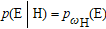$p\left(E\right|H)=p_{{\omega }_H}\left(E\right)$ . 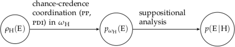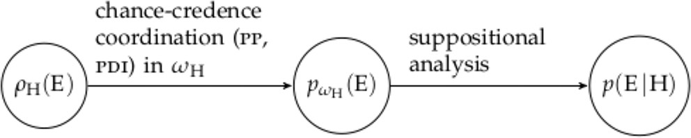Combining both equations yields $p\left(E\right|H)={\rho }_H\left(E\right)$ : conditional degrees of belief track probability density functions (see also fig. 1).Footnote ⁶ Taken together with uncontroversial principles for chance-credence coordination, the suppositional analysis of conditional degrees of belief establishes the equality and explains the seemingly analytic character of sentences such as Dice Roll. In particular, there is no room for rational disagreement on such conditional degrees of belief.

Figure 1.

Two steps in justifying the equality: chance-credence coordination transfers the probability density ρ_H(E) to the rational ω_H degree of belief in E, $p_{{\omega }_H}\left(E\right)$ , and the suppositional analysis connects that value to $p\left(E|H\right)$ .

This agreement transfers to statistical measures of evidence that are derived from these conditional degrees of belief and play a pivotal role in statistical inference, such as Bayes factors. Hence, we can explain where the objective elements in Bayesian inference come from: probability density functions determine conditional degrees of belief (i.e., the likelihoods) and constrain measures of evidence such as Bayes factors. Via Bayes’s theorem, they also constrain posterior probabilities (see sec. 5 for more details).

It is important to understand the role of the PDI and the PP in the suppositional analysis. Standardly, both principles apply to real-world, ontic chances, for example, “the chance of this atom decaying in the next hour is 1/3” or “the chance of a zero in the spin of this roulette wheel is 1/37.” The principles claim that degrees of belief should mirror physical chances whenever we know them. Compare this to the picture that we sketch for conditional degrees of belief: we do not deal with real-world chances; rather we observe that in the worlds in the set [ω_H,S], the physical chance of E is given by ρ_H(E). In other words, we do not apply PDI or PP in the actual world ω_@ but in a counterfactual world ω_H described by H. By supposing that the occurrence of E is genuinely chancy and follows the probability law ρ_H(E), the suppositional analysis gives a role to chance-credence coordination principles in statistical inference, explaining why our conditional degree of belief in E given H is uniquely determined and obeys the equality. Note that our application of PDI or PP pertains to unconditional degrees of belief (i.e., $p_{{\omega }_H}\left(E\right)$ ) and is therefore fully analogous to those physical-chance examples that motivate the principles in the first place.

Transferring chance-credence coordination from actual to counterfactual worlds is a distinct strength of the proposed account, and a crucial difference to competing accounts that introduce a distinct chance predicate, and chance propositions in our corpus of background knowledge (Levi Reference Levi1980, 254–56). So much the more as the existence of physical chances in the real world is a contested issue, especially outside some foundational areas of science such as quantum physics. If chance-credence coordination in the actual world were supposed to justify the equality, the Bayesian would need an argument that physical chances actually exist for the system she is studying and that they are expressed by the values of ρ_H. Such a claim would be hard to prove and make strong ontological commitments. Instead, the probabilities given by the model’s density functions ρ_H should be understood as physical chances in hypothetical scenarios. Chance-credence coordination should apply upon the supposition of such a hypothetical scenario and not in the actual world.

This agnostic attitude to physical chance matches the practice of non-Bayesian statistical inference, too. Here are the thoughts of the great frequentist statistician Ronald A. Fisher on conditional probability in hypothesis testing: “In general tests of significance are based on hypothetical probabilities calculated from their null hypotheses. They do not lead to any probability statements about the real world” (Reference Fisher1956, 44). That is, Fisher is emphatic that the conditional probability of data given some hypothesis has a hypothetical character and is not a physically realized objective chance. Probabilities are useful instruments of inference, not components of the actual world. According to Fisher, probabilistic reasoning and hypothesis testing is essentially counterfactual: it is based on the probability of observations under an idealized and most likely false hypothesis that we suppose for the sake of the argument.

Before proceeding, I recap the essential elements of the proposed suppositional analysis. The starting point is Ramsey: the conditional degree of belief in observation E given statistical hypothesis H is equal to the belief in E that we have upon supposing that H is the true model of target system S. This hypothetical scenario corresponds to a set of possible worlds [ω_H,S] where S follows the probabilistic law defined by H. In this stochastic world [ω_H,S], we apply standard chance-credence coordination principles and calibrate our degree of belief in E with the known objective chance of E, given by the density function ρ_H(E). Thus, we obtain the equality. The suppositional approach to conditional degree of belief also relieves us of the worry to make sense of $p\left(E|H\right)$ in the frequently occurring cases in which $p\left(H\right)=0$ . In these cases, probabilities of the type $p\left(E|H\right)$ fall outside the scope of (standard) ratio analysis, but for us, they have determinate values since the suppositional analysis is feasible regardless of the probability of H. I will now explore the implications of the suppositional analysis for Bayesian inference in general.

4. Implications: Model-Relative Prior Probabilities

The suppositional analysis has focused on the relationship between statistical hypothesis H and observation E and said little about the background assumptions in the statistical model ℳ. Consider again the case of tossing a coin, assuming that the tosses are i.i.d. This assumption is not expressed in a hypothesis such as “the coin is fair” or “the coin is slightly biased toward tails.” Differences between the competing hypotheses are typically expressed by means of different parameter values, such as $H:\mu =1/2$ versus $H^{\prime }:\mu =.4$ , $H^{″}:\mu =.9$ , and so on. The statement of the hypothesis does not comprise essential assumptions about the experimental setup such as independence and identical distribution of the coin tosses.

Introducing the notion of a statistical model $ℳ=(𝒮;𝒫)$ (Cox and Hinkley Reference Cox and Hinkley1974; McCullagh Reference McCullagh2002) helps to clarify matters. It consists of two parts: the sample space 𝒮 and the set of probability distributions 𝒫 over 𝒮, such as the binomial distributions B(N, μ) that describe the repeated toss of a coin. All these distributions presuppose the sample size N and that the individual tosses are i.i.d. Therefore, the hypotheses in ℳ only differ regarding the value of μ, and for purposes of comparisons we can write them as $H:\mu =1/2$ , $H^{\prime }:\mu =.4$ , and so on.

Note that real coin tosses are often far from being i.i.d. Nevertheless, restriction to the family of binomial distributions can be a useful and efficient way to study the bias of the coin. We do, in practice, almost never consider the “catchall” hypothesis that our model is wrong. Instead, we just ask what we can learn about target system S given a certain degree of idealization and abstraction.

This observation connects to a classical problem of Bayesian inference mentioned in the introduction (see also Walker Reference Walker2013; Wenmackers and Romeijn Reference Wenmackers and Romeijn2016; Vassend Reference Vassend2019). Bayesians interpret p(H) standardly as the prior degree of belief that the hypothesis H is true. However, H may be part of a highly idealized statistical model of the target system that simplifies functional dependencies or neglects causally relevant factors (e.g., because the effect size is too small to be relevant). Such idealized models occur in all fields of science and are particularly common in disciplines in which causal relationships are messy and hard to isolate, such as psychology, economics, and climate science.

In such cases, it is highly unlikely that our hypothesis H is literally true, that it sketches a faithful picture of reality. Regardless of how probable H is with respect to other hypotheses in the overarching model ℳ (e.g., H′, H″), we would not be prepared to enter any bet on the truth of H. But if this is the case, how can we entertain a strictly positive degree of belief in H? In other words, why do we assign a positive degree of belief p(H) in our Bayesian model and not probability zero?Footnote ⁷

In other words, we face the trilemma of having to reject one of the following three jointly inconsistent propositions (Sprenger and Hartmann Reference Sprenger and Hartmann2019, chap. 12):

1. 1. The expression $p\left(H\right)>0$ denotes a Bayesian agent’s degree of belief that H is true.

2. 2. The hypothesis H is part of a general statistical model ℳ with a partition of hypotheses $\mathscr{H}=\left\{H,H^{\prime },H^{″},\dots \right\}$ .

3. 3. The model ℳ is a strong idealization of reality and likely or known to be false.

The second and third propositions are commonly acknowledged facts about statistical modeling and cannot be rejected as long as we aim at a rational reconstruction of Bayesian inference in science. So we have to give up the first proposition and to rethink the interpretation of prior probabilities in Bayesian inference. When the underlying models are sufficiently idealized, they cannot denote an agent’s honest degrees of belief that a hypothesis is true.

Note that the introduction of a “catchall hypothesis” $\tilde{H}=\neg \left(H\vee H^{\prime }\vee H^{″}\vee \dots \right)$ into ℳ (e.g., Earman Reference Earman1992) does not solve the problem. Since the model ℳ is highly idealized, we would have to concentrate all probability mass on $\tilde{H}$ . This means that we could not differentiate among H, H′, H″, and the other hypotheses in ℳ: their prior and posterior probability would always be zero or arbitrarily close to that value.

Extending the suppositional analysis solves the problem: if ℳ describes the overarching statistical model and H is one of the hypotheses in ℳ, then all probability assignments are relative to ℳ. The degree of belief in the truth of H that we would have if we had supposed that the target system is fully and correctly described by one of the hypotheses in ℳ is expressed by p _ℳ(H). In fact, Bayesian modelers distribute prior degrees of belief only over elements of 𝒫. This perspective on prior probabilities, which flows logically from our take on conditional degrees of belief, resolves the above trilemma: we deny premise 1 that p(H) denotes an actual degree of belief. Any such probability is, like the probabilities of evidence given a hypothesis, essentially hypothetical and should be read as p _ℳ(H). Similarly, $p\left(E|H\right)$ should always be read and understood as the model-relative conditional degree of belief $p_{ℳ}\left(E|H\right)$ .

Suppositional or hypothetical prior probabilities are, however, not rationally constrained in the same way as $p_{ℳ}\left(E|H\right)$ . In particular, supposing ℳ need not define any objective chances in ω_ℳ,𝒮. Thus, unlike in the case of $p_{ℳ}\left(E|H\right)$ , the suppositional analysis does not yield a uniquely rational degree of belief for p _ℳ(H) or offer any guidance “how we are supposed to understand and evaluate counterfactual probabilities,” as Vassend (Reference Vassend2019, 711) writes in a congenial contribution.

Vassend makes his observation in a critical spirit, but I would like to embrace it. Subjective Bayesian inference allows for different rational choices of the prior distribution upon supposing a model ℳ and remains silent on which factors determine this choice. If p _ℳ(H) were determined in the same way as $p_{ℳ}\left(E\right|H)$ , this feature of subjective Bayesian inference would get lost and we would be stuck with a specific version of objective Bayesianism. A general conceptual scheme for interpreting probabilities in Bayesian inference should not have such strong implications.

What is more, apart from resolving the above trilemma, the suppositional analysis is compatible with various strategies for interpreting and determining prior probabilities. For example, we may adopt a broadly Lewisian perspective and determine the prior probability of H as a function of the estimated similarity of ω_H to the actual world ω_@ (Lewis Reference Lewis1973b). As an alternative, Vassend (Reference Vassend2019) suggests that the subjective probability of H expresses the degree of belief that H is most similar to the truth among all (false) hypotheses in ℳ. This approach connects Bayesian inference to the verisimilitude paradigm, where the goal of scientific inference consists in gradually approaching the truth (Niiniluoto Reference Niiniluoto2011; Cevolani and Tambolo Reference Cevolani and Tambolo2013). Other agents will adopt an objective Bayesian approach and maximize the entropy of the probability distribution over the parameter of interest (e.g., Jaynes Reference Jaynes1968; Williamson Reference Williamson2010). Finally, social conventions may dictate the choice of an “impartial” prior because any other assignment of prior probabilities would fail to convince stakeholders interested in the outcome of the statistical analysis.

These proposals are very different in their conceptual repertoire, but they all share one element: supposing a general statistical model ℳ and relativizing inference to that model. For example, Vassend interprets p(H) as the degree of belief that H is the most truth-like among all hypotheses in ℳ. Objective Bayesians maximize entropy relative to a partition of hypotheses in ℳ. And so on. The suppositional analysis is not meant to be an alternative to these proposals but rather a general conceptual framework that accommodates various strategies for determining and interpreting prior degrees of belief.Footnote ⁸

5. Implications: Model-Relative Bayesian Inference

Finally we address the question of how the suppositional analysis connects to prediction and decision making. First, we note that the above proposal naturally transfers from prior to posterior probabilities. They should be understood relative to a model ℳ and be written as $p_{ℳ}\left(H|E\right)$ . Then, Bayes’s theorem relates the posterior probability $p_{ℳ}\left(H|E\right)$ to the prior probabilities p _ℳ(H) and p _ℳ(H_i) and the likelihoods $p_{ℳ}\left(E|H\right)$ and $p_{ℳ}\left(E|H_i\right)$ :

(1)$\begin{array}{}{p}_{ℳ}\left(H\right|E)={\left(\sum _{H_i\in \mathscr{H}}\frac{p_{ℳ}\left(E\right|H_i)}{p_{ℳ}\left(E\right|H)}\cdot \frac{p_{ℳ}\left(H_i\right)}{p_{ℳ}\left(H\right)}\right)}^{\mathrm{-1}}\text{.}\end{array}$

Posterior probabilities can thus only be as arbitrary as the priors are, and Bayesians of all sorts can—for nonextreme priors and sufficiently powerful experiments—use them confidently in assessing scientific hypotheses. A similar diagnosis applies to predictions of events derived from Bayesian models. According to the law of total probability,

$p_{ℳ}\left(E\right)=\sum _{H_i\in \mathscr{H}}{p}_{ℳ}\left(E\right|H_i)\cdot p_{ℳ}\left(H_i\right)$

can be understood as a weighted average of the conditional probabilities of E under the competing hypothesis. For example, the hypotheses in ℳ could correspond to various economic models that make different statistical predictions for specific events such as E: “On economic policy X, the Italian gross domestic product will grow for three years in a row.” Similarly, some conditional degrees of belief $p\left(E|H^{\prime }\right)$ are in reality a weighted average of conditional degrees of belief because H′ is a disjunction of various precise hypotheses in ℳ (e.g., $H^{\prime }:\mu >0$ for a parameter of interest μ).

If most hypotheses in ℳ assign a high conditional probability to E (i.e., $p_{ℳ}\left(E\right|H_i)\approx 1$ ), then their weighted average p _ℳ(E) will be close to 1 also. But how do these predictions affect our expectations that E will actually occur? More precisely, how should predictions of statistical models about the occurrence of future events inform real-world decisions? This question is especially important whenever there are reasons to assume that our models are highly idealized, and yet we would like to use them for making probabilistic predictions and substantiating policy making (e.g., Stainforth et al. [Reference Stainforth, Allen, Tredger and Smith2007], for a case from climate science).

Indeed, for a complex and highly nonlinear target system such as the economy of a country or the earth’s atmosphere, the predictions of a statistical model ℳ should be taken with a grain of salt. Our confidence in its predictions depends on its grip on the causally relevant features of the target system. In other words, aligning our subjective expectation of E with p _ℳ(E) depends on the adequacy of the models in ℳ. Correcting that value may be necessary to account for limitations of the model and neglect of particular features of the target system. This is fully analogous to non-Bayesian modeling. An engineer who calculates the trajectory of a cannonball will not blindly trust a model based on the law of gravitation and the ideal superposition of horizontal and vertical motion. In practice, factors such as air resistance and the size and form of the cannonball make a difference. The model informs our predictions, but we need to calibrate it with reality—a task that often exceeds the reach of the (physical) model and needs to be integrated with a scientist’s experience and judgment. Similarly, instead of naively calibrating our actual degrees of belief with the output of a Bayesian statistical model, we should see the model as a device showing us our hypothetical degrees of belief under reasonable idealizing assumptions.

This view of Bayesian inference squares well with the famous saying from statistics that all models are wrong but some are illuminating and useful (Box Reference Box1976). Having a prior (or posterior) over μ does not commit us to any degree of belief about the “true” value of μ or to betting on some propositions about μ with specific odds. It just makes a statement about our hypothetical degrees of belief and betting odds if the coin toss were fully described by ℳ. This move likens inference with Bayesian statistical models to other model-based scientific inferences: one uses a (deterministic or statistical) model to derive predictions whose validity depends on the adequacy of the model itself. Moreover, both Bayesian and non-Bayesian modelers face the open question of how to transfer knowledge about the model to the target system. Whatever strategy works in the general case might also work for Bayesian models and vice versa. But answering this question in general goes beyond the scope of the suppositional analysis.

6. Conclusion

Why do probability densities of a statistical model determine the corresponding conditional degrees of belief of a Bayesian reasoner? In other words, why do we accept the equality for observation E and statistical hypothesis H: $p\left(E|H\right)={\rho }_H\left(E\right)$ ?

I have argued that this question cannot be answered by recourse to ratio analysis or chance-credence coordination. In particular, the density functions ρ_H do not define chances in the sense of PDI or PP. To make chance-credence coordination work, we need a different analysis of conditional degrees of belief in Bayesian inference. The suppositional analysis provided in this article answers this challenge, yields the equality, and squares well with our intuitive handling of conditional probability. On top of this, it explains the interpretation of prior probabilities in the context of idealized models. Bayesian inference should be construed as a model-relative activity in which we reason with hypothetical, not with actual, degrees of belief. As I have argued, this impairs neither the functionality of Bayesian reasoning nor its normative pull.

The suppositional analysis has repercussions for philosophy of probability, too. If conditional degrees of belief are a central and irreducible concept in Bayesian reasoning, then we might be inclined to say the same of conditional probability. This proposal agrees with prominent axiomatizations and analyses of conditional probability as a primitive concept (e.g., Popper Reference Popper1959/2002; Rényi Reference Rényi1970; Hájek Reference Hájek2003). It is up to future work to determine the most fruitful account of the relationship between conditional and unconditional probability (see also Fitelson and Hájek Reference Fitelson and Hájek2017; Gyenis, Hofer-Szabó, and Rédei Reference Gyenis, Hofer-Szabó and Rédei2017). Similarly, one could further explore the role of conditional probability in the various objective-chance interpretations (e.g., Frigg and Hoefer Reference Frigg and Hoefer2015; Suárez Reference Suárez2018).

Moreover, the suppositional analysis provides the epistemic foundations for solving central problems in confirmation theory and formal epistemology, such as the problem of old evidence (Howson Reference Howson1984, Reference Howson1985; Sprenger Reference Sprenger2015) or learning information that is expressed by conditional probabilities (Sprenger and Hartmann Reference Sprenger and Hartmann2019, chap. 4; Eva, Hartmann, and Rafiee Rad, Reference Eva, Hartmann and Radforthcoming).

Finally, I recapitulate the main features of the suppositional analysis, in order to leave the reader with a coherent and unified picture of the article’s results. First, conditional degrees of belief of the type $p\left(E|H\right)$ should be interpreted in the suppositional, hypothetical way anticipated by Ramsey: we suppose that H correctly describes the target system S. The supposition is made explicit by evaluating the probability of E in a set of possible worlds [ω_H,S], that is, the possible worlds where the behavior of S follows the probabilistic law H.

Second, chance-credence coordination principles, such as the PP or the PDI, apply even if we are agnostic about the existence of physical chance in the actual world. Instead of informing our (unconditional) degrees of belief in the actual world ω_@, they align conditional degrees of belief with the corresponding (objective) probability densities in the [ω_H,S] worlds. This analysis establishes the equality and explains why statements about the probability of events in a statistical model often appear analytic. It also shows why Bayesian reasoners typically agree on Bayes factors or other measures of evidential support, thereby defending Bayesian inference against the charge of arbitrariness and lack of objectivity.

Third, all probabilities in Bayesian inference should ultimately be understood as hypothetical degrees of belief, conditional on supposing a general statistical model. This perspective explains why we are almost never willing to engage in a bet on the truth of a hypothesis in a statistical model ℳ. At the same time, this view does not commit us to a specific principle for determining rational prior probabilities; in fact, it sums up the common denominator of different approaches.

Fourth and last, the suppositional analysis regards Bayesian inference as a specific form of model-based reasoning in science, with features and challenges that are similar to deterministic modeling. The question of how to understand conditional and unconditional degrees of belief is not separable from the use of Bayesian models in scientific practice.