1 Introduction
The interaction of magnetic fields and (often turbulent) fluid flows is a fundamental problem of geophysical and astrophysical fluid dynamics. Its importance lies in the fact that this interaction often controls the dynamics of geophysical and astrophysical objects, with amplification of the field via stretching by turbulent flows leading to dynamo action (see e.g. Moffatt Reference Moffatt1978) and the back-reaction of the magnetic field on the turbulent flows via the Lorentz force. This leads to, for example, the suppression and excitation of instabilities (Rüdiger, Kitchatinov & Hollerbach Reference Rüdiger, Kitchatinov and Hollerbach2013) and the modification of the mixing and transport properties of the flow (Moffatt Reference Moffatt1983; Gruzinov & Diamond Reference Gruzinov and Diamond1994). These interactions may occur in models of self-consistent dynamo action (see e.g. Dormy & Soward Reference Dormy and Soward2007), magnetoconvection (Weiss & Proctor Reference Weiss and Proctor2014) or stably stratified magnetic layers (Tobias Reference Tobias2010).
In this paper, we shall be concerned with the interaction of magnetic fields in fluid layers that are stably stratified. Such layers are common in geophysics and astrophysics, with notable examples being the solar tachocline (see e.g. Hughes, Rosner & Weiss Reference Hughes, Rosner and Weiss2012, and references therein), the stably stratified layer at the Earth’s core–mantle boundary (Gubbins & Davies Reference Gubbins and Davies2013; Buffett Reference Buffett2014), and possible stable layers in gas giants and exoplanets (Stevenson Reference Stevenson2003; Christensen & Wicht Reference Christensen and Wicht2008). It is well known that stable stratification leads to strong anisotropy in flows with vertical (i.e. aligned with gravity) motions inhibited relative to horizontal ones. Because of this anisotropy, the dynamics in such layers is often modelled using reduced models of varying complexity; with thin-layer models, shallow-water models and two-dimensional models all providing useful insights into the dynamics of such layers. Recently, the more sophisticated of these models have been extended to magnetohydrodynamics (MHD) (see e.g. Gilman Reference Gilman2000; Miesch & Gilman Reference Miesch and Gilman2004), though much progress can still be made utilising basic two-dimensional models; it is this approach we use here, though we discuss generalisations to such models in the conclusions.
Two-dimensional models, while idealised, may be derived from various asymptotic limits of the fundamental equations of motion. Horizontal scales of motion must be large compared with the vertical extent of the stratified layer modelled, and moreover velocities must be small compared with a characteristic gravity-wave speed. When these conditions are relaxed somewhat, and when the effects of rotation are taken into account, a variety of generalised models may be derived, including shallow-water and quasi-geostrophic. In light of the little attention that circulation conservation in MHD has received to date, we restrict attention to two-dimensional models in the present study, though we shall investigate extensions in future papers.
It is well known that rotating, stably stratified fluids exhibit correlations that can lead to the generation of large-scale flows. There are many explanations for such behaviour, but it is often argued that the existence of conservation laws and an inversion procedure play a key role in this emergence of large-scale behaviour (Dritschel & McIntyre Reference Dritschel and McIntyre2008). For example, in two-dimensional dynamics, vorticity (and in quasi-two-dimensional dynamics, potential vorticity) are important conserved quantities. Tobias, Diamond & Hughes (Reference Tobias, Diamond and Hughes2007) have demonstrated that the presence of even a weak magnetic field may lead to the suppression of the correlations that lead to the formation of large-scale flows. A central question then is what role the magnetic field may play in the modification of the Lagrangian conserved quantities of the flow, via the action of the Lorentz force (Keating, Silvers & Diamond Reference Keating, Silvers and Diamond2008). Furthermore, as described below, it has been demonstrated that magnetic fields may inhibit shear flow instabilities and lead to the disruption of coherent structures such as vortices.
One key issue (often conveniently overlooked) for the modelling of astrophysical stable layers is that both the ionised plasma of stellar interiors and the liquid iron of the Earth’s fluid outer core are fluids with extremely low magnetic Prandtl number,
 $Pm=Rm/Re=\unicode[STIX]{x1D708}/\unicode[STIX]{x1D702}$
, where
 $\unicode[STIX]{x1D708}$
is the viscosity and
 $\unicode[STIX]{x1D702}$
is the magnetic diffusivity of the fluid. This has the consequence that the velocity or vorticity field dissipates at spatial scales much smaller than the magnetic field (which is itself at small scales owing to high values of
 $Rm$
) (Tobias, Cattaneo & Boldyrev Reference Tobias, Cattaneo and Boldyrev2013). Thus the description of low-
 $Pm$
dynamics is a computationally difficult problem, and virtually all numerical investigations have been carried out with
 $Pm\sim O(1)$
.
Here we briefly mention some previous investigations of the interaction of weak magnetic fields with two-dimensional flows. Note that this body of work is distinct from that examining the dynamics of MHD turbulence with a strong guide field (where quasi-two-dimensionality occurs in the plane perpendicular to the magnetic field; for a review see Tobias et al. (Reference Tobias, Cattaneo and Boldyrev2013)). Weak magnetic fields are known to have a significant effect on two-dimensional turbulence. Most striking is that the presence of a magnetic field can alter the direction of the spectral transfer of two-dimensional turbulence, turning inverse cascades into forward cascades (see e.g. Pouquet Reference Pouquet1978; Banerjee & Pandit Reference Banerjee and Pandit2014; Seshasayanan, Benavides & Alexakis Reference Seshasayanan, Benavides and Alexakis2014; Seshasayanan & Alexakis Reference Seshasayanan and Alexakis2016). The inverse cascade in two-dimensional hydrodynamic turbulence is often ascribed to the global conservation of enstrophy and energy in the dissipationless regime; in the presence of magnetic field, the global conservation of enstrophy is broken.
It has also been shown that magnetic fields can have strong effects on the linear and nonlinear evolution of shear flows in two dimensions (Frank et al. Reference Frank, Jones, Ryu and Gaalaas1996; Jones et al. Reference Jones, Gaalaas, Ryu and Frank1997; Baty & Keppens Reference Baty and Keppens2002; Palotti et al. Reference Palotti, Heitsch, Zweibel and Huang2008; Mak, Griffiths & Hughes Reference Mak, Griffiths and Hughes2017). Here magnetic fields can interact with the vortices that arise as a result of Kelvin–Helmholtz instability and also prevent rollup occurring in the first place.
Perhaps the most subtle and interesting effect is that a weak magnetic field can inhibit the transport (turbulent diffusion) of scalar fields as described, for example, by Cattaneo & Vainshtein (Reference Cattaneo and Vainshtein1991), Cattaneo (Reference Cattaneo1994), Gruzinov & Diamond (Reference Gruzinov and Diamond1994) and Kondić, Hughes & Tobias (Reference Kondić, Hughes and Tobias2016). Mixing and transport are often associated with the Lagrangian properties of fluid flows, and so it is often argued that, in order for a weak magnetic field to have an effect, it must be subtly altering these properties, for example by breaking the material invariants of the flow. It is this effect that we shall investigate here.
All the calculations described above were performed with the magnetic Prandtl number of order unity; in this (unphysical) regime, vortex filaments have the same spatial scale as current filaments, in contrast with the geophysical and astrophysical case, where the vorticity dissipates on scales much smaller than the magnetic field. Moreover, the presence of a finite amount of viscosity ensures that there are no conservation laws even in the hydrodynamic case – therefore it is uninteresting to examine the role of a weak magnetic field in modifying conservation laws. Finally, in this case (with finite viscosity) it is very difficult to find exact hydrodynamic states to perturb with a magnetic field, so that little analysis is possible; at best, plausible scaling arguments are possible.
In this paper, we utilise a numerical scheme introduced by Dritschel & Tobias (Reference Dritschel and Tobias2012). This scheme, which was compared with pseudo-spectral methods for the problem of decaying MHD turbulence, allows the integration of MHD flows at low
 $Pm$
. Our philosophy is to investigate the role of magnetic fields in modifying the behaviour of simple paradigm flows (Gaussian vortices, and circular and elliptical vortex patches). This interaction of coherent structures with magnetic fields has been much studied in the context of flux expulsion (Weiss Reference Weiss1966; Moffatt & Kamkar Reference Moffatt, Kamkar and Soward1983; Bajer, Bassom & Gilbert Reference Bajer, Bassom and Gilbert2001; Gilbert, Mason & Tobias Reference Gilbert, Mason and Tobias2016). This problem has the advantage that much can be done analytically (Gilbert et al.
Reference Gilbert, Mason and Tobias2016). Of particular interest is that the numerical scheme we utilise (which involves evolving contours advected by the flow) is perfectly suited to evaluating the role of magnetic field in modifying the evolution of (hydrodynamically) materially conserved quantities such as circulation; as far as we are aware, this is the first evaluation of this effect in the literature.
The rest of this paper is organised as follows. In § 2 we give the mathematical framework of the model, including a description of the equations, scalings and numerical method. In § 3 we describe the results of asymptotic and numerical analysis of the interaction of magnetic fields with Gaussian vortices, and circular and elliptical vortex patches, paying particular close attention to the breaking of conservation laws. We conclude in § 4 with a description of the implications of our results and possible future investigations.
2 Mathematical framework
2.1 Governing equations
We consider the two-dimensional incompressible MHD equations in a doubly periodic domain at essentially zero Prandtl number (negligible viscosity), as in Dritschel & Tobias (Reference Dritschel and Tobias2012). The magnetic field
 $\boldsymbol{B}$
is divided into a steady mean component
 $B_{0}$
in the
 $x$
direction and a remaining variable part
 $-\unicode[STIX]{x1D735}^{\bot }A$
represented by a magnetic potential
 $A(x,y,t)$
, where
 $\unicode[STIX]{x1D735}^{\bot }A=(-A_{y},A_{x})$
in two dimensions and subscripts
 $x$
and
 $y$
denote partial derivatives. That is, we take
 $$\begin{eqnarray}\boldsymbol{B}=B_{0}\hat{\boldsymbol{e}}_{x}-\unicode[STIX]{x1D735}^{\bot }A.\end{eqnarray}$$
As the flow
 $\boldsymbol{u}$
is incompressible, it is convenient to introduce a streamfunction
 $\unicode[STIX]{x1D713}(x,y,t)$
in terms of which
 $\boldsymbol{u}=\unicode[STIX]{x1D735}^{\bot }\unicode[STIX]{x1D713}$
. Then, we can write the two-dimensional MHD equations in terms of the (vertical component of the) vorticity
 $\unicode[STIX]{x1D714}=\unicode[STIX]{x1D735}^{\bot }\boldsymbol{\cdot }\boldsymbol{u}=v_{x}-u_{y}=\unicode[STIX]{x1D6FB}^{2}\unicode[STIX]{x1D713}$
and the magnetic potential
 $A$
as follows:
 $$\begin{eqnarray}\displaystyle & \unicode[STIX]{x1D714}_{t}+J(\unicode[STIX]{x1D713},\unicode[STIX]{x1D714})=B_{0}\,j_{x}-J(A,j), & \displaystyle\end{eqnarray}$$
 $$\begin{eqnarray}\displaystyle & A_{t}+J(\unicode[STIX]{x1D713},A)=B_{0}\unicode[STIX]{x1D713}_{x}-\unicode[STIX]{x1D702}\,j, & \displaystyle\end{eqnarray}$$
where
 $j=\unicode[STIX]{x1D735}^{\bot }\boldsymbol{\cdot }\boldsymbol{B}=-\unicode[STIX]{x1D6FB}^{2}A$
is the (vertical component of the) current density (for unit permeability
 $\unicode[STIX]{x1D707}_{0}$
),
 $\unicode[STIX]{x1D702}$
is the magnetic diffusivity and
 $J(a,b)=a_{x}b_{y}-a_{y}b_{x}$
is the Jacobian operator. The terms on the right-hand side of (2.2) come from taking the curl of the Lorentz force per unit mass. In the absence of a magnetic field, the vorticity is materially conserved. Likewise, when
 $\unicode[STIX]{x1D702}=0$
, the total scalar potential
 $A+B_{0}y$
is materially conserved. However,
 $\unicode[STIX]{x1D702}>0$
appears to be necessary for regularity of the equations, though this remains unproven (Cao, Wu & Yuan Reference Cao, Wu and Yuan2017).
2.2 Scalings and parameters
In the results below, we consider an initial state consisting of a vortex of mean radius
 $R$
and characteristic vorticity
 $\unicode[STIX]{x1D714}_{0}$
(chosen so that the maximum velocity
 $U_{0}=(\unicode[STIX]{x1D714}_{0}R)/2$
). The initial magnetic potential
 $A=0$
. We additionally prescribe the parameters
 $\unicode[STIX]{x1D702}$
and
 $B_{0}$
. By choosing
 $R$
to be a characteristic length, and
 $\unicode[STIX]{x1D714}_{0}/2$
to be a characteristic frequency, we can form two dimensionless parameters from
 $\unicode[STIX]{x1D702}$
and
 $B_{0}$
:
 $$\begin{eqnarray}\unicode[STIX]{x1D6FF}=\frac{\sqrt{\unicode[STIX]{x1D702}/\unicode[STIX]{x1D714}_{0}}}{R}\quad \text{and}\quad \unicode[STIX]{x1D6FE}=\frac{B_{0}}{U_{0}\unicode[STIX]{x1D6FF}}.\end{eqnarray}$$
The parameter
 $\unicode[STIX]{x1D6FF}$
may be regarded as the ratio of the diffusive length scale
 $\ell _{\unicode[STIX]{x1D702}}=\sqrt{\unicode[STIX]{x1D702}/\unicode[STIX]{x1D714}_{0}}$
to the mean vortex radius
 $R$
. Notably, the familiar magnetic Reynolds number
 $Rm=U_{0}R/\unicode[STIX]{x1D702}=\unicode[STIX]{x1D6FF}^{-2}/2$
, so
 $\unicode[STIX]{x1D6FF}=(2Rm)^{-1/2}$
. The second parameter
 $\unicode[STIX]{x1D6FE}=(2Rm)^{1/2}B_{0}/U_{0}$
measures the ratio of the magnetic field – after it has been fully intensified by sharpened gradients in
 $A+B_{0}y$
– to the maximum initial velocity
 $U_{0}$
. Hence
 $\unicode[STIX]{x1D6FE}=1$
denotes the field strength that would, in the absence of other, more subtle interactions, bring the small-scale field into equipartition with the flow. Note that diffusion limits the gradients in
 $A+B_{0}y$
to
 $O(B_{0}R/\ell _{\unicode[STIX]{x1D702}})=O(B_{0}/\unicode[STIX]{x1D6FF})$
. So, even a weak initial field can have a strong effect if
 $\unicode[STIX]{x1D702}$
is sufficiently small.
2.3 Conservation laws
The presence of a magnetic field breaks many hydrodynamical conservation laws, the most extensive of which is conservation of circulation,
 $$\begin{eqnarray}\unicode[STIX]{x1D6E4}=\oint _{{\mathcal{C}}}\boldsymbol{u}\boldsymbol{\cdot }\text{d}\boldsymbol{x},\end{eqnarray}$$
where
 ${\mathcal{C}}$
is any material contour, and
 $\boldsymbol{x}$
lies on
 ${\mathcal{C}}$
. In an inviscid fluid, considered here,
 $\unicode[STIX]{x1D6E4}$
remains constant in the absence of a magnetic field, for every material contour
 ${\mathcal{C}}$
, a fundamental result known as Kelvin’s circulation theorem. This result is a direct consequence of material (pointwise) conservation of vorticity.
A magnetic field breaks this conservation. The tension created by twisting field lines tends to retard the vortex rotation, reducing circulation in magnitude (at least initially). The finite magnetic diffusivity limits the buildup of this tension, leading typically to the expulsion of the field from the vortex core (Weiss Reference Weiss1966). In this way, only a fraction of the vortex circulation may be removed by the action of the field. This process is subtle; indeed, even in the kinematic regime, it becomes apparent that it is the integrated effects of diffusion that control the scaling of the maximum field strength (Weiss Reference Weiss1966; Moffatt Reference Moffatt1978).
An expression for the rate of change of circulation can be obtained by taking a time derivative of (2.5) using (2.2). One finds
 $$\begin{eqnarray}\frac{\text{d}\unicode[STIX]{x1D6E4}}{\text{d}t}=\oint _{{\mathcal{C}}}j\unicode[STIX]{x1D735}(A+B_{0}y)\boldsymbol{\cdot }\text{d}\boldsymbol{x}=\oint _{{\mathcal{C}}}j\frac{\text{d}(A+B_{0}y)}{\text{d}s}\,\text{d}s,\end{eqnarray}$$
where
 $s$
is any parametrisation of
 ${\mathcal{C}}$
. Therefore,
 $j$
and the tangential derivative of
 $A+B_{0}y$
along
 ${\mathcal{C}}$
must correlate in order to change the circulation.
2.4 Numerical method
We employ the ‘combined Lagrangian advection method’ (‘CLAM’; see Dritschel & Fontane Reference Dritschel and Fontane2010) used in a previous work investigating two-dimensional MHD turbulence at low Prandtl number (Dritschel & Tobias Reference Dritschel and Tobias2012). The method uses material contours to represent part of the vorticity field alongside two auxiliary gridded vorticity fields used to incorporate vorticity forcing. The magnetic potential
 $A$
is also represented on a grid, and the pseudo-spectral method is used to calculate derivatives accurately and invert Laplace’s operator on a square doubly periodic domain of side length
 $2\unicode[STIX]{x03C0}$
. Nonlinear terms are de-aliased by applying a circular filter in spectral space to all fields before they are multiplied together on the grid. The filter removes all wavenumbers whose magnitude exceeds
 $2k_{max}/3$
, where
 $k_{max}$
is the maximum wavenumber in
 $x$
and
 $y$
. This is less aggressive than the standard ‘
 $2/3$
rule’, but is sufficient to remove aliasing errors. Finally, a weak
 $\unicode[STIX]{x1D6FB}^{6}$
hyperdiffusion is applied to the small-amplitude, residual vorticity field with a damping rate of
 $2\unicode[STIX]{x1D714}_{rms}$
at the wavenumber
 $k=k_{max}$
. This and the de-aliasing cause negligible changes in circulation compared with those caused by the magnetic field, even for the weakest field considered, as the excellent scaling results in § 3 demonstrate (see e.g. figure 7 below).
The vorticity field is primarily represented by contours, with a contour interval chosen to be equal to the initial range of vorticity divided by 80. This is twice as fine as recommended in Dritschel & Fontane (Reference Dritschel and Fontane2010) to provide higher accuracy. Each contour is represented by a variable number of nodes, which are frequently redistributed to maintain resolution. This occurs each time the ‘twist’
 $\unicode[STIX]{x1D70F}$
exceeds 2.5, where
 $$\begin{eqnarray}\unicode[STIX]{x1D70F}=\int _{t_{0}}^{t}|\unicode[STIX]{x1D714}|_{max}(t)\,\text{d}t,\end{eqnarray}$$
and
 $t_{0}$
is the last time that contour nodes were redistributed (or the initial time). At these times, ‘contour surgery’ is also performed to regularise the contours, i.e. to remove small filaments and to reconnect contours of the same level that are sufficiently close.
Every
 $20\unicode[STIX]{x1D70F}$
time units, the contours are converted to an ultra-fine grid having dimensions 16 times larger in each direction than the basic ‘inversion’ grid, and combined with the residual vorticity field (interpolated to the ultra-fine grid) to form a gridded vorticity field fine enough to resolve the scale of contour surgery. This field is then recontoured to form a new set of contours to be used for the next
 $20\unicode[STIX]{x1D70F}$
time units. Recontouring acts like contour surgery but also largely prevents contour crossing errors arising from node redistribution. Further details of the numerical method can be found in Dritschel & Fontane (Reference Dritschel and Fontane2010, and references therein). This scheme has been demonstrated to give extremely accurate representations of low-
 $Pm$
dynamics, comparable with spectral schemes at significantly higher resolutions (Dritschel & Tobias Reference Dritschel and Tobias2012).
3 Results
In this section, we illustrate the flow evolution in a few representative examples and quantify key diagnostics. In particular, we examine the time evolution of the energy components, mean-square vorticity and current density, and the circulation. We determine an appropriate scaling theory to estimate the amount of circulation removed by the presence of a magnetic field, and contrast various initial flow configurations: a Gaussian vortex, a Rankine vortex (or circular vortex patch) and an elliptical vortex patch.
3.1 Parameter settings
In all results presented, without loss of generality we take the characteristic vorticity within the vortex
 $\unicode[STIX]{x1D714}_{0}=4\unicode[STIX]{x03C0}$
, corresponding to a unit rotation period, and a mean vortex radius
 $R=5\unicode[STIX]{x03C0}/32\approx 0.49087$
, which is sufficiently small compared with the domain half-width (
 $\unicode[STIX]{x03C0}$
) to have only a minor effect on the vortex evolution.
We consider basic ‘inversion’ grid resolutions ranging from
 $128^{2}$
to
 $1024^{2}$
. This grid is the one used to evolve
 $A$
and the gridded vorticity fields, as well as to carry out all spectral operations, including determining the velocity field
 $\boldsymbol{u}$
from the vorticity field. The latter is found from the contours (after a contour to grid conversion) and a portion of the two other gridded vorticity fields, as described in Dritschel & Fontane (Reference Dritschel and Fontane2010). Note that the effective resolution of a CLAM simulation is 16 times greater in each direction, as demonstrated in direct comparisons with a standard pseudo-spectral method (Dritschel & Tobias Reference Dritschel and Tobias2012).
On a grid having a resolution of
 $n_{g}^{2}$
, the magnetic diffusivity
 $\unicode[STIX]{x1D702}$
is chosen as
 $\unicode[STIX]{x1D702}=\unicode[STIX]{x1D714}_{0}(\unicode[STIX]{x0394}x)^{2}$
, where
 $\unicode[STIX]{x0394}x=2\unicode[STIX]{x03C0}/n_{g}$
is the (basic) grid scale. This is sufficient to resolve the magnetic diffusion length
 $\ell _{\unicode[STIX]{x1D702}}$
, as judged by the downturn in the current density power spectrum at large wavenumber. Note that
 $\ell _{\unicode[STIX]{x1D702}}=\sqrt{\unicode[STIX]{x1D702}/\unicode[STIX]{x1D714}_{0}}=\unicode[STIX]{x0394}x$
with these choices of parameters.
The two parameters we vary are
 $\unicode[STIX]{x1D6FF}=\ell _{\unicode[STIX]{x1D702}}/R$
and
 $\unicode[STIX]{x1D6FE}=B_{0}/(U_{0}\unicode[STIX]{x1D6FF})$
. The former is implicitly set by the grid resolution, and here we have
 $\unicode[STIX]{x1D6FF}=12.8/n_{g}$
. The second parameter
 $\unicode[STIX]{x1D6FE}$
is used to determine the initial field strength
 $B_{0}$
. Given
 $U_{0}=(1/2)\unicode[STIX]{x1D714}_{0}R=10\unicode[STIX]{x03C0}^{2}/32\approx 3.084$
, we choose a value of
 $\unicode[STIX]{x1D6FE}$
and determine
 $B_{0}$
from
 $B_{0}=\unicode[STIX]{x1D6FE}\unicode[STIX]{x1D6FF}U_{0}$
. For example, for
 $n_{g}=512$
, we find
 $\unicode[STIX]{x1D6FF}=0.025$
, and if further
 $\unicode[STIX]{x1D6FE}=1$
, we find
 $B_{0}\approx 0.077106$
.
At the initial time
 $t=0$
, we start with
 $A(\boldsymbol{x},0)=0$
and one of three vorticity distributions: (1) a Gaussian vortex with
 $\unicode[STIX]{x1D714}(\boldsymbol{x},0)=\unicode[STIX]{x1D714}_{max}\text{e}^{-r^{2}/2R^{2}}$
, where
 $r=|\boldsymbol{x}|$
and
 $\unicode[STIX]{x1D714}_{max}=\unicode[STIX]{x1D714}_{0}/(2(1-\text{e}^{-1/2}))\approx 1.27\unicode[STIX]{x1D714}_{0}$
is chosen so that the maximum velocity
 $U_{0}=(1/2)\unicode[STIX]{x1D714}_{0}R$
occurs at
 $r=R$
; (2) a Rankine (circular) vortex with
 $\unicode[STIX]{x1D714}(\boldsymbol{x},0)=\unicode[STIX]{x1D714}_{0}$
for
 $r<R$
and zero otherwise; and (3) an elliptical vortex patch having uniform vorticity
 $\unicode[STIX]{x1D714}_{0}$
within the ellipse
 $x^{2}/a^{2}+y^{2}/b^{2}=1$
and zero otherwise, where
 $ab=R^{2}$
and
 $b/a=\unicode[STIX]{x1D706}$
, the prescribed vortex aspect ratio. Actually, the requirement that the mean vorticity be zero within the doubly periodic domain implies that there is a uniform negative compensating vorticity spread throughout the domain. The background vorticity is approximately
 $-0.024\unicode[STIX]{x1D714}_{0}$
for the Gaussian vortex and
 $-0.019\unicode[STIX]{x1D714}_{0}$
for both the circular and elliptical vortex. Note that, while the Gaussian vortex is not compact, its vorticity at the periodic edges is only
 ${\approx}10^{-9}$
times its maximum vorticity. This has a negligible influence on the results presented. Moreover, the circular and elliptical vortex patches are natural structures for the numerical method employed. Their sharp boundaries are preserved by the numerical method indefinitely in the absence of a magnetic field. This is a key strength of the numerical method.
3.2 Qualitative description of the flow evolution
We begin by discussing a few characteristic simulations. For this purpose, we consider
 $\unicode[STIX]{x1D6FF}=0.025$
(corresponding to
 $n_{g}=512$
) and three different values of
 $\unicode[STIX]{x1D6FE}$
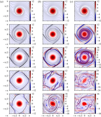
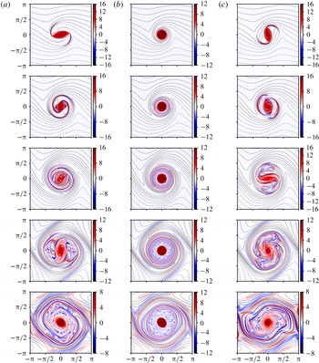
, namely 0.125, 0.5 and 2, corresponding to a weak, moderate and strong magnetic field (at full intensity). For the initially Gaussian vortex, figure 1 shows the evolution of the vorticity field (colour) overlaid with field lines (contours of
 $A+B_{0}y$
) for the three values of
 $\unicode[STIX]{x1D6FE}$
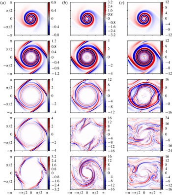
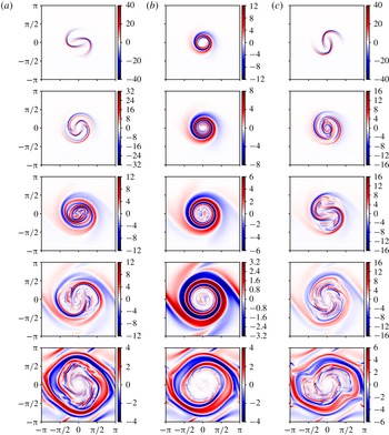
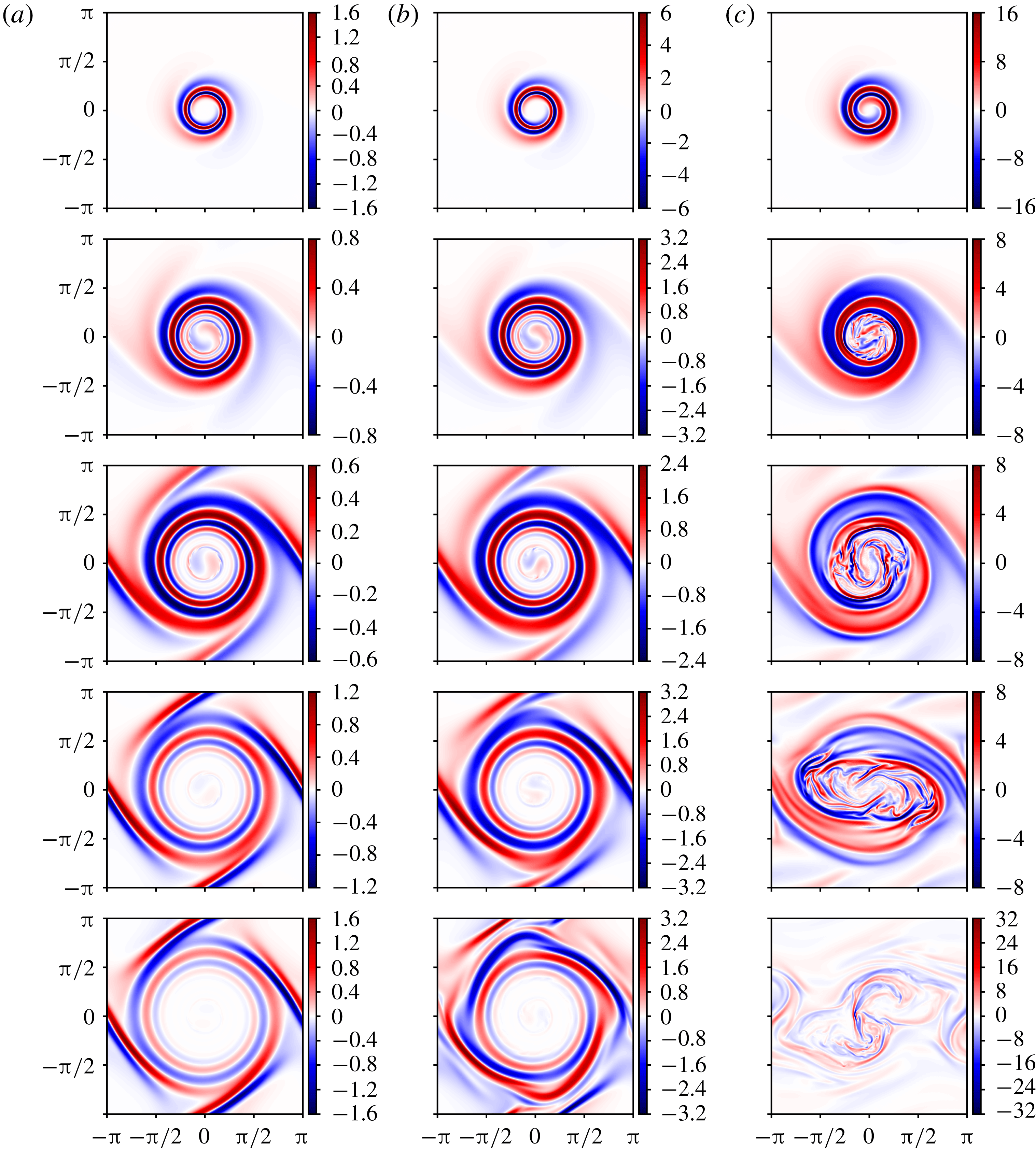
(increasing from left to right). The corresponding current density is shown in figure 2.
Vorticity
 $\unicode[STIX]{x1D714}(\boldsymbol{x},t)$
and magnetic field lines at times
 $t=2$
, 6, 12, 18 and 25 (top to bottom) for an initially Gaussian vortex and for
 $\unicode[STIX]{x1D6FE}=0.125$
, 0.5 and 2 (a–c). The vorticity colour bar is indicated next to each image. The contour interval for
 $A+B_{0}y$
is 0.005, 0.02 and 0.08 (left to right).

As in figure 1, but for the current density
 $j(\boldsymbol{x},t)$
.
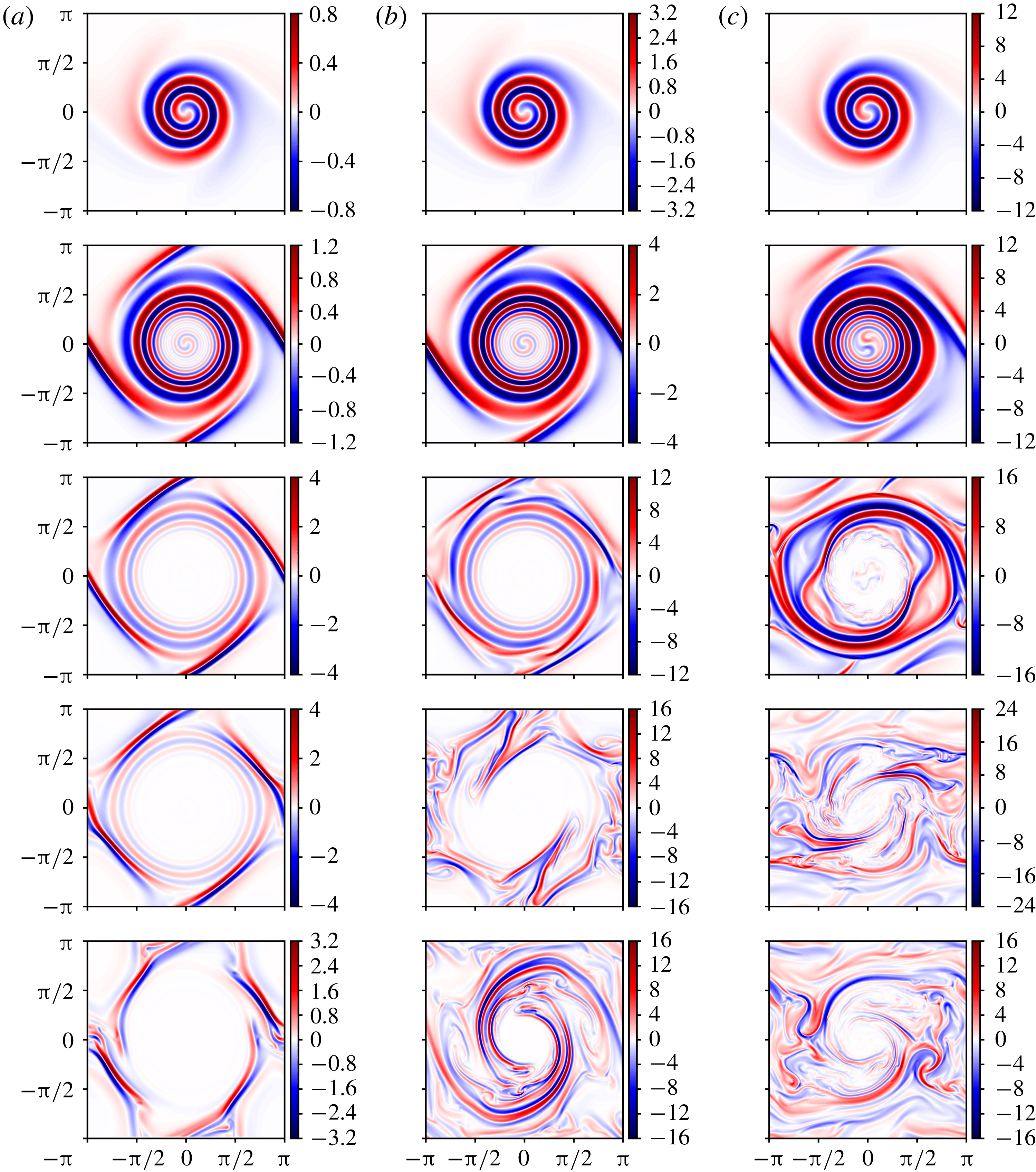
In figures 1(a) and 2(a), the weak field has no discernible impact on the vortex, which remains approximately circular and undiminished throughout the evolution. The field itself is twisted rapidly and field lines are broken by the magnetic diffusivity, leading to an expanding region of nearly zero field – this is the classic ‘flux expulsion’ phenomenon first described by Weiss (Reference Weiss1966). Note that the current sheets and strong field gradients developing in the periphery are a consequence of periodicity; otherwise the region of nearly zero field would continue expanding. These strong gradients generate vorticity, which subsequently destabilises and disrupts the field in this region, away from the central vortex.
In figures 1(b) and 2(b) for a stronger initial field, the initial evolution is closely similar. Now, however, a weak spiral pattern in vorticity is generated by the tightening field gradients before diffusion erases them. Moreover, the outer gradients induced by periodicity are much stronger and more disruptive at late times, distorting the vortex into an elliptical shape and eroding it. The expelled field in this case collapses back towards the vortex and strongly interacts with it at late times – again, here the later dynamics is a consequence of periodicity.
In figures 1(c) and 2(c) for the strongest initial field, again the early evolution is similar. Also, spiral vorticity generation occurs, but this time the vorticity becomes comparable with that in the core, and the alternating bands of vorticity destabilise by
 $t=12$
. The subsequent evolution is much more turbulent and noticeably affects the vortex core itself, causing strong distortion and a loss of symmetry at late times. In this case, the field is never fully expelled initially and the strong gradients collapse back more rapidly, leaving weaker gradients only in the vortex core. A slightly higher initial field strength (
 $\unicode[STIX]{x1D6FE}=2.5$
) leads to the complete destruction of the vortex by
 $t=25$
(not shown).
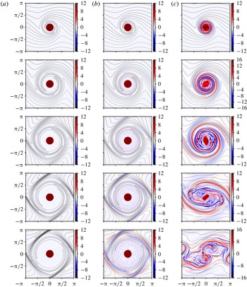
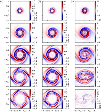
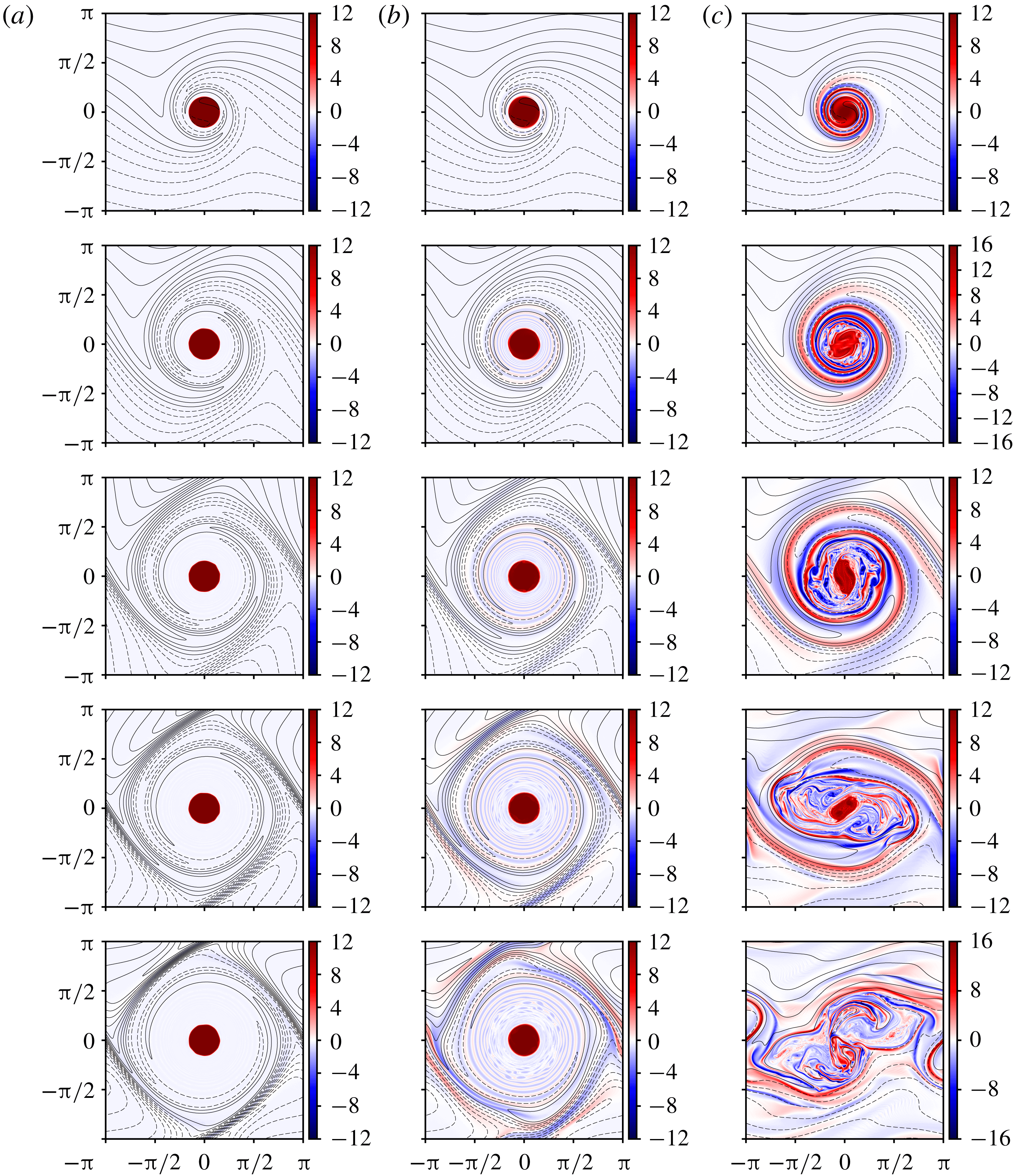
We now contrast the Gaussian vortex with a circular vortex patch of uniform initial vorticity. We choose the same
 $\unicode[STIX]{x1D6FF}$
and
 $\unicode[STIX]{x1D6FE}$
values so that any differences may be attributed to the initial vorticity profile. The vorticity (with superimposed field lines) and current density are illustrated in figures 3 and 4, respectively. Compared with figures 1 and 2, there are striking differences. First of all, in general, the magnetic field amplification is much stronger for the patch than for the Gaussian vortex, leading to greater disruption at late times and indeed vortex destruction for
 $\unicode[STIX]{x1D6FE}=2$
. In that case, the field is never expelled and interacts strongly with the vortex, ultimately pulling it apart and leaving intense current sheets where the vortex used to be. For moderate initial field strength (
 $\unicode[STIX]{x1D6FE}=0.5$
, figure 3
b), the vorticity filament spiral outside of the initial vortex destabilises, something only seen for
 $\unicode[STIX]{x1D6FE}=2$
in the case of the Gaussian vortex. Even for weak initial field (
 $\unicode[STIX]{x1D6FE}=0.125$
, figure 3
a), there is evidence that the field is disturbing the vortex boundary, which is no longer circular but more polygonal. Evidently, the less regular flow associated with the vortex patch, especially the discontinuity in shear at its edge, gives rise to a much stronger local interaction with the magnetic field. This is quantified below.
Vorticity
 $\unicode[STIX]{x1D714}(\boldsymbol{x},t)$
and magnetic field lines at times
 $t=2$
, 6, 12, 18 and 25 (top to bottom) for an initially uniform (Rankine) vortex and for
 $\unicode[STIX]{x1D6FE}=0.125$
, 0.5 and 2 (a–c). The vorticity colour bar is indicated next to each image. The contour interval for
 $A+B_{0}y$
is 0.005, 0.02 and 0.08 (left to right).
As in figure 3, but for the current density
 $j(\boldsymbol{x},t)$
.
3.3 Quantitative results
We next discuss various quantitative aspects of the flow evolution before developing a scaling theory to explain the results. An important diagnostic is the vortex circulation
 $\unicode[STIX]{x1D6E4}$
defined in (2.5), in particular its rate of change
 $\text{d}\unicode[STIX]{x1D6E4}/\text{d}t$
, which may be computed using (2.6). The circulation changes only as a result of the magnetic field, and given that field lines are twisted by the vortex, we expect a priori that the associated tension will act to slow the vortex rotation, reducing its circulation. At least, this should happen initially.
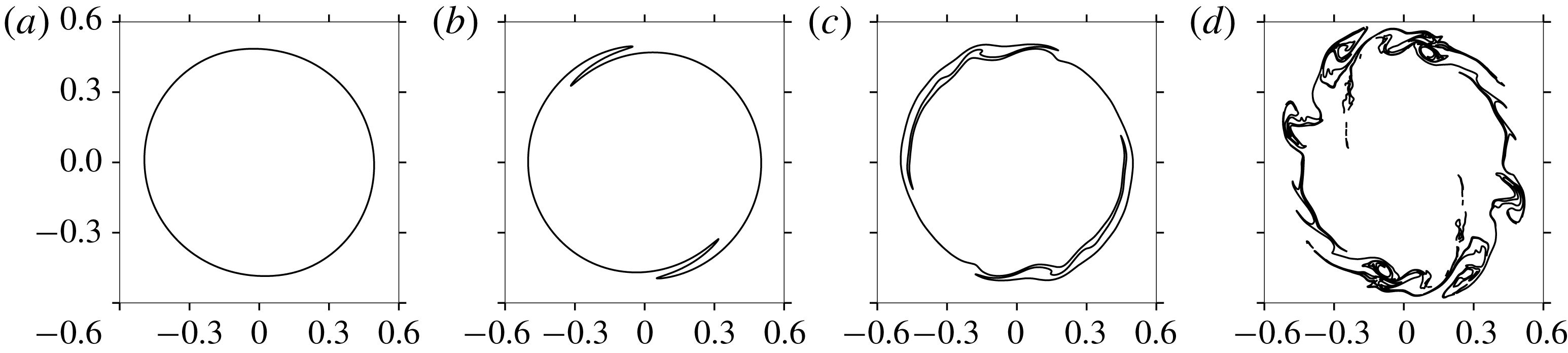
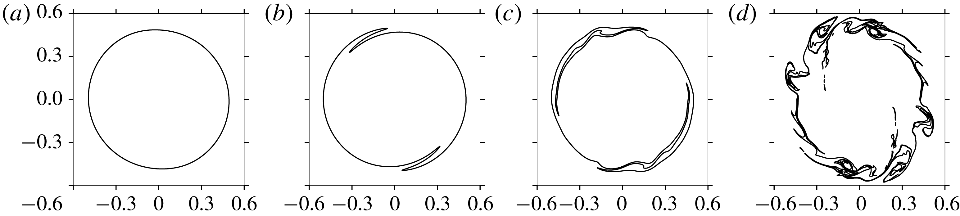
The material contour (or contours) belonging to the original circular tracer contour at times
 $t=5$
, 10, 15 and 20 (a–d) for the Gaussian vortex case with
 $\unicode[STIX]{x1D6FF}=0.0125$
(
 $n_{g}=1024$
) and
 $\unicode[STIX]{x1D6FE}=2$
. Only the inner portion of the flow domain is shown.
We compute the circulation using a material contour
 ${\mathcal{C}}$
that is initially a circle of radius
 $R$
centred at the origin. The contour is evolved in just the same way as the vorticity contours, except that it is never rebuilt. It may generally distort and even split into various parts, but at all stages the collection of contours belonging to the original contour is used in the contour integrations required in (2.5) and (2.6). A more extreme example showing how
 ${\mathcal{C}}$
may distort is provided in figure 5. Here, at late times,
 ${\mathcal{C}}$
splits into many parts, though most of these are very small. Nonetheless, accurate contour integration can be performed around such contours. Here, we use two-point Gaussian quadrature and the actual curved shape of the contour between successive nodes. At the evaluation points, the fields such as
 $\boldsymbol{u}$
and
 $j$
are interpolated from nearby gridded values using bilinear interpolation. This quadrature and the interpolation are both consistent with the cubic order of accuracy of the contour representation in the numerical method employed.
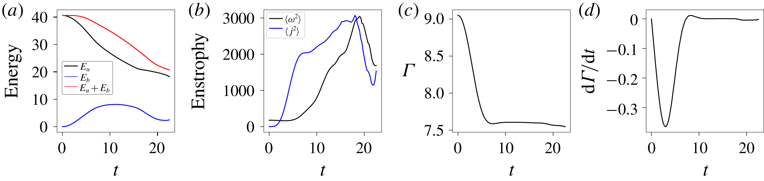
Time evolution of various diagnostics for the Gaussian vortex case with
 $\unicode[STIX]{x1D6FF}=0.0125$
and
 $\unicode[STIX]{x1D6FE}=2$
, i.e. as in figure 5. From (a) to (d), we show energy, enstrophy, circulation and the circulation rate of change. See text for details.
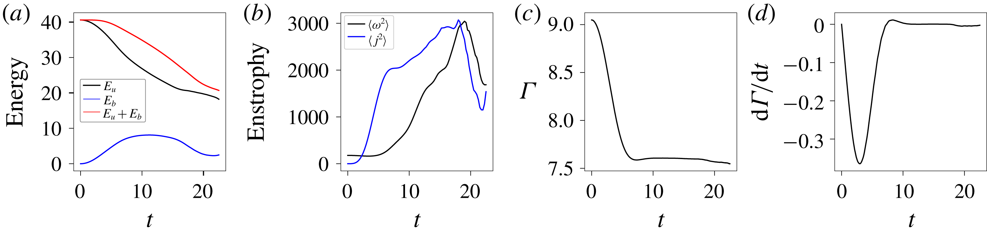
Figure 6 shows
 $\unicode[STIX]{x1D6E4}$
and
 $\text{d}\unicode[STIX]{x1D6E4}/\text{d}t$
along with other important diagnostics for an initially Gaussian vortex when
 $\unicode[STIX]{x1D6FF}=0.0125$
and
 $\unicode[STIX]{x1D6FE}=2$
. Figure 6 also shows the hydrodynamic (or kinetic) and magnetic energy components, respectively,
 $$\begin{eqnarray}E_{u}=\frac{1}{2}\int _{-\unicode[STIX]{x03C0}}^{\unicode[STIX]{x03C0}}\int _{-\unicode[STIX]{x03C0}}^{\unicode[STIX]{x03C0}}|\boldsymbol{u}|^{2}\,\text{d}x\,\text{d}y\quad \text{and}\quad E_{b}=\frac{1}{2}\int _{-\unicode[STIX]{x03C0}}^{\unicode[STIX]{x03C0}}\int _{-\unicode[STIX]{x03C0}}^{\unicode[STIX]{x03C0}}|\unicode[STIX]{x1D735}A|^{2}\,\text{d}x\,\text{d}y,\end{eqnarray}$$
together with the total energy
 $E=E_{u}+E_{b}$
, as well as the hydrodynamic and magnetic ‘enstrophies’
 $\langle \unicode[STIX]{x1D714}^{2}\rangle$
and
 $\langle \,j^{2}\rangle$
, here defined as the domain mean values of
 $\unicode[STIX]{x1D714}^{2}$
and
 $j^{2}$
. Note that
 $E_{b}$
does not include the constant part of the magnetic energy associated with the initial mean magnetic field
 $B_{0}\hat{\boldsymbol{e}}_{x}$
. For the hydrodynamic case, the enstrophy
 $\langle \unicode[STIX]{x1D714}^{2}\rangle$
is conserved in the absence of viscosity; whilst for the ideal MHD case, the total energy
 $E$
(magnetic plus kinetic) is conserved, whilst the enstrophy is not. Note that, in this limit of zero magnetic diffusivity,
 $\langle \,j^{2}\rangle$
is not conserved; however, any functional of
 $A+B_{0}y$
is, since this field is materially conserved (and the flow is incompressible). However, this limit is not relevant for the present purposes and is likely to be mathematically ill-posed (Cao et al.
Reference Cao, Wu and Yuan2017).
The case illustrated in figure 6 is broadly representative of all simulations conducted. All share similar trends, albeit with different amplitudes and time scales. The kinetic energy decays while the magnetic energy grows non-diffusively at first, as evidenced by the conservation of the total energy at early times (red curve). As field gradients increase, magnetic diffusion and the Lorentz force begin to act, ultimately halting the growth in magnetic energy and inducing decay at later times. Note that the background magnetic energy
 $\bar{E}_{b}=(1/2)B_{0}^{2}(2\unicode[STIX]{x03C0})^{2}$
, which is ignored in
 $E_{b}$
, is typically small compared with the maximum
 $E_{b}$
observed. In this example,
 $\bar{E}_{b}\approx 0.117$
, which is less than 2 % of the maximum
 $E_{b}$
. The decay in kinetic energy
 $E_{u}$
is consistent with the action of the field, forcing the vortex to slow down as field lines twist. Only the breaking of field lines by the diffusion allows the vortex to survive.
Regarding the enstrophy and current density, the mean-square current density
 $\langle \,j^{2}\rangle$
initially grows rapidly until approximately
 $t=6$
, during which time the hydrodynamic enstrophy
 $\langle \unicode[STIX]{x1D714}^{2}\rangle$
weakly decays. Over this period, the vortex is mainly slowing down as it twists magnetic field lines. Around
 $t=6$
, magnetic diffusion begins to act strongly, expelling the field from the vortex core and its immediate vicinity. After this time,
 $\langle \,j^{2}\rangle$
grows more slowly but
 $\langle \unicode[STIX]{x1D714}^{2}\rangle$
begins to grow rapidly, reaching a value more than 17 times its initial value by
 $t=19$
before subsequently decaying. This growth is due to the vorticity production by the strong current sheets created in the periphery of the vortex, primarily around and after
 $t=6$
(cf. figure 2
c). Only when these sheets begin to decay significantly at late times does
 $\langle \unicode[STIX]{x1D714}^{2}\rangle$
begin to decay. This decay is not inviscid: numerical dissipation acting at scales well below the grid scale are sufficient to cause a strong decay when
 $\unicode[STIX]{x1D714}$
develops extensive fine-scale structure in the form of filaments or sheets.
The time evolution of the circulation
 $\unicode[STIX]{x1D6E4}$
and its rate of change
 $\text{d}\unicode[STIX]{x1D6E4}/\text{d}t$
are consistent with the foregoing description. Up to
 $t=6$
, the circulation continually decreases as the twisting magnetic field lines slow the vortex rotation. The slowing decay after
 $t=3$
indicates that magnetic diffusion is already breaking field lines and thus reducing the impact on the vortex. After
 $t=6$
, the circulation remains roughly constant (with a small rebound just after
 $t=6$
), despite the continued vorticity production beyond the vortex core. This is because the contour
 ${\mathcal{C}}$
around which the circulation is computed remains near the centre of the domain, as shown previously in figure 5. Notably, since the circulation of the entire domain must be zero in a doubly periodic domain (by Stokes’ theorem), then the total circulation outside of
 ${\mathcal{C}}$
is just
 $-\unicode[STIX]{x1D6E4}$
. In particular, this means that, despite the intense vorticity production occurring beyond the vortex core, the net change in total vorticity there is small after
 $t=6$
.
3.4 Scaling theory
We next focus on the behaviour of
 $\text{d}\unicode[STIX]{x1D6E4}/\text{d}t$
, in particular how its evolution depends on the parameters
 $\unicode[STIX]{x1D6FF}$
and
 $\unicode[STIX]{x1D6FE}$
as well as on the initial vorticity distribution. Given the crucial role played by the magnetic diffusivity, we expect the flow to evolve on an appropriate diffusive time scale, which may (and does) depend on the initial vorticity distribution. Moreover, the amplitude of
 $\text{d}\unicode[STIX]{x1D6E4}/\text{d}t$
is expected to increase as
 $\unicode[STIX]{x1D6FF}$
and
 $\unicode[STIX]{x1D6FE}$
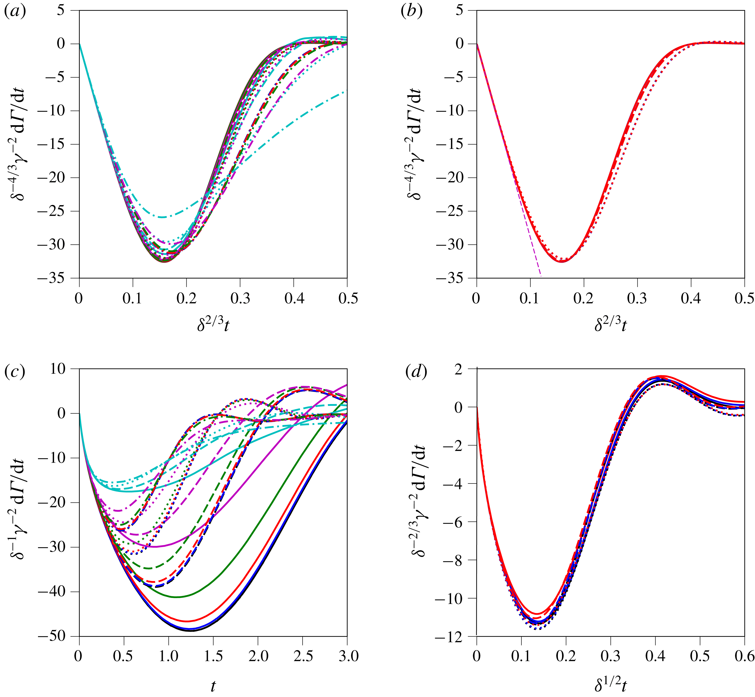
increase. Figure 7 summarises all of the results, both for the Gaussian vortex (a,b) and for the circular vortex patch (c,d), for four values of
 $\unicode[STIX]{x1D6FF}\in [0.0125,0.1]$
differing by factors of two, and for six values of
 $\unicode[STIX]{x1D6FE}\in [0.0625,2]$
also differing by factors of two.
Scaled forms of
 $\text{d}\unicode[STIX]{x1D6E4}/\text{d}t$
, as indicated, for
 $\unicode[STIX]{x1D6FF}=0.0125$
, 0.025, 0.05 and 0.1, and for
 $\unicode[STIX]{x1D6FE}=0.0625$
, 0.125, 0.25, 0.5, 1 and 2. The values of
 $\unicode[STIX]{x1D6FF}$
are distinguished by line style: solid, dashed, dotted and dash-dotted, respectively. The values of
 $\unicode[STIX]{x1D6FE}$
are distinguished by colour: black, blue, red, green, magenta and cyan, respectively. Panels (a,b) pertain to the initially Gaussian vortex, while (c,d) pertain to the initially circular vortex patch. The straight dashed magenta line in (b) is the fit to (3.8). See text for further details.
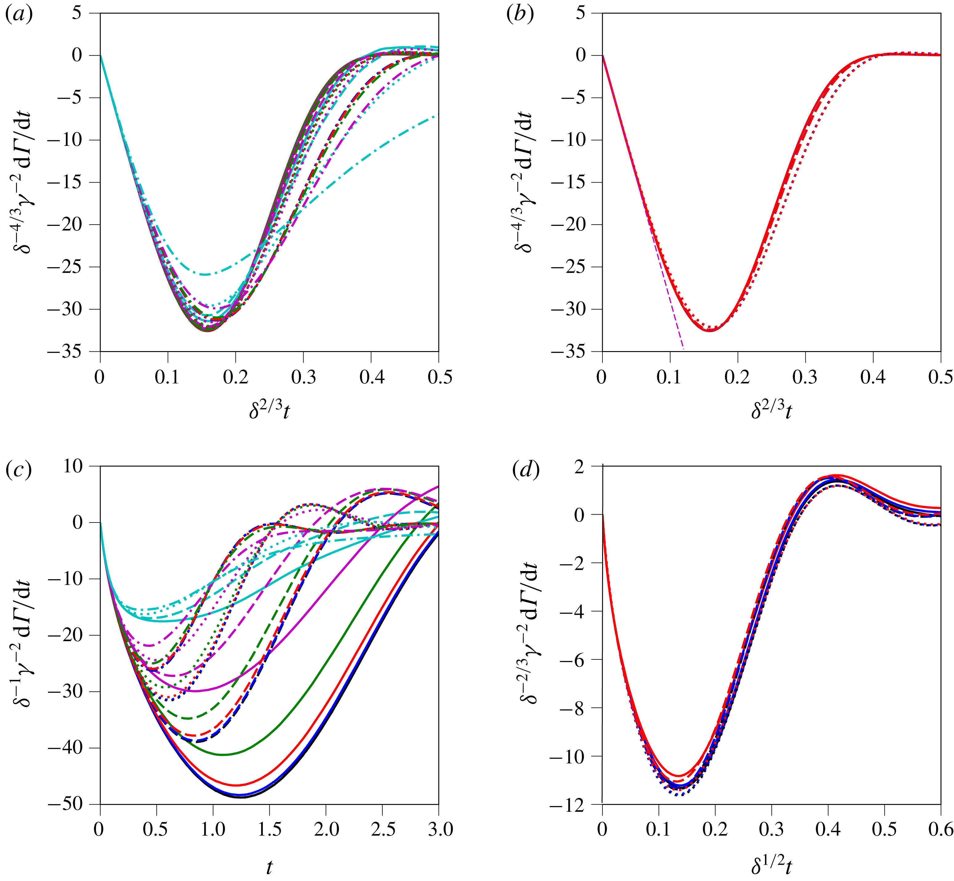
First consider figure 7(a,b) for the initially Gaussian vortex. Panel (b) merely shows a restricted set of parameters, namely the three smallest
 $\unicode[STIX]{x1D6FF}$
values and the three smallest
 $\unicode[STIX]{x1D6FE}$
values. This is done to show just how well the curves collapse for small
 $\unicode[STIX]{x1D6FF}$
and
 $\unicode[STIX]{x1D6FE}$
, where one might expect a scaling theory to apply. The results show a clear dependence on the scaled time
 $\unicode[STIX]{x1D6FF}^{2/3}t$
, rather than the
 $\unicode[STIX]{x1D6FF}^{2}t$
dependence one might expect for pure diffusive decay. This is due to the spiral wind-up of the magnetic field (which at small
 $\unicode[STIX]{x1D6FE}$
behaves like a passive tracer), accelerating the diffusive decay (
 $\propto \unicode[STIX]{x1D702}^{1/3}$
), as originally shown by Bajer et al. (Reference Bajer, Bassom and Gilbert2001). The quadratic dependence of
 $\text{d}\unicode[STIX]{x1D6E4}/\text{d}t$
on
 $\unicode[STIX]{x1D6FE}$
is just a consequence of the form of the integrand in (2.6), where a quadratic product of quantities proportional to the magnetic field appears.
The dependence on
 $\unicode[STIX]{x1D6FF}^{4/3}$
may be explained by considering the early-time evolution of
 $\text{d}\unicode[STIX]{x1D6E4}/\text{d}t$
and using Moffatt’s approximate inviscid solution for
 $A$
,
 $$\begin{eqnarray}A(r,\unicode[STIX]{x1D703},t)=B_{0}r[\sin (\unicode[STIX]{x1D703}-\bar{\unicode[STIX]{x1D6FA}}t)-\sin \unicode[STIX]{x1D703}]\end{eqnarray}$$
(Moffatt Reference Moffatt1983). This assumes that the background flow is steady and axisymmetric, with angular frequency
 $\bar{\unicode[STIX]{x1D6FA}}(r)$
a function of
 $r$
only, and moreover that
 $\unicode[STIX]{x1D6FE}\ll 1$
. This solution directly follows from (2.3), neglecting
 $\unicode[STIX]{x1D702}$
, and can be seen most easily by recognising that the total potential
 $\tilde{A}=A+B_{0}y$
satisfies (for a steady axisymmetric flow)
 $$\begin{eqnarray}\tilde{A}_{t}+\bar{\unicode[STIX]{x1D6FA}}\tilde{A}_{\unicode[STIX]{x1D703}}=0,\end{eqnarray}$$
implying
 $\tilde{A}=F(r,\unicode[STIX]{x1D703}-\bar{\unicode[STIX]{x1D6FA}}t)$
for some function
 $F$
. This function is determined from the initial conditions,
 $\tilde{A}(r,\unicode[STIX]{x1D703},0)=B_{0}y=B_{0}r\sin \unicode[STIX]{x1D703}$
, giving
 $F(r,\unicode[STIX]{x1D703})=B_{0}r\sin \unicode[STIX]{x1D703}$
, from which (3.2) follows. Now, to estimate
 $\text{d}\unicode[STIX]{x1D6E4}/\text{d}t$
at early times (before diffusion has a chance to act significantly), we also need the current density
 $j$
. Using Moffatt’s solution (3.2) for
 $A$
, we find
 $$\begin{eqnarray}j(r,\unicode[STIX]{x1D703},t)=B_{0}t(r\bar{\unicode[STIX]{x1D6FA}}_{rr}+3\bar{\unicode[STIX]{x1D6FA}}_{r})\cos (\unicode[STIX]{x1D703}-\bar{\unicode[STIX]{x1D6FA}}t)+B_{0}t^{2}r\bar{\unicode[STIX]{x1D6FA}}_{r}^{2}\sin (\unicode[STIX]{x1D703}-\bar{\unicode[STIX]{x1D6FA}}t).\end{eqnarray}$$
Using this and
 $\tilde{A}_{\unicode[STIX]{x1D703}}=B_{0}r\cos (\unicode[STIX]{x1D703}-\bar{\unicode[STIX]{x1D6FA}}t)$
in (2.6) written using the parametrisation
 $\unicode[STIX]{x1D703}$
, we obtain after elementary integration
 $$\begin{eqnarray}\frac{\text{d}\unicode[STIX]{x1D6E4}}{\text{d}t}=B_{0}^{2}\unicode[STIX]{x03C0}t(r^{2}\bar{\unicode[STIX]{x1D6FA}}_{rr}+3r\bar{\unicode[STIX]{x1D6FA}}_{r})_{r=R}\end{eqnarray}$$
(the
 $t^{2}$
term integrates to zero). But for the Gaussian vortex,
 $$\begin{eqnarray}\bar{\unicode[STIX]{x1D6FA}}(r)=\unicode[STIX]{x1D714}_{max}\frac{R^{2}}{r^{2}}(1-\text{e}^{-r^{2}/2R^{2}}).\end{eqnarray}$$
After some algebra, one may show that
 $$\begin{eqnarray}(r^{2}\bar{\unicode[STIX]{x1D6FA}}_{rr}+3r\bar{\unicode[STIX]{x1D6FA}}_{r})_{r=R}=-\unicode[STIX]{x1D714}_{max}\text{e}^{-1/2}.\end{eqnarray}$$
Next, using
 $B_{0}=\unicode[STIX]{x1D6FF}\unicode[STIX]{x1D6FE}U_{0}={\textstyle \frac{1}{2}}\unicode[STIX]{x1D6FF}\unicode[STIX]{x1D6FE}\unicode[STIX]{x1D714}_{0}R$
from (2.4) in (3.5) together with
 $\unicode[STIX]{x1D714}_{max}=\unicode[STIX]{x1D714}_{0}/(2(1-\text{e}^{-1/2}))$
, we obtain the following explicit prediction for
 $\text{d}\unicode[STIX]{x1D6E4}/\text{d}t$
:
 $$\begin{eqnarray}\frac{\text{d}\unicode[STIX]{x1D6E4}}{\text{d}t}=-\unicode[STIX]{x1D6FF}^{2}\unicode[STIX]{x1D6FE}^{2}\frac{\unicode[STIX]{x03C0}\unicode[STIX]{x1D714}_{0}^{3}R^{2}}{8(\text{e}^{1/2}-1)}t.\end{eqnarray}$$
This is plotted as the straight dashed magenta line in figure 7(b). It coincides with the initially linear decrease in
 $\text{d}\unicode[STIX]{x1D6E4}/\text{d}t$
. Moreover, it shows that
 $\unicode[STIX]{x1D6FF}^{-4/3}\unicode[STIX]{x1D6FE}^{-2}\,\text{d}\unicode[STIX]{x1D6E4}/\text{d}t$
should be proportional to the scaled time
 $\unicode[STIX]{x1D6FF}^{2/3}t$
, as observed. At later times,
 $\text{d}\unicode[STIX]{x1D6E4}/\text{d}t$
is affected by magnetic diffusion, neglected here. This arrests the change in circulation, ultimately reducing it to near zero at late times. This scaling is consistent with the early-time behaviour described by Gilbert et al. (Reference Gilbert, Mason and Tobias2016).
Next consider panels figure 7(c,d) for the circular vortex patch. In panel (c), all of the results are plotted versus the unscaled time
 $t$
but
 $\text{d}\unicode[STIX]{x1D6E4}/\text{d}t$
is scaled in such a way that the very early-time behaviour is closely similar: all 24 curves lie on top of each other for
 $t<0.2$
. In panel (d), we show that, by plotting
 $\text{d}\unicode[STIX]{x1D6E4}/\text{d}t$
versus the scaled time
 $\unicode[STIX]{x1D6FF}^{1/2}t$
and appropriately scaling
 $\text{d}\unicode[STIX]{x1D6E4}/\text{d}t$
, the curves nearly collapse onto a single curve. Here, again, only the three smallest
 $\unicode[STIX]{x1D6FF}$
values and the three smallest
 $\unicode[STIX]{x1D6FE}$
values are plotted. The collapse is not as good as for the Gaussian vortex in figure 7(b), but nonetheless extends well into the evolution, including the rebound after
 $\unicode[STIX]{x1D6FF}^{1/2}t=0.35$
(which is much stronger than seen for the Gaussian vortex).
From the earliest time, diffusion plays an important role, and hence the inviscid solution presented above for the Gaussian vortex does not apply. Equation (3.5) is problematic for the vortex patch, as the radial function there equals
 $-\unicode[STIX]{x1D714}_{0}R\unicode[STIX]{x1D6FF}(r-R)$
, where here
 $\unicode[STIX]{x1D6FF}(s)$
is Dirac’s delta function. In reality,
 $j$
immediately diffuses, and qualitatively should exhibit a
 $1/\sqrt{\unicode[STIX]{x1D702}t}$
time dependence at
 $r=R$
based on the solution to the heat equation. This would imply
 $$\begin{eqnarray}\frac{\text{d}\unicode[STIX]{x1D6E4}}{\text{d}t}\sim -B_{0}^{2}t\frac{\unicode[STIX]{x1D714}_{0}R}{\sqrt{\unicode[STIX]{x1D702}t}}\sim -\unicode[STIX]{x1D6FF}\unicode[STIX]{x1D6FE}^{2}\unicode[STIX]{x1D714}_{0}^{2}R^{2}\sqrt{\unicode[STIX]{x1D714}_{0}t}\end{eqnarray}$$
(the constant of proportionality based on the solution of the heat equation is
 $\sqrt{\unicode[STIX]{x03C0}}/8$
). While this qualitatively explains the observed nonlinear time dependence in
 $\text{d}\unicode[STIX]{x1D6E4}/\text{d}t$
in figure 7(a,b), it represents only a crude fit. This is probably due to assuming that
 $j$
evolves according to the heat equation while using the inviscid solution for
 $A$
. Nonetheless, (3.9) explains the dependence on
 $\unicode[STIX]{x1D6FF}\unicode[STIX]{x1D6FE}^{2}$
exhibited in figure 7(c).
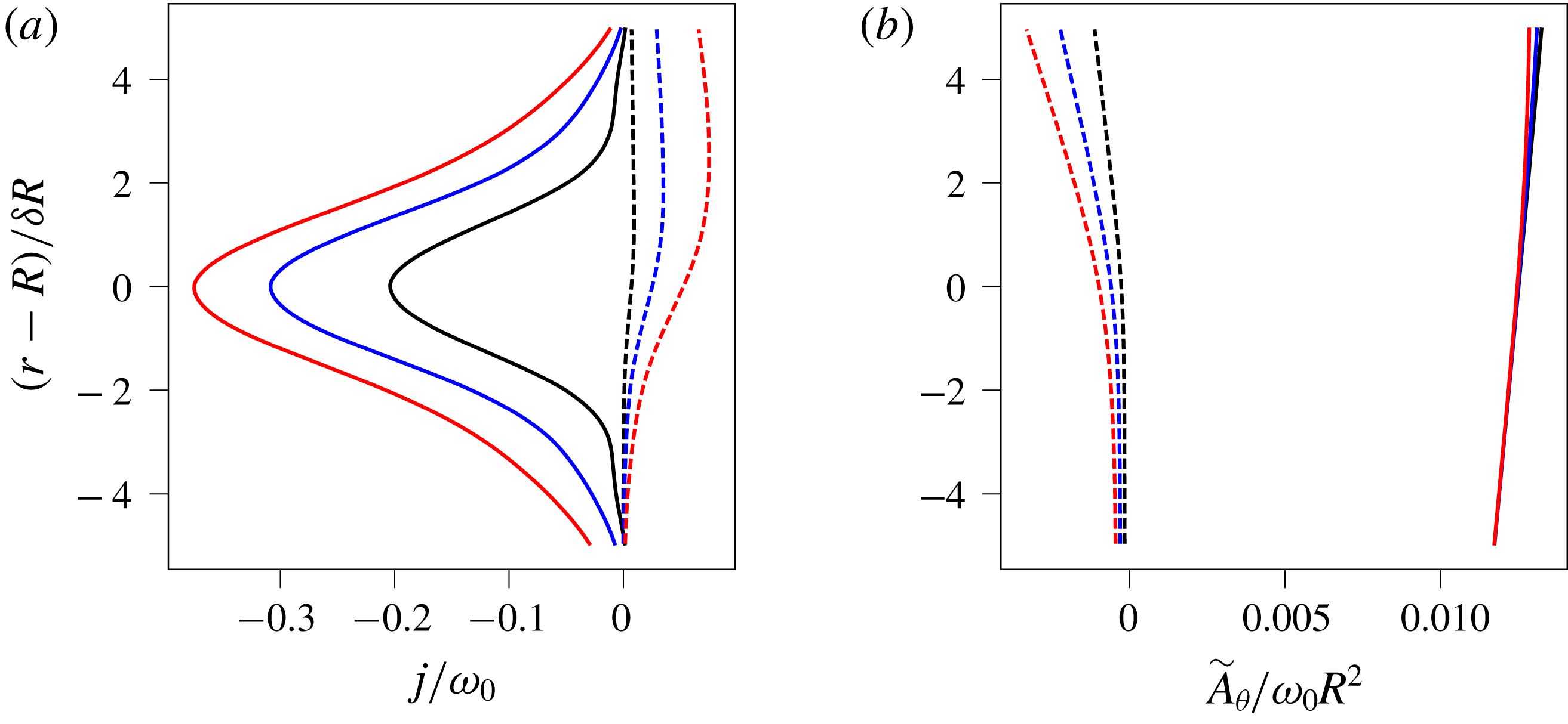
Scaled radial dependences of (a)
 $j$
and (b)
 $\tilde{A}_{\unicode[STIX]{x1D703}}$
near the edge of a circular vortex patch, projected onto the cosine and sine azimuthal modes (solid and dashed, respectively) at times
 $t=0.1$
(black), 0.2 (blue) and 0.3 (red). These results are derived from a simulation starting from a circular vortex patch with
 $\unicode[STIX]{x1D6FF}=0.0125$
and
 $\unicode[STIX]{x1D6FE}=1$
.
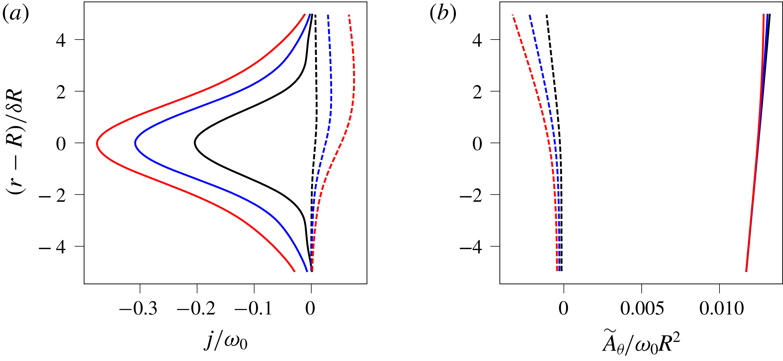
The actual radial cross-sections of
 $j$
and
 $\tilde{A}_{\unicode[STIX]{x1D703}}$
near the vortex edge, projected onto the
 $\cos (\unicode[STIX]{x1D703}-\bar{\unicode[STIX]{x1D6FA}}t)$
and
 $\sin (\unicode[STIX]{x1D703}-\bar{\unicode[STIX]{x1D6FA}}t)$
azimuthal modes, are shown in figure 8. We find that the cosine projection of
 $j$
indeed exhibits a roughly Gaussian dependence on
 $r-R$
, while the cosine projection of
 $\tilde{A}_{\unicode[STIX]{x1D703}}$
varies only weakly across
 $r=R$
. However, the sine projection of
 $\tilde{A}_{\unicode[STIX]{x1D703}}$
is a diffusive effect, and spoils any simple theoretical prediction for
 $\text{d}\unicode[STIX]{x1D6E4}/\text{d}t$
.
Finally, we remark that
 $|\text{d}\unicode[STIX]{x1D6E4}/\text{d}t|$
grows to much larger values for the initially circular patch than for the Gaussian. As an example, for the smallest
 $\unicode[STIX]{x1D6FF}$
and
 $\unicode[STIX]{x1D6FE}$
values, the ratio in the maximum values of
 $|\text{d}\unicode[STIX]{x1D6E4}/\text{d}t|$
is 6.45. The circular patch therefore is much more strongly affected by the magnetic field than the Gaussian vortex.
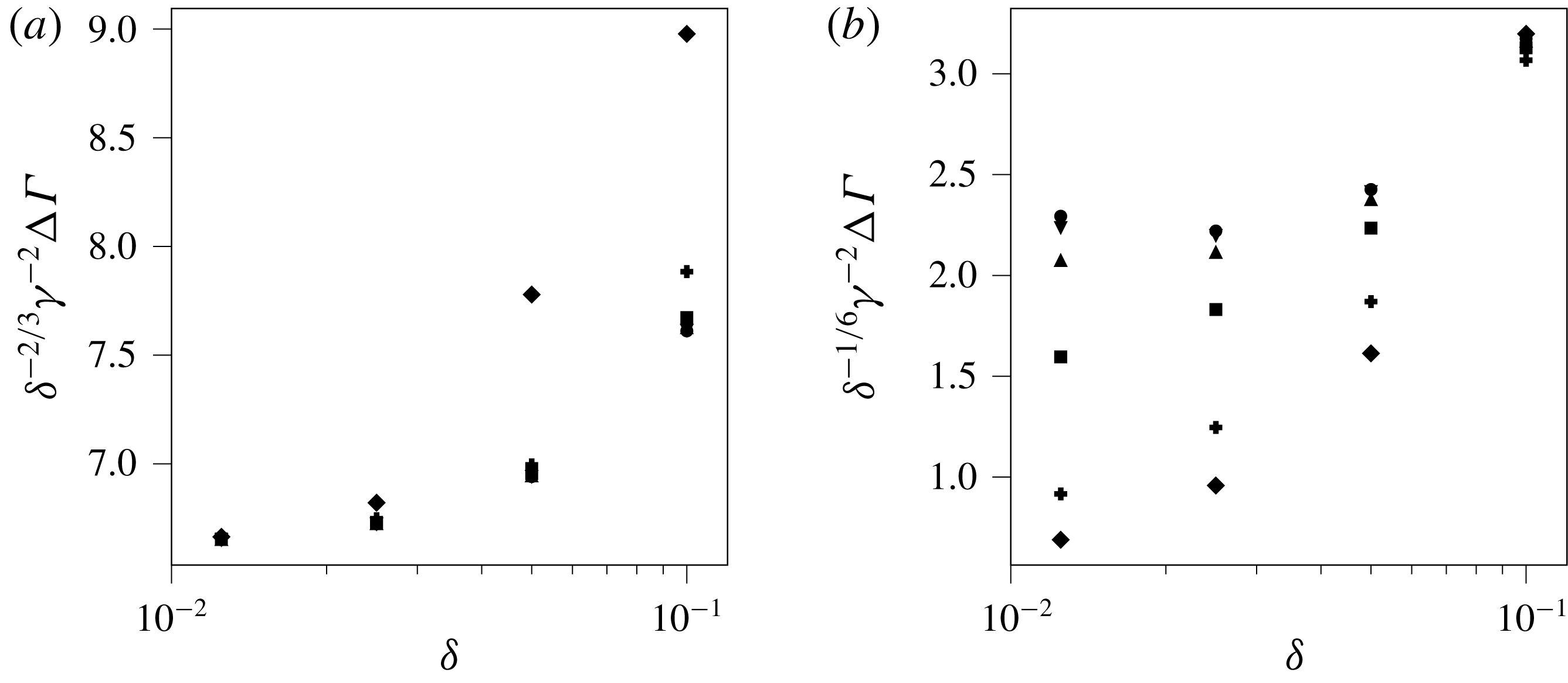
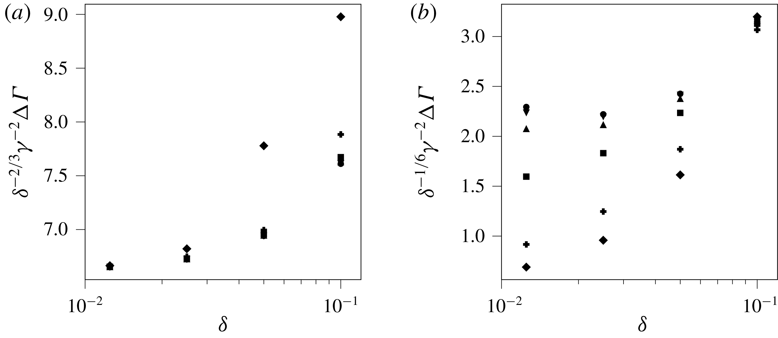
Scaled net reduction in circulation for (a) the initial Gaussian vortex and (b) the initial circular vortex patch, as a function of
 $\unicode[STIX]{x1D6FF}$
. The symbols indicate the value of
 $\unicode[STIX]{x1D6FE}$
. In order of increasing
 $\unicode[STIX]{x1D6FE}$
, the symbols are circle, triangle pointing down, triangle pointing up, square, plus and diamond.
In nearly all simulations conducted for either vortex profile, the circulation
 $\unicode[STIX]{x1D6E4}$
decreases and levels off at a nearly constant value, particularly for small
 $\unicode[STIX]{x1D6FF}$
and
 $\unicode[STIX]{x1D6FE}$
(when the vortex is not greatly disrupted). The above scaling results can be used to estimate the total reduction in circulation
 $\unicode[STIX]{x0394}\unicode[STIX]{x1D6E4}$
. For the initially Gaussian vortex, integrating
 $-\text{d}\unicode[STIX]{x1D6E4}/\text{d}t$
from
 $t=0$
to
 $t\sim \unicode[STIX]{x1D6FF}^{-2/3}$
gives the estimate
 $\unicode[STIX]{x0394}\unicode[STIX]{x1D6E4}\sim \unicode[STIX]{x1D6FF}^{2/3}\unicode[STIX]{x1D6FE}^{2}$
. This is shown to predict well the actual change in circulation up to
 $t=0.5\unicode[STIX]{x1D6FF}^{-2/3}$
, as shown in figure 9(a). We stress that, in order to assess the ultimate role of the magnetic field in extracting circulation from the vortex – and therefore the ultimate fate of the vortex – the integrated effects of the Lorentz force must be calculated. The same integration for the patch to
 $t=0.6\unicode[STIX]{x1D6FF}^{-1/2}$
gives the estimate
 $\unicode[STIX]{x0394}\unicode[STIX]{x1D6E4}\sim \unicode[STIX]{x1D6FF}^{1/6}\unicode[STIX]{x1D6FE}^{2}$
. As seen in figure 9(b), this is not accurate, and suggests that the dependence on
 $\unicode[STIX]{x1D6FE}$
should be different. However, by log scaling the data and searching for best-fit curves, no simple relationship was found to collapse the data significantly better than shown in figure 9(b). The circular vortex patch is not nearly as simple as the Gaussian vortex.
3.5 Initially elliptical vortex patches
Vorticity
 $\unicode[STIX]{x1D714}(\boldsymbol{x},t)$
and magnetic field lines at times
 $t=1.5$
, 3, 6, 12 and 24 (top to bottom) for an initially elliptical vortex with
 $\unicode[STIX]{x1D706}=1/3$
, 1 and 3 (a–c). The vorticity colour bar is indicated next to each image. The contour interval for
 $A+B_{0}y$
is 0.04 in all images.

As in figure 10, but for the current density
 $j(\boldsymbol{x},t)$
.

We conclude this section by discussing the case of an initially elliptical vortex patch whose boundary is given by
 $$\begin{eqnarray}\frac{x^{2}}{a^{2}}+\frac{y^{2}}{b^{2}}=1,\end{eqnarray}$$
with
 $\sqrt{ab}=R$
so that it has the same area for all aspect ratios
 $\unicode[STIX]{x1D706}=b/a$
. One reason to study the ellipse is to understand the role of the threading of the field lines in the subsequent evolution of the vortex (see e.g. Keating et al.
Reference Keating, Silvers and Diamond2008). Would a vortex threaded by more field lines (
 $\unicode[STIX]{x1D706}>1$
) be more affected by the magnetic field than one which is threaded by fewer field lines (
 $\unicode[STIX]{x1D706}<1$
)? As a first qualitative view, figures 10 and 11 show the vorticity, field lines and current density for three ellipses, with
 $\unicode[STIX]{x1D706}=1/3$
(a),
 $\unicode[STIX]{x1D706}=1$
(b) and
 $\unicode[STIX]{x1D706}=3$
(c) – all for
 $\unicode[STIX]{x1D6FF}=0.025$
and
 $\unicode[STIX]{x1D6FE}=1$
. Note that an ellipse with
 $\unicode[STIX]{x1D706}<1/3$
or
 $\unicode[STIX]{x1D706}>3$
is linearly unstable in the absence of a magnetic field (Love Reference Love1893). Here the field acts to circularise the vortex. For both
 $\unicode[STIX]{x1D706}=1/3$
and
 $\unicode[STIX]{x1D706}=3$
, the impact of the field on the vortex is noticeably greater than for the circular vortex,
 $\unicode[STIX]{x1D706}=1$
. It appears that
 $\unicode[STIX]{x1D706}=3$
is most strongly affected, but the argument that more field lines initially threading the vortex has a greater impact is clearly not correct. The circular vortex is much less affected than the vortex with
 $\unicode[STIX]{x1D706}=1/3$
, which is threaded by the fewest field lines.
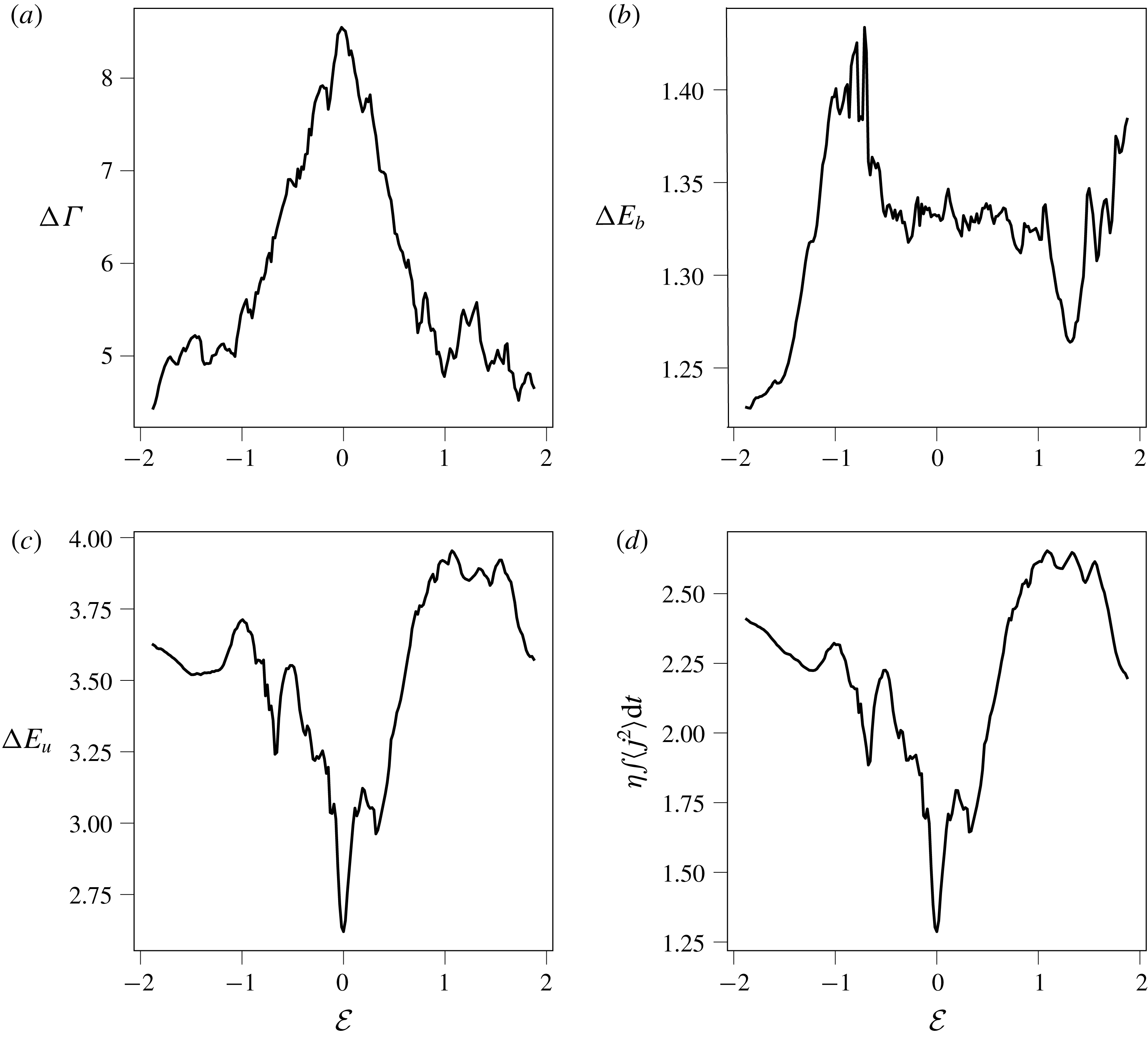
Accumulative diagnostics as a function of initial vortex eccentricity
 ${\mathcal{E}}$
. The diagnostics are computed over
 $0\leqslant t\leqslant 10$
and show (a) the net circulation reduction
 $\unicode[STIX]{x0394}\unicode[STIX]{x1D6E4}$
, (b) the net growth in magnetic energy
 $\unicode[STIX]{x0394}E_{b}$
, (c) the net decline in kinetic energy
 $\unicode[STIX]{x0394}E_{u}$
, and (d) the net magnetic dissipation
 $\unicode[STIX]{x1D702}\int _{0}^{10}\langle \,j^{2}\rangle \,\text{d}t$
. All simulations used the parameters
 $\unicode[STIX]{x1D6FF}=0.025$
and
 $\unicode[STIX]{x1D6FE}=1$
.

Instead, what appears to be important is the reach of the vortex in sweeping through the background magnetic field. Then, both small and large
 $\unicode[STIX]{x1D706}$
would exhibit a similar behaviour, and would be more affected than the circular vortex. This is borne out in figure 12, which plots various accumulative diagnostics for over 200 simulations varying the vortex eccentricity
 $$\begin{eqnarray}{\mathcal{E}}=\frac{1}{2}\left(\unicode[STIX]{x1D706}-\frac{1}{\unicode[STIX]{x1D706}}\right)\end{eqnarray}$$
over the range
 $-15/8\leqslant {\mathcal{E}}\leqslant 15/8$
, corresponding to
 $1/4<\unicode[STIX]{x1D706}<4$
. The results in figure 12 show that the circular vortex is clearly anomalous. Yet, the circular vortex also displays the greatest net reduction in circulation, despite keeping it shape. Ellipses retain their initial circulation better, not because they are less affected, but because the vorticity production near the vortex edge is different: both increases and decreases in vorticity occur within the vortex edge, whereas for a circular vortex only decreases occur. This can be seen to some extent in figure 10, where the plotted vorticity field levels are higher for both
 $\unicode[STIX]{x1D706}=1/3$
and
 $\unicode[STIX]{x1D706}=3$
than for
 $\unicode[STIX]{x1D706}=1$
. In short, the circulation changes occurring for distorted vortices are more complex but tend to be weaker than those occurring for an initially circular vortex.
Regarding the other diagnostics, there is very little dependence in the gain in magnetic energy on vortex eccentricity, but a significant dependence in the loss in kinetic energy. The initially circular vortex exhibits the least loss in kinetic energy, consistent with the images in figure 10, where the flow surrounding the vortex is generally much less agitated compared with the elliptical cases. Finally, the net magnetic dissipation is also weakest for the initially circular vortex, consistent with the generally weaker field of current density seen in the middle panels of figure 11.
Despite the fact that the ellipse is unstable for
 $\unicode[STIX]{x1D706}<1/3$
or
 $\unicode[STIX]{x1D706}>3$
in the absence of a magnetic field, the effect of the magnetic field in the examples shown (which here is not a weak effect) dominates the flow evolution, rapidly causing the vortex to become more circular in form. A weaker magnetic field might allow a competition between the hydrodynamic instability and the action of the field, but this is beyond the scope of the present study.
4 Conclusions and future work
In this paper we have examined the role of a weak magnetic field in modifying Kelvin’s circulation theorem in two-dimensional MHD at low magnetic Prandtl number
 $Pm$
. The circulation of the velocity field is a materially conserved quantity in hydrodynamics and plays a key role in determining the dynamics. That the magnetic field acts through the Lorentz force to destroy these conservation properties is well known, but quantifying the effect as a function of parameters (magnetic diffusion and field strength) has hitherto not been achieved. We consider three model flows that, in the absence of magnetic effects, remain exact stable solutions of the two-dimensional Euler equations; namely the Gaussian vortex, the circular vortex patch and the elliptical vortex patch.
As always in these situations, it appears as though the role of the magnetic field is more subtle than first (or even second) imagined. As noted by Gilbert et al. (Reference Gilbert, Mason and Tobias2016), the degree of circulation extracted from the vortices must be determined via integrating the effects of the Lorentz force over the entirety of the evolution, rather than by hypothesising balances of crude instantaneous measures of the Lorentz force, which will yield incorrect scalings. Furthermore, the roles of diffusion and Lorentz force depend on the initial configuration of the flow, with smooth vortices reacting rather differently from vortex patches.
While some degree of universality exists concerning the net circulation loss induced by a weak magnetic field for small magnetic diffusivity, the scalings found depend on both the vorticity profile and the vortex shape. As expected from the integral form of the rate of change of circulation, the circulation loss in all cases scales with the square of the field strength. The dependence on magnetic diffusivity is more subtle. There is a delicate interplay between diffusion and the shearing velocity field around a vortex, leading in many cases to accelerated diffusion, particularly in regions of high vorticity gradients. The situation is more complicated still for non-circular initial vortices. Perhaps counter-intuitively, the circular vortex leads to the greatest circulation loss; the more eccentric the initial vortex shape, the better the vortex preserves its initial circulation. This is explained by the fact that the tangentially varying velocity field around a non-circular vortex may locally lead to gains in circulation. These gains partially offset the losses, thereby leading to less circulation loss overall. The net magnetic dissipation is also smaller than for a circular vortex.
The dynamics and role of the magnetic field are different for high-
 $Rm$
fluids at low
 $Pm$
(such as astrophysical fluids) than they are for low-
 $Rm$
fluids at low
 $Pm$
(such as liquid metal experiments, and even some geophysical cases). The latter situation can be investigated in detail, as then the Lorentz force that breaks Kelvin’s theorem can be linearised about a background magnetic field. We are currently investigating the scalings that apply.
Although we have focused on simple models with no background rotation or (explicit) stratification, it is clear that the results can (and should) be extended to more geophysically and astrophysically relevant cases with these included. Simple extensions that should be (and are being) evaluated include incorporating rotation and stratification on both a
 $\unicode[STIX]{x1D6FD}$
-plane and a spherical surface. Here the key materially conserved quantity is the absolute (potential) vorticity, which includes the planetary and relative vorticity as well as density variations. Since material conservation of this scalar field has a significant effect on the dynamics (for example, being implicated in the formation of potential vorticity staircases; see e.g. Dritschel & McIntyre (Reference Dritschel and McIntyre2008)), then understanding the role of a magnetic field in modifying this conservation property is an important next step in understanding the dynamics of stably stratified magnetised environments (as described in Tobias (Reference Tobias, Soward, Jones, Hughes and Weiss2005)).
In flows where the background rotation and stratification are too weak to suppress three-dimensional turbulence, an interesting question arises concerning circulation conservation and vorticity dynamics more generally, especially in the presence of a magnetic field. The present study, while two-dimensional, emphasises the role of the magnetic field in taking the twist out of vorticity. The same effect should be present in a three-dimensional flow: the magnetic field is likely to suppress or slow down the growth of vorticity, possibly leading to greater regularity of the flow at small scales than in the purely hydrodynamic case. Tracking the changes in circulation around closed material curves in such flows is feasible, and is likely to reveal new insights into the small-scale nature of three-dimensional MHD turbulence.
Acknowledgements
P.H.D. and S.M.T. would like to acknowledge the support of the Festival de Théorie in Aix-en-Provence. Support for this research has come from the UK Engineering and Physical Sciences Research Council (grant no. EP/H001794/1).