1. Introduction
Transition to turbulence has been studied extensively in Newtonian channel flows due to its theoretical and practical importance. Previous numerical (Henningson, Lundbladh & Johansson Reference Henningson, Lundbladh and Johansson1993) and experimental (Breuer & Landahl Reference Breuer and Landahl1990) studies have examined the transition process starting from three-dimensional, initially localized disturbances to model generic perturbations in the flow. The early stages of transition can be explained by appealing to linear theory, but nonlinear effects ultimately become important and give way to the onset of turbulence. Both the linear and nonlinear stages can, however, deviate from the Newtonian behaviour when small quantities of polymers are introduced in the flow. Previous linear theory has focused on the stability of a laminar base state, while the nonlinear efforts have focused on fully turbulent flows due to the propensity of the polymer to reduce drag (Toms Reference Toms1948). The transition process, which includes the early linear dynamics and the subsequent nonlinear stages leading to turbulence, is examined herein using direct numerical simulations (DNS) of initially localized disturbances in polymeric channel flow.
1.1. Localized disturbance in Newtonian channel flow
Linear stability theory predicts that Poiseuille flow is stable up to a critical Reynolds number
 $\mathit{Re}=3848$
based on the channel half-height and the bulk velocity (Orszag Reference Orszag1971). By appealing to Squire’s theorem, at this critical Reynolds number the flow is unstable to a two-dimensional disturbance. Below the critical Reynolds number, while the flow does not possess any long-time instabilities, it can sustain transient energy amplification due to two- and three-dimensional disturbances of finite amplitude. Several growth mechanisms have been proposed for subcritical transition (Bayly, Orszag & Herbert Reference Bayly, Orszag and Herbert1988), and breakdown to turbulence in this regime is known as bypass transition (Orszag & Kells Reference Orszag and Kells1980): it bypasses the amplification of discrete instability waves seen in the natural transition route.
The evolution of a three-dimensional localized disturbance in channel flow has been studied by Henningson et al. (Reference Henningson, Lundbladh and Johansson1993). According to those authors, a disturbance of small amplitude undergoes linear growth due to the lift-up mechanism (Landahl Reference Landahl1975) during which the three-dimensionality of the disturbance causes a growth in the wall-normal perturbation vorticity. The disturbance is dominated by the streamwise velocity component, and starts to become elongated in the streamwise direction. However, the period of energy amplification is short lived and the flow returns to a laminar state due to viscous dissipation. For disturbances with larger initial amplitude, nonlinearity transfers energy from the initially localized disturbance into lower streamwise wavenumbers. Elongated vortices are formed close to the wall and are further intensified by the mean shear. These elongated structures are most effective at generating streaks via the lift-up mechanism; the streaks themselves are dominated by high streamwise velocity fluctuations. The flow ultimately breaks down due to a roll-up process of the stretched vortical structures which is initiated due to sharp wall-normal gradients of streamwise velocity fluctuations. This process leads to a rapid growth of the wall-normal perturbation velocity and the formation of turbulent spots, as observed in experiments (Henningson & Andersson Reference Henningson and Andersson1987) and in numerical simulations (Henningson & Kim Reference Henningson and Kim1991). After the inception of the spot, turbulence continues to spread and ultimately fills the entire channel.
The above description of transition follows a general classification into an initial linear stage, a secondary instability mechanism and ultimately a nonlinear spot inception. These general stages have been examined in various flow configurations and for transition due to different initial conditions. The early linear stage in subcritical transition is often attributed to non-modal energy amplification, for example due to the Orr mechanism for two-dimensional disturbances or lift-up for three-dimensional perturbations. In supercritical flows, the same mechanisms persist, but discrete instability waves can also play an important role in the linear stage. The second stage has been examined using secondary instability analyses, and the final stage where turbulent spots are formed is often examined empirically due to its nonlinear nature. Similarities in the transition process in different shear flows, and starting from various initial conditions, have emerged since they are related to the same fundamental mechanisms. In addition, transition due to localized initial disturbances in channel flow has been considered an informative testbed for the study of bypass transition (Henningson et al. Reference Henningson, Lundbladh and Johansson1993).
1.2. Simulations of non-Newtonian channel flow
The literature on viscoelastic channel flow has focused on the phenomenon of drag reduction in the fully turbulent regime upon the addition of polymers. DNS have been extensively employed to investigate this phenomenon and to evaluate the effects of viscoelasticity on turbulence (Sureshkumar, Beris & Handler Reference Sureshkumar, Beris and Handler1997; Dimitropoulos, Sureshkumar & Beris Reference Dimitropoulos, Sureshkumar and Beris1998; Min, Yoo & Choi Reference Min, Yoo and Choi2001; De Angelis, Casciola & Piva Reference De Angelis, Casciola and Piva2002; Dubief et al. Reference Dubief, Terrapon, White, Shaqfeh, Moin and Lele2005; Dallas, Vassilicos & Hewitt Reference Dallas, Vassilicos and Hewitt2010; Tsukahara et al. Reference Tsukahara, Ishigami, Yu and Kawaguchi2011). DNS have also been used to isolate flow structures in minimal-flow-unit configurations: the smallest flow domain in which turbulence can be sustained (Stone, Waleffe & Graham Reference Stone, Waleffe and Graham2002; Xi & Graham Reference Xi and Graham2010). These efforts have revealed changes in the flow energetics, in particular the root-mean-square (r.m.s.) of the velocity fluctuations, and in the turbulence kinetic energy budget, which are in agreement with experimental measurements of surfactant-laden turbulent flow (Yu, Li & Kawaguchi Reference Yu, Li and Kawaguchi2004). A common observation in drag-reduced non-Newtonian turbulent flow is the decrease in the wall-normal and spanwise velocity perturbations (White & Mungal Reference White and Mungal2008), which is consistent with the observations of Xi & Graham (Reference Xi and Graham2012) who state that polymers weaken streamwise vortices. Connections between these changes and the mechanism for the sustenance of a drag-reduced state have been suggested (e.g. Min et al. Reference Min, Yoo, Choi and Joseph2003b ; Dubief et al. Reference Dubief, White, Terrapon, Shaqfeh, Moin and Lele2004). However, despite the extensive experiments and numerical records of the effects of viscoelasticity on the flow, the mechanisms through which polymer chains cause these changes have not been fully isolated due to the complex nature of fully turbulent flow.
Unlike simulations of fully turbulent channel flow, nonlinear simulations of transition in this flow configuration are absent from the literature. The study of transition, however, provides a unique manner to examine the changes to the flow in both the linear stages and in the nonlinear regime due to polymeric effects. In the latter regime, changes to isolated flow structures become evident, unlike the more complex fully turbulent configuration. The existing literature on transition in bounded polymeric shear flows is primarily focused on the linear regime, which has been examined using linear stability theory. The effect of Reynolds number and elasticity on energy amplification of channel flows of Oldroyd-B fluid was studied by Hoda, Jovanovic & Kumar (Reference Hoda, Jovanovic and Kumar2008, Reference Hoda, Jovanovic and Kumar2009), while Page & Zaki (Reference Page and Zaki2014) have analysed streak amplification in Oldroyd-B Couette flow. Zhang et al. (Reference Zhang, Lashgari, Zaki and Brandt2013) report the effects of viscoelasticity on oblique modes in a channel flow of finitely extensible nonlinear elastic fluid with the Peterlin closure (FENE-P), which is relevant to the current study. Numerical simulations of the entire transition process would therefore complement these studies, and are performed herein. Starting from an initially localized disturbance, transition to turbulence in a polymeric channel flow is simulated and analysed in detail. The governing equations and a description of the simulation setup are presented in § 2. Results from the linear evolution regime are discussed in § 3, followed by a discussion of the results from the nonlinear regime in § 4. Finally, concluding remarks are provided in § 5.
2. Governing equations and simulation set-up
Assuming a uniform concentration of the polymeric solution, the incompressible Navier–Stokes equations for viscoelastic flow take the form,
 $$\begin{eqnarray}\displaystyle & \displaystyle \frac{\partial u_{i}}{\partial t}+u_{j}\frac{\partial u_{i}}{\partial x_{j}}=-\frac{\partial p}{\partial x_{i}}+\frac{{\it\beta}}{\mathit{Re}}\frac{\partial ^{2}u_{i}}{\partial x_{j}^{2}}+\frac{1-{\it\beta}}{\mathit{Re}}\frac{\partial {\it\tau}_{ij}}{\partial x_{j}} & \displaystyle\end{eqnarray}$$
 $$\begin{eqnarray}\displaystyle & \displaystyle \frac{\partial u_{i}}{\partial x_{i}}=0. & \displaystyle\end{eqnarray}$$
 ${\it\beta}\in [0,1]$
is the ratio of the solvent to the total viscosity and is effectively a measure of the polymer concentration. The polymeric stress,
 ${\it\tau}_{ij}$
, accounts for the interaction between the solvent and the polymer, and depends on the extension of the polymer chains which is represented by the conformation tensor,
 $\unicode[STIX]{x1D624}_{ij}$
. This tensor is the ensemble average
 $\langle q_{i}q_{j}\rangle$
, where
 $q_{i}$
is the end-to-end vector of a polymer molecule. The polymer stress,
 ${\it\tau}_{ij}$
, is obtained from the polymer conformation tensor according to the FENE-P model,
 $$\begin{eqnarray}\displaystyle & \displaystyle {\it\tau}_{ij}=\frac{1}{\mathit{We}}\left(\frac{\unicode[STIX]{x1D624}_{ij}}{{\it\psi}}-\frac{{\it\delta}_{ij}}{a}\right) & \displaystyle\end{eqnarray}$$
 $$\begin{eqnarray}\displaystyle & \displaystyle {\it\psi}=1-\frac{\unicode[STIX]{x1D624}_{kk}}{L_{max}^{2}} & \displaystyle\end{eqnarray}$$
 $$\begin{eqnarray}\displaystyle & \displaystyle a=1-\frac{3}{L_{max}^{2}}. & \displaystyle\end{eqnarray}$$
 $\mathit{We}$
, is the ratio of the polymer relaxation and the flow time scales. The maximum dimensionless extensibility of the polymer chain is
 $L_{max}$
. Finally, the conformation tensor satisfies the evolution equation,
 $$\begin{eqnarray}\frac{\partial \unicode[STIX]{x1D624}_{ij}}{\partial t}+u_{k}\frac{\partial \unicode[STIX]{x1D624}_{ij}}{\partial x_{k}}=\unicode[STIX]{x1D624}_{kj}\frac{\partial u_{i}}{\partial x_{k}}+\unicode[STIX]{x1D624}_{ik}\frac{\partial u_{j}}{\partial x_{k}}-{\it\tau}_{ij},\end{eqnarray}$$
which includes advection by the velocity field, stretching due to the strain exerted on the polymer chains, and relaxation due to the elastic nature of the polymer.
The accuracy of the FENE-P model in predicting polymeric stresses has been studied extensively by Zhou & Akhavan (Reference Zhou and Akhavan2003) who compared results for the pre-averaged models with those for the FENE chain. The FENE-P model was found to over-predict the polymeric stresses in elongational and shear flows, which results in numerical inaccuracies especially in regions of strong polymer stretching. However, the FENE-P results are found to be in qualitative agreement with those for the FENE chain. As a result, after addressing any numerical instabilities through appropriate computational methods, the model has been used extensively to simulate non-Newtonian channel flow (Dimitropoulos et al. Reference Dimitropoulos, Sureshkumar and Beris1998; Dubief et al. Reference Dubief, White, Terrapon, Shaqfeh, Moin and Lele2004; Dallas et al. Reference Dallas, Vassilicos and Hewitt2010).
Simulations of non-Newtonian flows are challenging due to the hyperbolic nature of the conformation tensor evolution equation (El-Kareh & Leal Reference El-Kareh and Leal1989). For example, sharp gradients form in the conformation field and can lead to numerical instabilities and errors. Several measures have been suggested in the literature in order to ensure stability and accuracy. For example, Sureshkumar & Beris (Reference Sureshkumar and Beris1995) state that upwind schemes along with artificial diffusivity increase the stability of the numerical solution of hyperbolic equations. Vaithianathan & Collins (Reference Vaithianathan and Collins2003) note that, in simulations of polymeric fluids with a maximum extensibility constraint, numerical errors can lead to predictions of the polymer extension that exceed their bounds. This problem can be resolved by evaluating the conformation tensor equation implicitly.
The numerical method for the solution of the governing equations follows the general approach by Min, Yoo & Choi (Reference Min, Yoo and Choi2003a
). The spatial discretization of the Navier–Stokes equations is performed using a control-volume formulation. The equation is advanced in time using a fractional-step algorithm where diffusion and polymer stress terms are treated implicitly using Crank–Nicholson, and the advection term is treated explicitly. Spatial derivatives of the conformation tensor in (2.6) are computed using a third-order upwind central scheme. To ensure numerical stability, a local artificial diffusivity is added at locations where the conformation tensor loses its positive definiteness (Min et al.
Reference Min, Yoo and Choi2001). This additional term takes the form
 ${\it\kappa}{\rm\Delta}_{k}^{2}(\partial ^{2}\unicode[STIX]{x1D624}_{ij}/\partial x_{k}^{2})$
, where
 ${\rm\Delta}_{k}$
is the local grid spacing in the
 $k$
direction (Dubief et al.
Reference Dubief, Terrapon, White, Shaqfeh, Moin and Lele2005). The coefficient
 ${\it\kappa}$
is set to
 $10^{-3}$
for all simulations. This value is sufficiently small, and guarantees that artificial diffusivity is inactive in the linear evolution, and is restricted to less than 10 % of the grid nodes during transition, which is consistent with the recommendation by Dubief et al. (Reference Dubief, Terrapon, White, Shaqfeh, Moin and Lele2005).
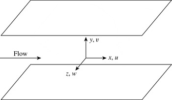
The flow configuration is shown in figure 1. Periodic boundary conditions are enforced in the streamwise,
 $x$
, and spanwise,
 $z$
, directions and no-slip conditions at both walls. The simulations are performed at a Reynolds number
 $\mathit{Re}=2000$
based on the channel half-height,
 $h$
, and the bulk flow velocity,
 $U_{b}$
. The Weissenberg number is therefore
 $\mathit{We}\equiv {\it\lambda}U_{b}/h$
, where
 ${\it\lambda}$
is the polymer relaxation time. Throughout this work, time,
 $t$
, is normalized by the convective time scale,
 $h/U_{b}$
, but can readily be expressed in reference to the relaxation time scale,
 $t_{{\it\lambda}}=t/\mathit{We}$
.
Flow configuration and coordinate system.

The mass flow rate is maintained constant by adjusting the required streamwise pressure gradient. Since the focus is on bypass transition, the Reynolds number is lower than the critical value for Newtonian channel flow,
 $\mathit{Re}_{c}=3848$
(Orszag Reference Orszag1971), and non-Newtonian flow at similar rheological conditions,
 $\mathit{Re}_{c}=3600$
for a FENE-P fluid at
 ${\it\beta}=0.9$
and high maximum extensibility (see figure 5 in Zhang et al.
Reference Zhang, Lashgari, Zaki and Brandt2013).
The initial condition for the simulations consists of a laminar base state, along with a localized velocity perturbation. The laminar base state for non-Newtonian flow, as reported by Richter, Iaccarino & Shaqfeh (Reference Richter, Iaccarino and Shaqfeh2010), is given by
 $$\begin{eqnarray}\displaystyle & & \displaystyle U(y)=\frac{\mathit{Re}}{2{\it\beta}}\frac{\text{d}P}{\text{d}x}(y^{2}-1)-\frac{1-{\it\beta}}{{\it\beta}}\frac{3}{8J_{0}}\left[(F^{+}(y)G^{-}(y)+F^{-}(y)G^{+}(y))\right.\nonumber\\ \displaystyle & & \displaystyle \left.\qquad \quad -\,(F^{+}(h)G^{-}(h)+F^{-}(h)G^{+}(h))\right]\end{eqnarray}$$
 $$\begin{eqnarray}\displaystyle & \displaystyle F^{\pm }(y)=\left(J_{0}y\pm \sqrt{(J_{0}y)^{2}+K_{0}^{3}}\right)^{1/3} & \displaystyle\end{eqnarray}$$
 $$\begin{eqnarray}\displaystyle & \displaystyle G^{\pm }(y)=\left(3J_{0}y\pm \sqrt{(J_{0}y)^{2}+K_{0}^{3}}\right)^{1/3} & \displaystyle\end{eqnarray}$$
 $$\begin{eqnarray}\displaystyle & \displaystyle J_{0}=\frac{\mathit{Re}}{4{\it\beta}}\left(\frac{L_{max}}{a\mathit{We}}\right)^{2}\frac{\text{d}P}{\text{d}x} & \displaystyle\end{eqnarray}$$
 $$\begin{eqnarray}\displaystyle & \displaystyle K_{0}=\frac{1}{6{\it\beta}}\left(\frac{L_{max}}{a\mathit{We}}\right)^{2}. & \displaystyle\end{eqnarray}$$
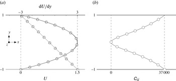
The difference between the velocity profiles for Poiseuille (
 ${\it\beta}=1$
in (2.7)) and non-Newtonian laminar flow is negligible for the values of
 $\mathit{We}$
and
 ${\it\beta}$
used here as demonstrated by the comparison in figure 2. The trace of the associated polymeric conformation tensor is also shown.
Mean velocity profile, mean shear, and trace of the conformation tensor at
 $t=0$
for
 $\mathit{Re}=2000$
:
 $\boldsymbol{\cdot }\boldsymbol{\cdot }\boldsymbol{\cdot }\,\boldsymbol{\cdot }$
,
 $\text{d}U/\text{d}y$
; ▵, Newtonian flow; ○, non-Newtonian flow at
 $\mathit{We}=100$
,
 $L_{max}=300$
and
 ${\it\beta}=0.9$
.

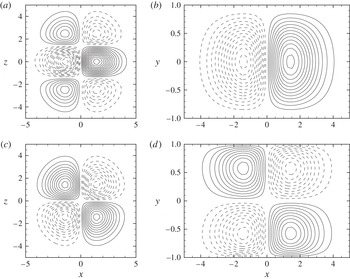
The localized disturbance added to the base flow is a pair of counter-rotating vortices (figure 3), previously used by Henningson et al. (Reference Henningson, Lundbladh and Johansson1993) in simulations of Newtonian channel flow. The disturbance is placed at the centre of the channel and spans the entire channel height. The streamwise and spanwise extents, and the disturbance orientation and amplitude can be specified. The disturbance streamfunction and velocity are
 $$\begin{eqnarray}\displaystyle & \displaystyle {\it\psi}={\it\epsilon}f(y)\left(\frac{x^{\prime }}{l_{x}}\right)z^{\prime }\exp \left[-\!\left(\frac{x^{\prime }}{l_{x}}\right)^{2}-\!\left(\frac{z^{\prime }}{l_{z}}\right)^{2}\right] & \displaystyle\end{eqnarray}$$
 $$\begin{eqnarray}\displaystyle & \displaystyle (u^{\prime },v^{\prime },w^{\prime })=\left(-\frac{\partial {\it\psi}}{\partial y}\sin {\it\theta},\frac{\partial {\it\psi}}{\partial z^{\prime }},-\frac{\partial {\it\psi}}{\partial y}\cos {\it\theta}\right) & \displaystyle\end{eqnarray}$$
 $$\begin{eqnarray}\displaystyle & (x^{\prime },z^{\prime })=(x\cos {\it\theta}-z\sin {\it\theta},x\sin {\it\theta}+z\cos {\it\theta}) & \displaystyle\end{eqnarray}$$
 $$\begin{eqnarray}\displaystyle & f(y)=(1+y)^{p}(1-y)^{q}. & \displaystyle\end{eqnarray}$$
 $l_{x}$
,
 $l_{y}$
and
 $l_{z}$
are the streamwise, wall-normal and spanwise length scales of the disturbance and
 ${\it\epsilon}$
is its amplitude. For this study,
 $l_{x}=l_{z}=2$
. The exponents of the wall-normal dependence are also equal,
 $p=q=2$
. The orientation of the disturbance in the horizontal plane is dependent on
 ${\it\theta}$
; for the current study,
 ${\it\theta}=0$
.
Initial wall-normal and spanwise velocity perturbation fields: (a)
 $v^{\prime }$
at
 $y=-0.56$
, contour spacing
 $2.0\times 10^{-6}$
; (b)
 $v^{\prime }$
at
 $z=-1.0$
, contour spacing
 $2.0\times 10^{-6}$
; (c)
 $w^{\prime }$
at
 $y=-0.56$
, contour spacing
 $8.0\times 10^{-6}$
; (d)
 $w^{\prime }$
at
 $z=-1.0$
, contour spacing
 $8.0\times 10^{-6}$
. Solid and dashed lines indicate positive and negative velocities, respectively.

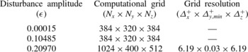
Details of the parameters of the computational domain are provided in table 1. The dimensions are in accordance with the recommendation by Li, Sureshkumar & Khomami (Reference Li, Sureshkumar and Khomami2006) for fully turbulent non-Newtonian flow. The grid spacing is uniform in the streamwise and spanwise directions and is given by a hyperbolic tangent stretching in the wall-normal coordinate. A grid refinement study was performed in order to ensure that the flow in the Newtonian and non-Newtonian cases is fully resolved.
In the following, instantaneous flow variables are decomposed according to
 ${\it\phi}(\boldsymbol{x},t)=\overline{{\it\phi}}(y,t)+{\it\phi}^{\prime }(\boldsymbol{x},t)$
. Overline and uppercase denote variables that are averaged in both the streamwise and spanwise directions, and
 ${\it\phi}^{\prime }(\boldsymbol{x},t)$
is the perturbation. Where integral quantities are plotted, they are averaged over the bottom half of the channel and are defined as,
 $\widehat{{\it\phi}}(t)\equiv 1/(L_{y}/2)\int _{-L_{y}/2}^{0}\overline{{\it\phi}}(y,t)\text{d}y$
. The difference between the non-Newtonian and Newtonian (
 $\widehat{{\it\phi}}_{N}(t)$
) values of a quantity is denoted by
 $[\widehat{{\it\phi}}](t)=\widehat{{\it\phi}}(t)-\widehat{{\it\phi}}_{N}(t)$
.
3. Evolution of linear disturbance
The study of transition is often aided by considering the evolution of small-amplitude, or linear, perturbations. In order to examine linear effects, a vortex pair with an amplitude
 ${\it\epsilon}=1.5\times 10^{-4}$
is prescribed as the initial disturbance. In the Orr–Sommerfeld and Squire equations for the wall-normal velocity and vorticity, the three-dimensionality of the initial disturbance, namely
 $\partial v^{\prime }/\partial z$
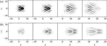
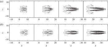
, causes forcing of the wall-normal vorticity perturbation. This results in an increase in the streamwise velocity perturbation and therefore energy growth owing to the linear lift-up mechanism (figure 4). This growth is opposed and eventually damped by viscous dissipation. Snapshots of the disturbance in Newtonian flow (figure 4) show the effect of dissipation: a decrease in the magnitude of perturbation velocities is observed at large times during the disturbance evolution. In figure 5, the evolution of the disturbance energy per unit volume,
 $E(t)$
, is plotted and is normalized by its initial value
 $E_{0}$
,
 $$\begin{eqnarray}E(t)\equiv \frac{1}{L_{x}\times L_{z}\times L_{y}/2}\int _{-L_{y}/2}^{0}\int _{-L_{z}/2}^{L_{z}/2}\int _{-L_{x}/2}^{L_{x}/2}\frac{1}{2}(u^{\prime 2}+v^{\prime 2}+w^{\prime 2})\text{d}x\text{d}z\text{d}y.\end{eqnarray}$$
Evolution of the disturbance (
 ${\it\epsilon}=1.5\times 10^{-4}$
) in Newtonian flow at
 $y=-0.56$
and
 $t=\{3,7,13,20\}$
. Contours denote (a) wall-normal
 $v^{\prime }$
and (b) streamwise
 $u^{\prime }$
velocity perturbations.

Parameters describing the computational domain and grid. The computational domain for all simulations presented has dimensions
 $L_{x}=48$
,
 $L_{y}=2$
,
 $L_{z}=24$
. The grid resolution is normalized by the wall variable
 $y^{+}=yu_{{\it\tau}}/{\it\nu}$
where
 ${\it\nu}$
is the kinematic viscosity and
 $u_{{\it\tau}}$
the friction velocity in the fully turbulent Newtonian flow.

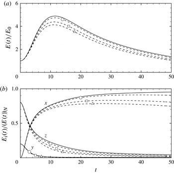
Evolution of perturbation energy for
 ${\it\epsilon}=1.5\times 10^{-4}$
. (a) Amplification of total perturbation energy normalized by the initial value. (b) Components of perturbation energy,
 $E_{i}(t)$
, normalized by the total energy in the Newtonian flow,
 $(E(t))_{N}$
. ——, Newtonian flow; - - - -, non-Newtonian flow at
 $L_{max}=300$
and
 ${\it\beta}=0.9$
; ○,
 $\mathit{We}=15$
; ▫,
 $\mathit{We}=40$
; ▵,
 $\mathit{We}=100$
.

The same trend of energy growth and decay in Newtonian flow is followed in the non-Newtonian case (figure 5
a), but the extent of energy amplification decreases. For the non-Newtonian cases shown, the energy suppression varies from approximately 5 to 15 %, depending on the elasticity of the flow. A decomposition of the perturbation energy in the three coordinate directions is shown in figure 5(b). The wall-normal and spanwise energy make up a progressively smaller fraction of the total energy with time. The streamwise energy, on the other hand, becomes dominant for
 $t>3.28$
. Its amplification and further decay therefore dictate the shape of the
 $E(t)$
curve in figure 5(a). Relative to the Newtonian case, viscoelasticity causes a faster decay in the spanwise energy and suppresses the streamwise energy growth. During the initial phase of energy amplification, these two components are comparable in magnitude. The wall-normal component is also suppressed, although inappreciably.
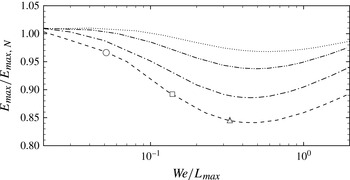
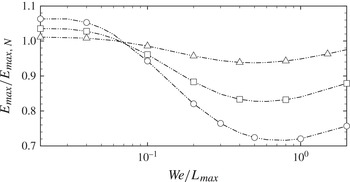
We now examine the influence of the ratio
 $\mathit{We}/L_{max}$
on
 $E_{max}\equiv \max _{t}\{E(t)\}$
, shown in figure 6, where the maximum perturbation kinetic energy is normalized by the Newtonian value,
 $E_{max,N}$
. For low
 $\mathit{We}/L_{max}$
, viscoelasticity appears to enhance transient growth, although inappreciably. The main region of interest here is for higher
 $\mathit{We}/L_{max}$
, where a significant decrease in the maximum perturbation energy is observed. This trend is consistent with the optimal disturbance results by Zhang et al. (Reference Zhang, Lashgari, Zaki and Brandt2013). Those authors reported a stabilizing effect of oblique disturbances at high We. The origin of the stabilizing influence observed in figure 6 is analysed in the next section by examining the perturbation-energy equation. The case with
 $\mathit{We}=40$
and
 $L_{max}=300$
is examined in detail since this relatively high Weissenberg number emphasizes the difference between the Newtonian and non-Newtonian flow. The change in trend at
 $\mathit{We}/L_{max}\sim 0.5$
is explained in § 3.2.
The effect of elasticity on the maximum perturbation energy in non-Newtonian flow:
 $\boldsymbol{\cdot }\boldsymbol{\cdot }\boldsymbol{\cdot }\,\boldsymbol{\cdot }$
,
 $L_{max}=50$
; — ⋅ ⋅ —,
 $L_{max}=100$
; — ⋅ —,
 $L_{max}=200$
; - - - -,
 $L_{max}=300$
; ○,
 $\mathit{We}=15$
; ▫,
 $\mathit{We}=40$
; ▵,
 $\mathit{We}=100$
.

An energy analysis was also performed by Hoda et al. (Reference Hoda, Jovanovic and Kumar2009) for a non-Newtonian channel flow perturbed with stochastic body forcing. In order to isolate the mechanism for streak formation and amplification, they focused on streamwise-independent linear disturbances. In contrast, the localized disturbance in the current study has a finite streamwise and spanwise extent, and the associated terms play an important role in the energy evolution.
3.1. Energy analysis
For the non-Newtonian polymeric flow, the transport equation for the Reynolds stress is given by
 $$\begin{eqnarray}\displaystyle \frac{\partial \overline{u_{i}^{\prime }u_{j}^{\prime }}}{\partial t} & = & \displaystyle \underbrace{-U_{k}\frac{\partial \overline{u_{i}^{\prime }u_{j}^{\prime }}}{\partial x_{k}}}_{\mathscr{A}_{ij}}\underbrace{-\frac{\partial \overline{u_{i}^{\prime }u_{j}^{\prime }u_{k}^{\prime }}}{\partial x_{k}}}_{\mathscr{Q}_{ij}}\underbrace{-\left(\overline{u_{j}^{\prime }\frac{\partial p^{\prime }}{\partial x_{i}}}+\overline{u_{i}^{\prime }\frac{\partial p^{\prime }}{\partial x_{j}}}\right)}_{{\it\phi}_{ij}}\nonumber\\ \displaystyle & & \displaystyle \underbrace{-\left(\overline{u_{j}^{\prime }u_{k}^{\prime }}\frac{\partial U_{i}}{\partial x_{k}}+\overline{u_{i}^{\prime }u_{k}^{\prime }}\frac{\partial U_{j}}{\partial x_{k}}\right)}_{\mathscr{P}_{ij}}+\underbrace{\frac{{\it\beta}}{\mathit{Re}}\frac{\partial ^{2}\overline{u_{i}^{\prime }u_{j}^{\prime }}}{\partial x_{k}^{2}}}_{\mathscr{D}_{ij}}\nonumber\\ \displaystyle & & \displaystyle \underbrace{-2\frac{{\it\beta}}{\mathit{Re}}\overline{\frac{\partial u_{i}^{\prime }}{\partial x_{k}}\frac{\partial u_{j}^{\prime }}{\partial x_{k}}}}_{{\it\epsilon}_{ij}}+\underbrace{\frac{1-{\it\beta}}{\mathit{Re}}\left(\overline{u_{j}^{\prime }\frac{\partial {\it\tau}_{ik}^{\prime }}{\partial x_{k}}}+\overline{u_{i}^{\prime }\frac{\partial {\it\tau}_{jk}^{\prime }}{\partial x_{k}}}\right)}_{\mathscr{W}_{ij}}.\end{eqnarray}$$
 $i=j$
,
 $$\begin{eqnarray}\frac{1}{2}\frac{\partial \widehat{u_{i}^{\prime }u_{i}^{\prime }}}{\partial t}=\frac{\partial E}{\partial t}=\frac{1}{2}(\widehat{\mathscr{A}}_{ii}+\widehat{\mathscr{Q}}_{ii}+\widehat{{\it\phi}}_{ii}+\widehat{\mathscr{P}}_{ii}+\widehat{\mathscr{D}}_{ii}+\widehat{{\it\epsilon}}_{ii}+\widehat{\mathscr{W}}_{ii}).\end{eqnarray}$$
In the above equation, repeating indices imply summation over the three coordinate directions. In (3.2),
 $\mathscr{A}_{ij}$
is mean advection,
 $\mathscr{Q}_{ij}$
is energy transport by fluctuations,
 ${\it\phi}_{ij}$
is pressure redistribution,
 $\mathscr{P}_{ij}$
is production,
 $\mathscr{D}_{ij}$
is viscous diffusion,
 ${\it\epsilon}_{ij}$
is dissipation and
 $\mathscr{W}_{ij}$
is polymer work. The polymer work,
 $\mathscr{W}_{ij}$
, depends on the perturbation to the polymer stress. The latter is governed by the evolution equation for the perturbation to the conformation tensor,
 $$\begin{eqnarray}\displaystyle \left(\frac{\partial }{\partial t}+U_{k}\frac{\partial }{\partial x_{k}}\right)\unicode[STIX]{x1D624}_{ij}^{\prime } & = & \displaystyle -u_{k}^{\prime }\frac{\partial \unicode[STIX]{x1D60A}_{ij}}{\partial x_{k}}-u_{k}^{\prime }\frac{\partial \unicode[STIX]{x1D624}_{ij}^{\prime }}{\partial x_{k}}+\unicode[STIX]{x1D60A}_{kj}\frac{\partial u_{i}^{\prime }}{\partial x_{k}}+\unicode[STIX]{x1D624}_{kj}^{\prime }\frac{\partial U_{i}}{\partial x_{k}}+\unicode[STIX]{x1D624}_{kj}^{\prime }\frac{\partial u_{i}^{\prime }}{\partial x_{k}}+\unicode[STIX]{x1D60A}_{ik}\frac{\partial u_{j}^{\prime }}{\partial x_{k}}\nonumber\\ \displaystyle & & \displaystyle +\,\unicode[STIX]{x1D624}_{ik}^{\prime }\frac{\partial U_{j}}{\partial x_{k}}+\unicode[STIX]{x1D624}_{ik}^{\prime }\frac{\partial u_{j}^{\prime }}{\partial x_{k}}-{\it\tau}_{ij}^{\prime }.\end{eqnarray}$$
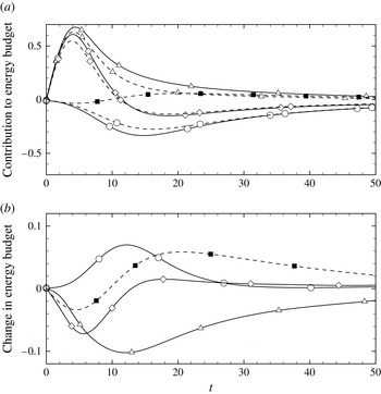
Components of the perturbation energy budget (see (3.3)): (a) ——, Newtonian flow; - - - -, non-Newtonian flow at
 $L_{max}=300$
,
 ${\it\beta}=0.9$
,
 $\mathit{We}=40$
; ▵,
 $\widehat{\mathscr{P}}_{ii}/2E_{0}$
; ○,
 $\widehat{{\it\epsilon}}_{ii}/2E_{0}$
; ▪,
 $\widehat{\mathscr{W}}_{ii}/2E_{0}$
; ⬥,
 $(1/2E_{0})\partial \widehat{u_{i}^{\prime }u_{i}^{\prime }}/\partial t$
; (b) ▵, [
 $\widehat{\mathscr{P}}_{ii}/2E_{0}$
]; ○, [
 $\widehat{{\it\epsilon}}_{ii}/2E_{0}$
]; ▪,
 $\widehat{\mathscr{W}}_{ii}/2E_{0}$
; ⬥, [
 $(1/2E_{0})\partial \widehat{u_{i}^{\prime }u_{i}^{\prime }}/\partial t$
].

In the linear evolution, the production, dissipation and polymer work are the only significant contributors to the energy budget (3.3). These contributions are compared with the Newtonian reference simulation in figure 7(a) and the difference between the Newtonian and non-Newtonian simulations is plotted in figure 7(b). Relative to the Newtonian case, both the production and dissipation are reduced, and the difference between the energy growth rate in the non-Newtonian and Newtonian flows,
 $[\partial \widehat{u_{i}^{\prime }u_{i}^{\prime }}/\partial t]$
, is negative thus signalling weaker energy amplification in the polymeric flow. The maximum
 $[\partial \widehat{u_{i}^{\prime }u_{i}^{\prime }}/\partial t]$
is recorded near
 $t\sim 6$
and is primarily due to a negative polymer work and a decrease in production, both of which contribute to the weaker energy amplification in the flow. The decrease in production is in agreement with the observations of Dimitropoulos et al. (Reference Dimitropoulos, Sureshkumar and Beris1998) and Zhang et al. (Reference Zhang, Lashgari, Zaki and Brandt2013) and represents a weaker rate of energy transfer from the mean flow to velocity fluctuations. The negative polymer work indicates that energy from the velocity fluctuations is exerted as work onto the polymer chains, an assertion which is further examined below.
3.1.1. Polymer work
Since the initial disturbance is a streamwise vortex with the majority of the energy in the spanwise component (see figure 5
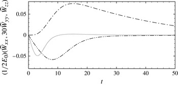
b), the polymer work term is expected to affect primarily the spanwise component of the velocity disturbance at early time. This view is supported by figure 8 where the time evolution of the polymer work is reported. The wall-normal polymer work is multiplied by a factor of 30 in the figure to emphasize that it is slightly negative. While this component is smaller than the dominant spanwise polymer work, it has an indirect effect on energy which will be analysed in the next section. Most relevant here, however, is the negative
 $\widehat{\mathscr{W}}_{zz}$
at early time,
 $$\begin{eqnarray}\displaystyle \mathscr{W}_{zz} & = & \displaystyle \frac{2(1-{\it\beta})}{\mathit{Re}}\left(\overline{w^{\prime }\frac{\partial {\it\tau}_{xz}^{\prime }}{\partial x}}+\overline{w^{\prime }\frac{\partial {\it\tau}_{yz}^{\prime }}{\partial y}}+\overline{w^{\prime }\frac{\partial {\it\tau}_{zz}^{\prime }}{\partial z}}\right)\nonumber\\ \displaystyle & = & \displaystyle \mathscr{W}_{zz(x)}+\mathscr{W}_{zz(y)}+\mathscr{W}_{zz(z)}.\end{eqnarray}$$
Evolution of the components of polymer work for
 $\mathit{We}=40$
,
 $L_{max}=300$
and
 ${\it\beta}=0.9$
;
— ⋅ —,
 $\widehat{\mathscr{W}}_{xx}/2E_{0}$
;
 $\boldsymbol{\cdot }\boldsymbol{\cdot }\boldsymbol{\cdot }\,\boldsymbol{\cdot }$
,
 $30\widehat{\mathscr{W}}_{yy}/2E_{0}$
; — ⋅ ⋅ —,
 $\widehat{\mathscr{W}}_{zz}/2E_{0}$
.

The relation between polymeric stress and conformation tensor is given by (2.3). An expression for the polymeric stress perturbation is derived by simplifying the equation using a Taylor series expansion and taking into account that
 $\unicode[STIX]{x1D60A}_{kk}+\unicode[STIX]{x1D624}_{kk}^{\prime }<L_{max}^{2}$
for the set of non-Newtonian parameters (
 $\mathit{We}\sim O(10)$
,
 $L_{max}\sim O(10^{2})$
) used in this study,
 $$\begin{eqnarray}{\it\tau}_{ij}^{\prime }\approx \frac{1}{\mathit{We}}\left(\frac{\unicode[STIX]{x1D60A}_{ij}\unicode[STIX]{x1D624}_{kk}^{\prime }}{L_{max}^{2}}+\unicode[STIX]{x1D624}_{ij}^{\prime }\left(1+\frac{\unicode[STIX]{x1D60A}_{kk}+\unicode[STIX]{x1D624}_{kk}^{\prime }}{L_{max}^{2}}\right)\right)\approx \left(1+\frac{\unicode[STIX]{x1D60A}_{kk}}{L_{max}^{2}}\right)\frac{\unicode[STIX]{x1D624}_{ij}^{\prime }}{\mathit{We}}.\end{eqnarray}$$
The final simplification in the equation above is valid for
 $\unicode[STIX]{x1D60A}_{ij}/L_{max}^{2}\ll 1$
. This holds for all components except
 $i=j=x$
since
 $\unicode[STIX]{x1D60A}_{xx}\sim O(\mathit{We}^{2})$
. In order to explain the origin of the spanwise polymer work, we consider the evolution of a small-amplitude perturbation to the conformation tensor governed by the linear approximation of the full transport equation for the conformation tensor perturbation (3.4),
 $$\begin{eqnarray}\displaystyle \left(\frac{\partial }{\partial t}+U_{k}\frac{\partial }{\partial x_{k}}\right)\unicode[STIX]{x1D624}_{ij}^{\prime }=-u_{k}^{\prime }\frac{\partial \unicode[STIX]{x1D60A}_{ij}}{\partial x_{k}}+\unicode[STIX]{x1D60A}_{kj}\frac{\partial u_{i}^{\prime }}{\partial x_{k}}+\unicode[STIX]{x1D624}_{kj}^{\prime }\frac{\partial U_{i}}{\partial x_{k}}+\,\unicode[STIX]{x1D60A}_{ik}\frac{\partial u_{j}^{\prime }}{\partial x_{k}}+\unicode[STIX]{x1D624}_{ik}^{\prime }\frac{\partial U_{j}}{\partial x_{k}}-{\it\tau}_{ij}^{\prime }. & & \displaystyle\end{eqnarray}$$
 $V=W=0$
and
 $\unicode[STIX]{x1D60A}_{xz}=\unicode[STIX]{x1D60A}_{yz}=0$
. Therefore, the conformation tensor perturbations obey the governing equations,
 $$\begin{eqnarray}\displaystyle \left(\frac{\partial }{\partial t}+U\frac{\partial }{\partial x}\right)\unicode[STIX]{x1D624}_{xz}^{\prime } & = & \displaystyle \unicode[STIX]{x1D60A}_{zz}\frac{\partial u^{\prime }}{\partial z}+\unicode[STIX]{x1D624}_{yz}^{\prime }\frac{\partial U}{\partial y}+\unicode[STIX]{x1D60A}_{xx}\frac{\partial w^{\prime }}{\partial x}+\unicode[STIX]{x1D60A}_{xy}\frac{\partial w^{\prime }}{\partial y}-{\it\tau}_{xz}^{\prime }\nonumber\\ \displaystyle & {\approx} & \displaystyle \underbrace{\frac{\partial w^{\prime }}{\partial x}\unicode[STIX]{x1D60A}_{xx}}_{O\left(\frac{w^{\prime }}{l_{x}}\mathit{We}^{2}\right)}\end{eqnarray}$$
 $$\begin{eqnarray}\displaystyle \left(\frac{\partial }{\partial t}+U\frac{\partial }{\partial x}\right)\unicode[STIX]{x1D624}_{yz}^{\prime } & = & \displaystyle \unicode[STIX]{x1D60A}_{zz}\frac{\partial v^{\prime }}{\partial z}+\unicode[STIX]{x1D60A}_{xy}\frac{\partial w^{\prime }}{\partial x}+\unicode[STIX]{x1D60A}_{yy}\frac{\partial w^{\prime }}{\partial y}-{\it\tau}_{yz}^{\prime }\nonumber\\ \displaystyle & {\approx} & \displaystyle \underbrace{\frac{\partial w^{\prime }}{\partial x}\unicode[STIX]{x1D60A}_{xy}}_{O\left(\frac{w^{\prime }}{l_{x}}\mathit{We}\right)}\end{eqnarray}$$
 $$\begin{eqnarray}\displaystyle \left(\frac{\partial }{\partial t}+U\frac{\partial }{\partial x}\right)\unicode[STIX]{x1D624}_{zz}^{\prime } & = & \displaystyle -v^{\prime }\frac{\partial \unicode[STIX]{x1D60A}_{zz}}{\partial y}+2\unicode[STIX]{x1D60A}_{zz}\frac{\partial w^{\prime }}{\partial z}-{\it\tau}_{zz}^{\prime }\nonumber\\ \displaystyle & {\approx} & \displaystyle -\underbrace{v^{\prime }\frac{\partial \unicode[STIX]{x1D60A}_{zz}}{\partial y}}_{O\left(\frac{v^{\prime }}{l_{y}}\right)}+\underbrace{2\unicode[STIX]{x1D60A}_{zz}\frac{\partial w^{\prime }}{\partial z}}_{O\left(\frac{w^{\prime }}{l_{z}}\right)}.\end{eqnarray}$$
The above approximations are valid at short time (
 $t<\mathit{We}$
) and take into account that
 $\unicode[STIX]{x1D60A}_{zz}\sim O(1)$
,
 $\unicode[STIX]{x1D60A}_{xy}\sim O(\mathit{We})$
and
 $\unicode[STIX]{x1D60A}_{xx}\sim O(\mathit{We}^{2})$
. Further, the extent of the disturbance in all three directions (
 $l_{x}$
,
 $l_{y}$
,
 $l_{z}$
) is comparable at the early time. From the above equations, it is evident that the perturbation
 $\unicode[STIX]{x1D624}_{xz}^{\prime }$
, and in turn
 ${\it\tau}_{xz}^{\prime }$
, are dominant contributors to the negative spanwise polymer work. The physical mechanism in the approximation (3.8) is the action of the initial wall-normal vorticity which tilts, or rotates, the mean
 $\unicode[STIX]{x1D60A}_{xx}$
component of the conformation tensor and thus creates a perturbation
 $\unicode[STIX]{x1D624}_{xz}^{\prime }$
. This will in turn result in the polymer stress perturbation
 ${\it\tau}_{xz}^{\prime }$
, and ultimately a negative polymer work term
 $\overline{w^{\prime }(\partial {\it\tau}_{xz}^{\prime }/\partial x)}$
in the
 $\overline{w^{\prime }w^{\prime }}$
equation. Therefore, the kinetic energy from the spanwise velocity perturbation field is diminished as it is expended to stretch the polymer chains in the
 $x$
–
 $z$
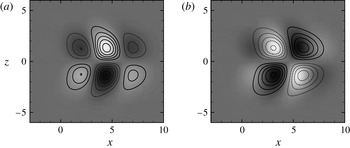
plane. Contour plots from the simulation at
 $t=4$
support this view: in figure 9(a),
 $\partial w^{\prime }/\partial x$
is in phase with
 $\unicode[STIX]{x1D624}_{xz}^{\prime }$
, consistent with the approximation (3.8). Furthermore, the resulting negative polymer work,
 $\mathscr{W}_{zz(x)}$
, is captured by the negative correlation between
 $w^{\prime }$
and
 $\partial {\it\tau}_{xz}^{\prime }/\partial x$
in figure 9(b). In summary, the wall-normal vorticity triggers a resistive spanwise polymer work which weakens the spanwise velocity of the localized disturbance as shown by the energy curves in figure 5(b).
Snapshots at
 $t=4$
,
 $y=-0.56$
during the evolution of the small-amplitude vortex pair in non-Newtonian flow at
 $\mathit{We}=40$
,
 $L_{max}=300$
and
 ${\it\beta}=0.9$
. (a) Contour lines,
 $\partial w^{\prime }/\partial x$
(contour spacing
 $2\times 10^{-5}$
); flood,
 $\unicode[STIX]{x1D624}_{xz}^{\prime }$
(contour range
 $[-3,3]$
). (b) Contour lines,
 $w^{\prime }$
(contour spacing
 $2\times 10^{-5}$
); flood,
 $\partial {\it\tau}_{xz}^{\prime }/\partial x$
(contour range
 $[-8\times 10^{-2},8\times 10^{-2}]$
).

3.1.2. Production of disturbance kinetic energy
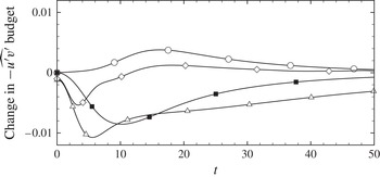
When considering the variation in the production term relative to Newtonian flow in figure 7, it is important to note that the change in the mean-velocity profile is negligible when the disturbance evolution is linear. Therefore the change in the averaged shear stress,
 $-\overline{u^{\prime }v^{\prime }}$
, is responsible for the decrease in production. The shear stress is, in turn, weaker due to a decrease in its own production term,
 $\overline{v^{\prime }v^{\prime }}(\partial U/\partial y)$
, during the initial energy growth phase (see figure 10).
Difference between the corresponding components of the shear stress budget in non-Newtonian and Newtonian flow: ▵,
 $[-\widehat{\mathscr{P}}_{xy}/2E_{0}]$
; ○,
 $[-\widehat{{\it\epsilon}}_{xy}/2E_{0}]$
; ▪,
 $-\widehat{\mathscr{W}}_{xy}/2E_{0}$
; ⬥,
 $[-(1/2E_{0})\partial \widehat{u^{\prime }v^{\prime }}/\partial t]$
.

The reduction in
 $\overline{v^{\prime }v^{\prime }}$
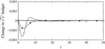
is examined by computing its budget (figure 11). The results demonstrate that the decrease in
 $\overline{v^{\prime }v^{\prime }}$
is mainly caused by a negative wall-normal polymer work,
 $$\begin{eqnarray}\displaystyle \mathscr{W}_{yy} & = & \displaystyle \frac{2(1-{\it\beta})}{\mathit{Re}}\left(\overline{v^{\prime }\frac{\partial {\it\tau}_{xy}^{\prime }}{\partial x}}+\overline{v^{\prime }\frac{\partial {\it\tau}_{yy}^{\prime }}{\partial y}}+\overline{v^{\prime }\frac{\partial {\it\tau}_{zy}^{\prime }}{\partial z}}\right)\nonumber\\ \displaystyle & = & \displaystyle \mathscr{W}_{yy(x)}+\mathscr{W}_{yy(y)}+\mathscr{W}_{yy(z)}.\end{eqnarray}$$
Difference between the corresponding components of
 $\partial \overline{v^{\prime 2}}/\partial t$
(see (3.2)) in non-Newtonian and Newtonian flow: ▵,
 $[\widehat{\mathscr{P}}_{yy}/2E_{0}]$
; ○,
 $[\widehat{{\it\epsilon}}_{yy}/2E_{0}]$
; ▪,
 $\widehat{\mathscr{W}}_{yy}/2E_{0}$
; ⬥,
 $[(1/2E_{0})\partial \widehat{v^{\prime }v^{\prime }}/\partial t]$
.

The origin of this component of the polymer work can be explained in a manner similar to that for the negative spanwise polymer work. Taking into account the simplification for the polymeric stress perturbation in (3.6) and the base state (
 $V=W=0$
and
 $\unicode[STIX]{x1D60A}_{xz}=\unicode[STIX]{x1D60A}_{yz}=0$
), the evolution of the relevant conformation tensor perturbations is determined from (3.7),
 $$\begin{eqnarray}\displaystyle \left(\frac{\partial }{\partial t}+U\frac{\partial }{\partial x}\right)\unicode[STIX]{x1D624}_{xy}^{\prime } & = & \displaystyle -v^{\prime }\frac{\partial \unicode[STIX]{x1D60A}_{xy}}{\partial y}+\unicode[STIX]{x1D60A}_{xy}\frac{\partial u^{\prime }}{\partial x}+\unicode[STIX]{x1D60A}_{yy}\frac{\partial u^{\prime }}{\partial y}+\unicode[STIX]{x1D624}_{yy}^{\prime }\frac{\partial U}{\partial y}\nonumber\\ \displaystyle & & \displaystyle +\,\unicode[STIX]{x1D60A}_{xx}\frac{\partial v^{\prime }}{\partial x}+\unicode[STIX]{x1D60A}_{xy}\frac{\partial v^{\prime }}{\partial y}-{\it\tau}_{xy}^{\prime }\nonumber\\ \displaystyle & {\approx} & \displaystyle \underbrace{\frac{\partial v^{\prime }}{\partial x}\unicode[STIX]{x1D60A}_{xx}}_{O\left(\frac{v^{\prime }}{l_{x}}\mathit{We}^{2}\right)}\end{eqnarray}$$
 $$\begin{eqnarray}\displaystyle \left(\frac{\partial }{\partial t}+U\frac{\partial }{\partial x}\right)\unicode[STIX]{x1D624}_{yy}^{\prime } & = & \displaystyle -v^{\prime }\frac{\partial \unicode[STIX]{x1D60A}_{yy}}{\partial y}+2\left(\unicode[STIX]{x1D60A}_{xy}\frac{\partial v^{\prime }}{\partial x}+\unicode[STIX]{x1D60A}_{yy}\frac{\partial v^{\prime }}{\partial y}\right)-{\it\tau}_{yy}^{\prime }\nonumber\\ \displaystyle & {\approx} & \displaystyle \underbrace{2\frac{\partial v^{\prime }}{\partial x}\unicode[STIX]{x1D60A}_{xy}}_{O\left(\frac{v^{\prime }}{l_{x}}\mathit{We}\right)}\end{eqnarray}$$
 $$\begin{eqnarray}\displaystyle \left(\frac{\partial }{\partial t}+U\frac{\partial }{\partial x}\right)\unicode[STIX]{x1D624}_{yz}^{\prime } & = & \displaystyle \unicode[STIX]{x1D60A}_{zz}\frac{\partial v^{\prime }}{\partial z}+\unicode[STIX]{x1D60A}_{xy}\frac{\partial w^{\prime }}{\partial x}+\unicode[STIX]{x1D60A}_{yy}\frac{\partial w^{\prime }}{\partial y}-{\it\tau}_{yz}^{\prime }\nonumber\\ \displaystyle & {\approx} & \displaystyle \underbrace{\frac{\partial w^{\prime }}{\partial x}\unicode[STIX]{x1D60A}_{xy}}_{O\left(\frac{w^{\prime }}{l_{x}}\mathit{We}\right)}.\end{eqnarray}$$
As for the spanwise polymer work, the approximations above are valid for early time and utilize the relations,
 $\unicode[STIX]{x1D60A}_{xy}\sim O(\mathit{We})$
and
 $\unicode[STIX]{x1D60A}_{xx}\sim O(\mathit{We}^{2})$
. Comparing the simplified equations,
 $\unicode[STIX]{x1D624}_{xy}^{\prime }$
is the dominant contributor to the wall-normal polymer work. The approximation (3.12) is the action of the spanwise vorticity perturbation
 $\partial v^{\prime }/\partial x$
which tilts, or rotates, the mean conformation tensor
 $\unicode[STIX]{x1D60A}_{xx}$
, and thus amplifies
 $\unicode[STIX]{x1D624}_{xy}^{\prime }$
. This is captured in figure 12(a) where contours of
 $\partial v^{\prime }/\partial x$
coincide with
 $\unicode[STIX]{x1D624}_{xy}^{\prime }$
. The resulting perturbation in the polymer stress is
 ${\it\tau}_{xy}^{\prime }$
, and the associated polymer work
 $\mathscr{W}_{yy(x)}$
is negative as demonstrated by the negative correlation between
 $v^{\prime }$
and
 $\partial {\it\tau}_{xy}^{\prime }/\partial x$
in figure 12(b). This polymer work term therefore extracts energy from
 $\overline{v^{\prime }v^{\prime }}$
. The impact is important because a weaker
 $\overline{v^{\prime }v^{\prime }}$
leads to a decrease in the production of the Reynolds shear stress
 $\overline{u^{\prime }v^{\prime }}$
and, in turn, in the production of
 $\overline{u^{\prime }u^{\prime }}$
which is the principal contributor to energy amplification.
Snapshots at
 $t=4$
,
 $y=-0.56$
during the evolution of the small-amplitude vortex pair in non-Newtonian flow at
 $\mathit{We}=40$
,
 $L_{max}=300$
and
 ${\it\beta}=0.9$
. (a) Contour lines,
 $\partial v^{\prime }/\partial x$
(contour spacing
 $5\times 10^{-6}$
); flood,
 $\unicode[STIX]{x1D624}_{xy}^{\prime }$
(contour range
 $[-0.6,0.6]$
). (b) Contour lines,
 $v^{\prime }$
(contour spacing
 $5\times 10^{-6}$
); flood,
 $\partial {\it\tau}_{xy}^{\prime }/\partial x$
(contour range
 $[-2\times 10^{-2},2\times 10^{-2}]$
).

The two terms
 $\mathscr{W}_{zz(x)}$
and
 $\mathscr{W}_{yy(x)}$
are dominant because they are associated with perturbations to the mean streamwise polymer stress. In the limit of streamwise-independent disturbances, however, both terms vanish and, as a result, they were not part of the energy analysis by Hoda et al. (Reference Hoda, Jovanovic and Kumar2009). In that work, the streamwise polymer-work term makes the leading contribution, and acts to increase the energy amplification which is consistent with the sign of
 $W_{xx}$
in the current simulations (see figure 8).
In summary, the polymer work plays a dual role in reducing the disturbance energy in the current flow configuration, with both effects acting on the streamwise vortex: first, a direct effect is due to the negative spanwise polymer work
 $\widehat{\mathscr{W}}_{zz}$
on
 $\overline{w^{\prime }w^{\prime }}$
. Second, an indirect effect is via the wall-normal
 $\widehat{\mathscr{W}}_{yy}$
term which suppresses
 $\overline{v^{\prime }v^{\prime }}$
and, as a result, the production of
 $\overline{u^{\prime }v^{\prime }}$
and ultimately of the disturbance kinetic energy.
3.2. Influence of elasticity beyond
 $\mathit{We}/L_{max}\sim 0.5$

The stabilizing influence of the polymer in terms of suppressing energy amplification was discussed above. Figure 6, however, also shows that this effect is reduced for
 $\mathit{We}/L_{max}>0.5$
. This is a result of the nonlinear dependence of the polymer stress on the polymer conformation for the FENE-P model and is illustrated below.
In the previous section, energy suppression was explained in terms of the perturbations to the conformation tensor,
 $\unicode[STIX]{x1D624}_{xz}^{\prime }$
and
 $\unicode[STIX]{x1D624}_{xy}^{\prime }$
, which arise due to the vorticity perturbation acting on the mean conformation. The elastic effect of the polymer is fed back to the velocity field through the polymer stress. Using the simplification (3.6) for the polymeric stress perturbation, the evolution of
 ${\it\tau}_{xz}^{\prime }$
is governed by,
 $$\begin{eqnarray}\left(\frac{\partial }{\partial t}+U\frac{\partial }{\partial x}\right){\it\tau}_{xz}^{\prime }\approx \frac{\partial w^{\prime }}{\partial x}\frac{\unicode[STIX]{x1D60A}_{xx}}{\mathit{We}}\left(1+\frac{\unicode[STIX]{x1D60A}_{kk}}{L_{max}^{2}}\right)\approx \frac{\partial w^{\prime }}{\partial x}\overline{{\it\tau}}_{xx}.\end{eqnarray}$$
A similar expression governs the early time behaviour of
 ${\it\tau}_{xy}^{\prime }$
,
 $$\begin{eqnarray}\left(\frac{\partial }{\partial t}+U\frac{\partial }{\partial x}\right){\it\tau}_{xy}^{\prime }\approx \frac{\partial v^{\prime }}{\partial x}\overline{{\it\tau}}_{xx}.\end{eqnarray}$$
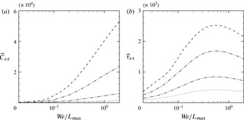
The perturbation stress therefore arises due to the action of the vorticity disturbance onto the mean stress, in analogy to the conformation. Figure 13 shows the dependence of
 $\widehat{\unicode[STIX]{x1D60A}}_{xx}$
and
 $\widehat{{\it\tau}}_{xx}$
on
 $\mathit{We}/L_{max}$
. While the mean conformation tensor increases monotonically with increasing
 $\mathit{We}/L_{max}$
, the mean stress tensor reaches a maxima at
 $\mathit{We}/L_{max}\sim 0.5$
. In a sense, the reservoir of mean stress from which the perturbation stress, and consequently polymer work, are extracted diminishes (similar behaviour was observed in mixing layers by Ray & Zaki Reference Ray and Zaki2014). Beyond the maxima,
 $\widehat{{\it\tau}}_{xx}$
decreases and as a result the perturbations
 ${\it\tau}_{xz}^{\prime }$
and
 ${\it\tau}_{xy}^{\prime }$
also decrease, which weakens the polymer work, or the influence of elasticity.
Variation of ‘
 $xx$
’ component of the mean conformation tensor and polymeric stress tensor:
 $\boldsymbol{\cdot }\boldsymbol{\cdot }\boldsymbol{\cdot }\,\boldsymbol{\cdot }$
,
 $L_{max}=50$
; — ⋅ ⋅ —,
 $L_{max}=100$
; — ⋅ —,
 $L_{max}=200$
; - - - -,
 $L_{max}=300$
.

3.3. Effect of increasing polymer concentration
For all of the results reported so far, a solution with low polymer concentration has been considered,
 ${\it\beta}=0.9$
. In a solution with higher polymer concentration, or a lower
 ${\it\beta}$
, the effects of the polymer are expected to be enhanced, and the results indicate that this is indeed the case as shown in figure 14.
The effect of polymer concentration, represented by
 ${\it\beta}$
, on the maximum perturbation energy in non-Newtonian flow: ▵,
 ${\it\beta}=0.9$
; ▫,
 ${\it\beta}=0.7$
; ○,
 ${\it\beta}=0.5$
.

The energy analysis reveals that the mechanism for energy suppression remains unchanged, and that the enhanced effect of the polymer is primarily due to the corresponding increase in the magnitude of the polymer work, which was previously identified as the cause of the reduced energy amplification. This is illustrated in figure 15 where the magnitude of polymer work is shown to increase with polymer concentration.
The effect of
 ${\it\beta}$
on polymer work during the evolution of the small amplitude vortex pair at
 $\mathit{We}=30$
and
 $L_{max}=100$
: ▵,
 ${\it\beta}=0.9$
; ▫,
 ${\it\beta}=0.7$
; ○,
 ${\it\beta}=0.5$
.

4. Nonlinear evolution
A high-amplitude initial disturbance leads to a regime of nonlinear development beyond a short-lived initial linear phase. Results from the evolution of disturbances with amplitudes sufficiently large to cause nonlinear growth are presented by Henningson et al. (Reference Henningson, Lundbladh and Johansson1993) for the Newtonian flow (
 ${\it\epsilon}=0.10485$
for the moderate-amplitude disturbance and
 ${\it\epsilon}=0.2097$
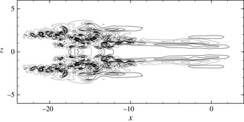
for the large-amplitude disturbance). The authors state that the nonlinear regime is characterized by pronounced streaky structures in the streamwise direction. Streak amplification can be understood in the linear growth limit by the lift-up mechanism (Landahl Reference Landahl1975). In the current flow configuration, the moderate- and large-amplitude localized disturbances generate, by nonlinear interactions, low-frequency components that lead to the emergence of more pronounced streaky structures via the lift-up mechanism (see figure 16). While the streaks decay in the case of the moderate amplitude disturbance, breakdown to turbulence is initiated in the case of the large-amplitude disturbance via a roll-up mechanism. As a result, a turbulent spot is formed (figure 17) and spreads thus leading to fully turbulent flow.
Evolution of the disturbance (
 ${\it\epsilon}=0.10485$
) in Newtonian flow at
 $y=-0.56$
and
 $t=\{7,13,20,27\}$
; (a) wall-normal
 $v^{\prime }$
and (b) streamwise
 $u^{\prime }$
velocity perturbations.

Turbulent spot in contours of
 $v^{\prime }$
at
 $t=40$
and
 $y=-0.56$
during the evolution of a large vortex pair (
 ${\it\epsilon}=0.2097$
) in Newtonian flow. Contour spacing
 $3.75\times 10^{-2}$
.

4.1. Evolution of the moderate amplitude vortex pair in non-Newtonian flow
The normalized energy amplification,
 $E(t)/E_{0}$
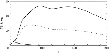
, in the case of a moderate-amplitude vortex pair is shown in figure 18. The three curves correspond to the linear and nonlinear evolutions of the Newtonian case, and the nonlinear energy growth of the polymeric flow. The parameters
 $\mathit{We}=15$
and
 $L_{max}=100$
were selected for the viscoelastic fluid since they are comparable to those used in previous studies of fully turbulent non-Newtonian channel flow (Dimitropoulos et al.
Reference Dimitropoulos, Sureshkumar and Beris1998; Dubief et al.
Reference Dubief, White, Terrapon, Shaqfeh, Moin and Lele2004; Dallas et al.
Reference Dallas, Vassilicos and Hewitt2010).
Evolution of energy amplification for
 ${\it\epsilon}=0.10485$
: ——, Newtonian flow; - - - -, non-Newtonian flow at
 $L_{max}=100$
,
 ${\it\beta}=0.9$
and
 $\mathit{We}=15$
; ▵,
 ${\it\epsilon}=0.00015$
.

At early times,
 $t\lesssim 10$
, the linear and nonlinear simulations are in agreement. Beyond
 $t=10$
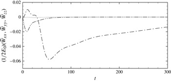
, the nonlinear energy growth departs from the curve for the linear evolution. For the non-Newtonian flow, there is a substantial reduction in the nonlinear growth phase. This phase is characterized by streaky structures with high streamwise perturbation velocity. The energy suppression suggests that these structures are weakened in the non-Newtonian case. The three components of polymer work are evaluated in figure 19. During the initial linear growth, the mechanism discussed for the evolution of the small amplitude vortex pair is applicable: namely the influence of negative spanwise and wall-normal polymer work.
Evolution of the components of polymer work for
 ${\it\epsilon}=0.10485$
,
 $\mathit{We}=15$
,
 $L_{max}=100$
and
 ${\it\beta}=0.9$
:
— ⋅ —,
 $\widehat{\mathscr{W}}_{xx}$
;
 $\boldsymbol{\cdot }\boldsymbol{\cdot }\boldsymbol{\cdot }\,\boldsymbol{\cdot }$
,
 $\widehat{\mathscr{W}}_{yy}$
; — ⋅ ⋅ —,
 $\widehat{\mathscr{W}}_{zz}$
.

Beyond
 $t=30$
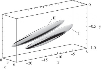
, a negative streamwise component of polymer work dominates and acts to oppose the growth of streaks (figure 19). A snapshot of the instantaneous negative polymer work and its correlation with the streaky structures in the flow at
 $t=40$
is shown in figure 20. In the figure, I and II are isosurfaces of the positive and negative streaks respectively, staggered in the spanwise direction such that II is closer to the central
 $x$
–
 $y$
plane of the channel. The isosurfaces are coloured with the negative streamwise polymer work that dominates during this nonlinear growth phase. There is a region of strong negative streamwise polymer work aligned along each streaky structure in the flow, illustrating a strong correlation between the streaky structures and
 $\mathscr{W}_{xx}<0$
. This correlation supports the hypothesis that the streamwise polymer work suppresses streaks during this early phase of nonlinear growth, consistent with the suppression in the perturbation energy. The weakening of streaks due to viscoelasticity has also been observed in the fully turbulent regime in previous studies (Dallas et al.
Reference Dallas, Vassilicos and Hewitt2010), especially at Weissenberg numbers which match those examined in the current simulations. With weaker streamwise streaks, transition to turbulence is expected to be prolonged in viscoelastic flow: a phenomenon which we examine next.
Isosurfaces of the streamwise perturbation velocity (I,
 $u^{\prime }=0.2$
; and II,
 $u^{\prime }=-0.2$
), coloured by the streamwise polymer work at
 $t=40$
. Contour levels range from
 $\mathscr{W}_{xx}/2E_{0}=-3.3$
(black) to
 $\mathscr{W}_{xx}/2E_{0}=-1.1$
(white).

4.2. Breakdown to turbulence in non-Newtonian flow
For the moderate-amplitude vortex pair case, the formation of streaks is followed by disturbance decay and the flow returns to a laminar state. A higher-amplitude initial disturbance (
 ${\it\epsilon}=0.2097$
) is required to cause breakdown to turbulence as reported by Henningson et al. (Reference Henningson, Lundbladh and Johansson1993) for Newtonian flow. In response, the disturbance evolution follows the same stages of growth described for the two lower-amplitude disturbances, but continues to amplify beyond the formation of streaks, and supports the formation of a turbulent spot.
Snapshots of
 $u^{\prime }$
and
 $v^{\prime }$
at
 $t=50$
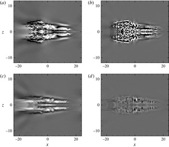
during the evolution of a large-amplitude vortex pair in Newtonian flow capture the shape of the spot (figure 21
a,b). At this time instance, the spot has returned to the centre of the domain due to the periodic boundary conditions. The spot can be divided into two parts: upstream of
 $x=0$
, the spot is composed primarily of small-scale structures; downstream of
 $x=0$
, the spot consists of large-scale structures oriented in the streamwise direction. The upstream region is more appreciably altered by the presence of the polymer in the non-Newtonian flow (figure 21
c,d), and the small-scale structures are visibly suppressed. The large-scale structures downstream of
 $x=0$
are still present, although at a lower magnitude. In Newtonian flow, the turbulent spot represents a region in which a statistically stationary turbulent state is approached (Henningson & Kim Reference Henningson and Kim1991). Adopting an analogous view in the non-Newtonian flow, and based on the observed changes to the turbulent spots, it is expected that the velocity perturbations in the eventual turbulent state will be significantly weaker. This prediction is in agreement with existing literature on fully turbulent non-Newtonian flow (e.g. Dubief et al.
Reference Dubief, White, Terrapon, Shaqfeh, Moin and Lele2004; Dallas et al.
Reference Dallas, Vassilicos and Hewitt2010).
Snapshots of perturbation velocity at
 $t=50$
and
 $y=-0.56$
during the evolution of the large-amplitude vortex pair. Newtonian flow: (a)
 $u^{\prime }=[-0.3,0.3]$
; (b)
 $v^{\prime }=[-0.05,0.05]$
. Non-Newtonian flow at
 $\mathit{We}=15$
,
 $L_{max}=100$
and
 ${\it\beta}=0.9$
: (c)
 $u^{\prime }$
; (d)
 $v^{\prime }$
with the same contour limits.

In Newtonian flow, the high-frequency region of the turbulent spot upstream of
 $x=0$
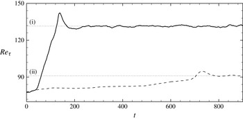
in figure 21 spreads and leads to fully turbulent flow in the entire channel. In the case of non-Newtonian flow, the perturbation velocity in that region is suppressed, and the late stages of the transition process whereby the turbulence spreads, fills the channel and becomes statistically stationary is substantially delayed. This delay is demonstrated in figures 22 and 23. In the former, the friction Reynolds number,
 $\mathit{Re}_{{\it\tau}}\equiv u_{{\it\tau}}h/{\it\nu}$
where
 $u_{{\it\tau}}$
is the friction velocity, is plotted as a function of time. The Newtonian curve rises from the initial laminar level to the turbulent state in a relatively short period of time. Beyond
 $t\sim 250$
, a fully turbulent state is maintained throughout the computational domain. The prolonged transition to turbulence in the non-Newtonian case is reflected in the longer time for
 $\mathit{Re}_{{\it\tau}}$
to level off,
 $t>800$
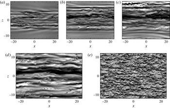
, even though its final level indicates a reduced-drag state. Snapshots of the polymeric flow during the transition process in figure 23 demonstrate the slow spreading of velocity perturbations across the channel. When a fully turbulent state is achieved, it differs significantly from that in Newtonian flow, as seen in figure 23(d,e), respectively.
Effect of the addition of polymers to the process of transition: ——, Newtonian; - - - -, non-Newtonian at
 $\mathit{We}=15$
,
 $L_{max}=100$
and
 ${\it\beta}=0.9$
. The dotted lines mark
 $\mathit{Re}_{{\it\tau}}$
in fully turbulent flow for the Newtonian (i) and non-Newtonian (ii) cases.

Snapshots of
 $u^{\prime }$
at
 $y=-0.56$
during the evolution of the large-amplitude vortex pair: (a–c) non-Newtonian flow during transition at
 $\mathit{We}=15$
,
 $L_{max}=100$
,
 ${\it\beta}=0.9$
and
 $t=\{200,400,600\}$
; (d) and (e) are a comparison of non-Newtonian and Newtonian flows, respectively, at
 $t=900$
. Contour limits:
 $[-0.2,0.2]$
.

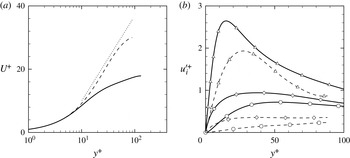
Ultimately the non-Newtonian flow reaches a drag-reduced turbulent state, close to the maximum drag reduction (MDR) state described by the Virk asymptote (Virk & Mickley Reference Virk and Mickley1970). Statistics from the turbulent regime,
 $t>800$
, are plotted in figure 24. The mean velocity profile for the non-Newtonian flow (figure 24
a) matches that of the Newtonian flow in the viscous sublayer. However, in the log layer, its slope is significantly increased. A drag reduction of 40 % is achieved in the current simulations. The r.m.s. velocity perturbations are compared to the Newtonian curves in figure 24(b). All three components of velocity have a weaker disturbance field in the polymeric flow. The recorded reduction in the r.m.s. is consistent with earlier work on drag-reduced flows (e.g. White & Mungal Reference White and Mungal2008). The statistics in figure 24 are also consistent with those in the elasto-inertial turbulence regime (Dubief, Terrapon & Soria Reference Dubief, Terrapon and Soria2013; Samanta et al.
Reference Samanta, Dubief, Holzner, Schafer and Morozov2013) where the authors report the formation of sheet-like structures of polymer extension which are large in the streamwise and spanwise dimensions. Structures with similar physical size are also established in the fully turbulent state of the current study. Since our computational domain is approximately five times larger in each of the horizontal directions, the structures are observed to occupy only a fraction of the channel width.
Statistics from fully turbulent flow: ——, Newtonian; - - - -, non-Newtonian at
 $\mathit{We}=15$
,
 $L_{max}=100$
and
 ${\it\beta}=0.9$
; (a) mean velocity profiles;
 $\boldsymbol{\cdot }\boldsymbol{\cdot }\boldsymbol{\cdot }\,\boldsymbol{\cdot }$
, Virk asymptote for MDR; (b) root-mean-squared velocity fluctuations; ▵, streamwise; ⬥, spanwise; ○, wall-normal.

The current simulations are performed at
 $\mathit{Re}=2000$
. Breakdown to turbulence in viscoelastic channel flow in the low-Reynolds-number regime where elastic forces are strong (Shaqfeh Reference Shaqfeh1996) is largely unexplored. Recent linear theory (Jovanovic & Kumar Reference Jovanovic and Kumar2011) and experiments (Pan et al.
Reference Pan, Morozov, Wagner and Arratia2013) demonstrate the potential for significant energy amplification and nonlinear subcritical instabilities in channel flow at
 $\mathit{Re}\ll 1$
. Future DNS of transition at low Reynolds number would complement these efforts.
5. Conclusion
This study is the first to detail the laminar-to-turbulence transition process in polymeric channel flow starting from a mathematically well-defined and reproducible disturbance. The numerical simulations capture the complete evolution of the disturbance until breakdown to turbulence. An energy analysis provides an explanation of the influence of polymer additives on the transition process which can be broadly divided into three phases. During the first linear phase, energy growth takes place via the lift-up mechanism. The wall-normal and spanwise vorticity perturbations tilt the mean conformation
 $\unicode[STIX]{x1D60A}_{xx}$
and generate
 $\unicode[STIX]{x1D624}_{xz}^{\prime }$
and
 $\unicode[STIX]{x1D624}_{xy}^{\prime }$
components. This results in negative polymer work which acts to suppress the spanwise and wall-normal components of perturbation velocity. Both effects lower the rate of energy growth in the linear stage, the former directly and the later indirectly by reducing the production of
 $\overline{u^{\prime }v^{\prime }}$
and in turn of
 $\overline{u^{\prime }u^{\prime }}$
. This is in agreement with the results for non-modal behaviour reported by Hoda et al. (Reference Hoda, Jovanovic and Kumar2008) and Zhang et al. (Reference Zhang, Lashgari, Zaki and Brandt2013). The lift-up mechanism results in the formation of streaky structures with high streamwise velocity perturbation, which are weakened by elasticity.
During the second phase, there is a significant growth of the streamwise streaks which reach high amplitude and nonlinear effects become important. During this stage, a negative streamwise polymer work weakens the streaky structures, causing a significant reduction in energy growth. The final step of transition is the formation of a turbulent spot, or breakdown to turbulence. The spot consists of a spectrum of flow structures: the streamwise-oriented structures from the preceding phase persist while small-scale structures are suppressed in the non-Newtonian flow. This leads to further suppression in the rate of energy growth and the transition process is prolonged. This delay in establishing turbulence motivates future studies of the influence of polymers on the secondary instability of the flow. The turbulent state which is established at long time is a drag-reduced state, close to the MDR asymptote.
The analysis of transition in the non-Newtonian flow has shed light on the effect of viscoelasticity on the linear and nonlinear stages. By focusing on an isolated initial disturbance, an uncluttered view of the transition process is possible and the disturbance evolution is examined in detail. The results from the late stages, or the nonlinear regime, naturally complement existing studies of viscoelastic turbulent channel flow.