


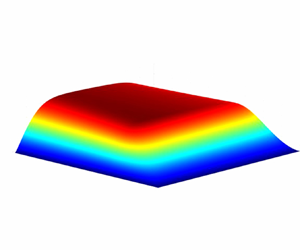

1. Introduction
The science of thin viscous films has been developed for a wide variety of applications including the lubrication of mechanical components, the spreading of droplets, coating processes, particle–particle interactions and biomechanics. It is well known that the flow dynamics in such films is governed by the Reynolds equation which, in its simplest form, is written as
 \begin{equation} \frac{{\rm d}}{{\rm d}\kern0.06em x}\left(h^{3}\frac{{\rm d}p}{{\rm d}\kern0.06em x} \right) =6\mu U \frac{{\rm d}h}{{\rm d}\kern0.06em x}, \end{equation}
where  $x$ is the spatial variable in the main flow direction,
 $h = h(x)$ is the film thickness,
 $p = p(x)$ is the fluid pressure,
 $\mu > 0$ is the constant shear viscosity and
 $U$ is a measure of fluid velocity in the main flow direction. Since first introduced by Osborne Reynolds (Reference Reynolds1886), equation (1.1) has formed the foundation of lubrication theory. To date, many scientists and engineers have extended (1.1) to include the effects of three dimensionality, non-Newtonian fluids, unsteadiness, turbulence, phase changes and more complex configurations.
The key restrictions involved with the derivation and generalization of (1.1) are that
 \begin{equation} \frac{h_{o}}{L} \ll 1\quad \text{and}\quad Re\frac{h_{o}^{2}}{L^{2}} \ll 1, \end{equation}
where  ${h_{o}}$ is a measure of the thickness of the fluid layer,
 $L$ is a measure of spatial variations in the main flow direction and
 $Re$ is the Reynolds number based on
 $U$ and
 $L$. The first equation of (1.2a,b) requires that the fluid layer be thin compared with the length scales associated with the variations in the main flow direction. The result of applying the second equation of (1.2a,b) is that flow inertia is negligible and that the dynamics is governed by a balance of shear and pressure forces.
Interest in replacing liquids with gases as lubricating fluids has been increasing with the development of advanced power systems and turbomachinery; see, e.g. Dostal, Driscoll & Hejzlar (Reference Dostal, Driscoll and Hejzlar2004), DellaCorte et al. (Reference DellaCorte, Radil, Bruckner and Howard2008), Zagarola & McCormick (Reference Zagarola and McCormick2006), Wright et al. (Reference Wright, Radel, Vernon, Robert and Pickard2010), Conboy et al. (Reference Conboy, Wright, Pasch, Fleming, Rochau and Fuller2012), Crespi et al. (Reference Crespi, Gavagnin, Sánchez and Martínez2017). The advantages of gases over liquids include the obvious weight reduction for aeronautical and space applications, the reduction of fouling due to oil leaks and the elimination of complications due to cavitation. The shear viscosity of gases is known to be smaller than that of liquids; as a result, gas lubrication can reduce the friction losses of rotating machines. However, in order to generate the normal stresses required to support a given load, the speed must be higher than that in viscous liquids. Gas lubrication therefore tends to be compressible.
When ideal, i.e. low pressure, gases are of interest, the perfect gas model is used to modify the Reynolds equation (1.1) to account for the compressibility of the gas film. This approach is found in many studies (Pinkus & Sternlicht Reference Pinkus and Sternlicht1961; Gross et al. Reference Gross, Matsch, Castelli, Eshel, Vohr and Wildmann1980; Hamrock, Schmidt & Jacobson Reference Hamrock, Schmidt and Jacobson2004; Peng & Khonsari Reference Peng and Khonsari2004; DellaCorte et al. Reference DellaCorte, Radil, Bruckner and Howard2008; Szeri Reference Szeri2010). Recently, research has focused on lubrication with pressurized gases, i.e. gases corresponding to pressures and temperatures of the order of that of the thermodynamic critical point. These studies include those of Conboy (Reference Conboy2013), Kim (Reference Kim2016), Dousti & Allaire (Reference Dousti and Allaire2016), Qin (Reference Qin2017), Heshmat, Walton & Cordova (Reference Heshmat, Walton and Cordova2018) and Guenat & Schiffmann (Reference Guenat and Schiffmann2018) who employed numerical schemes to solve different versions of their Reynolds equation. Most of these studies evaluated the thermodynamic properties of pressurized gases using digital table lookups. Examples include the NIST REFPROP database (Lemmon, Huber & McLinden Reference Lemmon, Huber and McLinden2002) used by Conboy (Reference Conboy2013), Kim (Reference Kim2016) and Qin (Reference Qin2017), and the CoolProp database (Bell et al. Reference Bell, Wronski, Quoilin and Lemort2014) used by Guenat & Schiffmann (Reference Guenat and Schiffmann2018). While table lookups can be useful in detailed numerical simulations of specific configurations, it is difficult to identify key physical and thermodynamic parameters governing the flow; the present study identifies these key factors. The numerical results of Dousti & Allaire (Reference Dousti and Allaire2016) used a gas model based on a linear pressure-density relation, but this model may not be valid over the full range of thermodynamic states corresponding to the dense gas and supercritical fluid regime (Heshmat et al. Reference Heshmat, Walton and Cordova2018).
Analytical studies include those of Marusic-Paloka & Starcevic (Reference Marusic-Paloka and Starcevic2010) and Ciuperca et al. (Reference Ciuperca, Feireisl, Jai and Petrov2018) who carried out a derivation of the Reynolds equation for isothermal steady flows followed by proofs of existence and uniqueness. Almqvist et al. (Reference Almqvist, Burtseva, Perez-Rafols and Wall2019) examined laminar isothermal thin film flows with an equation of state of the form  $\rho = {\rm const.} \times p^{\beta }$, where
 $\beta$ is a constant and
 $\rho$ is the density. For an ideal gas, the authors have argued that inertial effects will be non-negligible if the Mach number (referred to as a modified Reynolds number in the article) is of order one. Almqvist et al. (Reference Almqvist, Burtseva, Perez-Rafols and Wall2019) also presented a comparison of the solutions to a one-dimensional steady Reynolds equation to those of a Navier–Stokes solver for an ideal gas, slider bearing and moderate values of the speed number. For the cases considered, it was shown that the differences between the Navier–Stokes and Reynolds solution were less than 10 %. The conclusion that the Reynolds equation breaks down when the Mach number becomes of order one was also made by Dupuy, Bou-Said & Tichy (Reference Dupuy, Bou-Said and Tichy2015) who examined a subsonic laminar quasi-one-dimensional steady flow using an ideal gas and an assumed velocity profile. This conclusion mirrors those of Chien (Reference Chien2019), Chien, Cramer & Untaroiu (Reference Chien, Cramer and Untaroiu2017) and the present study in which it was concluded that the Reynolds equation is no longer accurate when the Mach number is order one; the primary difference is that the conclusions of these authors are based on the role of thermal expansion in high-pressure environments. Dupuy et al. (Reference Dupuy, Bou-Said, Garcia, Grau, Rocchi, Crespo and Tichy2016) have examined the effects of turbulent high subsonic and supersonic flows of a perfect gas in a slider bearing. The main results were obtained by numerical solutions of the Navier–Stokes equations. Regions of supersonic flow were identified and it was concluded that shock waves were possible in these thin film flows.
The transport and thermodynamic properties of pressurized gases, particularly supercritical fluids, are known to have a rapid and sometimes singular dependence on density and temperature; see, e.g. figures 3–6 of Chien et al. (Reference Chien, Cramer and Untaroiu2017). Chien et al. (Reference Chien, Cramer and Untaroiu2017) performed a careful analysis to examine the approximations leading to the Reynolds equation for compressible lubrication flows in pressurized gases. They derived a general form of the Reynolds and corresponding temperature equation and delineated their region of validity. Besides the usual lubrication approximations, i.e. (1.2a,b), and mild conditions on the imposed temperature difference between isothermal walls, their analysis revealed that the validity of the Reynolds equation further requires the thermodynamic states to be sufficiently far from the thermodynamic critical point. Chien et al. (Reference Chien, Cramer and Untaroiu2017) also showed that energy convection is negligible whenever the Reynolds equation is valid.
Chien & Cramer (Reference Chien and Cramer2019a,Reference Chien and Cramerb,Reference Chien and Cramerc) derived the approximate solutions to the Reynolds and corresponding temperature equations of Chien et al. (Reference Chien, Cramer and Untaroiu2017) for high-speed high-pressure lubrication flows between non-concentric cylinders. Their results provide the explicit formulae for the local values of the pressure, temperature and heat flux in terms of material functions, e.g. the viscosity, bulk modulus and thermal expansivity (Chien & Cramer Reference Chien and Cramer2019b). The approximations for global parameters, including the total force and total friction loss, were also developed in Chien & Cramer (Reference Chien and Cramer2019a,Reference Chien and Cramerb). While the numerical and analytic results of Chien & Cramer (Reference Chien and Cramer2019a,Reference Chien and Cramerb,Reference Chien and Cramerc) delineate the effects of pressurization for a simple two-dimensional configuration, the complication due to the three dimensionality of the flow has not yet been investigated in their analysis.
The goal of the present study is to examine the compressible lubrication flows in a thrust bearing for pressurized gases. The thrust bearing is commonly used in a wide variety of applications, including the automotive, marine and aerospace industries whenever a rotating shaft also carries an axial load. An example of the geometry of a thrust bearing is sketched in figure 1. The upper portion of the bearing is a plate or disk which rotates with the angular speed  $\omega$; we refer to this rotating surface as the ‘rotor’. A lower plate remains stationary and is separated from the rotor by a lubricating fluid; this stationary plate will be referred to as the ‘stator’. In order to generate normal forces, a variation in the film thickness is required; this is provided by the series of sector-shaped pads sketched at the right of figure 1. These pads result in a variation of the film thickness in the direction of rotation which, in turn, results in an increase of pressure over the background static pressure.
Schematic diagram of a thrust bearing.

In the first part of the present study we outline the derivation of the Reynolds equation governing the compressible high-pressure flow over a bearing pad. While previous studies have only considered either ideal gases or have not examined the role of singularities occurring at the thermodynamic critical point, our detailed derivation provides a justification of the Reynolds equation in the high-pressure and supercritical regimes and gives explicit limits on its use.
The form of our Reynolds equation is seen to differ from those of previous investigations in that it is a single equation for the density. More importantly, we find that the flow over the pad is governed by a single thermodynamic function referred to as the effective bulk modulus as well as a dense gas version of the speed number. Both the effective bulk modulus and the speed number are defined explicitly in § 3.
We then provide numerical solutions to the derived Reynolds equation. These reveal previously unanticipated regions of strong gradients in the density and pressure on three out of the four edges of the pad when the speed number becomes large. The second part of the present study provides a deeper look at the flow structure when the speed number becomes large by constructing approximate solutions to the Reynolds equation. The flow is found to consist of a core region in which the lowest-order density is inversely proportional to the film thickness, boundary layers at the inner and outer edges of the pad, and a third boundary layer formed where the flow leaves the pad. Each approximation is made consistent with that in the neighbouring regions through use of the method of matched asymptotic expansions (MMAE). In § 11 we construct a composite solution which reduces to the individual approximations in their respective regions. This composite solution is then compared with the solutions to the exact Reynolds equation.
2. Formulation
Because of the symmetry, we consider only the single bearing pad sketched in figures 2 and 3. We take the flow to be three-dimensional, steady, compressible, single-phase and laminar. The body force and volumetric energy supplies are taken to be zero. We consider the pressures and temperatures to be outside of the liquid-like regime. The top view of a single pad corresponding to figure 1 is sketched in figure 2. The rotor, stator and the main flow lie in the  $x$–
 $y$ or
 $r\text {--}\theta$ plane. The radii of the inner and outer boundaries of the pad are denoted by
 $R_i$ and
 $R_o$, respectively. The width of the pad is denoted as
 $\Delta \theta \equiv \theta _{end}$. The side view of the bearing pad, as viewed from the origin of figure 2, is sketched in figure 3. The rotor surface is located at
 $z = h_ o = {\rm const.}$ and has the constant angular speed
 $\omega$ in the positive
 $\theta$-direction. In general, the equation of the stator surface can be taken to be
 $z = h_o f(\theta, r/L)$, where
 $L$ is any reasonable measure of the length of the pad in the
 $\theta$ direction; throughout this study we have taken
 $L = R_i$. Generally, the function
 $f(\theta, r/L)$ can be any sufficiently smooth function. The gap width therefore is
 \begin{equation} h=h\left(\theta,\frac{r}{L}\right)=h_o(1-f). \end{equation}
We will place the positive  $x$-axis at the leading edge of the pad so that the pad occupies
 \begin{equation} R_i\leq r \leq R_o, \quad 0\leq\theta\leq \theta_{end}. \end{equation}
The boundary conditions for the fluid are
 $$\begin{gather} v_r = v_{\theta}= v_z = 0 \text{ on } z = h_of\left(\theta,\frac{r}{L}\right), \end{gather}$$
 $$\begin{gather}v_r= v_z = 0 \quad \text{and} \quad v_{\theta}= r\omega \text{ on } z = h_o, \end{gather}$$
where  $v_r$,
 $v_{\theta }$ and
 $v_z$ are the
 $r$-,
 $\theta$- and
 $z$-components of the fluid velocity. We follow the previous investigations of Conboy et al. (Reference Conboy, Wright, Pasch, Fleming, Rochau and Fuller2012), Conboy (Reference Conboy2013), Qin (Reference Qin2017) by requiring that the pressures all have the same value at
 $\theta = 0$,
 $\theta = \theta _{end}, r = R_i$ and
 $r = R_o$. Thermal boundary conditions include the isothermal-wall condition where the surfaces of the rotor and stator have fixed known temperatures, and the adiabatic-wall condition where one of the walls is taken to be adiabatic and another wall has a fixed known temperature.
Sketch of a single bearing pad (top view).

Schematic diagram of a thrust bearing. View from the origin of figure 2. As indicated in the figure, the primary direction of flow is from right to left.

The non-dimensional steady flow Navier–Stokes equations in cylindrical polar coordinates can now be written as
 $$\begin{gather} \frac{1}{\bar{r}}\frac{\partial (\bar{\rho} \bar{r}v)}{\partial \bar{r}} +\frac{1}{\bar{r}}\frac{\partial (\bar{\rho}u)}{\partial \theta} + \frac{\partial (\bar{\rho}w)}{\partial \bar{z}} = 0, \end{gather}$$
 $$\begin{gather}Re\frac{h_{o}^{2}}{L^{2}} \bar{\rho}\left(\bar{\boldsymbol{v}}\boldsymbol{\cdot}\bar{\boldsymbol{\nabla}}v-\frac{u^{2}}{\bar{r}}\right) + \frac{\partial \bar{p}}{\partial \bar{r}} = \frac{\partial\bar{\tau}_{zr}}{\partial \bar{z}} + \frac{h_{o}^{2}}{L^{2}}\frac{1}{\bar{r}}\left[\frac{\partial (\bar{r}\bar{\tau}_{rr})}{\partial \bar{r}} + \frac{\partial (\bar{r}\bar{\tau}_{\theta r})}{\partial \theta} - \bar{\tau}_{\theta\theta}\right], \end{gather}$$
 $$\begin{gather}Re\frac{h_{o}^{2}}{L^{2}} \bar{\rho}\left(\bar{\boldsymbol{v}}\boldsymbol{\cdot}\bar{\boldsymbol{\nabla}}u-\frac{uv}{\bar{r}}\right) + \frac{1}{\bar{r}}\frac{\partial \bar{p}}{\partial \theta} = \frac{\partial \bar{\tau}_{z\theta }}{\partial \bar{z}}+ \frac{h_{o}^{2}}{L^{2}}\left[\frac{1}{\bar{r}^{2}}\frac{\partial (\bar{r}^{2}\bar{\tau}_{\theta r})}{\partial \bar{r}} + \frac{1}{\bar{r}} \frac{\partial \bar{\tau}_{\theta\theta}}{\partial\theta}\right], \end{gather}$$
 $$\begin{gather}Re\frac{h_o^{4}}{L^{4}} \bar{\rho} \bar{\boldsymbol{v}}\boldsymbol{\cdot}\bar{\boldsymbol{\nabla}}w + \frac{\partial \bar{p}}{\partial \bar{z}} = \frac{h_{o}^{2}}{L^{2}}\left[\frac{1}{\bar{r}} \frac{\partial (\bar{r}\bar{\tau}_{rz})}{\partial \bar{r}} + \frac{1}{\bar{r}}\frac{\partial \bar{\tau}_{\theta z}}{\partial\theta}+\frac{\partial \bar{\tau}_{zz}}{\partial \bar{z}}\right], \end{gather}$$
 \begin{align} Re\frac{h_{o}^{2}}{L^{2}} Pr\bar{\rho} \overline{c_p}\bar{\boldsymbol{v}}\boldsymbol{\cdot}\bar{\boldsymbol{\nabla}} \bar{T} &= PrEc(\beta T\bar{\boldsymbol{v}}\boldsymbol{\cdot}\bar{\boldsymbol{\nabla}}\bar{p} + \bar{\varPhi}) \nonumber\\ &\quad+\frac{h_{o}^{2}}{L^{2}}\left[\frac{1}{\bar{r}}\frac{\partial}{\partial\bar{r}} \left(\bar{r}\bar{k}\frac{\partial \bar{T}}{\partial\bar{r}}\right)+\frac{1}{\bar{r}} \frac{\partial}{\partial\theta}\left(\frac{\bar{k}}{\bar{r}}\frac{\partial \bar{T}}{\partial\theta}\right)\right] \nonumber\\ &\quad +\frac{\partial}{\partial\bar{z}}\left(\bar{k}\frac{\partial \bar{T}}{\partial\bar{z}}\right), \end{align}
where  $\bar {r}= r/L$ and
 $\bar {z}= z/h_o$. The scaled velocity vector is denoted as
 $\bar {\boldsymbol {v}} \equiv (u,v,w)$ such that
 $v_{\theta } \equiv U u, v_{r} \equiv U v, v_{z} \equiv U w {h_{o}}/L$. The scalings for the thermodynamic pressure, density and temperature are
 \begin{equation} \bar{p}=(p-p_{ref})\frac{h_o^{2}}{\mu{_{ref}}UL}, \quad \bar{\rho} = \frac{\rho}{\rho_{ref}} \quad \text{and} \quad \bar{T}=\frac{T-T{_{ref}}}{\Delta T}, \end{equation}
respectively, where the subscript ‘ref’ denotes the value of quantities evaluated at a reference thermodynamic state. This reference state is simply a thermodynamic state representative of the order of magnitude of the states occurring in the flow. Throughout this study, we take the reference state to be that at  $\theta = 0$. The quantity
 $\Delta T$ is a measure of the temperature differences occurring in the flow. The shear viscosity (
 $\mu$), thermal conductivity (
 $k$) and the specific heat at constant pressure (
 $c_p$) are scaled as
 \begin{equation} \bar{\mu} =\frac{\mu(\rho,T)}{\mu{_{ref}}}, \quad \bar{k}=\frac{k(\rho,T)}{k{_{ref}}} \quad \text{and}\quad \bar{c}_p = \frac{c_p(\rho, T)}{c_{pref}} , \end{equation}
respectively. The quantity  $\beta \equiv \beta (\rho, T)$ is the dimensional thermal expansivity. The non-dimensional parameters are defined as
 $$\begin{gather} Re \equiv \frac{\rho{_{ref}}UL}{\mu{_{ref}}} = \text{the Reynolds number}, \end{gather}$$
 $$\begin{gather}Pr \equiv \frac{\mu{_{ref}}c_{pref}}{k{_{ref}}} = \text{the Prandtl number}, \end{gather}$$
 $$\begin{gather}Ec \equiv \frac{U^{2}}{c_{pref}\Delta T} = \text{the Eckert number}. \end{gather}$$
The components of the non-dimensional stress tensor are given by
 $$\begin{gather} \bar{\tau}_{rr} = 2\bar{\mu}\frac{\partial v}{\partial \bar{r}} + \bar{\lambda}(\bar{\boldsymbol{\nabla}}\boldsymbol{\cdot}\bar{\boldsymbol{v}}), \end{gather}$$
 $$\begin{gather}\bar{\tau}_{\theta\theta} = 2\bar{\mu}\left(\frac{1}{\bar{r}}\frac{\partial u}{\partial \theta} + \frac{v}{\bar{r}} \right)+ \bar{\lambda}(\bar{\boldsymbol{\nabla}}\boldsymbol{\cdot}\bar{\boldsymbol{v}}), \end{gather}$$
 $$\begin{gather}\bar{\tau}_{zz} = 2\bar{\mu}\frac{\partial w}{\partial \bar{z}} + \bar{\lambda}(\bar{\boldsymbol{\nabla}}\boldsymbol{\cdot}\bar{\boldsymbol{v}}), \end{gather}$$
 $$\begin{gather}\bar{\tau}_{r\theta} =\bar{\tau}_{\theta r } = \bar{\mu}\left[\bar{r}\frac{\partial}{\partial \bar{r}}\left(\frac{u}{\bar{r}}\right)+\frac{1}{\bar{r}}\frac{\partial v}{\partial \theta}\right], \end{gather}$$
 $$\begin{gather}\bar{\tau}_{rz} = \bar{\tau}_{zr} = \bar{\mu}\left[\frac{h_{o}^{2}}{L^{2}}\frac{\partial w}{\partial \bar{r}}+\frac{\partial v}{\partial \bar{z}}\right], \end{gather}$$
 $$\begin{gather}\bar{\tau}_{\theta z} = \bar{\tau}_{z \theta } =\bar{\mu}\left[\frac{\partial u}{\partial \bar{z}}+ \frac{h_{o}^{2}}{L^{2}}\frac{1}{\bar{r}}\frac{\partial w}{\partial \theta}\right], \end{gather}$$
where  $\bar {\lambda } = \lambda (\rho,T)/\mu {_{ref}}$ is the scaled second viscosity
 $\lambda$; for the present purposes, we can regard
 $\bar {\lambda } = O(1)$. The scaled stress components (2.15)–(2.20) are related to the dimensional stress components by
 $$\begin{gather} \bar{\tau}_{rr} = \frac{L}{\mu{_{ref}}U} \tau_{rr},\quad \bar{\tau}_{\theta\theta}= \frac{L}{\mu{_{ref}}U}\tau_{\theta\theta},\quad \bar{\tau}_{zz}= \frac{L}{\mu{_{ref}}U} \tau_{zz}; \end{gather}$$
 $$\begin{gather}\bar{\tau}_{r\theta} = \frac{L}{\mu{_{ref}}U} \tau_{r\theta},\quad \bar{\tau}_{rz}= \frac{h_o}{\mu{_{ref}}U} \tau_{rz},\quad \bar{\tau}_{\theta z}= \frac{h_o}{\mu{_{ref}}U}\tau_{\theta z}. \end{gather}$$
The non-dimensional viscous dissipation is given by
 \begin{align} \bar{\varPhi} &= \frac{h_o^{2}}{\mu{_{ref}}U^{2}}\varPhi = 2\bar{\mu}\frac{h_{o}^{2}}{L^{2}} \left[\left(\frac{\partial v}{\partial \bar{r}}\right)^{2}+\left(\frac{1}{\bar{r}}\frac{\partial u}{\partial \theta}+\frac{v}{\bar{r}}\right)^{2} + \left(\frac{\partial w}{\partial \bar{z}}\right)^{2} \right] \nonumber\\ &\quad + \bar{\mu}\left[\frac{h_{o}^{2}}{L^{2}}\left(\frac{1}{\bar{r}}\frac{\partial v}{\partial \theta}+\frac{\partial u}{\partial \bar{r}}-\frac{u}{\bar{r}}\right)^{2}+\left(\frac{\partial u}{\partial \bar{z}}+\frac{h_{o}^{2}}{L^{2}}\frac{1}{\bar{r}}\frac{\partial w}{\partial\theta}\right)^{2}+\left(\frac{h_{o}^{2}}{L^{2}}\frac{\partial w}{\partial \bar{r}}+\frac{\partial v}{\partial \bar{z}}\right)^{2} \right] \nonumber\\ &\quad + \frac{h_{o}^{2}}{L^{2}}\bar{\lambda}(\bar{\boldsymbol{\nabla}}\boldsymbol{\cdot}\bar{\boldsymbol{v}})^{2}. \end{align}
Equations (2.5)–(2.8) are recognized as the scaled versions of the mass equation and the  $r$-,
 $\theta$- and
 $z$-components of the momentum equation. Equation (2.9) is the energy equation written in terms of the scaled temperature and pressure.
3. Three-dimensional compressible Reynolds equation
We now apply the well-known approximation of lubrication theory, i.e. (1.2a,b), to the exact Navier–Stokes equations (2.5)–(2.8). The results are
 $$\begin{gather} \frac{1}{\bar{r}}\frac{\partial (\bar{\rho} \bar{r}v)}{\partial \bar{r}} +\frac{1}{\bar{r}}\frac{\partial (\bar{\rho}u)}{\partial \theta} + \frac{\partial (\bar{\rho}w)}{\partial \bar{z}} = 0, \end{gather}$$
 $$\begin{gather}\frac{\partial \bar{p}}{\partial \bar{r}} = \frac{\partial}{\partial\bar{z}}\left(\bar{\mu} \frac{\partial v}{\partial \bar{z}}\right) + O\left(Re\frac{h_{o}^{2}}{L^{2}},\frac{h_{o}^{2}}{L^{2}}\right), \end{gather}$$
 $$\begin{gather}\frac{1}{\bar{r}}\frac{\partial \bar{p}}{\partial \theta} = \frac{\partial}{\partial\bar{z}}\left(\bar{\mu} \frac{\partial u}{\partial \bar{z}}\right) + O\left(Re\frac{h_{o}^{2}}{L^{2}},\frac{h_{o}^{2}}{L^{2}}\right), \end{gather}$$
 $$\begin{gather}\frac{\partial \bar{p}}{\partial \bar{z}} = O\left(Re\frac{h_o^{4}}{L^{4}},\frac{h_{o}^{2}}{L^{2}}\right)= O\left(\frac{h_{o}^{2}}{L^{2}}\right). \end{gather}$$
Inspection of (3.4) reveals that the pressure variation across the gap is negligible, i.e.  $\bar {p}\approx \bar {p}(\bar {r},\theta )$ only. As a result, (3.2) and (3.3) can be integrated with respect to
 $\bar {z}$ at least once.
To proceed further we need to determine the density variations across the fluid gap. In the present study we take the fluid state to be sufficiently far from that corresponding to the thermodynamic critical point. Under these conditions the Prandtl number, ratio of specific heats,  $\gamma = \gamma (\rho,T), \beta T = \beta T(\rho,T)$, and the Grueneisen parameter
 \begin{equation} G \equiv \frac{\beta a^{2}}{c_p}, \end{equation}
can be taken to be  $O(1)$. Here
 \begin{equation} a = a(\rho, T) \equiv \sqrt{\left. \frac{\partial p }{\partial \rho}\right|_s} = \sqrt{\gamma \frac{\kappa_{T}}{\rho}}, \end{equation}
is the thermodynamic sound speed,  $s$ denotes the entropy and
 \begin{equation} \kappa_{T} = \kappa_{T}(\rho,T) \equiv \left.\rho \frac{\partial p}{\partial \rho}\right|_{T} \ge 0 \end{equation}
is the bulk modulus. With these restrictions, Chien (Reference Chien2019) has shown that changes in the density due to thermal expansion are of order  $M_{ref}^{2} \equiv U^{2}/a_{ref}^{2}$ if either the rotor or stator surfaces are adiabatic. If the rotor and stator have specified constant temperatures, Chien (Reference Chien2019) has further required that the temperature changes
 $\Delta T$ satisfy
 $\Delta T/T_{ref} = O(M_{ref}^{2}$). In order that the flow be compressible, Chien (Reference Chien2019) has also shown that
 \begin{equation} M_{ref}^{2} = O\left(Re \frac{h_{o}^{2}}{L^{2}}\right) \ll 1. \end{equation}
The resultant scaled expressions for the derivatives of  $\rho$ are
 $$\begin{gather} \frac{1}{\bar{\rho}}\frac{\partial \bar{\rho}}{\partial \bar{r}} = \frac{M_{ref}^{2}}{Re\dfrac{h_{o}^{2}}{L^{2}}}\frac{\gamma}{\bar{\rho} \bar{a}^{2}}\frac{\partial \bar{p}}{\partial \bar{r}} + O(M_{ref}^{2}), \end{gather}$$
 $$\begin{gather}\frac{1}{\bar{\rho}}\frac{\partial \bar{\rho}}{\partial \theta} = \frac{M_{ref}^{2}}{Re\dfrac{h_{o}^{2}}{L^{2}}} \frac{\gamma}{\bar{\rho} \bar{a}^{2}}\frac{\partial \bar{p}}{\partial \theta} + O(M_{ref}^{2}), \end{gather}$$
 $$\begin{gather}\frac{1}{\bar{\rho}}\frac{\partial \bar{\rho}}{\partial \bar{z}} = O\left(Pr\frac{h_{o}^{2}}{L^{2}}, PrRe\frac{h_{o}^{2}}{L^{2}}\right) \ll 1. \end{gather}$$
From (3.11) we see that we can take  $\bar {\rho } = \bar {\rho }(r, \theta )$ only. From (3.9) and (3.10) we see that the density variations are primarily due to the pressure variations.
To evaluate the changes in the shear viscosity, we expand  $\mu$ in a Taylor series for
 $T \approx T_{ref}$, i.e.
 \begin{equation} \frac{\mu(\rho,T)-\mu(\rho, T{_{ref}})}{\mu{_{ref}}} = \left.\frac{T{_{ref}}}{\mu{_{ref}}}\frac{\partial \mu}{\partial T}\right|_\rho\frac{\Delta T}{T{_{ref}}}\bar{T}+\cdots= O(M{_{ref}}^{2}) \ll 1. \end{equation}
Here we used the condition that  $\beta \Delta T = O(M_{ref}^{2}) \ll 1$ or, for isothermal stator and rotor surfaces, our imposed condition that
 $\Delta T/T_{ref} = O(M_{ref}^{2})\ll 1$, each of which was derived in Chien (Reference Chien2019). We have also recognized that
 \begin{equation} \left.\frac{T{_{ref}}}{\mu{_{ref}}}\frac{\partial \mu}{\partial T}\right|_\rho = O(1). \end{equation}
Hence, the variation of the shear viscosity can be taken to be dependent on density only, i.e.
 \begin{equation} \mu(\rho, T) \approx \mu(\rho, T{_{ref}}) \approx \mu( r,\theta). \end{equation}
If we carry out a similar analysis for the thermal conductivity, bulk modulus and thermal expansion coefficient, we find that
 $$\begin{gather} k(\rho, T) \approx k(\rho, T{_{ref}}) \approx k( r,\theta), \end{gather}$$
 $$\begin{gather}\kappa_T(\rho, T)\approx \kappa_T(\rho, T{_{ref}}) \approx \kappa_T( r,\theta), \end{gather}$$
 $$\begin{gather}\beta T(\rho, T) \approx \beta T(\rho, T{_{ref}}) \approx \beta T( r,\theta), \end{gather}$$
whenever the flow is not in the vicinity of the thermodynamic critical point.
We now can integrate the  $\bar {r}$- and
 $\theta$-momentum equations, i.e. (3.2) and (3.3), twice with the boundary conditions (2.3) and (2.4a,b). The results are
 $$\begin{gather} u = \frac{1}{2\bar{\mu} \bar{r}} \frac{\partial \bar{p}}{\partial \theta} (\bar{z}-1) (\bar{z}-f) + \frac{\bar{r}}{1-f}(\bar{z}-f), \end{gather}$$
 $$\begin{gather}v = \frac{1}{2\bar{\mu}} \frac{\partial \bar{p}}{\partial \bar{r}} (\bar{z}-1) (\bar{z}-f). \end{gather}$$
If we substitute (3.18) and (3.19) in the mass equation (3.1) and integrate from  $\bar {z} = f$ to
 $\bar {z} = 1$, we then obtain the compressible Reynolds equation for the thrust bearing
 \begin{equation} \frac{1}{\bar{r}}\frac{\partial}{\partial\bar{r}}\left( \frac{\bar{\rho} \bar{r}\bar{h}^{3}}{\bar{\mu}}\frac{\partial \bar{p}}{\partial \bar{r}}\right)+\frac{1}{\bar{r}}\frac{\partial }{\partial \theta}\left(\frac{\bar{\rho} \bar{h}^{3}}{\bar{\mu} \bar{r}}\frac{\partial \bar{p}}{\partial\theta}-6\bar{\rho} \bar{r}\bar{h}\right) = 0,\end{equation}
where  $\bar {h} = h/h_o$. Examination of (3.9) and (3.10) reveals that the variations of
 $p$ in the
 $r$- and
 $\theta$-direction can be regarded as being proportional to the variation of
 $\rho$ in the
 $r$- and
 $\theta$-direction, respectively, i.e.
 $$\begin{gather} \frac{\partial p}{\partial \bar{r}}\approx\frac{\kappa_T(\rho,T_{ref})}{\rho} \frac{\partial \rho}{\partial \bar{r}}[1+O(M_{ref}^{2})], \end{gather}$$
 $$\begin{gather}\frac{\partial p}{\partial \theta}\approx\frac{\kappa_T(\rho,T_{ref})}{\rho}\frac{\partial \rho}{\partial \theta}[1+O(M_{ref}^{2})], \end{gather}$$
where (3.7) has been used. If we substitute (3.21) and (3.22) in (3.20), we then obtain the non-dimensional compressible Reynolds equation in cylindrical polar coordinates, i.e.
 \begin{equation} \frac{1}{\bar{r}}\frac{\partial}{\partial\bar{r}}\left( \bar{r}\bar{h}^{3}\bar{\kappa}_{Te}(\bar{\rho})\frac{\partial \bar{\rho}}{\partial \bar{r}}\right)+\frac{1}{\bar{r}}\frac{\partial }{\partial \theta}\left(\frac{\bar{h}^{3}\bar{\kappa}_{Te}(\bar{\rho})}{\bar{r}}\frac{\partial \bar{\rho}}{\partial\theta}\right) = \varLambda \frac{\partial( \bar{\rho}\bar{h})}{\partial\theta}, \end{equation}
where the quantity  $\kappa _{Te}$ is the effective bulk modulus defined as
 \begin{equation} \kappa_{Te} \equiv \kappa_{Te} (\rho, T_{ref}) \equiv \frac{\kappa_{T} (\rho, T_{ref})}{\mu(\rho, T_{ref})},\end{equation}
and the scaled version of effective bulk modulus is denoted as
 \begin{equation} \bar{\kappa}_{Te} \equiv \frac{\kappa_{Te} (\rho, T_{ref})}{\kappa_{Te}(\rho_{ref}, T_{ref})} = \frac{\kappa_{Te} (\rho, T_{ref})}{\kappa_{Te}\lvert_{ref}}. \end{equation}
The effective bulk modulus gives a measure of relative importance of the local fluid stiffness to the fluid friction. The quantity
 \begin{equation} \varLambda \equiv \frac{6UL}{h_o^{2}\kappa_{Te}\lvert_{ref}}, \end{equation}
is the speed number and is regarded as a measure of flow compressibility. As mentioned in § 2, we take the pressure to be the reference value at the boundaries of the pad. The above analysis has demonstrated that the temperature is approximately  $T_{ref}$. Thus,
 $\rho$ is approximately
 $\rho _{ref}$ at the boundaries and the Reynolds equation (3.23) must satisfy
 $$\begin{gather} \bar{\rho}=1 \text{ at } \theta=0, \quad \bar{r}\in\left[1, \frac{R_o}{R_i} \right], \end{gather}$$
 $$\begin{gather}\bar{\rho}=1 \text{ at } \theta= \theta_{end}, \quad \bar{r}\in\left[1, \frac{R_o}{R_i} \right], \end{gather}$$
 $$\begin{gather}\bar{\rho}=1 \text{ at } \bar{r}= 1, \quad \theta \in[0, \theta_{end}], \end{gather}$$
 $$\begin{gather}\bar{\rho}=1 \text{ at } \bar{r}= \frac{R_o}{R_i}, \quad \theta \in[0, \theta_{end}]. \end{gather}$$
Once the density is determined from (3.23) and (3.27)–(3.30), the velocity components are obtained by combining (3.18) and (3.19) with (3.21) and (3.22) to yield
 $$\begin{gather} u = \frac{\bar{r}}{1-f} (\bar{z} - f) + \frac{1}{\varLambda}\frac{\bar{\kappa}_{Te}}{2 \bar{r} \bar{\rho}} \frac{\partial \bar{\rho}}{\partial \theta} (\bar{z} - 1) (\bar{z} - f), \end{gather}$$
 $$\begin{gather}v = \frac{1}{\varLambda} \frac{\bar{\kappa}_{Te}}{2 \bar{\rho}} \frac{\partial \bar{\rho}}{\partial \bar{r}} (\bar{z} - 1) (\bar{z} - f). \end{gather}$$
The first term on the right of (3.31) is recognized as a Couette-like term due to the fluid being dragged over the pad by the rotor. The second term on the right of (3.31) and the term on the right of (3.32) represent the flow induced by the pressure gradients. When  $\varLambda = O(1)$, the velocities are combinations of the rotor-induced flow and the flow due to pressure gradients. When
 $\varLambda \gg 1$, the flow is primarily due to the rotor motion and is in the
 $\theta$-direction. It is of interest to note that separation is not possible when
 $\varLambda$ is large even in the end boundary layer discussed in § 9; this is due to the fact that
 $f \leq \bar {z} \leq 1$ and that
 $\bar {\rho }$ decreases with
 $\theta$ in the end boundary layer.
The direction of the local velocity due to the pressure gradients is seen to be given by the relative size of the density gradients computed from the Reynolds equation. The magnitude of the pressure induced velocity is proportional to the effective bulk modulus and the magnitude of the density gradients.
4. Energy equation
When we apply the lubrication approximation (1.2a,b) to the temperature equation (2.9) the resultant simplified temperature equation reads as
 \begin{equation} \frac{\partial}{\partial\bar{z}}\left(\bar{k}\frac{\partial \bar{T}}{\partial\bar{z}}\right) ={-} Pr\,Ec\left[\beta T\left(v\frac{\partial \bar{p}}{\partial \bar{r}}+\frac{u}{\bar{r}}\frac{\partial \bar{p}}{\partial\theta}\right) + \bar{\varPhi} \right] + O\left(Re\frac{h_{o}^{2}}{L^{2}} Pr,\frac{h_{o}^{2}}{L^{2}}\right), \end{equation}
where
 \begin{equation} \bar{\varPhi} \approx \bar{\mu}\left[\left(\frac{\partial u}{\partial\bar{z}}\right)^{2}+\left(\frac{\partial v}{\partial\bar{z}}\right)^{2} \right],\end{equation}
when  $Pr = O(1)$. Thus, when the thermodynamic states are sufficiently far from the critical point, the energy convection terms are negligible; a similar result was demonstrated by Chien et al. (Reference Chien, Cramer and Untaroiu2017) for the case of a journal bearing. The temperature distribution is determined by a balance of conduction in the
 $z$-direction, viscous dissipation and flow work.
Due to (3.14), (3.15) and (3.17) and the fact that  $T \approx T {_{ref}}$, we found that the temperature equation can be integrated explicitly. The only function of
 $\bar {z}$ will be introduced by combining (3.18) and (3.19) with (4.1) and (4.2). Details of the integrations are supplied in Appendix A for the cases of having adiabatic surfaces and that where the rotor and stator have fixed known temperatures.
5. Near-critical region
In §§ 3 and 4 we have taken the pressures and temperatures to be sufficiently far from the near-critical region. When the thermodynamic state is in the vicinity of the thermodynamic critical point, i.e.  $\rho \approx \rho _c$ and
 $T \approx T_c$, the quantities of
 $\beta T, c_p$ and
 $Pr$ become singular (Chien et al. Reference Chien, Cramer and Untaroiu2017) such that the Reynolds equation (3.23) and its corresponding simplified temperature equation (4.1) are no longer valid.
Examination of (3.2)–(3.4) reveals that the pressure will remain nearly constant in the  $z$-direction, and the flow inertia will remain negligible in the near-critical region. However, when
 \begin{equation} Pr\, Re\frac{h_{o}^{2}}{L^{2}}=O(1), \end{equation}
which will occur near the thermodynamic critical point, energy convection is no longer negligible in (4.1). If we apply (5.1) to (3.11), we can further show that the variation of density in the  $z$-direction will no longer be negligible, i.e.
 \begin{equation} \frac{1}{\bar{\rho}}\frac{\partial \bar{\rho}}{\partial \bar{z}} = O(1). \end{equation}
While the shear viscosity is found to remain independent of temperature, the density variation with  $z$ will imply that
 $\mu = \mu (r,\theta,z)$. As a result, a simple integration of (3.2) and (3.3) becomes impossible. Therefore, the Reynolds equation (3.23) and its corresponding simplified temperature equation (4.1) are insufficient to describe the compressible lubrication flows when (5.1) holds. These results are consistent with the finding of Chien et al. (Reference Chien, Cramer and Untaroiu2017) for a two-dimensional configuration. In the present three-dimensional case, we follow the analysis of Chien et al. (Reference Chien, Cramer and Untaroiu2017) to find that near-critical effects lead to a breakdown of the present theory whenever
 \begin{equation} \frac{\rho - \rho_{c}}{\rho_{c}} = O\left( Re \frac{h_{o}^{2}}{L^{2}} \right)^{1/2} \quad \textrm{and}\quad \frac{T - T_{c}}{T_{c}} = O\left( Re \frac{h_{o}^{2}}{L^{2}} \right)^{3/2}. \end{equation}
In the remainder of this paper, we take the flow to be sufficiently far from this near-critical region so that (3.23), (3.31) and (3.32), and (4.1) and (4.2) hold.
6. Numerical scheme for Reynolds equation
In order to obtain the numerical solution to the compressible Reynolds equation (3.23) we impose the boundary conditions (3.27)–(3.30) and employ a numerical scheme based on a finite difference method. The fluid domain is discretized using a uniform grid with rectangular elements in  $r$–
 $\theta$ space. A central difference scheme is applied to both the first and second derivatives in (3.23). The resulting system of equations is coupled with the Redlich–Kwong–Soave (RKS) equation of state described in Reid, Prausnitz & Poling (Reference Reid, Prausnitz and Poling1987) and the viscosity model of Chung et al. (Reference Chung, Ajlan, Lee and Starling1988), Chung, Lee & Starling (Reference Chung, Lee and Starling1984). A detailed discussion of the Chung et al model and its accuracy is found in Reid et al. (Reference Reid, Prausnitz and Poling1987). The specific heats were computed from the polynomial fits found in Appendix A of Reid et al. (Reference Reid, Prausnitz and Poling1987) and standard thermodynamic identities for the density dependencies. Once discretized, the resultant system of algebraic equations was solved using a iterative linear solver provided by MATLAB. The iteration process begins with an initial guess for
 $\bar {\rho }$ and continues until the average variation of
 $\bar {\rho }$ is less than
 $10^{-5}$. The pressure distribution is obtained by substituting the resultant density field into the RKS equation of state.
In order to investigate dependence on the resolution, we compared the numerical results of grids of 100, 200 and 300 elements in the  $r$ direction and 200, 400, 600, 800 and 1000 elements in the
 $\theta$ direction. Grid convergence was checked by integrating the computed pressure to obtain the axial load. It was found that grids of
 $200 \times 800$ yielded 0.01 % difference in the load when compared with a grid of
 $300 \times 1000$. In the remainder of this study, we take the gap thickness of the pad sketched in figures 2 and 3 to be independent of
 $r$ and given by
 \begin{equation} \bar{h} = \begin{cases} 1 + (\bar{h}_{s} - 1) \sin (\frac{\rm \pi}{2} \frac{\theta}{\theta_s}) & \textrm{for}\ 0 \le \theta \le \theta_{s}, \\ \bar{h}_{s} & \text{for}\ \theta_{s} \le \theta \le \theta_{end}, \end{cases} \end{equation}
with  $\bar {h}_{s} \equiv$ 1/2,
 $\theta _{s} \equiv {\rm \pi}$/12 and
 $\theta _{end} \equiv {\rm \pi}$/4 and
 $\delta _o = R_o/R_i =2$. We have plotted the function (6.1) in figure 4. The region where
 $\bar {h}$ increases from 1 to
 $\bar {h}_s$ will be referred to as the ramp or ramp region. The region where
 $\bar {h} = \bar {h}_s = {\rm const.}$ will be referred to as the plateau or plateau region. We select the fluid to be carbon dioxide (CO
 $_2$) and the physical parameters of CO
 $_2$ to be taken from Reid et al. (Reference Reid, Prausnitz and Poling1987). Unless stated otherwise, we take the reference specific volume, i.e.
 $V \equiv 1/\rho$, and the reference temperature to be
 $V_{ref} \equiv V(\theta = 0, r) = 5 V_c$ and
 $T_{ref} \equiv T (\theta = 0, r) = 1.05T_c$, respectively. The pressure at these points is approximately 38.7 bar so that the thermodynamic state can be regarded as that of a dense gas or, due to our choice of temperature, a slightly supercritical fluid.
Film thickness function  $\bar {h} \equiv \bar {h}(\theta )$.

We have plotted the variation of the scaled density at the centreline of the pad in the  $r$ direction, i.e. at
 $r = 1.5 R_i$, for
 $\varLambda = 5$, 15, 25, 35 and 45 in figure 5. The variation of
 $\bar {\rho }$ with respect to
 $\bar {r} \equiv r/R_{i}$ is illustrated in figure 6 at
 $\theta = \theta _{end}/2$. Contours of the density variation for
 $\varLambda = 5$, 25 and 45 are plotted in figure 7. As the gap width decreases with
 $\theta$, the density and, because the flow is nearly isothermal, the pressure increases until the plateau region is reached. When
 $\varLambda = O(1)$, e.g. at
 $\varLambda = 5$, the pressure and density vary gradually over the pad. As the speed number increases, the overall density and pressure levels increase and become nearly constant in the plateau region. As shown in § 7, the density approaches
 $\bar {h}^{ -1}$ as
 $\varLambda \longrightarrow \infty$. Because the value of
 $\bar {h}$ at the boundary is not equal to one there will be a rapid variation of density and pressure near the
 $r = R_{i}$,
 $R_{o}$ and
 $\theta = \theta _{end}$ boundaries. The formation of these boundary layers is clearly seen in figures 5–7. Such boundary layers are always expected to occur when
 $\varLambda$ is large and the pad thickness is non-zero at the edges.
Scaled density vs  $\theta$ at
 $r = 1.5 R_i$. The reference state
 $V_{ref} = 5 V_c$ and
 $T_{ref} = 1.05 T_c$.

Scaled density vs  $r/R_i$ at
 $\theta = \theta _{end}/2 = {\rm \pi}/8$. The reference state
 $V_{ref} = 5 V_c$ and
 $T_{ref} = 1.05 T_c$.

Distribution of scaled density at  $V_{ref} = 5 V_c$ and
 $T_{ref} = 1.05 T_c$. Contour lines are drawn at equal intervals of
 $\bar {\rho }$ between 1 and 2. Results are shown for (a)
 $\varLambda = 5$, (b)
 $\varLambda = 25$ and (c)
 $\varLambda = 45$.

The numerical results for large  $\varLambda$ suggest that the axial load on the rotor will increase not only because the densities and pressures increase with
 $\varLambda$, but that the maximum pressures are distributed over most of the pad at high-speed numbers. We also note that the regions of large gradients will pose challenges in numerical studies; the scalings associated with the boundary layer regions are of particular interest. We investigate this important special case in the following sections.
7. Large speed number approximation
In the remaining sections we seek approximate solutions to the Reynolds equation (3.23) for high-speed flows, i.e. flows with large speed numbers. In addition to the condition that  $\bar {h} = \bar {h}$(
 $\theta$) we further require that
 $$\begin{gather} \bar{h} = 1 \text{ at } \theta = 0 \quad \text{and}\quad \bar{r}\in [1, \delta_o ], \end{gather}$$
 $$\begin{gather}\bar{h} = \bar{h}_{end} \le 1 \text{ at } \theta = \theta_{end} \quad \text{and}\quad \bar{r}\in [1, \delta_o], \end{gather}$$
 $$\begin{gather}\frac{{\rm d}\bar{h}}{{\rm d}\theta}=0 \text{ at } \theta = \theta_{end} \quad \text{and}\quad \bar{r}\in [1, \delta_{o} ], \end{gather}$$
where  $\delta _o\equiv R_o/R_i$ and
 $\bar {h}_{end} \equiv \bar {h}(\theta _{end})$.
We first obtain the simplest solution valid over most of the pad. We found that the first-order expansion for the scaled density can be written as
 \begin{equation} \bar{\rho} = \frac{1}{\bar{h}}+\frac{1}{\varLambda \bar{h} \bar{r}^{2}}\left(\left.\frac{{\rm d}\bar{h}}{{\rm d}\theta}\right|_{\theta=0}-\bar{\kappa}_{Te}\left(\frac{1}{\bar{h}}\right) \bar{h}\frac{{\rm d}\bar{h}}{{\rm d}\theta} \right) +O\left(\frac{1}{\varLambda^{2}}\right)\end{equation}
for  $\varLambda \longrightarrow \infty$. Because of (7.1), we can easily show that (7.4) satisfies the boundary condition (3.27); here we have used the fact that
 $\bar {\kappa }_{Te}(1) = 1$. However, (7.4) cannot satisfy the boundary conditions at
 $\theta = \theta _{end}$ and
 $\bar {r} = 1$ and
 $\delta _{o}$, i.e. (7.4) cannot satisfy (3.28)–(3.30). In order to obtain the approximations valid over the whole pad, we seek boundary layer solutions in these regions.
The regions of interest are those sketched in figure 8. The solution (7.4) is valid in the core region where  $\theta = O(1)$ and
 $\bar {r} = O(1)$. The
 $r$-boundary layers are located at the inner and outer radii of the pad, i.e. near
 $\bar {r} = 1$ and
 $\delta _o = R_o/R_i$, and can be shown to have the thickness of O(
 $\varLambda ^{-1/2}$). We will refer to the inner and outer
 $r$-boundary layers by using the acronym ‘rBLi’ and ‘rBLo’, respectively. The end boundary layer is located near
 $\theta = \theta _{end}$, and will be referred to by using the acronym ‘eBL’. The thickness of the end boundary layer can be shown to be
 $O(\varLambda ^{-1})$.
Sketch of flow structure for large  $\varLambda$. Boundary layers are required at
 $r \approx R_{i}$ and
 $\approx R_{o}$ and at
 $\theta \approx \theta _{end}$. The corner boundary layers are required for consistency between the
 $r$-boundary layers and the end boundary layer.

In the course of our analysis, we found that boundary layers were also required where the end boundary layer and the  $r$-boundary layers meet. These corner boundary layers are in the regions where
 $\bar {r} -1 = O(\varLambda ^{-1/2})$,
 $\delta _o-\bar {r} = O(\varLambda ^{-1/2})$ and
 $|\theta -\theta _{end}|= O(\varLambda ^{-1})$. We will refer to the inner and outer corner boundary layers by using the acronym ‘cBLi’ and ‘cBLo’, respectively.
In §§ 8–10 we will present the lowest-order approximation in each boundary layer region. Consistency among the solutions in all six regions is ensured through the use of the MMAE (van Dyke Reference van Dyke1975; Nayfeh Reference Nayfeh1981).
8. The  $r$-boundary layers

To analyse the flow in the  $r$-boundary layers, we rescale the radial coordinate as
 \begin{equation} \hat{r}\equiv\sigma(\bar{r}-\delta)\sqrt\varLambda \Longleftrightarrow\bar{r} \equiv \delta + \frac{\hat{r}}{\sigma\sqrt{\varLambda}}, \end{equation}
with  $\hat {r} = O(1)$,
 $\theta = O(1)$, and
 $$\begin{gather} \sigma=1, \quad \delta=1, \quad \text{for the inner $r$-boundary layer, i.e. } \bar{r}\approx 1, \end{gather}$$
 $$\begin{gather}\sigma={-}1,\quad \delta= \delta_o, \quad \text{for the outer $r$-boundary layer, i.e. }\bar{r}\approx\delta_o. \end{gather}$$
The advantage of this formulation is that it will permit us to analyse both  $r$-boundary layers simultaneously rather than separately. Where convenient we will refer to the
 $r$-boundary layers using this combined formulation with the acronym and superscripts ‘r-boundary layers’.
The density in the  $r$-boundary layers is expanded for large
 $\varLambda$ as
 \begin{equation} \bar{\rho} = \rho^{rBL}(\theta,\hat{r})+O\left(\frac{1}{\varLambda^{1/2}}\right),\end{equation}
where  $\rho ^{rBL}$ is the lowest-order density in the r-boundary layers region and the size of the dropped terms, i.e. those of order
 $\varLambda ^{-1/2}$, were determined by an inspection of the higher-order terms in the Reynolds equation.
If we substitute (8.1) and (8.4) in (3.23) and equate like powers of  $\varLambda$, we find that the flow in the r-boundary layers region is governed by
 \begin{equation} \frac{\partial(\bar{h}\rho^{rBL})}{\partial\theta} \approx\sigma^{2}\bar{h}^{3}\frac{\partial}{\partial\hat{r}} \left[\bar{\kappa}_{Te}(\rho^{rBL}) \frac{\partial\rho^{rBL}}{\partial\hat{r}}\right]+ O\left(\frac{1}{\varLambda^{1/2}}\right),\end{equation}
which is a nonlinear, variable coefficient, parabolic partial differential equation for  $\rho ^{rBL}$. The boundary conditions for this equation are
 $$\begin{gather} \rho^{rBL} = 1 \text{ at } \hat{r}=0, \quad \text{for all } 0\leq\theta <\theta_{end}, \end{gather}$$
 $$\begin{gather}\rho^{rBL} = 1 \text{ at } \theta=0, \quad \text{for all } \hat{r}\geq 0. \end{gather}$$
Condition (8.7) acts as the ‘initial condition’ for (8.5). Condition (8.6) is recognized as (3.29) and (3.30) recast in terms of (8.2) and (8.3). The final boundary condition in  $\hat {r}$ must come from a matching to the core solution (7.4). A straightforward application of MMAE requires that
 $\rho ^{rBL}$ approaches the first term of (7.4) as
 $\hat {r} \longrightarrow \infty$, i.e.
 \begin{equation} \rho^{rBL} \sim\frac{1}{\bar{h}(\theta)}+o(1) \text{ as } \hat{r}\longrightarrow \infty, \theta\geq 0. \end{equation}
The solution for  $\rho ^{rbl}(\hat {r},\theta )$ will therefore be determined completely by the boundary value problem (8.5)–(8.8). If we denote this solution as
 \begin{equation} \rho^{rBL} \equiv \mathscr{F}(\hat{r},\theta) + o(1), \end{equation}
the solutions in the individual boundary layers are
 $$\begin{gather} \rho^{rBLi} \equiv \mathscr{F}((\bar{r} - 1)\sqrt{\varLambda}),\theta) + o(1) \textrm{ for the inner $r$-boundary layer}, \end{gather}$$
 $$\begin{gather}\rho^{rBLo} \equiv \mathscr{F}((\delta_o - \bar{r})\sqrt{\varLambda}),\theta) + o(1) \textrm{ for the outer $r$-boundary layer}. \end{gather}$$
That is, we just replace  $\hat {r}$ in
 $\mathscr {F}$ by its definition in each boundary layer region.
9. End boundary layer
We now analyse the flow in the end boundary layer, i.e. the region near  $\theta = \theta _{end}$, where
 $\bar {\rho }$ makes transition from the core solution, i.e.
 $\bar {\rho } \approx 1/ \bar {h}_{end}$, to the boundary condition (3.28). Here, we rescale
 $\theta$ as
 \begin{equation} \hat{\theta}\equiv \varLambda(\theta_{end}-\theta) \Longleftrightarrow \theta = \theta_{end}-\frac{\hat{\theta}}{\varLambda}, \end{equation}
with  $\hat {\theta } = O(1)$ and
 $\bar {r} = O(1)$. We also expand the density in a large
 $\varLambda$ expansion of the form
 \begin{equation} \bar{\rho}=\rho^{eBL}(\hat{\theta},\bar{r}) +O\left(\frac{1}{\varLambda^{2}}\right),\end{equation}
where  $\rho ^{eBL} = O(1)$ is the lowest-order approximate density in the end boundary layer region. If we expand the
 $\bar {h}(\theta )$ in a Taylor series near
 $\theta \approx \theta _{end}$, we find that
 \begin{equation} \bar{h}(\theta)=\bar{h}_{end}+\left.\frac{\hat{\theta}^{2}}{2\varLambda^{2}}\frac{{\rm d}^{2}\bar{h}}{{\rm d}\theta^{2}}\right|_{\theta=\theta_{end}} + O\left(\frac{1}{\varLambda^{3}}\right),\end{equation}
where we have used (7.3) and (9.1).
If we substitute (9.1)–(9.3) in (3.23) and equate like powers of  $\varLambda$, we find that the equation for
 $\rho ^{eBL}$ can be written as
 \begin{equation} \frac{\partial\rho^{eBL}}{\partial\hat{\theta}}\approx{-} \frac{\bar{h}^{2}_{end}}{\bar{r}^{2}}\frac{\partial}{\partial\hat{\theta}} \left( \bar{\kappa}_{Te}(\rho^{eBL}) \frac{\partial\rho^{eBL}}{\partial\hat{\theta}}\right) + O \left(\frac{1}{\varLambda^{2}}\right). \end{equation}
The boundary conditions corresponding to (9.4) are found to be
 $$\begin{gather} \rho^{eBL} = 1 \text{ at } \hat{\theta}=0, \quad \bar{r}\not\approx 1,\ \delta_o, \end{gather}$$
 $$\begin{gather}\rho^{eBL} \sim \frac{1}{\bar{h}_{end}} + o(1) \text{ as } \hat{\theta}\longrightarrow\infty, \end{gather}$$
where the condition (9.5) is the lowest-order form of (3.28) and the condition (9.6) has again been obtained matching to the core solution (7.4).
A first integral of (9.4) can be obtained by direct integration to yield
 \begin{equation} \rho^{eBL} ={-}\frac{\bar{h}_{end}^{2}}{\bar{r}^{2}}\bar{\kappa}_{Te}(\rho^{eBL})\frac{\partial \rho^{eBL}}{\partial\hat{\theta}}+B(\bar{r}), \end{equation}
where  $B(\bar {r})$ is an integration function. According to (9.6),
 $\rho ^{eBL}$ approaches a constant as
 $\hat {\theta } \longrightarrow \infty$. Thus,
 \begin{equation} \frac{\partial \rho^{eBL}}{\partial\hat{\theta}}\longrightarrow 0 \text{ as } \hat{\theta}\longrightarrow\infty. \end{equation}
As a result, we found that
 \begin{equation} B(\bar{r}) = \frac{1}{\bar{h}_{end}}, \end{equation}
and we can rewrite (9.4) as
 \begin{equation} \bar{\kappa}_{Te}(\rho^{eBL})\frac{\partial\rho^{eBL}}{\partial\hat{\theta}} =\frac{\bar{r}^{2}}{\bar{h}_{end}^{2}}\left(\frac{1}{\bar{h}_{end}}-\rho^{eBL} \right) + o(1), \end{equation}
which is recognized as a nonlinear, variable coefficient, relaxation equation. Because  $\bar {\kappa }_{Te} > 0$ and
 $\bar {h}_{end} < 1$, a straightforward analysis of (9.5) and (9.10) shows that
 $\rho ^{eBL}$ increases monotonically from 1 to
 $1/\bar {h}_{end}$ with increasing
 $\hat {\theta }$ or decreasing
 $\theta$.
The relaxation equation (9.10) can be integrated to show that
 \begin{equation} \hat{\theta} = \frac{\bar{h}_{end}^{3}}{\bar{r}^{2}} \int_{1}^{\rho^{eBL}} \frac{{\rm d}\xi}{\bar{\kappa}_{Te}(\xi) [1 - \bar{h}_{end} \xi]}.\end{equation}
From either (9.10) or (9.11) we conclude that  $\rho ^{eBL}$ is a function of
 $\bar {r}$ only through the product
 $\bar {r}^{2} \hat {\theta }$.
10. Corner boundary layers
The corner region is taken to be rectangular in shape and has the same length in the  $\bar {r}$ direction as each r-boundary layers and the same width in the
 $\theta$ direction as the end boundary layer, i.e.
 \begin{equation} \bar{r}-\delta=O\left(\frac{1}{\sqrt{\varLambda}}\right), \quad |\theta-\theta_{end}| =O\left(\frac{1}{\varLambda}\right). \end{equation}
The scaling for  $\bar {r}$ and
 $\theta$ are therefore the same as those in the r-boundary layers and end boundary layer, i.e.
 \begin{equation} \left.\begin{array}{c@{}}
\bar{r} \equiv \delta +
\dfrac{\hat{r}}{\sigma\sqrt{\varLambda}}\Longleftrightarrow\hat{r}=
\sigma(\bar{r}-\delta)\sqrt\varLambda,\\ \theta \equiv
\theta_{end}-\dfrac{\hat{\theta}}{\varLambda}
\Longleftrightarrow \hat{\theta}=
\varLambda(\theta_{end}-\theta) = O(1). \end{array}\right\}
\end{equation}
We expand the density in the corner region for large  $\varLambda$, i.e.
 \begin{equation} \bar{\rho} = \rho^{cBL} (\hat{r},\hat{\theta})+ O\left(\frac{1}{\sqrt{\varLambda}}\right), \end{equation}
where  $\rho ^{cBL}$ is the lowest-order density in the corner boundary layer region. When using the general variables (10.2), we refer to the corner boundary layers with the single acronym and superscripts ‘cBL’.
The expansion of  $\bar {h}(\theta )$ near
 $\theta = \theta _{end}$, i.e. (9.3), can also be applied in the corner boundary layers. Substitution of (10.2), (10.3) and (9.3) in (3.23) yields
 \begin{equation} \frac{\partial\rho^{cBL}}{\partial\hat{\theta}} ={-}\frac{\bar{h}_{end}^{2}}{\delta^{2}}\frac{\partial}{\partial\hat{\theta}} \left(\bar{\kappa}_{Te}(\rho^{cBL})\frac{\partial\rho^{cBL}}{\partial\hat{\theta}} \right) + o(1), \end{equation}
which is similar to the end boundary layer equation, i.e. (9.4). The boundary condition for the corner boundary layer equation (10.4) is
 \begin{equation} \rho^{cBL} = 1 \text{ at } \hat{\theta} = 0, \end{equation}
which corresponds to (3.28). The second boundary condition for (10.4) is obtained by matching to the r-boundary layers solutions. Thus,
 \begin{equation} \rho^{cBL} \longrightarrow \rho^{rBL}(\hat{r}, \theta_{end})+o(1) \text{ as } \hat{\theta}\longrightarrow\infty. \end{equation}
We can obtain a first integral of (10.4) subject to (10.5) and (10.6) in a manner similar to that of § 9. The resultant equation governing the flow in the corner boundary is
 \begin{equation} \bar{\kappa}_{Te}(\rho^{cBL})\frac{\partial\rho^{cBL}}{\partial\hat{\theta}} = \frac{\delta^{2}}{\bar{h}_{end}^{2}}(\rho^{rBL}(\hat{r},\theta_{end}) - \rho^{cBL} ) + o(1). \end{equation}
It is easily verified that the corner solution satisfying (10.5)–(10.7) also correctly matches the solution of the end boundary layer, i.e. (9.5)–(9.10), as  $\hat {r}\longrightarrow \infty$. We note that the primary difference between (10.7) and (9.10) is due to the fact that the density must approach the density variation in the r-boundary layers in (10.7) rather than the constant core solution in (9.10).
11. Construction of a composite solution
The solutions derived in the previous sections comprise five boundary layer solutions and the core solution of § 7. For purposes of comparison to our numerical computations, it will be convenient to combine these six solutions into a single composite solution. A discussion of composite solutions in the MMAE can be found in any text on perturbation methods; see, e.g. Nayfeh (Reference Nayfeh1981) and van Dyke (Reference van Dyke1975). The strategy is to note that the core and r-boundary layers solutions can be solved independently of the end and corner boundary layers. We then form a single composite solution which has the same accuracy as the core and r-boundary layers solutions in their respective regions. We then form a second composite solution comprised of the end and corner boundary layers. The resultant composite solutions are then used to generate a single composite solution which is valid over the whole pad to the same accuracy as each solution in their respective regions.
A composite solution for the core and r-boundary layers solutions is found to be
 \begin{align} \rho^{r-comp} &= \mathscr{G}(\bar{r},\theta) \equiv \rho{{}^{core}} + \rho{{}^{rBLi}} + \rho{{}^{rBLo}} - \frac{2}{\bar{h}(\theta)} \nonumber\\ &= \rho{{}^{core}} + \mathscr{F}((\bar{r} - 1)\sqrt{\varLambda},\theta) + \mathscr{F}((\delta_o - \bar{r})\sqrt{\varLambda},\theta) - \frac{2}{\bar{h}(\theta)}, \end{align}
where  $\rho {{}^{core}}$ is the first-order core solution (7.4). In the language of MMAE, the last term in (11.1) is recognized as the matched or common part of the two boundary layers and the core.
We now consider the second composite solution, this time uniformly valid in the end boundary layer and the corner boundary layers. If we compare the relaxation equations (9.10) and (10.7), it should be clear that
 \begin{equation} \bar{\kappa}_{Te}(\rho^{eBL*}) \frac{\partial \rho^{eBL*}}{\partial \hat{\theta} } ={-} \frac{\bar{r}^{2}}{\bar{h}_{end}^{2}} ( \rho^{eBL*} - \mathscr{G}(\bar{r},\theta_{end}) ), \end{equation}
subject to
 \begin{equation} \rho{{}^{eBL*}} = 1 \textrm{ at } \hat{\theta} = 0 ,\end{equation}
yields a solution having the same accuracy as (9.10) and (10.7) in their respective regions. To verify that  $\rho ^{eBL*} = \rho ^{eBL}$ in the end boundary layer, we write
 \begin{align} \mathscr{G}(\bar{r},\theta_{end}) &= \rho{{}^{core}}(\bar{r},\theta_{end}) + \mathscr{F}((\bar{r} - 1)\sqrt{\varLambda}, \theta_{end}) \nonumber\\ &\quad +\mathscr{F}((\delta_o - \bar{r})\sqrt{\varLambda}, \theta_{end}) - \frac{2}{\bar{h}(\theta_{end})}. \end{align}
Because  $\bar {r} \not \approx$ 1 or
 $\delta _o$ in the end boundary layer, we have
 \begin{align} \mathscr{G}(\bar{r},\theta_{end}) &= \rho{{}^{core}}(\bar{r},\theta_{end}) + \mathscr{F}(\infty, \theta_{end}) + \mathscr{F}(\infty, \theta_{end}) - \frac{2}{\bar{h}(\theta_{end})} \nonumber\\ &= \rho{{}^{core}}(\bar{r},\theta_{end}) + \frac{1}{\bar{h}(\theta_{end})} + \frac{1}{\bar{h}(\theta_{end})} - \frac{2}{\bar{h}(\theta_{end})} + o(1)\nonumber\\ &= \frac{1}{\bar{h}(\theta_{end})} + o(1). \end{align}
Substitution of this result in (11.2) confirms that  $\rho ^{eBL*} \approx \rho ^{eBL}$ to the accuracy of the end boundary layer within the end boundary layer.
In the corner boundary layer near the inner edge of the pad, i.e. in the inner corner boundary layer, we have  $\bar {r} = 1 + \hat {r}/ \sqrt {\varLambda } = 1 + O(\varLambda ^{-1/2}), \delta _{o} - \bar {r} = O(1)$. Thus,
 \begin{align} \mathscr{G}(\bar{r},\theta_{end}) &= \rho{{}^{core}}(\bar{r},\theta_{end}) + \mathscr{F}(\hat{r}, \theta_{end}) + \mathscr{F}(\infty, \theta_{end}) - \frac{2}{\bar{h}_{end}} \nonumber\\ &= \frac{1}{\bar{h}_{end}} + \mathscr{F}(\hat{r}, \theta_{end}) + \frac{1}{\bar{h}_{end}} - \frac{2}{\bar{h}_{end}} + o(1)\nonumber\\ &= \mathscr{F}(\hat{r}, \theta_{end}) + o(1) \nonumber\\ &= \rho^{rBLi}(\hat{r},\theta_{end}) + o(1). \end{align}
Noting that  $\delta \equiv$ 1 in the inner corner boundary layer in (10.7) and
 $\bar {r} \approx$ 1, (11.2) is seen to reduce to (10.7) in the inner corner boundary layer, again to the appropriate accuracy.
In like manner, we can show that  $\rho ^{eBL*}$ reduces
 $\rho ^{cBLo}$ in the outer corner boundary layer and we can regard
 $\rho ^{eBL*}$ as a composite solution for the region comprising the end boundary layer and both corner boundary layers.
The composite solution for the whole pad, i.e. that uniformly valid over 0  $\le \theta \le \theta _{end}$, 1
 $\le \bar {r} \le \delta _{o}$ will be taken to be the composite of the composite solutions, i.e.
 \begin{equation} \bar{\rho} = \mathscr{G}(\bar{r},\theta) + \rho{{}^{eBL*}} - \mathscr{G}(\bar{r},\theta_{end}),\end{equation}
where the last term is recognized as the matched or common part of (11.1) and  $\rho {{}^{eBL*}}$. Note that in the eBL* region,
 $\mathscr {G}(\bar {r},\theta ) \sim \mathscr {G}(\bar {r},\theta _{end})$ + o(1) yielding
 $\rho \sim \rho {{}^{eBL*}}$ + o(1) as required. In the core and r-boundary layers regions,
 $\rho {{}^{eBL*}} \sim \mathscr {G}(\bar {r},\theta _{end})$ + exponentially small terms so that
 $\bar {\rho } \sim \mathscr {G}(\bar {r},\theta )$ + exponentially small terms as required.
The algorithm for the generation of numerical solutions therefore is as follows.
(i) Compute
$\rho ^{core}$ from (7.4) and $\rho ^{rBL}$ from (8.5)–(8.8) for all 1 $\le \bar {r} \le \delta _{o}$ and 0 $\le \theta \le \theta _{end}$.(ii) Compute
$\mathscr {G}(\bar {r},\theta )$ for all 1 $\le \bar {r} \le \delta _{o}$ and 0 $\le \theta \le \theta _{end}$.(iii) Compute or save
$\mathscr {G}(\bar {r},\theta _{end})$ for all 1 $\le \bar {r} \le \delta _{o}$.(v) Compute
$\bar {\rho }$ using (11.7).


To obtain the detailed solutions we applied the Crank–Nicolson scheme to the nonlinear diffusion equation (8.5) and solved the resultant system of equations using an iterative linear solver by MATLAB. We continued the Crank–Nicolson iteration process until the average change in the solution was found to be less than 10 $^{-5}$. The nonlinear relaxation equation, i.e. (11.2), is solved using the second-order Runge–Kutta method. Discretization errors were checked for all computations presented here. The difference in the load between the grids of 200 x 800 and 300 x 1000 points was less than 10
 $^{-4}$%.
In figures 9–11 we have plotted the constant density contours based on our composite solution and on the numerical solutions of (3.23). The same scales have been used for both and the  $\bar {h}(\theta )$ function is that given by (6.1). The reference state is taken to be
 $V_{ref} \equiv V(\theta = 0, r) = 5 V_c$ and
 $T_{ref} \equiv T(\theta = 0, r) = 1.05 T_c$ and the gas models are those described in § 6. Inspection of figures 9–11 suggests that the composite solution described above agrees well with the numerical solutions of (3.23) for
 $\varLambda \ge 60$. One can observe small deviations between the composite and numerical solution in the plots corresponding to
 $\varLambda = 30$. The most noticeable difference is the white area in the vicinity of
 $\bar {r} = 1$ in figure 9(a); this indicates that the composite solution generates values of
 $\bar {\rho }$ which are
 ${<}1$. To examine this discrepancy in more detail, we have plotted the variation of
 $\bar {\rho }$ with
 $\bar {r}$ at a fixed
 $\theta$ in figure 12 for the case depicted in figure 9. The value of
 $\theta$ chosen was
 $\theta = \theta _{end}/2 = {\rm \pi}/8$. Inspection of figure 12 shows that the composite solution still agrees well with the numerical solutions to (3.23) in the core region, but noticeable differences are seen in the inner
 $r$-boundary layer region. The reason for this numerical discrepancy is due to the nature of all composite solutions. While the
 $r$-boundary layers satisfy the boundary condition exactly, the accuracy of the composite solution is controlled by the difference between the core solution and the matched part of the solution. These are different functions but the difference will always be on the order of the errors in the boundary layer approximation. This error decreases as
 $\varLambda \longrightarrow \infty$. This expected decrease in the discrepancy at the boundary is clearly seen in figures 9–14. It can also be verified that the mismatch at the boundary is O(
 $\varLambda ^{-1/2}$) when
 $\theta < \theta _{end}$.
Distribution of scaled density at  $\varLambda = 30$. The reference state
 $V_{ref} = 5 V_c$ and
 $T_{ref} = 1.05 T_c$. Contour lines are drawn at equal intervals of
 $\bar {\rho }$ between 1 and 2. (a) Composite solution and (b) solution to Reynolds equation.

Distribution of scaled density at  $\varLambda = 60$. The reference state
 $V_{ref} = 5 V_c$ and
 $T_{ref} = 1.05 T_c$. Contour lines are drawn at equal intervals of
 $\bar {\rho }$ between 1 and 2. (a) Composite solution and (b) solution to Reynolds equation.

We note that the accuracy of the composite solution is quite good in the core region. At large  $\varLambda$, the main contribution to the global properties, i.e. the thrust and loss, is expected to come from this core solution so that we expect that the load and loss will be predicted to reasonable accuracy.
Inspection of figures 6 and 12–14 reveals that the scaled density increases slightly between  $r = 1.2 R_i$ and 1.8
 $R_i$; this corresponds to the core region in the large
 $\varLambda$ cases. This mild increase of the scaled density can be described by the first correction term of (7.4). As the flows enters the plateau region, i.e.
 $\theta _s \le \theta \le \theta _{end}$,
 $\bar {h} = \textrm {const.}$ and because
 $\textrm {d}\bar {h}/\textrm {d}\theta = 0$ the effective bulk modulus no longer affects the core solution. Because
 \begin{equation} \left.\frac{{\rm d}\bar{h}}{{\rm d}\theta}\right|_{\theta=0} < 0, \end{equation}
the scaled density in the core will increase as  $\bar {r}$ increases.
Inspection of figures 9–11 also suggests that the composite solution has excellent agreement in the variation of the scaled density in the main flow direction even when  $\varLambda = 30$. This can be seen more clearly by an examination of the variation of the scaled density at
 $r = 1.5 R_i$ for
 $\varLambda = 30$. This variation is plotted in figure 15. Because the error of the end boundary layer solution is
 $O(\varLambda ^{-1})\ll O(\varLambda ^{-1/2})$, any mismatches are expected to first appear in the r-boundary layers region as
 $\varLambda$ decreases.
12. Summary
In the present study we examine the steady, laminar, compressible flow over a single thrust bearing pad. The first part of our analysis was to derive the relevant Reynolds equation and establish its range of validity. We have identified the effective bulk modulus (3.24) as the single thermodynamic function governing the pad flow. The results are shown to be valid over most of the dense and supercritical gas regimes.
We have also shown that energy convection is negligible whenever the Reynolds equation is valid, i.e. when the flow is sufficiently far from the thermodynamic critical point. The temperature distribution is found to be determined by a balance of viscous dissipation, flow work and conduction at each value of  $r$ and
 $\theta$. An advantage of this observation is that the energy equation can be integrated to obtain explicit formulae for temperature and heat flux; these are exact within the context of the lubrication approximation.
The Reynolds equation (3.23) has been solved numerically using a well-known gas model, an accurate viscosity model, the pad shape given in (6.1) and a range of speed numbers; solutions for the scaled density are illustrated in figures 5–7.
A new feature revealed by the computations is that boundary layers form at the inner and outer radii and the flow exit of the pad as the speed number  $\varLambda$ is increased. At large
 $\varLambda$, the pressure and density in the plateau region is nearly constant at values greater than 1. The boundary layers form in order to satisfy the imposed boundary conditions (3.27)–(3.30). The radial boundary layers are very different than those seen in large-Reynolds-number aerodynamics. In the present case there is a strong pressure gradient across the radial boundary layers which increases the relatively small radial mass flux found in the core region. The parabolic equation derived in § 8 can be shown to represent the change in flow in the
 $\theta$-direction due to the increase in the inward and outward mass flux. In the end boundary layer described in § 9, the radial velocities are negligible and we can interpret the governing equation (9.4) as expressing a one-dimensional conservation of mass, i.e.
 \begin{equation} \frac{\partial (u_{ave} \bar{\rho} \bar{h})}{\partial \hat{\theta}} \approx \frac{\partial (u_{ave} \bar{\rho} \bar{h}_{end})}{\partial \hat{\theta}} \approx 0, \end{equation}
where
 \begin{equation} u_{ave} \equiv \frac{1}{\bar{h}} \int_{f}^{1} u \, {\rm d}\bar{z} = \frac{1}{2} \left(\bar{r} - \frac{\bar{h}^{2} \bar{\kappa}_{Te}}{\bar{\rho} \varLambda \bar{r}} \frac{\partial \bar{\rho}}{\partial \theta} \right). \end{equation}
It is natural to ask whether the large gradients at the boundaries will give rise a breakdown of the lubrication approximation. However, this is not a concern in practice where the values of  ${h_{o}}/L$ are typically of the order of 10
 $^{-4}$ to 10
 $^{-3}$. An inspection of the errors in each boundary layer region reveals that the largest error is of order
 \begin{equation} \varLambda^{2} \frac{{h_{o}}^{2}}{L^{2}}, \end{equation}
which is always small for the values of  $\varLambda$ used here.
In order to compare to numerical solutions we have constructed a composite solution which has the same accuracy as the approximations in their respective regions. The composite solution is compared with our pure numerical solution found in § 6 in figures 9–15. The agreement is seen to be excellent as  $\varLambda$ increases.
Distribution of scaled density at  $\varLambda = 90$. The reference state
 $V_{ref} = 5 V_c$ and
 $T_{ref} = 1.05 T_c$. Contour lines are drawn at equal intervals of
 $\bar {\rho }$ between 1 and 2. (a) Composite solution and (b) solution to Reynolds equation.

Scaled density vs  $r/R_i$ at
 $\theta = \theta _{end}/2 = {\rm \pi}/8$ at
 $\varLambda = 30$. The reference state
 $V_{ref} = 5 V_c$ and
 $T_{ref} = 1.05 T_c$.

Scaled density vs  $r/R_i$ at
 $\theta = \theta _{end}/2 = {\rm \pi}/8$ at
 $\varLambda = 60$. The reference state
 $V_{ref} = 5 V_c$ and
 $T_{ref} = 1.05 T_c$.

Scaled density vs  $r/R_i$ at
 $\theta = \theta _{end}/2 = {\rm \pi}/8$ at
 $\varLambda = 90$. The reference state
 $V_{ref} = 5 V_c$ and
 $T_{ref} = 1.05 T_c$.

Scaled density vs  $\theta$ at
 $r = 1.5 R_i$ at
 $\varLambda = 30$. The reference state
 $V_{ref} = 5 V_c$ and
 $T_{ref} = 1.05 T_c$.

Declaration of interests
The authors report no conflict of interest.
Appendix A. Solutions to the energy equation
As pointed out in § 4, we can integrate (4.1) and (4.2) explicitly to obtain the temperature variations and surface heat fluxes in the thrust bearing. To do so, we define
 $$\begin{gather} \beta_1 = \beta_1(\bar{r},\theta) = \beta T \frac{\partial \bar{p}}{\partial \bar{r}}, \end{gather}$$
 $$\begin{gather}\beta_2 = \beta_2(\bar{r},\theta) =\frac{\beta T}{\bar{r}} \frac{\partial \bar{p}}{\partial \theta}, \end{gather}$$
 $$\begin{gather}A_1 = A_1(\bar{r},\theta) = \frac{1}{2\bar{\mu} \bar{r}} \frac{\partial \bar{p}}{\partial \theta}, \end{gather}$$
 $$\begin{gather}A_2 = A_2(\bar{r},\theta) = \frac{1}{2\bar{\mu}} \frac{\partial \bar{p}}{\partial \bar{r}}, \end{gather}$$
 $$\begin{gather}B_1 = B_1(\bar{r},\theta)={-}(1+f)\frac{1}{2\bar{\mu} \bar{r}} \frac{\partial \bar{p}}{\partial \theta} +\frac{\bar{r}}{1-f}, \end{gather}$$
 $$\begin{gather}B_2 = B_2(\bar{r},\theta)={-}(1+f)\frac{1}{2\bar{\mu}} \frac{\partial \bar{p}}{\partial \bar{r}}, \end{gather}$$
 $$\begin{gather}D_1 = D_1(\bar{r},\theta) = f \left[\frac{1}{2\bar{\mu} \bar{r}} \frac{\partial \bar{p}}{\partial \theta} - \frac{\bar{r}}{1-f} \right], \end{gather}$$
 $$\begin{gather}D_2 = D_2(\bar{r},\theta) = \frac{f}{2\bar{\mu}} \frac{\partial \bar{p}}{\partial \bar{r}}, \end{gather}$$
such that the (3.18) and (3.19) can be rewritten as
 $$\begin{gather} u = A_1\bar{z}^{2} + B_1\bar{z} +D_1, \end{gather}$$
 $$\begin{gather}v = A_2\bar{z}^{2} + B_2\bar{z} +D_2. \end{gather}$$
The simplified temperature equation (4.1) can also be rewritten as
 \begin{equation} \frac{\partial}{\partial\bar{z}}\left(\bar{k}\frac{\partial \bar{T}}{\partial\bar{z}}\right) ={-}PrEc( G_1\bar{z}^{2} + G_2\bar{z} + G_3), \end{equation}
where
 $$\begin{gather} G_1 = G_1(\bar{r},\theta) =\beta_1A_2+\beta_2A_1 + 4\bar{\mu}(A_1^{2}+A_2^{2}), \end{gather}$$
 $$\begin{gather}G_2 = G_2(\bar{r},\theta) = \beta_1B_2+\beta_2B_1 + 4\bar{\mu}(A_1B_1+A_2B_2), \end{gather}$$
 $$\begin{gather}G_3 = G_3(\bar{r},\theta) = \beta_1D_2+\beta_2D_1 + \bar{\mu}(B_1^{2}+B_2^{2}). \end{gather}$$
We note that the contribution due to the flow work are those terms with the factors  $\beta _1$ and
 $\beta _2$. These are the first two terms in (A12)–(A14) while other terms without the factors
 $\beta _1$ and
 $\beta _2$ are those due to the viscous dissipation.
We first consider the case where both stator and rotor surfaces have prescribed temperatures, i.e.  $T= T_R = \textrm {const.}$ at
 $\bar {z}=1$ and
 $T= T_S = \textrm {const.}$ at
 $\bar {z}=f$. It is easily shown that the resultant solution to (4.1) is
 \begin{align} \frac{T - T_{S}}{T_{R} - T_{S}} &= \frac{\bar{z} - f}{1 - f} + \frac{Pr Ec}{12 \bar{k}} \left(G_{1} \left[ 1 - \bar{z}^{4} - \frac{1 - f^{4}}{1 - f}(1 - \bar{z}) \right]\right) \nonumber\\ &\quad + 2G_{2} \left[ 1 - \bar{z}^{3} - \frac{1 - f^{3}}{1 - f}(1 - \bar{z})\right] \nonumber\\ &\quad + 6G_{3} \left[ 1 - \bar{z}^{2} - \frac{1 - f^{2}}{1 - f}(1 - \bar{z})\right], \end{align}
where we have taken  $\Delta T \equiv T_{R} - T_{S}$ in the expression for (2.14) in this case. The first term on the right-hand side of (A15) is recognized as that due to conduction in the
 $\bar {z}$ direction. The remaining terms represent contributions due to flow work and viscous dissipation.
The scaled heat flux
 \begin{equation} \bar{q} \approx{-} \bar{k} \frac{\partial \bar{T}}{\partial \bar{z}},\end{equation}
corresponding to (A15) can be computed by differentiating the temperature. The heat flux at the rotor surface ( $\bar {z} = 1$) was found to be
 \begin{align} \bar{q}_{R} &={-} \frac{\bar{k}}{1 - f} + \frac{Pr Ec}{12 (1 - f)} [G_{1} ( 3 - 4f + f^{4} ) \nonumber\\ & \quad + 2 G_{2} ( 2 - 3f + f^{3} ) \nonumber\\ & \quad + 6 G_{3} ( 1 - f )^{2} ]. \end{align}
The scaled heat flux at the stator surface ( $\bar {z} = f$) was found to be
 \begin{align} \bar{q}_{S} &={-} \frac{\bar{k}}{1 - f} - \frac{Pr Ec}{12 (1 - f)} [G_{1} (1 - 4f^{3} + 3 f^{4} ) \nonumber\\ & \quad + 2 G_{2} ( 1 - 3f^{2} + 2f^{3} ) \nonumber\\ & \quad + 6 G_{3} ( 1 - f )^{2} ]. \end{align}
If we subtract (A18) from (A17), we find that
 \begin{equation} \bar{q}_{R} - \bar{q}_{S} = \frac{Pr Ec}{6} [ 2G_{1}(1-f^{3}) + 3G_{2}(1 - f^{2}) + 6G_{3} (1 - f) ]. \end{equation}
Thus, at each  $\bar {r}$ and
 $\theta$, (A19) gives the net heat energy that must be conducted through the solid surfaces.
We now consider the case where the stator surface, i.e. the  $\bar {z} = f$ surface, is adiabatic and the rotor surface has a fixed temperature
 $T_R$. Integration of (4.1) yields
 \begin{align} \frac{T - T_{R}}{\dfrac{U^{2}}{2 c_{pref}}} &={-}\frac{Pr}{6 \bar{k}} [G_1(\bar{z}^{4}- 1 - 4 f^{3}(\bar{z} - 1)) \nonumber\\ &\quad + 2G_{2}(\bar{z}^{3}- 1 - 3 f^{2}(\bar{z} - 1)) \nonumber\\ &\quad +6G_3(\bar{z}^{2}- 1 - 2 f (\bar{z} - 1)) ]. \end{align}
Thus, when the stator is adiabatic and the energy convection is negligible, all the heat energy due to flow work and viscous dissipation must be conducted through the rotor surface. The scaled heat flux, obtained by differentiation of (A20), at  $\bar {z} = 1$ is found to be identical to the right-hand side of (A19).
The temperature at the adiabatic stator can be represented by a recovery factor obtained by evaluating (A20) at  $\bar {z} = f$ yielding
 \begin{align} r_{f} &\equiv \frac{T_{S} - T_{R}}{\dfrac{U^{2}}{2 c_{pref}}} = \frac{Pr}{6 \bar{k}} [G_{1}(1 - f^{4} - 4 f^{3}(1 - f)) \nonumber\\ &\quad + 2G_{2}(1 - f^{3} - 3 f^{2}(1 - f)) \nonumber\\ &\quad +6G_{3}(1 - f^{2} - 2 f ( 1 - f)) ]. \end{align}
Finally, if we take the rotor to be adiabatic and  $T= T_{S}$ at
 $\bar {z} = f$, the temperature distribution is found to be
 \begin{align} \frac{T - T_{S}}{\dfrac{U^{2}}{2 c_{pref}}} &={-}\frac{Pr}{6 \bar{k}} [G_{1} (\bar{z}^{4} - f^{4} - 4 (\bar{z}-f)) \nonumber\\ &\quad + 2 G_{2} (\bar{z}^{3} - f^{3} - 3 (\bar{z} - f)) \nonumber\\ &\quad + 6G_{3} (\bar{z}^{2} - f^{2} -2 (\bar{z} - f)) ]. \end{align}
The expression for scaled heat flux at the stator surface, i.e. at  $\bar {z} = f$, is found to be just the negative of the right-hand side of (A19). The temperature at the adiabatic rotor is again expressed as a recovery factor. If we set
 $\bar {z} = 1$ in (A22), we find that
 \begin{align} r_{f} &\equiv \frac{T_{R} - T_{S}}{\dfrac{U^{2}}{2 c_{pref}}} ={-}\frac{Pr}{6 \bar{k}} [G_{1} (1 - f^{4} - 4 (1 - f)) \nonumber\\ &\quad + 2 G_{2} (1 - f^{3} - 3 (1 - f)) \nonumber\\ &\quad + 6G_{3} (1 - f^{2} -2 (1 - f)) ]. \end{align}



