

Introduction
Electron emission from a solid is a fundamental process underlying the release of electrons into the vacuum under the action of heat, an electric field, or photons, termed thermionic emission, field emission, and photoemission, respectively ( Figure 1 ). Thermionic emission is based on changing the energy distribution of electrons in the solid by elevating the temperature (T), thus increasing the number of electrons that are energetic enough to overcome the surface barrier Φ. Thermionic emission was first described by Richardson in 1901, Reference Richardson1,Reference Dushman2 now known as the Richardson–Dushman (RD) Law: J RD = A × T 2exp(–Φ/k B T), where J RD is the thermionic emission current density, A is a constant depending on electron mass, and k B is the Boltzmann constant. Field emission is based on free electrons tunneling through the surface barrier by having a strong electric field to reduce the barrier’s height and width. A description of field emission was first developed by Fowler and Nordheim in 1928, Reference Fowler and Nordheim3,Reference Nordheim4 now known as the Fowler–Nordheim (FN) Law: J FN = a × F 2 exp(–b/F), where J FN is the field-emission current density, and a and b are constants dependent on the work function of the material. Here, F is the surface electric field that can be modified with an enhancement factor β (>1) to account for geometrical effects on the surface. Photoemission is similar to thermionic emission in the sense that it relies upon electrons in the cathode material being energetic enough to overcome the surface barrier. In the most basic form of photoemission, a single photon imparts energy to an electron on the surface such that the kinetic energy of the electron can overcome the work function, which is the famous photoelectric effect explained by Einstein in 1905. Reference Einstein5 Photoemission is best described by the Fowler–DuBridge (FD) Law, developed in 1930s. Reference Fowler6,Reference DuBridge7 These three classical models were later combined into a generalized model. Reference Jensen8 All of these models assumed that the electron dispersion in the bulk solid is a parabolic type function. However, this may not be valid for new, novel materials such as graphene and other two-dimensional (2D) Dirac materials in which the transport electrons follow relativistic energy dispersion.
Different electron-emission pathways through a potential barrier Φ (interface barrier): photoemission (I), thermionic emission (II), and field emission (III). Pathways (I) and (II) are both over-barrier emission processes whereas Pathway (III) is a sub-barrier quantum mechanical tunneling effect. For photoemission, over-barrier emission occurs after the electron absorbs a photon of sufficiently high energy. For thermionic emission, the over-barrier emission is mediated by thermal excitation. For field emission, the presence of a strong electric field increases the barrier transparency and results in increased electron transmission. Note:
 $\hbar$
, reduced Planck’s constant; ω, photon’s angular frequency; E
f, Fermi level.

Monolayer graphene
Reference Novoselov, Geim, Morozov, Jiang, Zhang, Dubonos, Grigorieva and Firsov9
was formed experimentally by exfoliation in 2004, and subsequently, many of its unique properties
Reference Geim and Novoselov10
have been reported, such as linear band structure, ultrahigh mobility,
Reference Novoselov, Geim, Morozov, Jiang, Zhang, Dubonos, Grigorieva and Firsov9
excellent optical,
Reference Falkovsky11,Reference Bonaccorso, Sun, Hasan and Ferrari12
electrical,
Reference Castro Neto, Guinea, Peres, Novoselov and Geim13
and thermal
Reference Balandin14,Reference Pop, Varshney and Roy15
conductivities, which indicate that graphene may be a suitable material for electron emission. An electron in graphene is described by a peculiar “linear band structure,” where the electron’s energy and momentum are related by linear energy-momentum dispersion given by
 $E \propto p$
, where E is the electron energy and p is the electron momentum.
Reference Wallace16,Reference Novoselov, Geim, Morozov, Jiang, Katsnelson, Grigorieva, Dubonos and Firsov17
Such unusual energy-momentum relation coincides with that of the ultrarelativistic massless Dirac fermion in high-energy physics. Thus, an electron in graphene exhibits pseudorelativistic characteristics and is commonly known as “massless Dirac quasiparticles.” The relativistic linear energy dispersion represents one of the most remarkable properties of graphene that differentiates it from traditional bulk materials in which the transport electrons follow the well-known nonrelativistic parabolic energy dispersion of
 $E \propto {p^2}$
. Intriguingly, the ultrarelativistic quasiparticle dynamics of graphene generates the nontrivial Berry phase, a geometrical phase acquired by the quasiparticle when its quantum mechanical wave function is rotated adiabatically in phase space.
Reference Xiao, Chang and Niu18,Reference Zhang, Tan, Stormer and Kim19
The unusual energy dispersion of graphene gives rise to various unexpected phenomena such as the unconventional quantum Hall effect;
Reference Zhang, Tan, Stormer and Kim19,Reference Novoselov, McCann, Morozov, Fal’ko, Katsnelson, Zeitler, Jiang, Schedin and Geim20
Klein tunneling, where an electron transmits perfectly regardless of barrier height and width;
Reference Katsnelson, Novoselov and Geim21
specular Andreev reflection, where the electron is converted into a hole of unusual propagation trajectory at a superconductor/graphene junction;
Reference Beenakker22,Reference Beenakker23
negative refraction of electrons that is equivalent to the optical negative refraction in a metamaterial;
Reference Cheianov, Fal’ko and Altshuler24,Reference Lee, Park and Lee25
and many other novel phenomena that are absent in traditional bulk material.
Reference Lemme, Li, Palacios and Schwierz26
While the in-plane electron transport properties of graphene and other 2D Dirac materials have been extensively studied in the past decade, out-of-plane transport, such as electron vertical emission from the plane, remains relatively less explored and has only recently received attention due to the emergence of various 2D-material-based van der Waals heterostructures Reference Geim and Grigorieva27,Reference Jariwala, Marks and Hersam28 (VDWHs)—a superlattice-like nanostructure formed by stacking different types of 2D materials. As the hybridization between the vertically stacked 2D layers is rather weak in VDWH, electron emissions become the central transport mechanism along the vertical direction. Reference Allain, Kang, Banerjee and Kis29,Reference Xu, Cheng, Du, Yang, Yu, Luo, Yin, Dong and Dan30 Due to the highly unusual quasiparticles dynamics in graphene, the traditional emission equations may no longer be valid. Reference Liang and Ang31–Reference Liang, Hu, Di Bartolomeo, Adam and Ang33
Electron emission from graphene-based nanostructures
Field emission from graphene and few-layer graphene (FLG) sheets have been actively studied. The field-emission properties exhibit a wide range of turn-on field (F o)—the electric field strength at which a predefined emission current is reached—and field-enhancement factor (β)—the ratio of the actual electric field strength to a reference electric-field strength calculated using a simple parallel plate capacitor model—that vary significantly in different studies. Field emission from the FLG edges was obtained with F o= 3 V/μm. Reference Malesevic, Kemps, Vanhulsel, Chowdhury, Volodin and van Haesendonck34 The extracted β = 7500 obtained by fitting the FN Law is inconsistent with the theoretical predictions of β < 1000 for a sharp corner of a nanosheet. Reference Watcharotone, Ruoff and Read35 Field emission from a thin-film spin-coated with monolayer graphene Reference Eda, Unalan, Rupesinghe, Amaratunga and Chhowalla36 was reported to occur at F o = 4 V/μm, with smaller β ≈ 1200. Comparable ranges of F o = 1 to 7 V/μm and β = 1200 to 4700 were reported from differently fabricated graphene. Reference Qian, Feng, Ding, Lin, Li, Chen and Sun37–Reference Huang, Ou, Bie, Zhao and Yu39 By using a single sheet of reduced graphene oxide to suppress the screening effect, a very low turn-on field of 0.1 V/μm and β ≈ 50,000 were reported. Reference Yamaguchi, Murakami, Eda, Fujita, Guan, Wang, Gong, Bisse, Miller, Acik, Cho, Chabal, Chen, Wakaya, Takai and Chhowalla40 In a lateral geometry that utilizes the edge emission between two suspended graphene sheets separated by a nanogap, a modest value of β ≈ 100 was reported. Reference Kumar, Duesberg, Pratap and Raghavan41 A FLG field emitter using arc discharge of graphite in hydrogen could be operated at a low turn-on field of F o = 0.7 V/μm. However, the experimental current–voltage characteristics could not be fitted to the FN Law, Reference Palnitka, Kashid, More, Joag, Panchakarla and Rao42 thus suggesting that the traditional FN Law may no longer be valid for graphene.
Inconsistency with the FN Law was also observed in vertical field emission from a flat suspended graphene (no substrate effect).
Reference Xu, Wang, Tao, Qi, Zhai, Wu, Zhang and Lei43
A peculiar “bending” is observed in the data when fitted using the FN Law (
Figure 2
). Such a “bending” effect was also observed in a spin-coated graphene field emitter, a vertically aligned N-doped FLG field emitter (F
o = 1.27 V/μm and β = 800 to 10,000),
Reference Soin, Roy, Roy, Hazra, Misra, Lim, Hetherington and McLaughlin44
and large-area graphene on a quartz substrate (F
o = 3 V/μm).
Reference Kleshch, Bandurin, Orekhov, Purcell and Obraztsov45
It was suggested that the “bending” is a signature of space-charge-limited transport in the quantum regime where the emission current density and the bias voltage are related by
 $J \propto \sqrt V$
.
Reference Lau, Chernin, Colombant and Ho46,Reference Ang, Kwan and Lau47
However, as the anode–cathode separation was in the classical length scale of approximately 1 μm, this explanation is questionable. Another power-law dependence of J ∝ V
Reference Fowler and Nordheim3
was reported in field emission from suspended graphene.
Reference Srisonphan, Kim and Kim48
By considering a 2D thin-film geometry with the quantum confinement effect, a model for edge emission was developed,
Reference Qin, Wang, Xu, Li and Forbes49
which provides a modified FN-like relation of ln(J/F
c
) ∼ 1/F
d
where the exponents are (c, d) = (3/2, 1) and (c, d) = (3, 2) for high- and low-field regimes, respectively. This was used to explain various experimental results,
Reference Xiao, She, Deng, Tang, Li, Lu and Xu50,Reference Ye, Moussa, Ferguson, Baski and El-Shall51
but with limited success. A highly nonlinear FN plot was also observed for MoS2,
Reference Late, Shaikh, Khare, Kashid, Chaudhary, More and Ogale52
another class of 2D Dirac materials with a finite bandgap.
Inconsistencies with the traditional Fowler–Nordheim (FN) Law has been observed in recent experiments of field emission in graphene. (a) Arrhenius plot of the graphene edge emission current, I (data points labeled as “Edge-1”), versus inverse electric field strength, 1/E. A “bending” feature was observed in the FN plot of suspended graphene as denoted by the red vertical dashed line. The band diagram of FN tunneling and over-barrier space-charge-limited emission is shown on the left- and right-hand side of the red vertical dashed line, respectively. V
T is the critical voltage at which the transport behavior changes from FN tunneling to space-charge-limited emission. E
VAC (denoted by black dashed lines in the band diagrams) represents the height of the vacuum barrier. The bending effect is attributed to the transition from FN tunneling to space-charge-limited effect. (b) Comparison of experimental I–E (current–electric field) plot with the theoretical curve of quantum space-charge-limited current. K is a material- and geometrical-dependent coefficient. The experimental data are in qualitative agreement with the space-charge-limited transport model. (c) Log–log plot of the current–voltage characteristics exhibits
 $I \propto {V^{1/2}}$
behavior (denoted by red line), which is in agreement with quantum space-charge-limited emission. Reprinted with permission from Reference Reference Zhu, Lin and Fan54. © 2014 Springer.

Recently, thermionic emission from graphene has been reported, Reference Starodub and McCarty53,Reference Zhu, Lin and Fan54 which is also important for the solid-state Schottky diode—a junction structure composed of a semiconductor and a metal, where charge injection at the interface is limited by the Schottky barrier height (SBH), a physical parameter that dictates how much current flows across the diode. The traditional Schottky diode model (see Equation 2) is often employed to extract the SBH. In a graphene/bulk semiconductor Schottky diode, a nonsaturating reverse-bias current was observed, which contradicts the classical Schottky diode equation. Reference Tongay, Lemaitre, Miao, Gila, Appleton and Hebard55 The nonsaturating reverse-bias current can be understood from the fact that the bias voltage also shifts the Fermi level in graphene, thus lowering the SBH. Based on this behavior, a “barristor” device in which the SBH is gate-tunable has been prototyped. Reference Yang, Heo, Park, Song, Seo, Byun, Kim, Yoo, Chung and Kim56 Although a Landauer-based Schottky model was proposed for a graphene Schottky diode, Reference Sinha and Lee57 the model is dependent on an empirical “interface transit time,” which can only be fitted from experimental data. A Schottky transport model for a graphene-based interface that is free of an arbitrary fitting parameter and depends only on material properties forming the interface shall play an important role in the understanding of graphene-based Schottky devices.
Revised model for thermionic and field electron emission
In spite of the seemingly different transport pictures of thermionic emission and field emission, their emission current density, J, is governed by: Reference Liang58
 $$J = \mathop \smallint \limits_{\rm{\Lambda }}^\infty N({E_ \bot })D\left( {{E_ \bot },F} \right)d{E_ \bot }.$$
The electron’s total energy
 $E = {E_\parallel } + {E_ \bot }$
is partitioned into in-plane and cross-plane components
 ${E_\parallel }$
and
 ${E_ \bot }$
, respectively, which determines the electron emission process and the electron supply function
 $N\left( {{E_ \bot }} \right),$
respectively. The integration limit is
 ${\rm{\Lambda }} = 0$
for field emission and
 ${\rm{\Lambda }} = {\rm{\Phi }}$
for thermionic emission. The transmission coefficient is
 $D = 1$
for thermionic emission and
 $D\left( {{E_ \bot },F} \right)$
< 1 for field emission.
For a traditional metal/semiconductor Schottky contact, the transport is given by the Schottky diode equation (SDE):
 $${J_{{\rm{SDE}}}} = {{4{\rm{\pi }}{m^*}ek_{\rm{B}}^2} \over {{h^3}}}{T^2}{e^{ - {{{{\rm{\Phi }}_{\rm{B}}}} \over {{k_{\rm{B}}}T}}}}\left( {{e^{{{eV} \over {{k_{\rm{B}}}T}}}} - 1} \right) = {J_{{\rm{RD}}}}\left( {{e^{{{eV} \over {{k_{\rm{B}}}T}}}} - 1} \right)$$
,
where J
SDE is the current density, h is the Planck’s constant, e is electron charge, V is the bias voltage, and
 ${m^*}$
and ΦB denote the electron effective mass and SBH, respectively. The band diagram of the Schottky contact is shown in
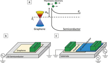
Figure 3a. Equation 2 is derived under the assumption of parabolic energy dispersion for nonrelativistic electrons in a traditional bulk material. For graphene, Equation 2 is no longer valid, and the linear energy dispersion needs to be taken into account. By considering a linear energy dispersion
 ${E_\parallel } = \hbar {v_{\rm{F}}}{k_\parallel }$
, where
 $\hbar$
is the reduced Planck’s constant,
 ${k_\parallel }$
is the in-plane electron wave vector, and
 ${v_{\rm{F}}} = {10^6}$
m/s is the Fermi velocity, in calculating the electron supply function, the RD Law is revised as (termed Dirac-like RD equation):
Reference Liang and Ang31
 $${J_{{\rm{Dirac}}}} = {{ek_{\rm{B}}^3} \over {{{\rm{\pi }}^2}{\hbar ^3}v_{\rm{F}}^2}}{T^3}{e^{ - {{{{\rm{\Phi }}_{\rm{B}}}} \over {{k_{\rm{B}}}T}}}}.$$
(a) Band diagram of graphene/semiconductor Schottky contact (E c and E f denote the semiconductor conduction band edge energy and Fermi level, respectively). The conduction band and valence bands of graphene are denoted by red and blue cones, respectively. (b) Graphene/3D semiconductor Schottky contact. (c) Graphene/2D semiconductor Schottky contact. Note: ΦB, Schottky barrier; V bias, bias voltage; V G, back-gate voltage.

This equation is applicable to both zero-bandgap Dirac dispersion such as in graphene, and finite-bandgap Dirac dispersion such as in MoS2. It is clear that the electron effective mass in the RD Law has been replaced by the Fermi velocity of graphene, circumventing the problematic zero-mass issue – due to the massless nature of graphene’s quasiparticles, Equation 2 would paradoxically dictate the electrical current to be vanishingly small for graphene. Using this equation, better agreement was obtained in a recent experiment Reference Zhu, Lin and Fan54 using a suspended graphene sample. The extracted work function of 4.514 eV is in excellent agreement with experimental measurements Reference Xu, Zeng, Zhang, Ru, Ye, Wang, Seabaugh, Xing, Suehle, Richter, Gundlach and Ngen59 and first-principles calculations. Reference Christodoulou, Giannakopoulos, Nardi, Ligorio, Oehzelt, Chen, Pasquali, Timpel, Giglia, Nannarone, Norman, Linares, Parvez, Mullen, Beljonne and Koch60
Recent experiments have pointed out that the measured Richardson constant is A = 0.02 and 0.024 A/cm2/K2, respectively, for the graphene/Si contact Reference Sinha and Lee57 and the graphene/MoSe2 Reference Sata, Moriya, Morikawa, Yabuk, Masubuchi and Machida61 contact, which are significantly smaller than the theoretical value of 120 A/cm2/K2. Recent experimental studies have also observed spatially inhomogeneous SBH, qualitatively explained by interfacial defects Reference Tomer, Rajput, Hudy, Li and Li62,Reference Tomer, Rajput, Hudy, Li and Li63 and electron–hole puddles—small regions of excess electrons and holes on the graphene plane induced by randomly distributed charge impurities. Reference Martin, Akerman, Ulbricht, Lohmann, Smet, von Klitzing and Yacoby64–Reference Tan, Zhang, Bolotin, Zhao, Adam, Hwang, Das Sarma, Stormer and Kim66 These observations can be explained by a revised Dirac–Schottky diode equation (DSDE): Reference Liang, Hu, Di Bartolomeo, Adam and Ang33
 $${J_{{\rm{DSDE}}}} = {{ek_{\rm{B}}^3} \over {{{\rm{\pi }}^2}{\hbar ^3}v_{\rm{F}}^2}}{T^3}{e^{ - {{{{\rm{\Phi }}_{\rm{B}}} - {{{\rm{\delta }}_{\rm{p}}^2} \over {2{k_{\rm{B}}}T}}} \over {{k_{\rm{B}}}T}}}}\left( {{e^{{{eV} \over {{k_{\rm{B}}}T}}}} - 1} \right)$$
,
where δp estimates the spreading of the Fermi level.
Finally, we briefly discuss Schottky barrier formation mechanism in graphene-based Schottky contacts with either three-dimensional (3D) or 2D semiconductors (Figure 3b–c), because it remains unsolved. By comparing SBH measurements from multiple experiments, Reference Tongay, Lemaitre, Miao, Gila, Appleton and Hebard55,Reference Tomer, Rajput, Hudy, Li and Li63,Reference Kim, Seo, Kim, Song, Suh and Kim67–Reference Rajput, Chen, Liu, Li, Weinert and Li70 the SBH is found to be only weakly correlated to the work function of a 3D semiconductor, but exhibits a much stronger correlation for a 2D semiconductor, Reference Liang, Hu, Di Bartolomeo, Adam and Ang33 which suggests that the effect of Fermi-level pinning is likely to be suppressed in the graphene-2D semiconductor contact. This is in agreement with first-principles calculations Reference Liu, Stadins and Wei71 and offers greater flexibility in engineering the SBH.
Generalized vertical electron emission model for graphene
Not only does the energy dispersion of few-layer graphene (FLG) deviate strongly from its single-layer form, it also depends on the stacking configuration used,
Reference Mak, Shan and Heinz72
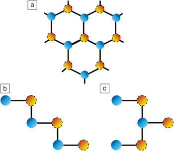
such as ABC or ABA stacking (
Figure 4
). In general, the energy dispersion of ABC-stacked N-layer graphene follows a simple scaling of
 ${E_\parallel } \propto k_\parallel ^N,$
while that of ABA-stacked N-layer graphene is composed of multiple zero-bandgap and finite-bandgap Dirac subbands. By using this relationship, various thermionic emission formulas for FLG with different stacking configurations were obtained (Table I in Reference Reference Ang and Ang32). By using Kane’s nonparabolic energy dispersion, which is widely used to describe the electrons in a narrow bandgap semiconductor,
Reference Kane73
a new Kane–Schottky diode equation
Reference Ang and Ang32
(KSDE) exhibiting a mixture of T
Reference Dushman2
and T
Reference Fowler and Nordheim3
characteristics, is derived as:
 $${J_{{\rm{KSDE}}}} = {{{m^*}ek_{\rm{B}}^2} \over {{{\rm{\pi }}^2}{\hbar ^3}v_{\rm{F}}^2}}\left( {{T^2} + 2{\rm{\gamma }}{k_{\rm{B}}}{T^3}} \right){e^{ - {{{{\rm{\Phi }}_{\rm{B}}}} \over {{k_{\rm{B}}}T}}}}\left( {{e^{ - {{eV} \over {{k_{\rm{B}}}T}}}} - 1} \right)$$
,
which allows the transition between the ultrarelativistic to nonrelativistic limits through a parameter γ. This parameter describes how strongly the energy dispersion deviates from a perfectly parabolic band and is directly related to the bandgap—the strong coupling between conduction and valence bands results in large γ for a very narrow bandgap, whereas γ becomes small for a wide-bandgap semiconductor. For strong nonparabolicity (γ >> 1), T 3-scaling dominates, similar to Equation 3. For perfect parabolicity (γ << 1), the conventional T 2-scaling is recovered.
(a) Crystal structure of graphene. Blue and orange spheres denote the A-sublattice and B-sublattice, respectively. Few-layer graphene (FLG) can be formed by stacking multiple graphene layers. (b–c) Cross-sectional view of a trilayer graphene in ABC and ABA stacking configurations, respectively, which are two of the most thermodynamically stable FLG structures. (b) In the ABC stacking configuration, each graphene layer is shifted by one sublattice in the same direction. (c) In the ABA stacking configuration, the graphene layer is shifted alternately backward and forward by one sublattice.

Finally, based on the same approach, a generalized FN Law for vertical field emission from the graphene plane has been formulated as:
 $${J_{{\rm{Kane}}}} = a\left( {{{{F^2}} \over {\rm{\Phi }}} + {{2{\rm{\gamma }}} \over {{g_{\rm{e}}}}}{{{F^3}} \over {{{\rm{\Phi }}^{3/2}}}}} \right){e^{ - {b \over F}}}$$
,
where
 ${g_{\rm{e}}}$
is a material-dependent parameter. For γ << 1, it reverts to the traditional FN Law. For a nonzero γ, it follows an unconventional form with a F
3 prefactor, which prevents the use of the traditional FN plotting to estimate β.
Conclusion
In summary, we have highlighted some recent developments in thermionic and field emission of electron emission from graphene Reference Liang and Ang31–Reference Liang, Hu, Di Bartolomeo, Adam and Ang33 to show a smooth transition between the nonrelativistic and the relativistic regimes, which will be useful for the development of graphene-based cathodes and engineering of graphene-semiconductor contacts. Many related issues remain unanswered. Why is the field enhancement factor unusually high in graphene (at the edge)? What are the photoemission characteristics of Dirac quasiparticles? For other exotic materials beyond graphene, such as topological insulators in which Dirac electrons and parabolic electrons coexist, Rashba electron gases that have been studied in traditional semiconductor heterostructures and more recently in hybrid organic–inorganic perovskites, the newly discovered Weyl and Dirac semimetals, and few-layer black phosphorus—another emerging class of 2D materials, are the traditional emission models still valid? A recent experiment on photoemission from 3D topological insulators reveals that the long-held belief of spin conservation in photoemission process is no longer valid. This hints that much new physics in this realm remains to be discovered. Reference Jozwiak, Park, Gotlieb, Hwang, Lee, Louie, Denlinger, Rotund, Brgenea, Hssan and Lanzara74
Acknowledgments
This work is supported by the Singapore Ministry of Education T2 Grant (T2MOE1401). L.K.A. acknowledges support from the USA AFOSR AOARD Grant (FA2386–14–1-4020).

Yee Sin Ang is a postdoctoral research fellow at the Singapore University of Technology and Design. He received his bachelor’s degree in medical and radiation physics in 2010, and his PhD degree in theoretical condensed-matter physics in 2014 from the University of Wollongong (UOW), Australia. He received a UOW-EIS Faculty Best Postgraduate Thesis Award and the IPS Meeting Outstanding Poster Award. His research interests include electron emissions from Dirac and spintronic materials, quantum transport in cross-dimensional hybrid interfaces, 2D material valleytronics, and nanoelectronics. Ang can be reached by phone at +65 8715-8088 or by email at yeesin_ang@sutd.edu.sg.

Shi-Jun Liang is a doctoral candidate at the Singapore University of Technology and Design (SUTD). He received his MSc degree in theoretical physics in 2012 from Guangzhou University, China. He is the recipient of the International Vacuum Nanoelectronics Shoulders-Gray-Spindt Award, the IEEE NPSS Graduate Scholarship, and the SUTD FIRST Industry Workshop: Outstanding Graduate Research Award and SUTD President’s Graduate Fellowship Award. His research interests include electron emission from Dirac-type materials, interface issues between different dimensionality materials, plasmonics based on nanostructures, and energy conversion. Liang can be reached by phone at +65 8622-1838 or by email at shijun_liang@mymail.sutd.edu.sg.

Lay Kee (Ricky) Ang has been with the Singapore University of Technology and Design (SUTD) since November 2011, where he is the Ng Teng Fong Professor for the SUTD–Zhejiang University Innovation, Design and Entrepreneurship Alliance; a professor under the Engineering Product Development; and SUTD’s Director of Graduate Studies. He received his BS degree from National Tsing Hua University, Taiwan, in 1994, and his MS and PhD degrees from the University of Michigan in 1996 and 1999, respectively. He has received numerous awards, including the USA ONR Global Visiting Scientist Award and the USA AFOSR AOARD Window of Science Award. His research interests include the quantum model of electron emission, electrical contact, charge transport at interface, novel Dirac material-based devices, and computational methods using fractional models. Ang can be reached by phone at +65 6499-4558 or by email at ricky_ang@sutd.edu.sg.