

1. Introduction
The palaeolatitudinal distribution of climate-sensitive lithologic deposits is important for understanding past climates (Gordon, Reference Gordon1975; Evans, Reference Evans2006; Boucot, Chen & Scotese, Reference Boucot, Chen and Scotese2013), reconstructing palaeogeographies (Ronov, Khain & Seslavinsky, Reference Ronov, Khain and Seslavinsky1984; Ronov, Khain & Balukhovsky, Reference Ronov, Khain and Balukhovsky1989; Scotese Reference Scotese2001, Reference Scotese2004; Golonka et al. Reference Golonka, Krobicki, Pajak, Giang and Zuchiewicz2006; Blakey, Reference Blakey, Fielding, Frank and Isbell2008) and providing constraints for climate modelling (Boucot & Gray, Reference Boucot and Gray2001; Craggs, Valdes & Widdowson, Reference Craggs, Valdes and Widdowson2011) and plate motion histories (Scotese & Barrett, Reference Scotese, Barrett, McKerrow and Scotese1990; Witzke, Reference Witzke, McKerrow and Scotese1990). However, the past distribution of climate-sensitive lithologies remains poorly understood, especially in deep geological times. Latitudinal distribution patterns of palaeoclimate indicators have been considered broadly stable since the Permian, leading to an interpretation that atmospheric and oceanic circulation control their distribution rather than equator-to-pole temperature gradients (Ziegler et al. Reference Ziegler, Eshel, McAllister Rees, Rothfus, Rowley and Sunderlin2003). A global palaeomagnetic compilation of Earth's basin-scale evaporite records suggests that evaporite palaeolatitudes have varied to some degree over the past 2 billion years, with a relatively large difference between Cenozoic–Mesozoic times (a mean palaeolatitude of 23±4°) and Devonian–Ediacaran times (a mean palaeolatitude of 14±2°) (Evans, Reference Evans2006). In addition, previous studies have rarely considered the effect of the uneven distribution of continental areas through time (Vilhena & Smith, Reference Vilhena and Smith2013) and the implications of applying different global tectonic reconstruction models (Scotese & Barrett, Reference Scotese, Barrett, McKerrow and Scotese1990; Ziegler et al. Reference Ziegler, Eshel, McAllister Rees, Rothfus, Rowley and Sunderlin2003) on latitudinal distribution of climate indicators.
In order to better understand the latitudinal distribution patterns of climate-sensitive lithologies and the associated climate change, we revisit a global-scale lithologic compilation of coals, evaporites and glacial deposits, with our analysis extending back to the Devonian period (~400 Ma ago). We test the sensitivity of their latitudinal distribution to uneven distribution of continental areas through time and to reconstruction models, and then quantify their distribution patterns with corrections of sampling- and continental area-bias, using Significant Zero crossings of the derivative (SiZer) of Chaudhuri & Marron (Reference Chaudhuri and Marron1999) to obtain the best-fitting probability density functions and Highest Density Regions (HDR) of Hyndman (Reference Hyndman1996) to compute 50% and 95% confidence intervals. The shifting latitudinal distribution patterns reflect climate change associated with humid/arid, precipitation/evaporation or cold/warm climatic conditions. To understand the mechanism, we compare the trends of latitudinal distribution patterns of these palaeoclimate deposits with the atmospheric CO2 evolution (Foster, Royer & Lunt, Reference Foster, Royer and Lunt2017) and tropic mountain range areas derived from the palaeogeographic maps (Golonka et al. Reference Golonka, Krobicki, Pajak, Giang and Zuchiewicz2006; Cao et al. Reference Cao, Zahirovic, Flament, Williams, Golonka and Müller2017) over time, as increased silicate weathering rates associated with tropical mountain uplift lead to a decrease in atmospheric CO2 concentration and this may initiate glaciation (Tabor & Poulsen, Reference Tabor and Poulsen2008; Montañez & Poulsen, Reference Montañez and Poulsen2013; Goddeŕis et al. Reference Godderis, Donnadieu, Carretier, Aretz, Dera, Macouin and Regard2017; Swanson-Hysell & Macdonald, Reference Swanson-Hysell and Mac Donald2017).
2. Data and global plate tectonic models
We use a dataset of climate-sensitive lithologies, including coals, evaporites and glacial deposits (tillites, dropstones and glendonites), based on a comprehensive global-scale compilation (Boucot, Chen & Scotese, Reference Boucot, Chen and Scotese2013). This compilation records and evaluates various types of climatically sensitive lithologic deposits, including coal, cyclothems, laterite, bauxite, lateritic manganese, oolitic ironstone, kaolinite, glendonite, tillites, dropstones, calcretes, evaporites, clay minerals, palms, mangroves and crocodilians, based on a comprehensive literature review. It covers geological times from the Cambrian period to the Miocene epoch. Each data point includes a reference source and geographic location. In order to analyse the effect of global climate change on the latitudinal distribution patterns of climate-sensitive lithologies, we use recorded occurrences of coals, (mostly marine) evaporites, and glacial deposits (a combination of tillites, dropstones and glendonites) in this study, as distributions of other lithologies included in the database are less reliable latitude indicators. For instance, the record of palms, mangroves and crocodilians suffers from sampling bias as they are mostly collected from middle–high latitudes, while sample sizes are small for laterites and oolitic ironstones.
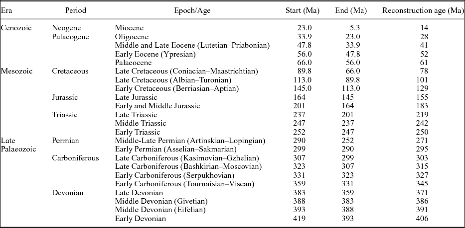
The dataset used in this study covers Devonian to Miocene times and is divided into 23 time intervals at the scale of geological stages (Table 1). The time range that we assign to each data point is entirely derived from the time ranges that Boucot, Chen & Scotese (Reference Boucot, Chen and Scotese2013) used to draw the maps, and we use the middle ages of these time intervals to determine the reconstruction times (Table 1). We use modern peats (as they may eventually become coals), evaporites and glacial sediments (tillites and ‘glacio-marine’ beds) from Ziegler et al. (Reference Ziegler, Eshel, McAllister Rees, Rothfus, Rowley and Sunderlin2003) for reference. Coals and peats are generally considered as indicators of terrestrial humidity, reflecting climatic regimes in which precipitation exceeds or is equal to evaporation (Parrish, Ziegler & Scotese, Reference Parrish, Ziegler and Scotese1982; Hallam, Reference Hallam1985; McCabe & Parrish, Reference McCabe, Parrish, McCabe and Parrish1992; Price, Sellwood & Valdes, Reference Price, Sellwood and Valdes1995). Evaporites are formed in climatic conditions where evaporation exceeds the combined effects of precipitation, marine or river influx, and runoff (Craggs, Valdes & Widdowson, Reference Craggs, Valdes and Widdowson2011), yet, they may occur in temperate regions (Boucot, Chen & Scotese, Reference Boucot, Chen and Scotese2013). Tillites, dropstones and glendonites in the dataset are glacial or glacial-origin deposits indicating cold climate, generally due to high latitudes, but some could be related to high elevations (Boucot, Chen & Scotese, Reference Boucot, Chen and Scotese2013).
Time division of the climate-sensitive lithologic indicators of Boucot, Chen & Scotese (Reference Boucot, Chen and Scotese2013) using the 2016 timescale of the International Commission on Stratigraphy (ICS2016). The reconstruction age is the rounded-off middle age of each time interval.

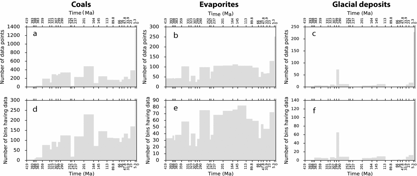
The climatically sensitive lithologic deposits are distributed unevenly over different time intervals (Figs 1, 2). There are very few records of coals in the Devonian period (Figs 1, 2), with coals largely occurring in the Late Devonian stratigraphies (Boucot, Chen & Scotese, Reference Boucot, Chen and Scotese2013). Yet a large number of coal records appear in Carboniferous, Permian, Late Triassic, Early Jurassic and Neogene times (Figs 1, 2a). Evaporites have relatively uniform richness over most of the time intervals, except in Devonian, Late Carboniferous, Early Permian and Palaeogene times (Figs 1, 2b), whereas, glacial deposit records are relatively rare and sparse over time (Figs 1, 2c) due to the dominance of greenhouse conditions in the Phanerozoic (Hay, Reference Hay2016).
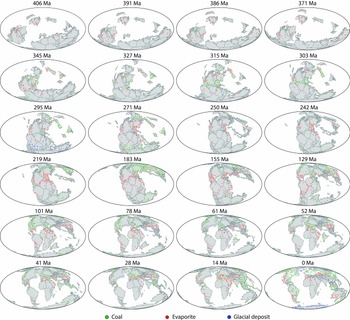
Locations of climate-sensitive lithologic data reconstructed using the plate motion model of Matthews et al. (Reference Matthews, Maloney, Zahirovic, Williams, Seton and Müller2016): coals (green), evaporites (red) and glacial deposits (blue) since the Early Devonian (Ziegler et al. Reference Ziegler, Eshel, McAllister Rees, Rothfus, Rowley and Sunderlin2003; Boucot, Chen & Scotese, Reference Boucot, Chen and Scotese2013). Ages at the top of each panel are reconstruction ages according to the timescale described in Table 1.

(a, b, c) Sum of data points of coals, evaporites and glacial deposits at each time interval since the Devonian period. (d, e, f) Sum of resampled data points for coals, evaporites and glacial deposits at each time interval since the Devonian period.

In this study, we primarily use the global plate tectonic model of Matthews et al. (Reference Matthews, Maloney, Zahirovic, Williams, Seton and Müller2016) to reconstruct the lithologic data points back in time from present-day geographic locations. This tectonic model represents a combination of a tectonic model for Mesozoic and Cenozoic times (230–0 Ma) (Müller et al. Reference Müller, Seton, Zahirovic, Williams, Matthews, Wright, Shephard, Maloney, Barnett-moore, Bower and Cannon2016) and a tectonic model for Palaeozoic times (410–250 Ma) (Domeier & Torsvik, Reference Domeier and Torsvik2014), with a number of changes required to enable a smooth merging of the models as described by Matthews et al. (Reference Matthews, Maloney, Zahirovic, Williams, Seton and Müller2016). It is a relative plate motion model that is ultimately tied to Earth's spin axis through an absolute reference frame (Matthews et al. Reference Matthews, Maloney, Zahirovic, Williams, Seton and Müller2016). We removed the true polar wander correction from the original absolute plate motion model (Domeier & Torsvik, Reference Domeier and Torsvik2014) to tie the relative rotations to a palaeomagnetic reference frame. Therefore, the tectonic reconstruction better reflects the true palaeolatitudinal distribution of palaeoclimate indicators (van Hinsbergen et al. Reference van Hinsbergen, de Groot, van Schaik, Spakman, Bijl, Sluijs, Langereis and Brinkhuis2015).
In order to test the sensitivity of the palaeolatitudinal distribution of climate-sensitive deposits to the choice of reconstruction model, except for the plate motion model of Matthews et al. (Reference Matthews, Maloney, Zahirovic, Williams, Seton and Müller2016), we use two alternative reconstruction models of Scotese (Reference Scotese2008) and Golonka (Reference Golonka2007) which are both based on the reconstruction of Scotese (Reference Scotese2004). The reconstruction model of Golonka (Reference Golonka2007) uses palaeomagnetic data to constrain the palaeolatitudinal positions of continents and rotation of plates, and hot spots, where applicable, are used as reference points to calculate palaeolongitudes. A version of this model that includes an updated absolute reference frame is described in Wright et al. (Reference Wright, Zahirovic, Müller and Seton2013), and the model is available in the supplementary materials of Wright et al. (Reference Wright, Zahirovic, Müller and Seton2013). The reconstruction model of Scotese (Reference Scotese2008) uses palaeomagnetic reference frames for 410–250 Ma (Ziegler et al. Reference Ziegler, Scotese, McKerrow, Johnson and Bambach1979) and 250–100 Ma (Ziegler, Scotese & Barrett, Reference Ziegler, Scotese, Barrett, Brosche and Sündermann1983), and a hotspot reference frame for 100–0 Ma (Müller, Royer & Lawver, Reference Müller, Royer and Lawver1993).
3. Methods
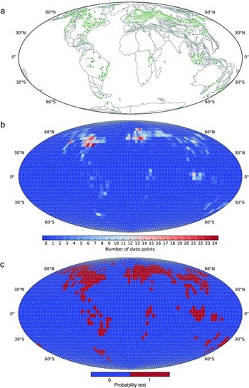
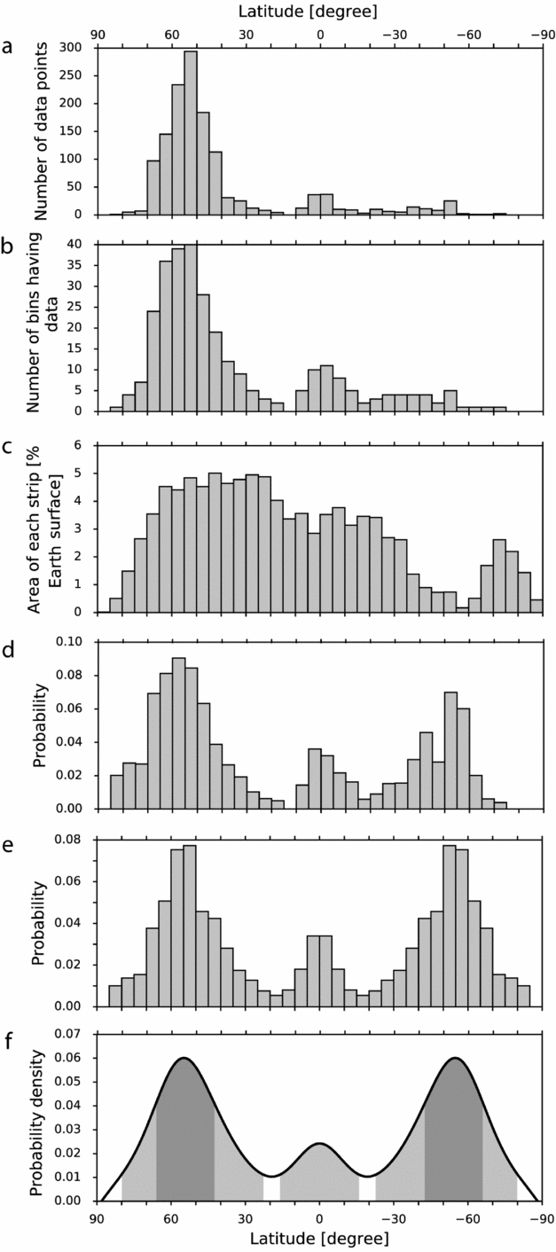
We first reconstructed the lithologic data for coals, evaporites and glacial deposits from their modern locations to ancient locations in geological time (Fig. 1) using the global plate motion model of Matthews et al. (Reference Matthews, Maloney, Zahirovic, Williams, Seton and Müller2016). Due to the inconsistency of age assignments between some lithologic data and “underlying” terrane polygons, leading to unexpected reconstructed locations of these lithologic data, we only considered the data points whose time ranges of existence were within the time span and present-day spatial extent of the underlying terrane. We next binned the data points using a 5° × 5° mesh of the global surface, following Ziegler et al. (Reference Ziegler, Eshel, McAllister Rees, Rothfus, Rowley and Sunderlin2003) (Fig. 3b). Each bin contained a variable number of data points or none; for example, a bin could contain 0–24 data point(s) for modern peats at present-day coordinates (Fig. 3b). The recorded data points were unevenly distributed spatially (Fig. 3a, b), largely due to sampling bias. To remove the bias, we resampled the data by collapsing all the samples into a single value for each bin: 1 where data existed (Fig. 3c, red bins), and 0 where there were no data points (Fig. 3c, blue bins). We subsequently summed up the numbers of resampled data in each 5° latitudinal strip (Fig. 4b). These steps significantly reduced the numbers of data points considered per latitudinal strip (compare the y-axis of Fig. 4a, b).
(a) Present-day locations of modern global peats (green points) from Ziegler et al. (Reference Ziegler, Eshel, McAllister Rees, Rothfus, Rowley and Sunderlin2003). Grey polygons are modern terrane geometries. (b) Distribution of modern peat points binned using a 5°×5° mesh of the global surface. (c) Distribution of resampled modern peat points (red: bins containing at least one data point; blue: bins containing no data points).

(a) Number of original modern peat points from Ziegler et al. (Reference Ziegler, Eshel, McAllister Rees, Rothfus, Rowley and Sunderlin2003) in each 5° latitudinal strip. (b) Number of resampled modern peat points in each 5° latitudinal strip. (c) Modern continental area in each 5° latitudinal strip as a percentage of total modern continental area. (d) Distribution of resampled modern peat points with continental area bias corrected. (e) Distribution of modern peat points with sampling- and area-biases corrected. The two hemispheres are combined to form a symmetric distribution pattern (also known as zonal pattern; Scotese & Barrett, Reference Scotese, Barrett, McKerrow and Scotese1990; Ziegler et al. Reference Ziegler, Eshel, McAllister Rees, Rothfus, Rowley and Sunderlin2003). (f) Fitted probability density function (black line) using the method of SiZer from Chaudhuri & Marron (Reference Chaudhuri and Marron1999). High-density latitude ranges at confidence intervals of 50% (grey area) and 95% (light grey area) using the HDR method of Hyndman (Reference Hyndman1996).

Plate tectonic motion (Golonka, Reference Golonka2007; Scotese, Reference Scotese2008; Matthews et al. Reference Matthews, Maloney, Zahirovic, Williams, Seton and Müller2016) leads to a biased distribution of lithologic deposits on Earth. Latitude bands containing more continental area are more likely to have more lithologic deposits preserved. In an attempt to remove this bias, we first calculated the continental area covered by each 5° latitudinal strip at each time interval since the Devonian period (Fig. 4c), using the HEALPix pixelization method that results in equal sampling of data on a sphere (Goŕski et al. 2005) and therefore equal sampling of surface areas. We next corrected the number of resampled lithologic data in a 5° latitudinal strip using the continental area in the same strip to remove the bias due to the uneven distribution of continental areas through time. Subsequently, the results were scaled to represent probabilities of data appearing in a 5° latitudinal strip (Fig. 4d). In order to investigate the palaeolatitudinal zonal patterns of these climate indicators, we combined the data corrected for continental area bias from both hemispheres to form symmetric and composite zonal patterns, and normalized the results in a strip into probabilities with respect to the sum of all the values in the same strip (Fig. 4e). The symmetric zonal patterns erased the differences between the two hemispheres and can be used to indicate the influence of climate change on the distribution of climate-sensitive lithologic deposits (Scotese & Barrett, Reference Scotese, Barrett, McKerrow and Scotese1990; Ziegler et al. Reference Ziegler, Eshel, McAllister Rees, Rothfus, Rowley and Sunderlin2003).
We used SiZer (SIgnificant ZERo crossing of the derivatives; by Chaudhuri & Marron, Reference Chaudhuri and Marron1999), a data analysis method to identify significant peaks from kernel density estimation to obtain probability density functions of zonal patterns (Fig. 4f, black lines). Instead of trying to find the one bandwidth that provides the closest match to the unknown true density, SiZer looks at the whole range of bandwidths. Peaks and troughs are identified by finding the regions of significant gradient (zero crossings of the derivative; Chaudhuri & Marron, Reference Chaudhuri and Marron1999). In order to identify high-density intervals of distribution of these palaeoclimate indicators, we used the HDR method of Hyndman (Reference Hyndman1996) to compute the high-density latitude ranges with 50% (Fig. 4f, grey area) and 95% (Fig. 4f, light grey area) confidence intervals. HDR is a statistical method for calculating confidence intervals when the sampling distribution has multiple peaks. For discrete-valued distribution, HDR simply consists of those elements of the sample space with highest probability (Hyndman, Reference Hyndman1996).
4. Results
4.a. Palaeolatitudinal distribution of coals, evaporites and glacial deposits
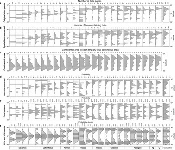
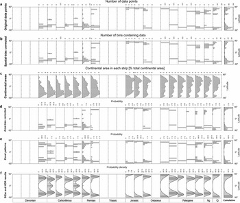
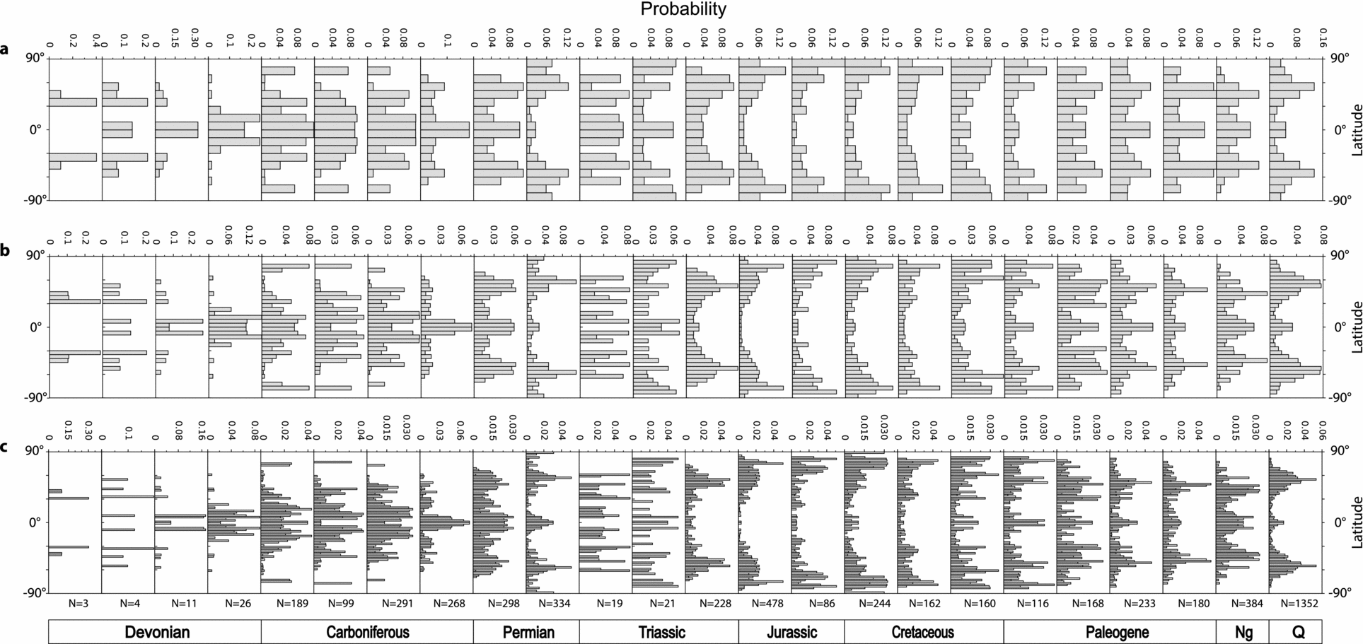
We counted the original data points for coals (Fig. 5a), evaporites (Fig. 6a) and glacial deposits (Fig. 7a) reconstructed using the plate tectonic model of Matthews et al. (Reference Matthews, Maloney, Zahirovic, Williams, Seton and Müller2016) in each 5° latitudinal strip at each time interval since the Devonian period. Coals are distributed in a wide latitude range from the equator to the poles (Fig. 5a), while evaporites are concentrated between 60°N and 60°S (Fig. 6a). Glacial deposits generally occur in middle–high latitudes except for a record of glendonites appearing near the equator in the Early Carboniferous (Tournaisian–Visean) from an outer shelf environment with near-0°C seawater (Brandley & Krause, Reference Brandley and Krause1993a, Reference Brandley and Krauseb, Reference Brandley, Krause, Embry, Beauchamp and Glass1994), a record of tillites in the Late Carboniferous (Kasimovian–Gzhelian) and a record of tillites in the Early Permian, both from a high-elevation periglacial environment (Becq-Giraudon, Montenat & Van den Driessche, Reference Becq-Giraudon, Montenat and Van Den Driessche1996) (Fig. 7a). Therefore, these three records (highlighted with question marks in Fig 7) may not be reliable enough to indicate cold climate relevant to latitudinal change.
(a) Numbers of original coal points of Boucot, Chen & Scotese (Reference Boucot, Chen and Scotese2013) and Ziegler et al. (Reference Ziegler, Eshel, McAllister Rees, Rothfus, Rowley and Sunderlin2003) reconstructed using the tectonic model of Matthews et al. (Reference Matthews, Maloney, Zahirovic, Williams, Seton and Müller2016) in each 5° latitudinal strip for each time interval since the Devonian period. (b) Number of resampled coal points in each 5° latitudinal strip for each time interval. (c) Continental area in each 5° latitudinal strip as a percentage of Earth's surface for each time interval. (d) Distribution of coals with continental area corrected in each 5° latitudinal strip for each time interval. (e) Symmetric zonal pattern of coals with sampling- and continental area-biases removed. (f) Probability density function of symmetric zonal pattern of coals for each time interval. The cumulative results for all times are presented on the rightmost side with bold borders.

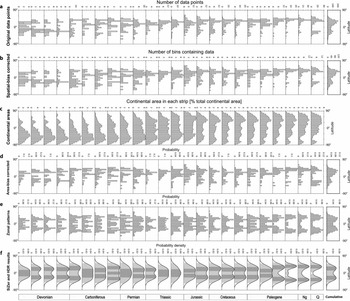
(a) Number of original evaporate points of Boucot, Chen & Scotese (Reference Boucot, Chen and Scotese2013) and Ziegler et al. (Reference Ziegler, Eshel, McAllister Rees, Rothfus, Rowley and Sunderlin2003), reconstructed using the tectonic model of Matthews et al. (Reference Matthews, Maloney, Zahirovic, Williams, Seton and Müller2016), in each 5° latitudinal strip for each time interval since the Devonian period. (b) Number of resampled evaporate points in each 5° latitudinal strip for each time interval. (c) Continental area in each 5° latitudinal strip as a percentage of total continental area for each time interval. (d) Distribution of evaporites with continental area corrected in each 5° latitudinal strip for each time interval. (e) Zonal pattern of evaporites with sampling- and continental area-biases corrected. (f) Probability density function of zonal pattern of evaporites for each time interval. The cumulative results for all times are presented on the rightmost side with bold borders.

(a) Numbers of original glacial deposit points of Boucot, Chen & Scotese (Reference Boucot, Chen and Scotese2013) and Ziegler et al. (Reference Ziegler, Eshel, McAllister Rees, Rothfus, Rowley and Sunderlin2003) reconstructed using the tectonic model of Matthews et al. (Reference Matthews, Maloney, Zahirovic, Williams, Seton and Müller2016) in each 5° latitudinal strip for each time interval since the Devonian period. (b) Number of resampled glacial deposit points in each 5° latitudinal strip for each time interval. (c) Continental area in each 5° latitudinal strip as a percentage of total continental area for each time interval. (d) Distribution of glacial deposit with continental area corrected in each 5° latitudinal strip for each time interval. (e) Zonal pattern of glacial deposit with sampling- and continental area-biases corrected. (f) Probability density function of zonal pattern of glacial deposits for each time interval. The troughs with a question mark indicate records unlikely to represent latitudinal changes in climate. The cumulative results for all times are presented on the far right with bold borders.

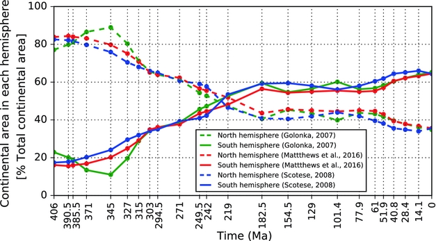
Generally, more data points of coals (Fig. 5a), evaporites (Fig. 6a) and glacial deposits (Fig. 7a) are sampled from the northern than the southern hemisphere since Pangaea break-up in the Early Jurassic (Ronov, Khain & Seslavinsky, Reference Ronov, Khain and Seslavinsky1984; Ronov, Khain & Balukhovsky, Reference Ronov, Khain and Balukhovsky1989; Scotese, Reference Scotese2001, Reference Scotese2004; Golonka et al. Reference Golonka, Krobicki, Pajak, Giang and Zuchiewicz2006; Blakey, Reference Blakey, Fielding, Frank and Isbell2008). During Early Devonian – Late Triassic time, the numbers of data points of these lithologies in the southern hemisphere exceed those in the northern hemisphere in general, with glacial deposits only occurring in the southern hemisphere in Early Devonian and Carboniferous times (Fig. 7a). This mainly reflects the fact that plate tectonic motions modify the continental configuration through time, which has led to more continental areas in the northern hemisphere since the Early Jurassic (Figs 5c, 8). Continental areas in the northern hemisphere have consistently increased since the Devonian period, while the areas in the southern hemisphere have decreased accordingly (Figs 5c, 8).
Continental area in the northern and southern hemispheres respectively as a percentage of total continental area at each time interval since the Devonian period.

After removing the sampling- (Figs 5b, 6b, 7b) and continental area-biases (Figs 5d, 6d, 7d) over the data in each 5° strip at each time interval, the differences among strips at a time interval are evened out to some degree (for example, compare the y-axis of Fig. 5a, b, d). The zonal patterns for coals (Fig. 5e), evaporites (Fig. 6e) and glacial deposits (Fig. 7e) vary considerably over time.
We compute the high-density latitudinal ranges with 50% and 95% confidence intervals for coals (Fig. 5f), evaporites (Fig. 6f) and glacial deposits (Fig. 7f), respectively, at each time interval. Considering the extent of these 95% confidence ranges, coals are relatively widely distributed on Earth's surface over the time period of interest, extending from the equator to the poles for many time periods (Fig. 5f, light grey area). Evaporites (95% confidence) are generally concentrated within low–middle latitudes (0–60°) in two hemispheres, with a mean palaeolatitude of 26±3° in each hemisphere since the Devonian (Fig. 6f, light grey area). This result is consistent with the mean palaeolatitudes of 23±4° during Cenozoic–Mesozoic time and 21±4° during Permian–Carboniferous time (both with 95% confidence), recalculated from palaeolatitudes of a global compilation of large evaporite basins extending back through Proterozoic time (Evans, Reference Evans2006). Glacial deposits (95% confidence) occur in Late Devonian, Carboniferous, Permian, Jurassic, Early Cretaceous and Late Palaeogene–modern times (Fig. 7f, light grey area). This is generally consistent with three main Phanerozoic ice ages during Carboniferous–Permian, Late Jurassic – early Cretaceous and Early Eocene–modern times (Frakes, Francis & Syktus, Reference Frakes, Francis and Syktus1992).
Focusing on 50% confidence intervals, coal latitudinal belts show strong fluctuation over time (Fig. 5f, dark grey area). They move from the middle latitudes towards the equator during the Devonian, but the original coal deposits in the Devonian are too few to provide much climatological insight (Boucot, Chen & Scotese, Reference Boucot, Chen and Scotese2013). During the Carboniferous, they are strictly limited within 0–25°N and S; however, they separate into two latitudinal belts of 0–10° and 40–60° during the earliest Permian (Asselian–Sakmarian) (Fig. 5f). Subsequently, they undergo a poleward shift until reaching higher latitudes (60–90°) during the Late Jurassic, with a sharp equatorward movement in the Early Triassic and a rapid poleward shift in the Middle Triassic but these may be not reliable as they are based on very few data points (Figs 1, 2a). Starting from the Early Cretaceous, the distributions of coals contract towards the equator until the Miocene when there are two latitudinal belts at ~30–50° and ~0–15° on two hemispheres, with a rapid shift towards the equator during the Early Eocene. Modern peats are mainly distributed within ~40–65° latitudes. Overall, the latitudinal belts determined for coals from probability density curves with 50% confidence generally occur at low latitudes during Palaeozoic time, middle latitudes during Permian, Triassic and Cenozoic times, and high latitudes during Jurassic and Cretaceous times.
Evaporite latitudinal belts with 50% confidence (Fig. 6f, grey area) mostly occur at low latitudes (~0–30°N and S). They move poleward from the Early Devonian until the Early Carboniferous and then towards the equator until the Late Triassic. Starting from the Middle Triassic, they start to shift poleward until modern times at a mean latitude of ~35°N and S, with a short and rapid poleward movement during the early Eocene (Lutetian).
The trends in how the highest-density latitudes of glacial deposits with 50% confidence (Fig. 7f, grey area) shift northwards or southwards are similar to coals, but at higher latitude. They generally concentrate within middle–high latitudes through time (Fig. 7, grey area). They occur at ~50–70°N and S latitudes during the Late Devonian and then move equatorward to middle latitudes (~40–60°) during most of the Carboniferous, with a rapid poleward movement in the Late Mississippian. The Late Pennsylvanian – Early Permian transition is marked by a rapid shift of glacial deposits towards high latitudes. They remain at high latitudes during Jurassic and Cretaceous times, and then move to middle–high latitudes (~50–75°) during Palaeogene and Miocene times. Modern glacial deposits mainly lie near the poles.
4.b. Sensitivity tests
4.b.1. Assumption of climate symmetry (zonal patterns)
In order to test the assumption that past climates were zonal and hemispherically symmetric, we investigated the latitudinal distributions of lithologies for each hemisphere independently through time, and estimated their high-density latitudinal belts using the same statistical methods (Supplementary Figs S1 and S2, available at https://doi.org/10.1017/S0016756818000110). At the first order, more lithologic data are distributed on the northern hemisphere over the timeframe, except for late Palaeozoic and Cenozoic times when more glacial deposits formed in the southern hemisphere. The distributions of coals and evaporites in the northern hemisphere (Supplementary Figs S1 and S2, available at https://doi.org/10.1017/S0016756818000110) are similar to the results with data combined over two hemispheres (Fig. 12a, c, further below). This is largely because of the uneven distribution of continental areas through time, leading to a biased distribution of lithologic deposits in the northern hemisphere. Overall, the data distribution warrants combining the two hemispheres in zonal patterns.
4.b.2. Continental area bias
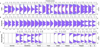
In order to examine sensitivity of the zonal patterns of these lithologic deposits to continental area bias, we compute the zonal patterns for coals (Fig. 9a), evaporites (Fig. 9b) and glacial deposits (Fig. 9c) for each time interval since the Devonian using the plate motion model of Matthews et al. (Reference Matthews, Maloney, Zahirovic, Williams, Seton and Müller2016) with (Fig. 9, blue area) and without (Fig. 9, red) continental area correction, respectively. The distribution patterns of coals using the two approaches are significantly different in Middle Devonian, most of Carboniferous, Early and Middle Triassic, Jurassic, Cretaceous and Early Palaeogene times. During these time periods except the Middle Devonian, the zonal patterns of coals without continental area correction are closer to the equator (Fig. 9, red). This mainly results from the uneven latitudinal distribution of continental areas, with very little to no continental coverage near the poles during these periods (Fig. 5c). Due to relatively small continental coverage near the equator (Fig. 5c), the zonal patterns of coals without area correction are closer to the poles during the Middle Devonian (Fig. 9, red).
Zonal patterns of lithologic deposits of coals (a), evaporites (b) and glacial deposits (c), with continental area bias correction (blue) and without continental area bias correction (red), for each time interval since the Devonian period using the plate motion model of Matthews et al. (Reference Matthews, Maloney, Zahirovic, Williams, Seton and Müller2016). The number of original data points at each time interval is reported at the bottom of each subplot.

The uneven distribution of continental areas through time has relatively less impact on the zonal patterns of evaporites (Fig. 9b) and glacial deposits (Fig. 9c). Evaporite zonal patterns are generally identical over time, except during Late Mississippian, Late Pennsylvanian, the earliest Permian, Middle Triassic and late Cretaceous times (Fig. 9b). Due to different continental coverage at different latitudes (Fig. 5c), the area correction leads to more poleward distributions of evaporites during Late Mississippian, Late Pennsylvanian and earliest Permian times but more equatorward during Middle Triassic and late Cretaceous times. With and without area correction, glacial deposit zonal patterns are mostly identical over time, except for most of Permian, Late Palaeogene and modern times, when the area correction results in more poleward distributions, and for Early and Late Mississippian and Late Pennsylvanian times, with more equatorward distributions (Fig. 9c). Overall, latitudinal distributions of coals show stronger sensitivity to uneven distributions of continents than evaporites and glacial deposits, which could be mainly due to coals having a wider latitudinal distribution than evaporites and glacial deposits over time.
4.b.3. Reconstruction model bias
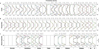
We use alternative reconstruction models of Scotese (Reference Scotese2008) and Golonka (Reference Golonka2007) with modifications as described in Wright et al. (Reference Wright, Zahirovic, Müller and Seton2013), in addition to the model of Matthews et al. (Reference Matthews, Maloney, Zahirovic, Williams, Seton and Müller2016), to analyse the sensitivity of latitudinal distributions of coals, evaporites and glacial deposits to the reconstruction model. We use the same method described in the Methods section to obtain the probability density functions of the latitudinal distributions for these lithologies over time. The results indicate that the three reconstructions result in only second-order differences through time (Fig. 10). Differences in the distributions are most pronounced where reconstructed palaeolatitudes differ for blocks that host a large proportion of data points for a given time interval.
Latitudinal distribution of coals (a), evaporites (b) and glacial deposits (c), for each time interval since the Devonian period, using three reconstruction models (blue: Matthews et al. Reference Matthews, Maloney, Zahirovic, Williams, Seton and Müller2016; red: Scotese, Reference Scotese2008; green: Golonka, Reference Golonka2007). The number of original data points at each time interval is reported at the bottom of each subplot.

The latitudinal distributions of coals reconstructed using the three tectonic models are generally similar over time, except during Early Devonian, Early Carboniferous, the earliest Permian, Middle and Late Palaeogene and Neogene times. In the Early Devonian, the latitudinal distributions of coals using the reconstruction of Golonka (Reference Golonka2007) are more northward than those using the other two reconstructions, largely because North America and Eurasia in the model of Golonka (Reference Golonka2007) are located further northward than in the other two models during this period (see Supplementary Material available at https://doi.org/10.1017/S0016756818000110). The more poleward location of Africa during the Early Carboniferous in the reconstruction of Matthews et al. (Reference Matthews, Maloney, Zahirovic, Williams, Seton and Müller2016) leads to a more poleward distribution of coals. During the earliest Permian, numerous coal deposits occur in North and South China blocks. Their more northward locations in the model of Matthews et al. (Reference Matthews, Maloney, Zahirovic, Williams, Seton and Müller2016), taken from the work of Domeier & Torsvik (Reference Domeier and Torsvik2014), result in more occurrences at middle latitudes (see Supplementary Material available at https://doi.org/10.1017/S0016756818000110). The terranes in the reconstruction of Scotese (Reference Scotese2008) are generally further north relative to the other two models during Middle and Late Palaeogene and Neogene times (see Supplementary Material available at https://doi.org/10.1017/S0016756818000110). This results in more poleward distributions of overall palaeoclimate lithologies (Fig. 10a).
The latitudinal distributions of evaporites among the three reconstructions are very similar since the Devonian (Fig. 10b), except for Early Devonian and Carboniferous times. In the Early Devonian, evaporites are spread further from the equator using the reconstruction of Golonka (Reference Golonka2007) than the other two reconstructions, which is mainly due to more northward locations of North America and Eurasia in the model of Golonka (Reference Golonka2007). More southward locations of numerous plates in the reconstruction of Golonka (Reference Golonka2007) (see Supplementary Material available at https://doi.org/10.1017/S0016756818000110) result in more equatorial distributions of evaporites during the Carboniferous (Fig. 10b).
The latitudinal distributions of glacial deposits are also similar through time among the three considered reconstructions (Fig. 9c), except for the Late Devonian, Early and Middle Mississippian and most of the Permian. During the Late Devonian, more glacial deposits are distributed at high latitudes using the reconstruction of Scotese (Reference Scotese2008), mainly due to the more southerly location of South America in this reconstruction than that in the other two reconstructions (see Supplementary Material available at https://doi.org/10.1017/S0016756818000110). The more equatorial locations of South America and NW Africa in the model of Scotese (Reference Scotese2008) lead to more equatorial distributions of glacial deposits during Early and Middle Mississippian times. During most of the Permian period, Antarctica and Australia are closer to the South Pole in the reconstruction of Golonka (Reference Golonka2007) (see Supplementary Material available at https://doi.org/10.1017/S0016756818000110), resulting in more poleward distribution of glacial deposits (Fig. 10c).
4.b.4. Spatial sampling resolution bias
We compare the use of three different spatial resolutions to bin the original data points to remove the effect of sampling bias on the distribution patterns of these climatically lithologic deposits, using the plate motion model of Matthews et al. (Reference Matthews, Maloney, Zahirovic, Williams, Seton and Müller2016), for each time interval since the Devonian period: 10° (Fig. 11a), 5° (Fig. 11b) and 2° (Fig. 11c). The results indicate that there are too few strips containing data points, especially during the Devonian, to be able to obtain much statistical significance using 10° as the binning size (Fig. 11a). Using 2° as the binning size results in noisier distributions (Fig. 11c) and a more difficult analysis of distribution patterns. A spatial resolution of 5° is a good compromise that captures the data distribution yet results in less noise, and follows previous work that aids comparison with our work (Fig. 11b).
Distribution patterns of coals, reconstructed using the plate motion model of Matthews et al. (Reference Matthews, Maloney, Zahirovic, Williams, Seton and Müller2016), for each time interval since the Devonian period using three different bin sizes (red: 10° (a); blue: 5° (b); green: 2° (c)) to bin data points to in order to remove the sampling bias. The number of original data points at each time interval is reported at the bottom of each subplot.

5. Discussion
5.a. Palaeolatitudinal distribution patterns of lithologic climate indicators over time
We present the high-density latitudinal ranges in one hemisphere, due to the assumed symmetry of two hemispheres, with 50% and 95% confidence intervals for coals (Fig. 12a), evaporites (Fig. 12b) and glacial deposits (Fig. 12c), respectively, at each time interval. We also present the cumulative high-density latitudinal ranges over the entire time period for these lithologies (rightmost panels in Fig. 12a, b, c). Overall, the latitudinal belts determined from probability density curves with 50% confidence for coals have changed since the Devonian. Some previous studies concluded that the palaeolatitudinal distribution of coals has remained broadly similar since the Permian (Ziegler et al. Reference Ziegler, Eshel, McAllister Rees, Rothfus, Rowley and Sunderlin2003), whereas we have shown that results for earlier in the Palaeozoic are significantly different from results from the Permian to present (Fig. 12a, b, c). In addition, the temporal division at the scale of geological periods in previous studies did not attempt to resolve variations over shorter time periods, whereas the dataset used in this study is based on a time division at the scale of geological stages. The temporal resolution based on the scale of geological periods does not allow us to capture variations of latitudinal distribution patterns of climate-sensitive lithologic deposits within geological periods, such as the significant movement towards the equator from probability density curves with 50% confidence for coals between Early Palaeogene and Middle Palaeogene times in Figure 12a.
(a, b, c) High-density latitudinal belts of coals, evaporites and glacial deposits, with 50% (blue area) and 95% (light grey area) confidence intervals for each time interval since the Devonian period. The blue lines are the most significant peaks of latitudinal distribution. The areas with a question mark indicate records of limited use for climate interpretation. Cumulative high-density probabilities are presented on the rightmost side with bold borders. (d) Atmospheric CO2 concentration curve since the Devonian period, derived from Foster, Royer & Lunt (Reference Foster, Royer and Lunt2017). 68% and 95% confidence intervals are shown as dark and light grey bands. The blue line represents a locally weighted scatterplot smoothing (LOESS) fit, a nonparametric regression fit from Cleveland & Devlin (Reference Cleveland and Devlin1988), through the data. Icehouse intervals and greenhouse intervals (Hay, Reference Hay2016) are indicated by a blue band and a white band, respectively, at the top of the panel. (e) Global palaeolatitudinal distribution of mountain ranges since the Devonian period calculated from the set of palaeogeographic maps (Golonka et al. Reference Golonka, Krobicki, Pajak, Giang and Zuchiewicz2006; Cao et al. Reference Cao, Zahirovic, Flament, Williams, Golonka and Müller2017). (f) Global palaeolatitudinal distribution of shallow marine environments (Golonka et al. Reference Golonka, Krobicki, Pajak, Giang and Zuchiewicz2006; Cao et al. Reference Cao, Zahirovic, Flament, Williams, Golonka and Müller2017). (g) Global palaeolatitudinal distribution of ice sheets from the palaeogeographic maps (Golonka et al. Reference Golonka, Krobicki, Pajak, Giang and Zuchiewicz2006; Cao et al. Reference Cao, Zahirovic, Flament, Williams, Golonka and Müller2017). (h) Climate temperature gradients since the Early Devonian derived from Boucot, Chen & Scotese (Reference Boucot, Chen and Scotese2013).

Highest-density latitudinal belts of evaporites with 50% confidence exhibit relatively subtle shifts within a narrow range of latitudes over time (Fig. 12b), although they are very similar to the cumulative result covering the entire temporal range (right panel in Fig. 12b). Evans (Reference Evans2006) suggested that evaporite palaeolatitudes remain stable during Cenozoic–Mesozoic times (a mean palaeolatitude of 23±4°) and during Devonian–Ediacaran times (a mean palaeolatitude of 14±2°). This might be because the time division, weighting method or source dataset of Evans (Reference Evans2006) does not capture variations of mean latitudes of evaporites at finer-resolution time divisions. In addition, Evans (Reference Evans2006) argued that the distribution of evaporites over the past 2 billion years has remained bimodal about the equator rather than being centred on the equator as expected from general-circulation climate simulations (Hunt, Reference Hunt1982; Jenkins, Reference Jenkins2000, Reference Jenkins2001). These considerations are important to test predictions from climate models with differing obliquities. Our results generally indicate a bimodal distribution of evaporites over the past ~400 Ma, except for Early Devonian, Early Carboniferous (Serpukhovian), earliest Permian (Asselian–Sakmarian) and Middle and Late Jurassic times during which the distribution is unimodal (Fig. 6f). These unimodal distributions should be treated with caution, since comparison with the unsmoothed distributions (Fig. 6e) suggests that the smoothing of the SiZer algorithm contributes to the existence of unimodal distributions in the final results. However, it is also apparent in both the smoothed and unsmoothed results that the clear bimodal pattern observed for the most recent time intervals is not clearly resolved within many older temporal intervals.
5.b. Contributors to the palaeolatitudinal distribution of climate-sensitive lithologies
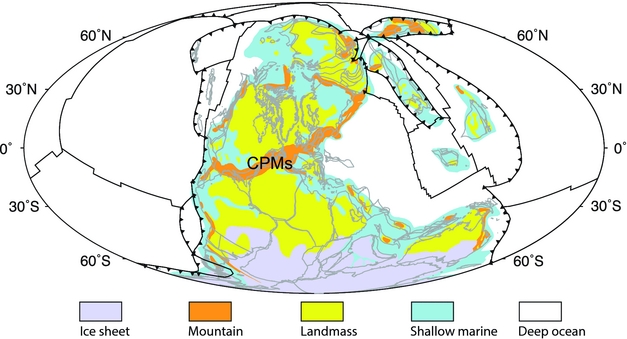
The evolution of latitudinal belts of coal samples with 50% confidence interval (Fig. 12a) may reflect the complex Phanerozoic fluctuations in the latitudinal extent of continental humid zones. The latitudinal distribution of coals with 50% confidence changes over long timescales (Figs 5, 12a), being concentrated at low latitudes during the Carboniferous period, middle latitudes during Permian and Triassic times, high latitudes during Jurassic – Early Palaeogene times, before returning to middle latitudes during Middle Palaeogene–modern times. The distribution during the Devonian period is unlikely to be reliable due to a lack of data samples (Figs 1, 2). The Carboniferous period is significantly different from post-Palaeozoic times (Fig. 12a). Abundant coal samples were accumulated in tropical regions (~0–25°N and S) during the Carboniferous period, while they were mostly deposited at middle or high latitudes during Mesozoic and Cenozoic times (Fig. 12a). This shift could indicate a climatic transition from humid to arid conditions from the Late Pennsylvanian through the Early Permian on equatorial Pangaea (Rowley et al. Reference Rowley, Raymond, Parrish, Lottes, Scotese and Ziegler1985; Ziegler, Reference Ziegler, McKerrow and Scotese1990; Parrish, Reference Parrish1993; Ziegler, Hulver & Rowley, Reference Ziegler, Hulver, Rowley and Martini1997; Tabor & Montañez, Reference Tabor and Montañez2004; Montañez et al. Reference Montañez, Tabor, Niemeier, DiMichele, Frank, Fielding and Isbell2007; Tabor et al. Reference Tabor, Montañez, Scotese, Poulsen, Mack, Fielding, Frank and Isbell2008; Tabor & Poulsen, Reference Tabor and Poulsen2008). Tabor & Poulsen (Reference Tabor and Poulsen2008) evaluated the climate factors possibly explaining this climate change, including changing continental configurations from tectonics, time-varying land–sea distribution, supercontinentality, monsoon, uplift/collapse of the Central Pangaean Mountains (CPMs) (Fig. 13), waxing and waning of ice sheets in Gondwanaland and atmospheric CO2. They suggested that the northward drift of most of Pangaea across climate zones, increasing atmospheric CO2 level and Gondwanaland deglaciation could have been the main factors controlling the low-latitude climate of Pangaea during Late Pennsylvanian – Early Permian times. The deglaciation of Gondwanaland is considered to be a possible cause of climate change over low-latitude Pangaea through its influence on large-scale atmospheric circulation (Ziegler et al. Reference Ziegler, Raymond, Geirlowski, Horrell, Rowley, Lottes and Scott1987; Perlmutter & Matthews, Reference Perlmutter, Matthews and Cross1989; Cecil, Reference Cecil1990; Miller & West, Reference Miller and West1993; Miller, McCahon & West, Reference Miller, McCahon and West1996; Soreghan, Reference Soreghan1997; Cecil et al. Reference Cecil, Dulong, West, Stamm, Wardlaw, Edgar, Cecil and Edgar2003; Perlmutter & Plotnick, Reference Perlmutter, Plotnick, Cecil and Edgar2003; Poulsen et al. Reference Poulsen, Pollard, Montañez and Rowley2007). Late Palaeozoic climate simulations suggest that the deglaciation of Gondwana and atmospheric CO2 rise could explain much of the Late Palaeozoic climate change over low-latitude Pangaea, and regional uplift/erosion of the CPMs has a secondary effect on tropical precipitation (Peyser & Poulsen, Reference Peyser and Poulsen2008). However, the change from dominantly humid palaeoclimate indicators in Pennsylvanian strata to arid and seasonal indicators in Permian strata is considered possibly related to the evolution of the CPMs (Goddéris et al. Reference Godderis, Donnadieu, Carretier, Aretz, Dera, Macouin and Regard2017).
Global palaeogeography in the Late Carboniferous from Cao et al. (Reference Cao, Zahirovic, Flament, Williams, Golonka and Müller2017) showing the location of the Central Pangaean Mountains (CPMs). Black toothed lines indicate subduction zones, and other black lines denote middle-ocean ridges and transforms. Grey outlines delineate reconstructed present-day coastlines and terranes. Mollweide projection with 0°E central meridian.

We compared our results to a recent estimate of atmospheric CO2 since the Devonian period (Foster, Royer & Lunt, Reference Foster, Royer and Lunt2017; Fig. 12d), and to additional aspects of Earth's palaeogeographic history extracted from digital palaeogeographic reconstructions (Golonka et al. Reference Golonka, Krobicki, Pajak, Giang and Zuchiewicz2006; Cao et al. Reference Cao, Zahirovic, Flament, Williams, Golonka and Müller2017; Fig. 12e–g). Atmospheric CO2 levels do not indicate significant changes at the beginning of the Permian period that would directly coincide with the poleward shift in coal distributions. The areas of tropical mountain ranges close to the equator (Fig. 12e), thought to be regions of significantly enhanced weathering rates, similarly do not record a significant change from the Late Pennsylvanian through the Early Permian (Fig. 12e). In addition, we computed Phanerozoic ice-sheet areas from palaeogeographic maps (Golonka et al. Reference Golonka, Krobicki, Pajak, Giang and Zuchiewicz2006; Cao et al. Reference Cao, Zahirovic, Flament, Williams, Golonka and Müller2017), and the results indicate that ice sheets indeed considerably reduced during the Late Pennsylvanian – Early Permian transition (Fig. 12g). Plate tectonic configurations (Golonka, Reference Golonka2007; Scotese, Reference Scotese2008; Matthews et al. Reference Matthews, Maloney, Zahirovic, Williams, Seton and Müller2016) indicate that most of Pangaea moved rapidly northward during the Late Pennsylvanian – Early Permian transition. Walker, Wilkinson & Ivany (Reference Walker, Wilkinson and Ivany2002) argued that these motions influenced patterns of shallow-marine carbonates during Phanerozoic times through a long-term decrease in areas of tropical shelf based on the palaeogeographic atlas of Scotese & Golonka (Reference Scotese and Golonka1992), although, a persistent decrease in the area of tropical shallow marine environments over the past ~400 Ma is less apparent in palaeogeographic maps of Golonka et al. (Reference Golonka, Krobicki, Pajak, Giang and Zuchiewicz2006) and Cao et al. (Reference Cao, Zahirovic, Flament, Williams, Golonka and Müller2017) (Fig. 12f). The resulting migration of tropical basins from humid climate zones associated with the Intertropical Convergence Zone into the adjacent northern subtropical zone could be attributed to long-term tropical aridification (Ziegler et al. Reference Ziegler, Hansen, Johnson, Kelly, Scotese and Van der Voo1977; Witzke, Reference Witzke, McKerrow and Scotese1990; Gibbs et al. Reference Gibbs, Rees, Kutzbach, Ziegler, Behling and Rowley2002; Rees et al. Reference Rees, Ziegler, Gibbs, Kutzbach, Behling and Rowley2002; Tabor et al. Reference Tabor, Montañez, Scotese, Poulsen, Mack, Fielding, Frank and Isbell2008).
It is important to consider some non-climatic factors that may influence the latitudinal distributions of these lithologies. Carboniferous coal-forming flora were dominated by pteridophytes with a low tolerance to groundwater fluctuations due to their shallow root system, making them less likely to form thick preserved coal seams even where favourable peat-forming conditions existed (Diessel, Reference Diessel1992). In contrast, post-Carboniferous coal measures were dominated by Gymnosperms from the Permian to the Cretaceous and angiosperms since the Triassic. They can occupy a wider range of latitudes due to their greater tolerance to groundwater fluctuations and adaptability in more fully marginal peat-forming conditions (Diessel, Reference Diessel1992). The evolution of plant groups through space and time could contribute to the changing distributions of coal deposits through time, especially its significant poleward shift in the Early Permian. Additionally, a further contributor to the Carboniferous low-latitude peak in coal distribution could be the relatively rare occurrence of extensive foreland-basin systems within the tropics during Pangaea assembly, ideal for the formation and preservation of coal (Nelsen et al. Reference Nelsen, DiMichele, Peters and Boyce2016). In summary, the major poleward shift in coal distributions beginning in the Early Permian is likely to be driven by a combination of processes, resulting from the interplay of tectonics, deglaciation, evolution of plants and palaeoclimate.
The changing latitudinal belts of evaporites with 50% confidence (Fig. 12b) indicate the evolution of low-latitudinal arid zones over time, but the fluctuations are subtle relative to other indicators. During the Early Palaeogene, they underwent a relatively rapid shift away from the equator, contemporaneous with climate-driven shifts in coals and glacial deposits. In older times, the origins of changes are less clear (Fig. 12b). Ancient marine evaporite formation is not only related to dry climate but also tectonic setting (Warren, Reference Warren2010). For instance, during the Early Devonian, many evaporites occurred in the northern margins of tropical Laurentia and low-latitude Siberia (Fig. 1), which could explain the equatorial distribution of evaporites during the time (Fig. 12b). The latitudinal belt of evaporites shifts poleward to mean latitudes of ~25°N and S during Middle Devonian – Early Carboniferous time (Fig. 12b). This could be mostly due to evaporites accumulating in the southern, western or eastern margins of Laurentia during the Middle Devonian – Early Carboniferous time (Fig. 1). From the assembly of Pangaea in the Late Carboniferous until the Middle Triassic (Ziegler et al. Reference Ziegler, Scotese, McKerrow, Johnson and Bambach1979), abundant evaporites occur in the western and eastern margins of low-latitude Pangaea (Fig. 1). Starting from the Late Triassic (~240 Ma) the pattern of rift basins formed during Pangaea break-up (notably the Atlantic margins and the Gulf of Mexico) will have exerted an additional control on evaporite distributions (Fig. 1).
Atmospheric CO2 is thought to be a primary driver of both ice-sheet and climate variability (Montañez & Poulsen, Reference Montañez and Poulsen2013; Lowry et al. Reference Lowry, Poulsen, Horton, Torsvik and Pollard2014; Foster, Royer & Lunt, Reference Foster, Royer and Lunt2017), and solar luminosity secondarily influences Palaeozoic glaciation (Lowry et al. Reference Lowry, Poulsen, Horton, Torsvik and Pollard2014). Mountain uplift enhances silicate rock weathering, resulting in a decrease in atmospheric CO2 concentrations (Kump & Arthur, Reference Kump, Arthur and Ruddiman1997; Berner, Reference Berner2004; Montañez & Poulsen, Reference Montañez and Poulsen2013; Foster, Royer & Lunt, Reference Foster, Royer and Lunt2017). The latitudinal distribution patterns of glacial deposits reported in this study (Fig. 12c) record three major Phanerozoic glacial periods, during Carboniferous–Permian, Late Jurassic – early Cretaceous and Cenozoic times (Frakes, Francis & Syktus, Reference Frakes, Francis and Syktus1992). The late Palaeozoic icehouse is the longest-lived ice age of the Phanerozoic (Montañez & Poulsen, Reference Montañez and Poulsen2013). Ice sheets were abundant over the South Pole during this period. This ice age corresponds to intense mountain uplift around tropical Pangaea (Fig. 12e) which could have contributed to late Palaeozoic cooling through enhanced silicate weathering (Kump et al. Reference Kump, Arthur, Patzkowsky, Gibbs, Pinkus and Sheehan1999; Goddeŕis et al. Reference Godderis, Donnadieu, Carretier, Aretz, Dera, Macouin and Regard2017). The high temperature gradients during the time, derived from the comprehensive global-scale compilation of lithologies (Boucot & Gray, Reference Boucot and Gray2001; Boucot, Chen & Scotese, Reference Boucot, Chen and Scotese2013), also indicate a cooling (Fig. 12h). The Cenozoic glaciation corresponds to remarkable topographic uplift (Fig. 12e) of the Himalaya – Tibetan Plateau (Molnar & England, Reference Molnar and England1990) contributing to atmospheric CO2 decrease through enhanced silicate weathering and resulting high temperature gradients (Fig. 12h). Therefore, our results suggest that mountain uplift could have been an important factor in the two major ice ages in late Palaeozoic and Cenozoic times through decreased atmospheric CO2 and enhanced temperature gradients. Yet, other factors including organic carbon burial and outgassing through volcanism and metamorphism (e.g. Pearson & Palmer, Reference Pearson and Palmer2000) might also contribute to the drawdown of atmospheric CO2.
5.c. Workflow limitations
The presented workflow uses a 5°×5° grid of Earth's surface to bin lithology data points. By resampling the data points, we removed the spatial sampling bias. However, latitude strips at or near the equator have larger areas than the polar ones (see fig. 1 in Vilhena & Smith, Reference Vilhena and Smith2013), which leads to over-binning in high-latitude strips. Ideally, an equal-area gridding scheme would be created to correct spatial sampling bias in the dataset (Vilhena & Smith, Reference Vilhena and Smith2013), and this could be considered in future work. However, we used the simpler 5° × 5° binning so that our results are comparable to the previous study of Ziegler et al. (Reference Ziegler, Eshel, McAllister Rees, Rothfus, Rowley and Sunderlin2003).
There is also a temporal sampling bias in the workflow. The reconstruction ages used to construct the climatically sensitive lithologic data to ancient geographic locations represent discrete time periods of several millions of years. Because the reconstructed palaeogeographic locations of the lithologic data points change within the time range for which their age is assigned in the source data, sample locations are not truly defined by one point palaeolocation, and could be represented by an average location over a given time period in future work. Providing a continuous representation of palaeolatitudinal distribution patterns indicated from palaeoclimate lithologic data remains an important challenge. The temporal resolution in this study does not allow us to capture some short-term fluctuations which may be interpreted from more detailed records (e.g. Horton, Poulsen & Pollard, Reference Horton, Poulsen and Pollard2010; Montañez et al. Reference Montañez, McElwain, Poulsen, White, DiMichele, Wilson, Griggs and Hren2016). For instance, our workflow considers the time interval 290–252 Ma during the Permian period as a single stage, and cannot reflect the fluctuations indicated from atmospheric CO2 level during that time (Fig. 12a, d). Higher temporal resolution would make it possible to refine climate reconstructions.
A further improvement to our analysis could be to use palaeogeographic maps rather than continental polygons to correct for the bias due to the uneven distribution of areas through time over the lithologic data. Such maps have the potential to provide a clearer definition of which areas within the continental polygons used here are likely to host certain types of lithologies associated specifically with shallow marine or terrestrial environments. However, such palaeogeographic maps (e.g. Ronov, Khain & Seslavinsky, Reference Ronov, Khain and Seslavinsky1984); Ronov, Khain & Balukhovsky, Reference Ronov, Khain and Balukhovsky1989); Scotese, Reference Scotese2001, Reference Scotese2004; Golonka et al. Reference Golonka, Krobicki, Pajak, Giang and Zuchiewicz2006; Blakey, Reference Blakey, Fielding, Frank and Isbell2008; Cao et al. Reference Cao, Zahirovic, Flament, Williams, Golonka and Müller2017) are more interpretive than continental polygons and typically do not use divisions of the geological timescale that are exactly consistent either with each other or with the time range definitions of the lithologic data considered here, and remains an outstanding problem in terms of how to obtain palaeogeographic maps and lithologies at the same temporal resolution.
6. Conclusions
This study provides a framework to investigate the shifting climatic zones through deep geological time by using plate reconstructions, a comprehensive database and new data analysis approaches. We quantified the palaeolatitudinal zonal patterns of climate-lithologic deposits of coals, evaporites and glacial deposits since the Devonian, with corrections for sampling- and area-biases, and used statistical methods (SiZer and HDR) to obtain probability density functions and estimate high-probability latitudinal belts. The sensitivity test of the latitudinal distributions of climate-sensitive lithologic deposits on uneven distribution of continental areas through time indicates that these climate indicators are sensitive to the correction of continental areas, and that the distribution of coals is more sensitive than evaporites and glacial deposits to this correction, particularly in Middle Devonian, Carboniferous, Early and Middle Triassic, Jurassic, Cretaceous and Early Palaeogene times. The latitudinal distributions of these lithologic indicators do not show strong sensitivity to the reconstruction model.
The distribution of coal palaeolatitudes herein, with higher temporal resolution than previous studies, shifted to significantly higher latitudes at the beginning of the Permian, contrasting with the previous suggestion that the shift started in the Carboniferous (Diessel, Reference Diessel1992). The changing distribution of coals over the period from the Permian to the present also cannot be considered to have been constant as proposed by Ziegler et al. (Reference Ziegler, Eshel, McAllister Rees, Rothfus, Rowley and Sunderlin2003). Our results indicate a clearly bimodal distribution of evaporites over the past ~400 Ma, except for the Early Devonian, Early Carboniferous, the earliest Permian and Middle and Late Jurassic (Fig. 6f). This suggests that the previously proposed bimodal or unimodal evaporite patterns could have alternated over geological times. The distribution of glacial deposits is consistent with previous interpretations of the main icehouse and greenhouse periods during the last ~400 Ma.
We considered some of the main factors controlling the latitudinal distributions of the lithologic deposits over time. There is no single factor that dominates the changing distributions from the Early Devonian to the present. As many previous studies have noted, tectonic factors associated with Pangaea assembly and break-up and the waxing and waning of ice sheets in Gondwanaland could have been significant factors influencing the distributions of the lithologies, including the extent of tropical continental humid zones from the Late Pennsylvanian through the Early Permian. The evolution of plant groups through space and time has influenced coal distributions, especially in a significant poleward shift during the Early Permian due to the rise of Gymnosperms. Due to these many factors, care should be taken when using the latitudinal distribution of these lithologies to constrain both past global climate and the past positions of continents.
Acknowledgements
This work is supported by Australian Research Council (ARC) grants IH130200012 (R.D.M., S.Z., S.W.) and ARC DE160101020 (N.F.). W. Cao was also supported by a University of Sydney International Scholarship (USydIS). This work also benefited from support of the Alfred P. Sloan Foundation (G-2017-9997) and the Deep Carbon Observatory (DCO). We thank John Cannon and Michael Chin for help with GPlates and pyGPlates, and Sally Cripps, Rohitash Chandra, Rob Hyndman, Stephen Marron and Maelis Arnould for assistance with programming.
Supplementary material
To view supplementary material for this article, please visit https://doi.org/10.1017/S0016756818000110
Appendix: Software availability
SiZer analysis is performed in MatLab using the ‘Smoothing’ package (Chaudhuri & Marron, Reference Chaudhuri and Marron1999) available at http://www.stat.unc.edu/faculty/marron/marron_software.html. SiZer can also be found in the package ‘feature’ (version 1.2.13) in ‘R’ statistical software (version 3.3.2). HDR from Hyndman (Reference Hyndman1996) is performed using the ‘hdrcde’ package (version 3.1) in ‘R’ statistical software (version 3.3.2). The HEALPix method is conducted using the library ‘healpy’ (version 1.10.3) in Python 2.0 and its documentation is available at http://healpy.readthedocs.io/en/latest/index.html.