


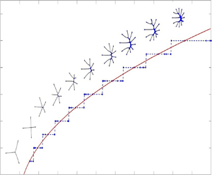



1. Introduction
Saffman–Taylor instabilities (Saffman & Taylor Reference Saffman and Taylor1958) occur when a less viscous fluid is injected into a more viscous fluid confined in a fixed narrow gap between two parallel plates (Hele-Shaw cell). During injection, the inner less viscous fluid displaces the outer viscous fluid and the interface separating the two fluids exhibits fingering patterns (Langer Reference Langer1989; Cummins, Fourtune & Rabaud Reference Cummins, Fourtune and Rabaud1993). Through repeated tip-splitting events, new fingers develop and the proliferation of fingers leads to dense branching morphologies as the system is driven out of equilibrium (Chuoke, van Meurs & van der Poel Reference Chuoke, van Meurs and van der Poel1959; McLean & Saffman Reference McLean and Saffman1981; Park, Gorell & Homsy Reference Park, Gorell and Homsy1984; Ben-Jacob et al. Reference Ben-Jacob, Deutscher, Garik, Goldenfeld and Lareah1986; Praud & Swinney Reference Praud and Swinney2005; Li, Lowengrub & Leo Reference Li, Lowengrub and Leo2007). Viscous fingering is considered a paradigm for a variety of pattern forming phenomena such as bacterial colony growth and snowflake formation as the physical mechanisms and mathematical structure are similar (Langer Reference Langer1980, Reference Langer1989; Ben-Jacob & Garik Reference Ben-Jacob and Garik1990).
One variant of the conventional Hele-Shaw set-up that provides another way to produce viscous fingering patterns is the so-called lifting plate problem (Shelley, Tian & Wlodarski Reference Shelley, Tian and Wlodarski1997; Chen, Chen & Miranda Reference Chen, Chen and Miranda2005; Tatulchenkov & Cebers Reference Tatulchenkov and Cebers2008; Sinha, Dutta & Tarafdar Reference Sinha, Dutta and Tarafdar2008; Sinha & Tarafdar Reference Sinha and Tarafdar2009; Dias & Miranda Reference Dias and Miranda2010; Nase, Derks & Lindner Reference Nase, Derks and Lindner2011). In the lifting plate problem, the top plate in a Hele-Shaw cell is lifted perpendicularly at a prescribed speed and the bottom plate remains at rest. This set-up has been used to study adhesion-related problems such as debonding (Francis & Horn Reference Francis and Horn2001; Derks et al. Reference Derks, Lindner, Creton and Bonn2003; Poivet et al. Reference Poivet, Nallet, Gay and Fabre2003; Ben Amar & Bonn Reference Ben Amar and Bonn2005) and the associated probe tack test (Zosel Reference Zosel1985; Lakrout, Sergot & Creton Reference Lakrout, Sergot and Creton1999).
In the lifting plate problem, the gap  $b(t)$ between the two plates is increasing in time but uniform in space. As the plate is lifted, an inner viscous fluid rushes inward between the two plates and increases in the
 $z$-direction to preserve volume. An outer less viscous fluid (usually air) invades the more viscous fluid and generates fingering patterns. The patterns are visually similar to those in the classical radial Hele-Shaw problem, but the driving physics is different in the sense that the flow in this problem is extensional (e.g. free-surface instabilities seen in McKinley & Sridhar (Reference McKinley and Sridhar2002)). Viscous fingering patterns can also be observed using a Hele-Shaw cell where only one edge of the plate is lifted, which makes the gap width a function of time and space (Zhang et al. Reference Zhang, Louis, Pla and Guinea1998; Dias & Miranda Reference Dias and Miranda2013b).
To characterize pattern formation in the lifting plate problem, the number of fingers has been studied using experiments and theory using Darcy's law as an approximation. Theoretical studies (Ben Amar & Bonn Reference Ben Amar and Bonn2005; Lindner, Derks & Shelley Reference Lindner, Derks and Shelley2005; Sinha et al. Reference Sinha, Dutta and Tarafdar2008; Nase et al. Reference Nase, Derks and Lindner2011; Dias & Miranda Reference Dias and Miranda2013a) show that the number of fingers is controlled by a dimensionless surface tension. However, experiments using constant rates of increasing gap widths suggest that the total number of fingers is not only dependent on the dimensionless surface tension but also on the confinement, or aspect ratio of the fluid,  $C_0={R_0}/{b_0}$, where
 $R_0$ is the initial radius of the liquid and
 $b_0$ is the initial gap width (Nase et al. Reference Nase, Derks and Lindner2011); see also figure 2 in § 3 where experimental data is plotted together with the results from linear theory and nonlinear simulations. In general, increasing
 $C_0$ results in an increased number of fingers. In these studies, the rate of increase in the gap width over time is limited, e.g. constant rates of increase. Accordingly, the viscous fingering instability is transient and eventually the interface shrinks as a circle. Interfacial dynamics in the regime where the gap width increases more rapidly in time, which could lead to non-circular vanishing limiting shapes, has been much less explored.
In this paper, we investigate regimes in which the gap width increases rapidly in time. Motivated by linear theory (Dias & Miranda Reference Dias and Miranda2010; Zhao et al. Reference Zhao, Li, Yin, Belmonte, Lowengrub and Li2018), we consider gaps of the form  $b_{\mathcal {C}}(t)=(1-({7}/{2})\tau \mathcal {C} t)^{-{2}/{7}}$, where
 $\tau$ is the surface tension and
 $\mathcal {C}$ is a coefficient. This temporal variation in gap width has also been used to control the interface in miscible confined flows without surface tension (Chen et al. Reference Chen, Huang, Wang and Miranda2010). Here, the gap width increases much more rapidly than
 $b(t)\sim t$ or even
 $b(t)\sim \textrm {e}^t$ and actually tends to infinity at a finite time, dictated by the surface tension and the coefficient
 $\mathcal {C}$. If
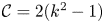 $\mathcal {C}=2(k^2-1)$, with
 $k$ being the perturbation wavenumber, a
 $k$-mode perturbation evolves self-similarly (e.g. perturbation size relative to underlying shrinking circle is invariant). Alternatively, if
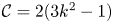 $\mathcal {C}=2(3k^2-1)$ then mode
 $k$ is the fastest growing mode. In both cases, this leads to non-circular vanishing limiting shapes at least at the level of linear theory. Predictions of the nonlinear dynamics and the emergent interface patterns in the nonlinear regime are very difficult because of non-locality, strong nonlinearity and rapid evolution. Consequently, until this work the effect of nonlinearity in this special, shrinking regime had not yet been explored.
Here, we use a recently developed spectrally accurate boundary integral method with space–time rescaling (Zhao et al. Reference Zhao, Li, Yin, Belmonte, Lowengrub and Li2018) that enables the accurate simulation of nonlinear interface dynamics in the fast shrinking regime for the first time. In particular, the interface is mapped back to its initial size, and time is rescaled such that the speed of the interface in the new frame is prescribed and is slower than the dynamics in the original frame. Thus, a fixed time step in the rescaled frame corresponds to a time step in the original frame that is adaptively and rapidly decreased in time. Together, these features enable us to accurately simulate the fully nonlinear dynamics of the interface at extraordinarily small interface sizes and obtain nonlinear, limiting shapes that have not been previously reported. Other forms of space–time rescaling are also used to study the behaviour of bubble extinction in a Hele-Shaw flow (Dallaston & McCue Reference Dallaston and McCue2013, Reference Dallaston and McCue2016).
To validate our methods, we compare with experiments from Nase et al. (Reference Nase, Derks and Lindner2011) where the linear gap  $b(t)\sim t$ is used. Our numerical predictions for the number of fingers are in quantitative agreement with the experiments when the confinement number
 $C_0$ is large. This is in contrast with the results of linear theory, which predict fewer fingers and provide a better match to the experimental results at smaller
 $C_0$ (Nase et al. Reference Nase, Derks and Lindner2011; Dias & Miranda Reference Dias and Miranda2013a). This illustrates the importance of accounting for nonlinear interactions.
In the special shrinking regime, where  $b(t)=b_{\mathcal {C}}$ is used, our numerical simulations reveal the existence of strikingly thin,
 $k$-fold dominant, limiting interfacial shapes. This suggests that these interfaces do not shrink as circles but rather as novel one-dimensional, web-like networks. Although we do not find evidence of self-similar dynamics in the nonlinear regime, we do find that there is mode selection. We construct a morphology diagram for pattern selection that relates the dominant mode
 $k$ of the vanishing, limiting interface and the control parameter
 $\mathcal {C}$.
This paper is organized as follows. In § 2, we present the governing equations, the linear stability analysis and the boundary method used to simulate the nonlinear system. In § 3, we present numerical results and in § 4, we give conclusions and discuss future work. In the appendices, we show that if we slightly modify the dynamics of the gap width in time (by making it slightly larger than reported in the experiment), then quantitative agreement between the simulations and experiments can be achieved at small confinement numbers and surface tensions when the gap width increases linearly in time. Also in the appendices, we present additional numerical results in the special-shrinking regime. Finally, in the appendices, we provide a comparison between the nonlinear simulations and new experiments for shrinking interfaces using a gap width that increases nonlinearly in time.
2. Governing equations
We consider a radial Hele-Shaw cell with a time-dependent gap  $\tilde {b}(\tilde {t})$, see figure 1 for a schematic. The upper plate is lifted uniformly in space while the lower plate is stationary. The domain
 $\tilde {\varOmega }(\tilde {t})$ denotes the region containing the viscous fluid (e.g. oil) and
 $\partial \tilde {\varOmega }(\tilde {t})$ denotes its interface. A less viscous fluid (e.g. air) is contained in the exterior of
 $\tilde {\varOmega }(\tilde {t})$. Here, the tildes denote dimensional variables. The non-dimensional system, which we analyse and solve numerically, is given below.
Schematic for the lifting plate Hele-Shaw problem. The region  $\varOmega (t)$ contains oil with viscosity
 $\mu$. The region exterior to
 $\varOmega (t)$ contains air. Here
 $b(t)$ is the time dependent gap width. The normal
 $\boldsymbol {n}$ to the interface
 $\partial \varOmega (t)$ points into
 $\varOmega (t)$. Here
 $R$ denotes the equivalent radius (radius of a circle with the same enclosed area).

2.1. Governing equations
Following previous studies (Ben Amar & Bonn Reference Ben Amar and Bonn2005; Lindner et al. Reference Lindner, Derks and Shelley2005; Sinha et al. Reference Sinha, Dutta and Tarafdar2008; Nase et al. Reference Nase, Derks and Lindner2011; Dias & Miranda Reference Dias and Miranda2013a), we assume that the motion of the fluid is governed by Darcy's law, which is a two-dimensional approximation of the Navier–Stokes system obtained by averaging the equations over the narrow gap between the plates. Following Lamb (Reference Lamb1932), He & Belmonte (Reference He and Belmonte2011) and Anjos, Dias & Miranda (Reference Anjos, Dias and Miranda2017), the two-dimensional approximation holds when  $\mathcal {E}={\tilde {b}(\tilde {t})}/{\tilde {R}(\tilde {t})}\ll 1$ and Reynolds number
 $Re=({\rho \tilde {b}(\tilde {t}) \dot {\tilde {b}}(\tilde {t})})/{12 \mu }\ll 1$, where
 $\tilde {R}$ is the equivalent radius of the fluid drop,
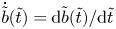 $\dot {\tilde {b}}(\tilde {t})={\textrm {d}\tilde {b}(\tilde {t})}/{\textrm {d}\tilde {t}}$ is the lifting speed of the upper plate,
 $\rho$ is the density of the fluid and
 $\mu$ is the viscosity of the fluid. The equations are
 \begin{equation} \tilde{\boldsymbol{u}}={-}\frac{\tilde{b}^2(\tilde{t})}{12\mu}\tilde{\boldsymbol{\nabla}} \tilde{P} \quad \text{in} \quad\tilde{\varOmega}(\tilde{t}),\end{equation}
where  $\tilde {\boldsymbol {u}}$ is the velocity and
 $\tilde {P}$ is the pressure.
From volume conservation, we obtain the gap-averaged incompressibility condition as
 \begin{equation} \tilde{\boldsymbol{\nabla}}\boldsymbol{\cdot}\tilde{\boldsymbol{u}}={-}\frac{\dot{\tilde{b}}(\tilde{t})}{\tilde{b}(\tilde{t})}\quad \text{in} \ \tilde{\varOmega}(\tilde{t}). \end{equation}
The pressure jump  $[\tilde {P}]$ across the interface is given by the Laplace–Young condition, which is the product of surface tension
 $\sigma$ and the curvature
 $\mathcal {K}$ (Park & Homsy Reference Park and Homsy1984; Dias & Miranda Reference Dias and Miranda2013a; Anjos & Miranda Reference Anjos and Miranda2014), as follows:
 \begin{equation} [\tilde{P}]=\tilde{P}|_{\partial\varOmega^+}-\tilde{P}|_{\partial\varOmega^-}=\sigma\mathcal{K} \quad \text{on}\quad \partial\tilde{\varOmega}(\tilde{t}), \end{equation}
where the  $+/-$ superscripts denote the limit from the exterior and interior of
 $\varOmega$, respectively. We approximate the curvature as
 $\mathcal {K}=\tilde {\kappa }+({2}/{\tilde {b}(\tilde {t})})\cos (\theta _c)$, where
 $\tilde {\kappa }$ denotes the curvature of the planar interfacial curve and
 $\theta _c$ represents the contact angle measured between the plates and the curved meniscus. The second term accounts for the curvature across the gap width, which is associated with the interface profile in the z-direction. When
 $\tilde {b}(\tilde {t})$ increases, this term decreases indicating that surface tension effects across the gap become weaker. However,
 $\tilde {\kappa }$ increases since the interface shrinks. Even though the second term varies with time, it is uniform in space if we assume
 $\theta _c$ is a constant. Thus it can be absorbed in the pressure as a redefined pressure. We use this redefined pressure in the rest of this paper. The scaled normal derivative
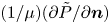 $({1}/{\mu })({\partial \tilde {P}}/{\partial \boldsymbol {n}})$ is continuous across
 $\partial \varOmega$ and the normal velocity of the interface is thus
 \begin{equation} \tilde{V}={-}\frac{\tilde{b}^2(\tilde{t})}{12\mu}\frac{\partial \tilde{P}}{\partial \boldsymbol{n}}\quad \text{on}\ \partial\tilde{\varOmega}(\tilde{t}), \end{equation}
where  $\boldsymbol {n}$ is the unit normal vector pointing into
 $\tilde {\varOmega }(\tilde {t})$.
We non-dimensionalize the system using a characteristic length  $L_0$, time
 $T={\tilde {b}_0}/{\dot {\tilde {b}}_0}$ and pressure
 $P_0=({12\mu L_0^2})/({T\tilde {b}_0^2})$, where
 $L_0$ is a characteristic size of the initial fluid domain
 $\varOmega (0)$, and
 $\tilde {b}_0$ and
 $\dot {\tilde {b}}_0$ are the initial values of
 $\tilde {b}$ and
 $\dot {\tilde {b}}$. Further, we define the non-dimensional modified pressure as
 ${P}=\tilde {P}/P_0- ({\dot {b}(t)}/{4b^3(t)})|\boldsymbol {x}|^2$, where
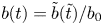 $b(t)=\tilde {b}(\tilde {t})/b_0$,
 $t=\tilde {t}/T$,
 ${\dot {b}(t)={\textrm {d}b}/{\textrm {d}t}}$ and
 $\boldsymbol {x}=\tilde {\boldsymbol {x}}/L_0$. Then, the non-dimensional version of (2.1)–(2.4) becomes
 \begin{gather} \nabla^2 {P}=0\quad \text{in}\ \varOmega, \end{gather}
 \begin{gather}{}[{P}]=\tau \kappa-\frac{\dot{b}(t)}{4b^3(t)}|\boldsymbol{x}|^2\quad \text{on}\ \partial\varOmega, \end{gather}
 \begin{gather} V={-}b^2(t)\frac{\partial{P}}{\partial \boldsymbol{n}}+\frac{\dot{b}(t)}{2b(t)}\boldsymbol{x}\boldsymbol{\cdot}\boldsymbol{n}\quad\textrm{on}\ \partial\varOmega, \end{gather}
where 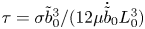 $\tau ={\sigma \tilde {b}_0^3}/({12\mu \dot {\tilde {b}}_0L_0^3})$ is a non-dimensional surface tension. Taking
 $L_0$ to be the equivalent radius of
 $\varOmega (0)$, e.g. the radius of a circle with the same enclosed area, the non-dimensional volume of the fluid is
 ${\rm \pi}$ since the initial non-dimensional gap is
 $b(0)=1$.
2.2. Linear theory
In this section, we briefly review the linear stability analysis in Shelley et al. (Reference Shelley, Tian and Wlodarski1997) and Zhao et al. (Reference Zhao, Li, Yin, Belmonte, Lowengrub and Li2018). We consider the interface to be a slightly perturbed circle,
 \begin{equation} r(\alpha,t)=R(t)+\epsilon \delta(t)\cos(k\alpha), \end{equation}
where  $\epsilon$
 $\ll 1$, the perturbation mode
 $k\geq 2$ is an integer,
 $\alpha \in [0,2{\rm \pi} ]$ is the polar angle and
 $\delta (t)$ is the amplitude of the perturbation. The shape factor
 $({\delta }/{R})(t)={\delta (t)}/{R(t)}$ can be used to characterize the size of the perturbation relative to the underlying circle (Mullins & Sekerka Reference Mullins and Sekerka1963). Then, it can be shown that the shape factor evolves according to
 \begin{equation} \left(\frac{\delta}{R}\right)^{{-}1}\frac{\textrm{d}}{\textrm{d}t}\left(\frac{\delta}{R}\right)=\frac{\dot{b}k}{2b}- \tau\frac{b^2(k^3-k)}{R^3}. \end{equation}
Using the relationship 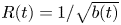 $R(t)={1}/{\sqrt {b(t)}}$, which arises from volume conservation at the level of linear theory, the shape factor grows only when
 \begin{equation} \dot{b}(t)>2\tau (k^2-1)b^{9/2}(t). \end{equation}
This indicates that the band of modes satisfying 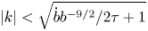 ${|k|<\sqrt {{\dot {b}b^{-9/2}}/{2\tau }+1}}$ are unstable and the interface can develop fingering patterns. Note that in the special cases that
 $\dot {b}=1$, or even
 $\dot {b}=b$, all modes
 $|k|>1$ become stable in the long time limit. This occurs because
 ${\dot {b}b^{-9/2}}\to 0$ as
 $t\to \infty$. On the other hand, if we consider much faster rates of gap increase,
 \begin{equation} b(t)=\left(1-\tfrac{7}{2}\tau \mathcal{C}t\right)^{-{2}/{7}} , \end{equation}
where  $\mathcal {C}$ is a constant, then the band of unstable modes is fixed in time and depends on
 $\mathcal {C}$ where
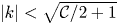 ${|k|<\sqrt {\mathcal {C}/2+1}}$. Note this gap tends to infinity at the finite time
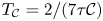 $T_{\mathcal {C}}=2/(7\tau \mathcal {C})$.
We find the fastest growing mode  $k_{max}$ by setting
 \begin{equation} \frac{\textrm{d}}{\textrm{d}k}\left[\left(\frac{\delta }{R}\right)^{{-}1}\frac{\textrm{d}}{\textrm{d}t}\left(\frac{\delta}{R}\right) \right]=0 \end{equation}
and solving for  $k_{max}$. The maximum perturbation mode
 $k^*$ has the largest magnitude relative to its initial value. We get
 $k^*$ by solving
 \begin{equation} \frac{\textrm{d}}{\textrm{d}k}\left(\left(\frac{\delta}{R}\right)_0^{{-}1}\boldsymbol{\cdot}\left(\frac{\delta}{R}\right)\right)=0, \end{equation}
where
 \begin{equation} \frac{\delta}{R}(t)=\left(\frac{\delta}{R}\right)_0b^{{k}/{2}}(t)\exp\left({\tau (k-k^3)\int_0^tb^{7/2}(s)\,\textrm{d}s}\right) \end{equation}
and  $({\delta }/{R})_0$ is the initial perturbation. Thus, mode
 $k^*$ is given by
 \begin{equation} k^*=\sqrt{\frac{\ln{b(t)}}{\displaystyle 6\tau \int_0^t b^{7/2}(s)\,\textrm{d}s}+\frac{1}{3}}. \end{equation}
When  $({\delta }/{R})_0$ is independent of
 $k$, then
 $k^*$ corresponds to the mode with the largest amplitude. When
 $({\delta }/{R})_0$ depends on
 $k$, such as the exponential decay in (3.1), the mode with largest amplitude can be determined by solving
 $({\textrm {d}}/{\textrm {d}k})({\delta }/{R})=0$. Referring to this mode as
 $\tilde {k}^*$, we obtain
 \begin{equation} \tilde{k}^*=\sqrt{\frac{\ln{b(t)-2\beta}}{\displaystyle 6\tau \int_0^t b^{7/2}(s)\,\textrm{d}s}+\frac{1}{3}}, \end{equation}
where  $\beta$ is the decay rate of initial perturbation with respect to
 $k$. Comparing the predictions from
 $k_{max}$,
 $k^*$ and
 $\tilde {k}^*$ with experimental observations for the number of fingers, we find that at early times the number of fingers predicted from
 $k^*$ is more consistent with the experimental results. This suggests that the largest initial perturbation modes have nearly uniform magnitudes. At later times, both
 $k^*$ and
 $\tilde {k}^*$ behave similarly, decay in time and are more consistent with experimental results than
 $k_{max}$.
Note that because the growth rate of the shape factor depends on time,  $k^*$ need not be equal to
 $k_{max}$. Further, these have been used to estimate the number of fingers (Nase et al. Reference Nase, Derks and Lindner2011; Dias & Miranda Reference Dias and Miranda2013a).
When the special gap dynamics in (2.11) is used, the fastest growing mode  $k_{max}$ can be prescribed by taking
 $\mathcal {C}=2(3k_{max}^2-1)$. Under this gap dynamics, the mode
 $k_{max}$ will remain the fastest growing at all times so that
 $k_{max}=k^*$ and the shape factor is
 \begin{equation} \frac{\delta(t)}{R(t)}= \frac{\delta(0)}{R(0)}b(t)^{{k_{max}^3}/({3k^2_{max}-1})} =\frac{\delta(0)}{R(0)}R(t)^{-({2k_{max}^3}/({3k^2_{max}-1}))}, \end{equation}
which diverges as  $t\to T_C$. Alternatively, if
 $\mathcal {C}=2(\bar {k}^2-1)$, then the shape factor of mode
 $\bar {k}$ does not change in time. In other words, under linear theory, a
 $\bar {k}$-mode perturbation of the interface would evolve self-similarly. Both of these conditions suggest that in the special gap regime, there may be mode selection and that perturbations may persist (and even grow) as the fluid domain and interface shrinks.
2.3. Numerical method
Because of the strong nonlinearity and non-locality of the lifting plate equations, numerical methods are needed to characterize the nonlinear dynamics. However, the simulations are very challenging because of severe time and space step restrictions introduced by the rapid evolution and shrinking of the interface. To overcome these numerical issues, we have developed a rescaled boundary integral scheme (Zhao et al. Reference Zhao, Li, Yin, Belmonte, Lowengrub and Li2018); the method is briefly described here. The idea is to map the original time and space  $({\boldsymbol {x}},t)$ into new coordinates
 $(\bar {\boldsymbol {x}},\bar {t})$ such that the interface can evolve at an arbitrary speed in the new rescaled frame (see also Li et al. Reference Li, Lowengrub and Leo2007; Zhao et al. Reference Zhao, Belmonte, Li, Li and Lowengrub2016, Reference Zhao, Yin, Lowengrub and Li2017). Introduce a new frame
 $(\bar {\boldsymbol {x}},\bar {t})$ such that
 \begin{gather} \boldsymbol{x}=\bar{R}(\bar{t})\bar{\boldsymbol{x}}(\bar{t},\alpha), \end{gather}
 \begin{gather} \bar{t}=\int_{0}^t \frac{1}{\rho(t')}\,\textrm{d}t', \end{gather}
where the space scaling  $\bar {R}(\bar {t})$ captures the size of the interface,
 $\bar {\boldsymbol {x}}$ is the position vector of the scaled interface and
 $\alpha$ parameterizes the interface. The space scaling function maps the interface to its original size and the time scaling function
 $\rho (t)=\bar {\rho }(\bar {t})$ maps the original time
 $t$ to the new time
 $\bar {t}$, which has to be positive and continuous. If
 $\rho (t)<1$, then the evolution in the rescaled frame is slower than that in the original frame. Using mass conversation and requiring the area enclosed by the interface to be fixed in the new frame, we obtain the normal velocity in the new frame
 \begin{equation} \bar{V}= \frac{\bar{\rho}}{\bar{R}}{V}(t). \end{equation}
Representing the pressure  $P$ as a double layer potential, with dipole density
 $\bar {\gamma }$, (2.5) and (2.6) can be written as the following Fredholm integral equation of the second kind:
 \begin{equation} \bar{\gamma}(\bar{\boldsymbol{x}})+\frac{1}{\rm \pi}\int_{\partial\bar{\varOmega}(\bar{t})}\bar{\gamma}(\bar{\boldsymbol{x}}')\left[\frac{\partial \ln|\bar{\boldsymbol{x}}-\bar{\boldsymbol{x}}'|}{\partial \boldsymbol{n}(\bar{\boldsymbol{x}}')}+\bar{R}(\bar{t})\right]d\bar{s}(\bar{\boldsymbol{x}}')=2\tau \bar{\kappa}-\frac{\dot{b}(t(\bar{t}))}{2b^3(t(\bar{t}))}\bar{R}^{3}|\bar{\boldsymbol{x}}|^2. \end{equation}
Once  $\bar {\gamma }$ is determined, the normal velocity in the new frame
 $\bar {V}$ can be computed as
 \begin{equation} \bar{V}(\bar{\boldsymbol{x}})={-}\frac{b^2(t(\bar{t}))\bar{\rho}}{2{\rm \pi} \bar{R}^{3}}\int_{\partial\bar{\varOmega}}\bar{\gamma}_{\bar{s}}\frac{(\bar{\boldsymbol{x}}'-\bar{\boldsymbol{x}})^{{\perp}}\boldsymbol{\cdot}{\boldsymbol{n}}(\bar{s})}{|\bar{\boldsymbol{x}}'-\bar{\boldsymbol{x}}|^2}\,\textrm{d}\bar{s}', \end{equation}
where  $\bar {\boldsymbol {x}}^{\perp }=(\bar {x}_2,-\bar {x}_1)$ and the interface evolution in the scaled frame is
 \begin{equation} \frac{\textrm{d}\bar{\boldsymbol{x}}(\bar{t},\alpha)}{\textrm{d}\bar{t}}\boldsymbol{\cdot} \boldsymbol{n}=\bar{V}(\bar{t},\alpha). \end{equation}
Here, we take the time scaling  $\rho (t)\propto 1/\dot {b}$ so that in the rescaled frame, the gap increases linearly in time, e.g.
 $b(\bar {t})=1+c\bar {t}$, where
 $c$ is a constant. Using a spectrally accurate discretization method in space, a second-order accurate semi-implicit scheme in time and the generalized minimum residual scheme (known as GMRES) (Saad & Schultz Reference Saad and Schultz1986) to solve the Fredholm integral equation of the second kind, the method enables us to accurately compute the dynamics to far longer times than could previously be accomplished. Further details of the numerical method, including convergence studies, can be found in Zhao et al. (Reference Zhao, Li, Yin, Belmonte, Lowengrub and Li2018).
3. Numerical results
3.1. Comparison between linear theory, nonlinear simulations and experiments
We first compare the experimental results obtained in Nase et al. (Reference Nase, Derks and Lindner2011) with the results of linear theory (Dias & Miranda Reference Dias and Miranda2013a; Zhao et al. Reference Zhao, Li, Yin, Belmonte, Lowengrub and Li2018) and nonlinear simulations. In the experiments, a drop of viscous fluid, surrounded by air, was placed in a Hele-Shaw cell and the upper plate was pulled upward at a constant rate of increase, e.g. the non-dimensional gap width  $b(t)=1+t$, where
 $t$ is the non-dimensional time. High resolution images were used to precisely determine the number of fingers over time. By varying the initial drop radius, the initial plate spacing, the rate of gap increase, and the viscosity, they systematically investigated how the number of fingers depends on the non-dimensional surface tension and confinement number (see Nase et al. (Reference Nase, Derks and Lindner2011) for details).
The results from two sets of experiments are shown in figure 2. In figure 2(a,b) the number of fingers is shown as a function of the non-dimensional time for different confinement numbers  $C_0$, as labelled. The non-dimensional surface tensions are
 $\tau =3\times 10^{-5}$ (figure 2a) and
 $\tau =9.6\times 10^{-6}$ (figure 2b). The solid and dotted curves denote the number of fingers estimated from
 $k^*$ and
 $k_{max}$, respectively, obtained from linear theory. The stars denote the results from nonlinear simulations. The number of fingers in the simulations are calculated in exactly the same way as in Nase et al. (Reference Nase, Derks and Lindner2011) (e.g. number of air fingers penetrating the viscous fluid; see appendix A, figure 8). Characteristic drop morphologies using
 $\tau =9.6\times 10^{-6}$ are shown (at the non-dimensional times
 $t=1$,
 $2$,
 $3$) in figure 2(c–h) from simulations (c–e) and experiments (f–h) with
 $C_0=120$. The agreement between the experimental and simulation morphologies is striking. In our simulation, the interface eventually evolves into a circle, see figure 3 for the morphologies of the interface. Although the final gap width is approximately 16 times the initial gap width, Darcy approximation is valid (
 $\mathcal {E}\ll 1$) throughout the evolution.
Comparison between linear theory, numerical simulations and experiments from Nase et al. (Reference Nase, Derks and Lindner2011) where the gap width is increased linearly in time. The numbers of fingers over time are shown in panels (a,b) predicted by linear theory ( $k_{max}$ dotted curves;
 $k^*$ solid curves), numerical simulations (magenta stars) and experiments with different confinement numbers
 $C_0$, ranging from
 $30$ to
 $120$ as labelled. The dashed lines are exponential fits to the numerical simulations. In panel (a) the non-dimensional surface tension is
 $\tau =3\times 10^{-5}$ while in panel (b)
 $\tau =9.6\times 10^{-6}$. In panels (c–h), the simulated interfacial morphologies (c–e) and those from experiments (f–h), with
 $\tau =9.6\times 10^{-6}$, are shown at the dimensionless times
 $t=1,2,$ and
 $3$. There is an excellent agreement between the numerical simulations and experiments. Experimental results reprinted with permission.

The simulated interfacial morphologies with  $\tau =9.6\times 10^{-6}$ are shown at the dimensionless times
 $t=0$ (blue) ,
 $1$ (red),
 $12$ (black) and
 $16$ (green).

Linear theory is not able to fully describe the dynamics of the interface. But linear theory should give an insight into the dynamics. At early stages, when the perturbation is small, linear theory agrees well with nonlinear simulations. At long times, linear theory predicts that all modes vanish. In the experiments shown in Nase et al. (Reference Nase, Derks and Lindner2011), where the gap width increases linearly in time, the experiments demonstrate that the droplets vanish as a circle (see figures 3 and 4 in Nase et al. (Reference Nase, Derks and Lindner2011)), which is consistent with linear theory. In these figures, the confinement number  $C_0=60$ while we choose to present the experimental observations with confinement number
 $C_0=120$ (figure 6 in Nase et al. (Reference Nase, Derks and Lindner2011)) as figure 2(c–h). The droplet with confinement number
 $C_0=120$ also vanishes as a circle although dynamics at late times are not presented in Nase et al. (Reference Nase, Derks and Lindner2011).
To produce the nonlinear simulation results, we took the initial shape of the drop to be a slightly perturbed circle,
 \begin{equation} r(\alpha,0)=1+\epsilon\sum_{k=k_{min}}^{k_N}\textrm{e}^{-\beta k}(a_k\cos(k\alpha)+b_k\sin(k\alpha)), \end{equation}
where each  $k$,
 $a_k$ and
 $b_k$ are chosen randomly from a uniform distribution in the interval
 $(-1,1)$ and
 $\alpha$ parameterizes the interface. Varying
 $\epsilon$,
 $\beta$ and
 $k_N$ allows us to vary the amplitude of the perturbation and its modal content. Here, we took
 $\epsilon =0.05$,
 $\beta =0.2$,
 $k_{min}=2$, and
 $k_N$ is varied between 40 and 100. Since
 $b(t)\sim t$, we do not need to rescale time to slow down the evolution and take
 $\bar {t}=t$. We use N= 4096 mesh points along the interface, the time step
 $\Delta \bar {t}=1\times 10^{-4}$ and the surface tension
 $\tau =9.6\times 10^{-6}$ and
 $3\times 10^{-5}$.
As can be seen in figure 2, the number of fingers decreases in time and the drop eventually shrinks as a circle. The experimental results depend on both the confinement number  $C_0$ and the non-dimensional surface tension
 $\tau$. At larger surface tensions (figure 2a), the effect of
 $C_0$ is more pronounced at later times while at small surface tensions (figure 2b),
 $C_0$ more significantly influences the early stages of the evolution. Generally, the larger
 $C_0$ is the more fingers that are observed.
The number of fingers predicted using  $k_{max}$ significantly underpredicts the experimental (and simulation) results while the
 $k^*$ predictions agree better with the experimental data at small
 $C_0$. The numerical simulations predict more fingers than either linear estimate, and agree best with experimental data at large
 $C_0$. This illustrates the importance of accounting for nonlinear interactions. Indeed, in Zhao et al. (Reference Zhao, Li, Yin, Belmonte, Lowengrub and Li2018), it was shown that linear theory underpredicts the amplitudes of growing modes in the lifting plate problem.
For both surface tensions, the numerical simulations, and experimental data with large  $C_0$, predict a biphasic, exponential decay of the number of fingers over time; rapid decay at early times (e.g.
 $\approx \textrm {e}^{-0.75t}$ in figure 2b) and slower decay over late times (e.g.
 $\approx \textrm {e}^{-0.26t}$ in figure 2b). The experimental data with small
 $C_0$ seem to predict a single rate of exponential decay (see appendix A, figure 9), consistent with the experimental results obtained in Ben Amar & Bonn (Reference Ben Amar and Bonn2005).
It is still not yet well understood why the confinement number influences the number of fingers. Note that the thickness  $h$ of the wetting layer on the plates scales as
 $h \sim O(\textit {Ca}^{2/3})$ where
 $\textit {Ca}=\mu \tilde {V}/\sigma$ is the Capillary number (Park & Homsy Reference Park and Homsy1984; Park et al. Reference Park, Gorell and Homsy1984; Jackson et al. Reference Jackson, Stevens, Giddings and Power2015). Estimating
 $\tilde {V}\sim (\dot {b}_0/b_0) R_0= \dot {b}_0 C_0$ from (2.2) and the definition of
 $C_0$, we obtain
 $Ca\sim \dot {b}_0 C_0$. In the experiments in Nase et al. (Reference Nase, Derks and Lindner2011), the confinement number and lifting rate are changed such that the non-dimensional surface tension
 $\tau =\sigma \tilde {b}_0^3/(12\mu \dot {\tilde {b}}_0 R_0^3)$ is fixed. This implies that
 $\dot {b}_0\sim C_0^{-3}$ and therefore
 $Ca\sim C_0^{-2}$. Thus, the wetting layer thickness
 $h\sim C_0^{-4/3}$ increases as the confinement number decreases. As a simple test of this, we modified the lifting speed to reflect the fact that more fluid may be left on the plates when the confinement number is decreased, e.g. the lifting speed of the upper plate is increased to reflect the more rapid loss of fluid to the wetting layer. The results are shown in figure 10 in appendix A and indicate that with this modification, the nonlinear simulations are better able to fit experiments with smaller confinement numbers. Although, our approach for incorporating wetting effects in the model is ad-hoc, the results correlate with observed experimental trends. To more accurately account for wetting effects, we may follow the analysis in Park & Homsy (Reference Park and Homsy1984), Dias & Miranda (Reference Dias and Miranda2013a) and Anjos & Miranda (Reference Anjos and Miranda2014), where the Laplace–Young condition can be extended to account for wetting effects. This is beyond the scope of this paper and is not the subject of current research.
When wetting effects, as well as viscous stresses, are incorporated in the modified Laplace–Young condition, the range of agreement between linear predictions, using the maximum perturbation wavenumber  $k^*$, and experiments can be extended to somewhat larger
 $C_0$. However, there is still disagreement between the two at large
 $C_0$ with weakly nonlinear theory underpredicting the number of fingers, see Dias & Miranda (Reference Dias and Miranda2013a). It is very likely that nonlinear effects also play a key role and the development of a numerical method to accurately account for nonlinearity, viscous stresses, wetting effects and fluid motion in three dimensions is a subject for future work.
3.2. Limiting dynamics in the special gap regime
We next study the interfacial dynamics in the special gap regime using  $b(t)=(1-({7}/{2})\tau \mathcal {C}t)^{-{2}/{7}}$, which diverges at the finite time
 $T_C=2/(7\tau \mathcal {C})$. Recall that in this regime, according to linear theory (e.g. see § 2.2), the fastest growing mode
 $k_{max}$ and
 $\mathcal {C}$ are related by
 $k_{max}=\sqrt {(1+\mathcal {C}/2)/3}$. Further,
 $k_{max}=k^*$, the maximum perturbation mode, and the shape factor
 $\delta /R\propto R^{-2k_{max}^3/(3*k_{max}^2-1)}$, which monotonically increases over time, and diverges at
 $t=T_C$. Because of the very rapid dynamics, an infinitesimally small time step would be required as
 $t \to T_C$ if the time were not rescaled. This would make it virtually impossible to simulate the drop dynamics in the original frame. Consequently, we rescale time to slow down the evolution and take
 $\rho (t)=c/\dot {b}(t)$ so that in the new time scale
 $\bar {t}$ we have
 $b(\bar {t})=1+c\bar {t}$. This makes it possible to study the limiting dynamics in the special gap regime.
3.2.1. Examples of drop dynamics
In figure 4, we present results using  $\mathcal {C}=52$ and surface tension
 $\tau =1\times 10^{-4}$, which makes
 $k_{max}=k^*=3$. Note that we reverse the orientation of the horizontal axis to reflect the fact that the radius
 $R$ decreases with time
 $t$. That is
 $R$ decreases from 1 as
 $t$ increases from 0. We use three different initial drop shapes (see insets in figure 4a with
 $R=1$):
 $r(\alpha ,0)=1+0.02(\cos (3\alpha )+\cos (5\alpha )+\cos (6\alpha ))$ (blue);
 $r(\alpha ,0)=1+0.02(\cos (3\alpha )+\sin (7\alpha )+\cos (15\alpha )+\sin (25\alpha ))$ (magenta); and
 $r(\alpha ,0)=1+0.02(\sin (6\alpha )+\cos (15\alpha )+\sin (25\alpha ))$ (red). Note that in the latter case, mode
 $k=3$ is not present initially. Here, we take
 $c=1/2$, and use the time step
 $\Delta \bar {t}=1\times 10^{-4}$ and
 $N=8192$ points along the interface. Using the temporal rescaling (Zhao et al. Reference Zhao, Li, Yin, Belmonte, Lowengrub and Li2018), we are able to dramatically reduce the equivalent original time step
 $\Delta t$ while the rescaled time step
 $\Delta \bar {t}$ is fixed. As a consequence, the equivalent original time step
 $\Delta t$ satisfies
 $\Delta t=({R^9}/{2\tau \mathcal {C}})\Delta \bar {t}$. When
 $R$ decreases from
 $1$ to
 $2\times 10^{-4}$ as in figure 4,
 $\Delta t$ decreases from
 $9.6\times 10^{-3}$ to
 $4.9\times 10^{-36}$. Such wide ranges of time steps are handled seamlessly using our rescaling approach.
Simulations of drop dynamics in the special gap regime with  $b_{\mathcal {C}}(t)=(1-({7}/{2})\tau \mathcal {C} t)^{-{2}/{7}}$ with
 ${\mathcal {C}=52}$ so that the fastest growing linear mode is
 $k_{max}=3$. Here
 $\tau =1\times 10^{-4}$. We reverse the orientation of the horizontal axis to reflect the fact that the radius
 $R$ decreases with time
 $t$. (a) The nonlinear shape perturbations for different initial drop shapes are plotted as functions of the equivalent drop radii, as labelled (see text for details). The drop shapes near the vanishing time
 $T_C=2/(7\tau \mathcal {C})\approx 54.9$ are shown as insets. (b) The dynamics of the drop with modes 3, 5 and 6 near the vanishing time. (c) The drop perimeters as a function of the effective drop radii as they vanish, together with linear fits near the vanishing time (slopes as labelled). The perimeters tend to a finite number as the drops vanish. (d) The fractal dimensions of the drops are shown as a function of the effective drop radii, together with drop morphologies (insets) at various stages of the evolution. These suggest that the limiting shapes have one-dimensional web-like morphologies.

The nonlinear shape factor  $\delta /R$ is plotted in figure 4(a) as a function of the effective radius
 $R(t)$ in the original frame. Here, the nonlinear shape factor is calculated by
 ${\delta }/{R}=\max _{\alpha } |{|\bar {\boldsymbol {x}}(\alpha ,t)|}/{{\bar {R}}}-1 |$, where
 $\bar {\boldsymbol {x}}$ is the position vector measured from the centroid of the shape to the interface,
 ${\bar {R}}=\sqrt {{\bar {A}}/{{\rm \pi} }}$ is the effective radius of the drop in the rescaled frame and
 $\bar {A}$ is the constant area enclosed by the interface. Unlike the predictions of linear theory, the dynamics of the nonlinear shape factors are non-monotone due to nonlinear interactions among the modes, and the shape factors even decrease at early times (larger
 $R$). In particular, when mode
 $3$ is not present initially (red curve) the shape factor decreases until the drop becomes quite small (
 $R\approx 0.1$). However, as
 $R$ continues to decrease, eventually mode 3 starts to dominate and the shape factor grows rapidly. The shape perturbations grow throughout the dynamics (see also figure 5a below), which suggests that unlike the case for an expanding bubble (Li et al. Reference Li, Lowengrub and Leo2007, Reference Li, Lowengrub, Fontana and Palffy-Muhoray2009; Zhao et al. Reference Zhao, Belmonte, Li, Li and Lowengrub2016), the evolution does not become self-similar as the drop vanishes.
Asymptotic behaviours of the drops from figure 4. (a) The nonlinear shape perturbations exhibit a biphasic power-law dependence on the effective drop radii and eventually diverge as  $R^{-1}$ for
 $R\to 0$. (b) The maximum curvature of the drop also diverges as
 $R^{-1}$ for
 $R\to 0$. (c) The minimum neck width of the filaments tends to zero as
 $R^2$ for
 $R\to 0$.

The insets in figure 4(a) show the initial drop morphologies ( $R=1$, top) and the final drop morphologies (
 $R$ as labelled, bottom) in the rescaled frame (the full dynamics can be found in appendix B figure 11) . Generally, the final morphologies are seen to have a 3-fold symmetric, one-dimensional, web-like network structure although the shapes are somewhat different as the drops vanish. The late time (small
 $R$) evolution in the original frame is plotted in figure 4(b), which shows the morphologies of the drop with initial condition containing modes
 $3$,
 $5$ and
 $6$ (blue drop in figure 4a). The drop dynamics in the rescaled frame can be found in appendix B (figure 12a). As the drop shrinks, we observe that the tips of the three fingers retract while the long filaments connecting the tips become thinner and tend to a finite length, as seen in the inset. The drop dynamics and morphologies when mode 3 is present initially (blue, magenta) are quite similar while in the third case (red) the shape has a less well-developed network structure because it takes some time for nonlinear interactions to generate mode 3 and then for mode 3 to dominate the shape. This is why the dominance of mode 3 emerges at much smaller
 $R$ than in the other cases (e.g. when the drop is approximately
 ${1}/{500}$ of its initial size).
As seen in figure 4(c), the interface perimeter  $P\approx P_0+a R$ as
 $R$ tends to 0, where
 $a$ is a constant and
 $P_0$ is a finite number. The slope
 $a$ depends on the symmetry of the limiting shape (
 $a$ is a decreasing function of
 $k_{max}$) and the limiting perimeter
 $P_0$ depends on the initial shape; see figure 12(b) in appendix B for fits of the interface perimeter for other values of
 $k_{max}$. To test whether the limiting shapes are truly one-dimensional, we calculate the fractal dimension of the shapes. The fractal dimension
 $D_0$ can be approximated by a box counting algorithm: cover the pattern with a grid of square boxes of size
 $\zeta$ and define
 $N(\zeta )$ to be the total number of boxes of size
 $\zeta$ to cover the whole pattern (Praud & Swinney Reference Praud and Swinney2005), such that
 \begin{equation} D_0=\lim_{\zeta\rightarrow 0}-\frac{\log N(\zeta)}{\log \zeta}. \end{equation}
Figure 4(d) shows the fractal dimensions of the shapes as a function of effective drop radius. At early times, the drops remain compact especially for the case with initial modes 6, 15 and 25, which needs a long time for nonlinear interactions to create mode 3. Later there exists a transition as the fractal dimension decreases from approximately 2 down to approximately 1 as the drop vanishes. All together these results strongly suggest that the limiting shape is not a circle and but instead has a web-like network structure. Although the drop morphologies look similar to patterns of random fractals generated using a large unscreened angle threshold (Kaufman, Melroy & Dimino Reference Kaufman, Melroy and Dimino1989), the mechanism is different. In Kaufman et al. (Reference Kaufman, Melroy and Dimino1989), only the tip region is active, but in our case the whole interface is dynamic.
In figure 5 we analyse the properties of the limiting shapes in the original frame as the drop vanishes. In figure 5(a), the nonlinear shape factor is seen to diverge as  $R$ tends to
 $0$. Interestingly, when
 $R$ is not so small,
 $\delta /R\sim R^{-2}$, which is consistent with the predictions of linear theory (e.g. see (2.17) with
 $k_{max}=3$). However, as
 $R$ decreases, nonlinear interactions increasingly dominate the evolution and the shape factor diverges more slowly,
 $\delta /R\sim R^{-1}$. This is due to the curvature of the drop tips, which diverges as
 $\kappa _{*}\sim R^{-1}$ as seen in figure 5(b). The curvature in the scaled frame
 $\bar \kappa _{*}$, on the other hand, is bounded and tends to a finite limit as
 $R\to 0$, see figure 12(c) in appendix B. The time dependence of the width
 $w$ of the neck region, shown within the boxed region in figure 4(b), is plotted in figure 5(c), which suggests the scaling
 $w\sim R^{2}$. This can be explained as follows. Let
 $L$ be the length of the neck region. Then, approximating the filament (neck region and drop tip) as a rectangle with a semicircular tip with radius
 $\kappa _{*}^{-1}$, the total area of the drop
 . Since
 $L$ tends to a finite constant as
 $R\to 0$, this suggests
 $w\sim R^2$. Further, taking the same approximation of the filament, the perimeter
 as suggested in figure 4(c).
Another interesting point is the possibility of drop topological changes. In Shelley et al. (Reference Shelley, Tian and Wlodarski1997), the authors have found theoretically that there exists droplet fission under an exponential gap when surface tension is not present. Using the same condition, we have investigated drop fission in a previous paper (Zhao et al. Reference Zhao, Li, Yin, Belmonte, Lowengrub and Li2018). High resolution simulations indicated the droplet with surface tension  $\tau =10^{-4}$ investigated in Shelley et al. (Reference Shelley, Tian and Wlodarski1997) does not fission but rather shrinks as a circle. We found the same phenomenon (shrinkage to a circle) using an even smaller surface tension (
 $2\times 10^{-5}$). It is possible, however, other factors (even smaller surface tension, faster speed, initial set-up and three-dimensional effects) may contribute to fission. Using our special lifting strategy we do not find fission so far.
3.2.2. Mode selection and morphology diagram
Next, we investigate how the limiting shapes are selected by the parameter  $\mathcal {C}$ using the special gap dynamics
 $b_{\mathcal {C}}(t)=(1-({7}/{2})\tau \mathcal {C}t)^{-{2}/{7}}$. We consider the dynamics using different initial shapes given by a perturbed circle with the initial radius
 $r(\alpha ,0)=1+2.5\times 10^{-3}\sum _{k=30}^{60}\exp (-0.2k)(a_k\cos (k\alpha )+b_k\sin (k\alpha ))$. The coefficients
 $a_k$ and
 $b_k$ are randomly selected using a uniform distribution in the interval
 $[-1,1]$. We generate two such initial shapes and we use the same initial shape for all
 $\mathcal {C}$, which we vary from 52 to 1000. According to linear theory, the fastest growing modes correspondingly ranges from
 $k_{max}=3$ to
 $12$. By considering initial shapes with these high modes, we guarantee that all the initial modes are decreasing (e.g. only modes
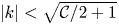 $|k|<\sqrt {\mathcal {C}/2+1}$ are growing) and that the fastest growing mode is only generated by nonlinear interactions. The result is a morphology diagram given in figure 6, which shows that the dominant mode of the limiting shape (e.g. number of fingers) is an increasing, piecewise constant function of
 $\mathcal {C}$ where there are sharp transitions from
 $k$-fold to
 $(k+1)$-fold dominant limiting shapes. While the morphologies of the limiting shapes are not identical, the dominant mode is solely determined by the constant
 $\mathcal {C}$. For reference, we also plot the maximum growing mode
 $k_{max}$ (solid curve). Although linear theory provides a good approximation of the dominant mode of the limiting shape, nonlinear interactions are critical for determining where the transitions from
 $k$-fold to
 $(k+1)$-fold dominant limiting shapes occur. Further, the range of
 $\mathcal {C}$ for which the limiting shape is dominated by a particular mode
 $k$ is an increasing function of
 $\mathcal {C}$.
A morphology diagram that relates the dominant mode of the limiting shapes (number of fingers) to the constant  $\mathcal {C}$ using the special gap dynamics
 $b_{\mathcal {C}}(t)=(1-({7}/{2})\tau \mathcal {C}t)^{-{2}/{7}}$, with
 $\tau =1\times 10^{-4}$ and
 $\mathcal {C}$ is varied from 52 to 1000. According to linear theory, the fastest growing mode
 $k_{max}$ (solid curve) varies from 3 to 12. The dots represent nonlinear numerical simulations using the same initial data (see text for details). The results suggest that the dominant mode of the limiting shapes are selected by
 $\mathcal {C}$. Linear theory provides a good approximation of the dominant modes, but nonlinear interactions dictate where transitions from
 $k$-fold to
 $(k+1)$-fold dominant limiting shapes occur.

In appendix C, we present cases where the initial condition contains modes that grow. In these cases, the dominant mode of the limiting shape can be dependent on the initial condition as well as  $\mathcal {C}$ (see figure 13). However, if the initial shape contains
 $k_{max}$ with magnitude comparable to the other initially growing modes, then the dominant mode of the limiting shape is still given by
 $k_{max}$, e.g. the limiting shape is still solely selected by
 $\mathcal {C}$ (see figure 14).
We have also investigated the angles between the thin fingers. In figure 7, we show the angles between pairs of fingers for drop morphologies from the morphology diagram (figure 6) as a function of symmetry mode  $k$. Several characteristic drop morphologies are shown as insets, where the smallest and largest angles between pairs of fingers are marked. For each symmetry mode
 $k$, the average of angles is close to
 $360/k$ (green curve) although fingers do not seem to intersect at one common point when
 $k$ is large. Note there are some cases in which some angles deviate significantly from the average (blue morphologies), which reflects the importance of nonlinearities. These happen when the interface conditions are close to transitions from
 $k$ to
 $k+1$ mode symmetries. The red morphologies show cases when all angles are close to its average.
The angles between pairs of fingers for drop morphologies from the morphology diagram (figure 6) are plotted as a function of the symmetry mode  $k$. The green curve indicates the angle
 ${360}/{k}$. Several characteristic drop morphologies at
 $k=3$,
 $5$,
 $8$ and
 $10$ are shown as insets, where the smallest and largest angles between fingers are marked in the corresponding inset. The blue morphologies show cases when some angles deviate most from
 $360/k$ and the red morphologies show cases when all angles are close to
 $360/k$.

4. Conclusions
In this paper, we have investigated the fully nonlinear dynamics of viscous drops in Hele-Shaw cells when the upper plate is lifted perpendicularly at a prescribed rate. This action reduces the size of drops in the midplane between the plates and increases the extent of the drops in the  $z$-direction to preserve volume. As air rushes in, this generates a Saffman–Taylor instability and the drops deform as they shrink. Linear theory predicts that the instability may be transient, if the lifting rate is sufficiently small, or may persist if the rate is sufficiently large. To simulate the nonlinear dynamics of the drops, we used a very efficient, highly accurate boundary integral method that involves space and time rescaling to track the shrinking of the drops in the midplane using the Hele-Shaw approximation (Zhao et al. Reference Zhao, Li, Yin, Belmonte, Lowengrub and Li2018). By rescaling time to slow down the rapid evolution of the drops and rescaling space to maintain constant-volume drops in the simulation frame, we can overcome the severe constraints on the time steps and spatial grid sizes that would be encountered in the original frame of reference. This enabled us to study the limiting dynamics as the drops vanish over a wide range of lifting rates.
We compared the nonlinear simulation results with linear theory and with previously performed experiments with two different surface tensions when the gap is increased linearly in time. Comparisons with a new experiment using a gap width that increases nonlinearly in time are presented in appendix E (figures 16–18). In these cases, the instability is transient and the drops eventually shrink like circles.
When the gap grows linearly in time, we found that nonlinear interactions increase perturbations more rapidly than predicted by linear theory. The nonlinear simulations tend to agree best with experiments at large confinement numbers ( $C_0={R_0}/{b_0}$, where
 $R_0$ is the initial radius of the liquid and
 $b_0$ is the initial gap) and predict a biphasic exponential decay of the number of fingers over time consistent with experiments. At small
 $C_0$, the nonlinear simulations overpredict the number of fingers. We suggested that this might be due to an increase in the wetting layer thickness, which scales as
 $h\sim C_0^{-4/3}$ as the confinement number decreases. By increasing the speed of the lifting plate, to mimic the more rapid loss of fluid to the wetting layer, we found better agreement between the simulations and experiments. Of course, in addition to wetting, other effects such as viscous stresses, inertial forces and three-dimensionality could also play an important role in the drop dynamics.
We also studied the limiting dynamics of drops when the gap is lifted very fast:  $b_{\mathcal {C}}(t)=(1-({7}/{2})\tau \mathcal {C} t)^{-{2}/{7}}$, where
 $\tau$ is the non-dimensional surface tension and
 $\mathcal {C}$ is a constant. According to linear theory, this gap, which diverges at the finite time
 $T_C=2/(7\tau \mathcal {C})$, ensures that mode
 $k=\sqrt {(1+\mathcal {C}/2)/3}$ is the fastest growing mode along the interface at any time. By rescaling in both time and space, we are now able to study the nonlinear limiting shapes as the drops vanish in this regime.
Consistent with linear theory, nonlinear simulations predict that the instability is transient when the gap  $b(t)$ satisfies
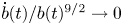 ${\dot {b}(t)}/{b(t)^{9/2}}\to 0$ as
 $t$ increases, even if the gap
 $b(t)$ diverges at a finite time. For example, in appendix D, we show that using the gap
 $b(t)=(1-3\tau \mathcal {C}t)^{-1/3}$, which diverges at
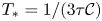 $T_*=1/(3\tau \mathcal {C})$ even faster than
 $b_{\mathcal {C}}(t)$, the interface undergoes a transient instability but ultimately vanishes like a circle since
 ${\dot {b}(t)}/{b(t)^{9/2}}\sim (T_*-t)^{1/6}$ as
 $t\to T_*$ (see figure 15). However, when the gap
 $b_{\mathcal {C}}(t)$ is used, perturbations may continually grow and the drop morphologies may acquire a striking, one-dimensional web-like shape as the drops shrink. To our knowledge, this limiting behaviour has not been reported previously.
We characterized the limiting drop shapes by generating a morphology diagram that relates the number of fingers to  $\mathcal {C}$, independent of initial conditions within a class of interface shapes that contains only high mode interface perturbations so that the most unstable mode is generated solely by nonlinear interactions. While linear theory provides a good approximation of the dominant modes, nonlinear interactions determine where transitions (in
 $\mathcal {C}$) from
 $k$-fold to
 $k+1$-fold dominant limiting shapes occur. We also described the behaviour of the system when low mode perturbations are present initially.
A natural question is whether the one-dimensional, web-like shapes we have discovered here when the upper plate is lifted very rapidly are actually achievable in an experiment. Depending on the initial conditions, our simulations suggest that the web-like shapes can be observed when the radius decreases from its initial value by approximately a factor of 7–10 (figure 14). This corresponds to an increase in gap width by a factor of approximately 50–100. If the initial gap  $b_0=50\ \mathrm {\mu }\textrm {m}$, this corresponds to a final gap thickness of approximately
 $b\sim 2.5\text{--}5\ \textrm {mm}$. Assuming that the gap width increases by a factor of 100, the corresponding time over which this would occur is
 $\mathcal {T}\sim ({0.29}/{\mathcal {C}\tau }) T$, where
 $T$ is a characteristic time scale given by
 $T\sim ({12\mu }/{\sigma })C_0^2R_0\tau$ where
 $\mu$ and
 $\sigma$ are the dimensional viscosity and surface tension, respectively, and
 $C_0=R_0/b_0$ is the confinement number with
 $R_0$ being the initial drop radius. This gives
 $\mathcal {T}\sim ({0.29}/{\mathcal {C}}) ({12\mu }/{\sigma })C_0^2R_0$. Using the values of the viscosity and surface tension from Nase et al. (Reference Nase, Derks and Lindner2011) to be
 $\mu =10\ \textrm {Pa}\ \textrm {s}$ and
 $\sigma =0.02\ \textrm {N}\ \textrm {m}^{-1}$, respectively, and the initial radius
 $R_0=1.5\ \textrm {mm}$, we obtain
 $\mathcal {T}\sim {2349}{\mathcal {C}^{-1}}\ \textrm {s}$ since
 $C_0=R_0/b_0=30$. Finally, taking
 $\mathcal {C}=2(3k^2-1)$ we obtain
 $\mathcal {T}=\mathcal {T}_k\sim {1200}/({3k^2-1})\ \textrm {s}$. So as the dominant mode
 $k$ of the limiting shape increases, the time over which the plate needs to be lifted decreases as
 $k^{-2}$. For example, for 3-mode dominant limiting shapes we obtain
 $\mathcal {T}_3\sim 46\ \textrm {s}$ while for 4-mode and 5-mode dominant shapes we obtain
 $\mathcal {T}_4\sim 25\ \textrm {s}$ and
 $\mathcal {T}_5\sim 16\ \textrm {s}$, respectively. The two-dimensional approximation fails when
 ${\tilde {b}(\tilde {t})}/{\tilde {R}(\tilde {t})}\sim O(1)$ and we estimate the corresponding time
 $\mathcal {T}^D\sim (1-C_0^{-7/3})\mathcal {T}$. For
 $C_0=30$,
 $\mathcal {T}^D$ is
 $0.01\ \textrm {s}$ earlier than
 $\mathcal {T}$. This suggests that it should be possible to access this regime experimentally, at least for limiting shapes dominated by low modes.
Once experiments in the special gap regime are performed, agreement between theory and experimental results may also require accounting for the effects of flow in three dimensions (Ben Amar & Bonn Reference Ben Amar and Bonn2005), wetting effects (Park & Homsy Reference Park and Homsy1984; Park et al. Reference Park, Gorell and Homsy1984; Dias & Miranda Reference Dias and Miranda2013a) and inertia effects (Chevalier et al. Reference Chevalier, Ben Amar, Bonn and Lindner2006; He & Belmonte Reference He and Belmonte2011; Anjos et al. Reference Anjos, Dias and Miranda2017), which were neglected in our Hele-Shaw formulation. These will be considered in future work.
Acknowledgements
S.L. and J.L. gratefully acknowledge partial support from the National Science Foundation, Division of Mathematical Sciences through grants NSF-DMS 1719960 (J.L.) and NSF-DMS 1720420 (S.L.). J.L. also acknowledges partial support from grants NSF-DMS 1763272 and the Simons Foundation (594598, QN) for the Center for Multiscale Cell Fate Research at UC Irvine. The authors are also grateful for insightful and helpful comments from anonymous reviewers.
Declaration of interests
The authors report no conflict of interest.
Appendix A. Modified lifting speed of experiments in Nase et al. (Reference Nase, Derks and Lindner2011)
In the manuscript, we compared our simulation results, linear theory and experimental results from Nase et al. (Reference Nase, Derks and Lindner2011). In the experiments, the bottom plate of a Hele-Shaw cell is fixed and the top plate is lifted uniformly at a constant speed. A less viscous fluid (air) penetrates a more viscous fluid (silicone oil), forming fingering patterns on the interface. High resolution, high contrast images are used to calculate the number of fingers (Nase et al. Reference Nase, Derks and Lindner2011). The fingertip is described as the innermost part of an air finger and the finger base is the outer end of a finger (see figure 8). The finger amplitude is the distance between the tip and base of a finger. In Nase et al. (Reference Nase, Derks and Lindner2011), the authors systematically investigate the influence of different parameters on the dynamics of the drop evolution, including how the number of fingers varies as a function of time. To do this, the initial drop size, the initial gap spacing and the lifting speed are varied. The number of fingers not only depends on the non-dimensional surface tension  $\tau$ but also on the confinement number
 $C_0={R_0}/{b_0}$, the aspect ratio of the fluid. When the surface tension is large, the effect of
 $C_0$ is more pronounced at later times while at small surface tensions,
 $C_0$ has a larger effect at early times, see Nase et al. (Reference Nase, Derks and Lindner2011) for further details.
A schematic of an interface and definition of the finger tip, finger base and finger amplitude, following Nase et al. (Reference Nase, Derks and Lindner2011). See text for details.

To extract the number of fingers over time from the experiments, we use the data presented in figure 10(c,e) in Nase et al. (Reference Nase, Derks and Lindner2011) and use the web application WebPlotDigitizer (https://automeris.io/WebPlotDigitizer/) to extract the data points. In particular, after choosing the scale of the plot, we are able to get the position of each data point on the plots where the number of fingers is usually a decimal close to an integer. Since the number of fingers is an integer, we round to the nearest integer. As pointed out in Nase et al. (Reference Nase, Derks and Lindner2011) the number of fingers depends on both the surface tension and the confinement number. At small confinement numbers  $C_0$ (see figure 9a,b), the number of fingers shows a single rate of exponential decay over time, consistent with the experimental results in Ben Amar & Bonn (Reference Ben Amar and Bonn2005). At large confinement numbers
 $C_0$ (see figure 9c,d), the number of fingers seems to have a biphasic exponential decay in time, similar to our simulation results.
The number of fingers in drops with different confinement number  $C_0$ from the experiments in Nase et al. (Reference Nase, Derks and Lindner2011) with surface tension
 $\tau =3\times 10^{-5}$. At small
 $C_0$ the number of fingers follows a single rate of exponential decay in time while the data at large
 $C_0$ suggests that there is a biphasic exponential decay in the number of fingers over time. (a)
 $C_0 = 30$, (b)
 $C_0 = 40$, (c)
 $C_0 = 54.5$, (d)
 $C_0 = 120$.

In our simulations, we calculate the number of air fingers in exactly the same way as Nase et al. (Reference Nase, Derks and Lindner2011). We have found that our simulation results agree very well with the experimental observations at large confinement numbers  $C_0$ and predict more fingers than the experimental data at small confinement numbers
 $C_0$. It is still not well understood how the confinement number influences the behaviour of the drop. One possibility might be the volume loss of the drop fluid as the fluid is stuck to the plate. Consequently, the effective shrinking speed of the fluid in experiments might be faster than the constant speed we assumed in our simulations.
To test this hypothesis, we analyse the dependence of the wetting layer thickness on the confinement number. The thickness of the wetting layer on the plate  $h$ is proportional to
 $\textit {Ca}^{2/3}$, where
 $\textit {Ca}=\mu \tilde {V}/\sigma$ is the capillary number (Park & Homsy Reference Park and Homsy1984; Park et al. Reference Park, Gorell and Homsy1984; Jackson et al. Reference Jackson, Stevens, Giddings and Power2015). Using
 $\tilde {V}\sim \dot {\tilde {b}}_0C_0$, we obtain
 $\textit {Ca}\sim (\mu \dot {\tilde {b}}_0/\sigma )C_0$. In the experiments (Nase et al. Reference Nase, Derks and Lindner2011), the confinement number and lifting rate are changed such that the non-dimensional surface tension
 $\tau =\sigma \tilde {b}_0^3/(12\mu \dot {\tilde {b}}_0 R_0^3)$ is fixed. This gives
 $\textit {Ca}\sim C_0^{-2}$ and therefore
 $h\sim C_0^{-4/3}$. This implies that the wetting layer gets thicker as the confinement number
 $C_0$ decreases. That is, more fluid is stuck on the plate and the fluid has a faster effective shrinking speed as the confinement number
 $C_0$ decreases.
To investigate the increase in wetting layer thickness due to  $C_0$, we make a correction to our lifting speed in the simulations and consider
 $b(t)=1+(({1+3e_0t})/({1+3t}))t$, where
 $e_0$ is a constant accounting the speed change. This correction is ad-hoc and a simple way to account for the additional volume loss of drop fluid to the wetting layer. Future work should account for the boundary layer dynamics directly. Note that
 $e_0=1$ corresponds to the original formulation (linear rate of gap increase). However, the larger
 $e_0$ is, the more fluid is left on the plates and the faster effective shrinking speed is. We take different
 $e_0=1$,
 $1.1$,
 $1.3$,
 $1.5$ and
 $1.7$ and perform simulations using this lifting speed. The results are shown in figure 10(a,b). The morphologies of the interface using
 $e_0=1.2$ (figure 10a) and
 $e_0=1.7$ (figure 10b) are shown as insets. At early times, the number of fingers is insensitive to the choice of
 $e_0$. At later times, the number of fingers decreases as
 $e_0$ increases. By treating
 $e_0$ as a fitting parameter, our simulations can fit the experimental data for all confinement numbers
 $C_0$ using the modified gap dynamics.
Comparisons between the experimental data from Nase et al. (Reference Nase, Derks and Lindner2011) (with surface tension  $\tau =3\times 10^{-5}$; shown also in figure 9) and simulations using the modified gap
 $b(t)=1+(({1+3e_0t})/({1+3t}))t$ to account for the volume loss of the fluid drop due to changes in the wetting layer thickness due to confinement (see text for details). Increasing the thickness corresponds to increases in
 $e_0$ as more fluid is stuck to plates. (a) Results at large confinement numbers
 $C_0$ with
 $e_0$ as labelled. The interface morphologies, with
 $e_0=1.2$, are shown at different times in the insets. (b) Results at small
 $C_0$ with
 $e_0$ as labelled. The interface morphologies, with
 $e_0=1.7$, are shown at different times in the insets. As
 $e_0$ increases, the number of fingers decreases. Treating
 $e_0$ as a fitting parameter, the simulations can fit the experimental data over the whole range of confinement numbers considered.

Appendix B. Examples of dynamics dominated by mode 3
In figure 11, we exhibit the interfacial dynamics in the rescaled frame under a special gap  $b_{\mathcal {C}}=(1-({7}/{2})\tau \mathcal {C}t)^{-2/7}$ with
 $\mathcal {C}=52$ and non-dimensional surface tension
 $\tau =1\times 10^{-4}$. With these parameters, the linear fastest growing mode is 3. We take three different initial shapes:
 $r(\alpha ,0)=1+0.02(\cos (3\alpha )+\cos (5\alpha )+\cos (6\alpha ))$ (blue);
 $r(\alpha ,0)=1+0.02(\cos (3\alpha )+\sin (7\alpha )+\cos (15\alpha )+\sin (25\alpha ))$ (magenta);
 $r(\alpha ,0)=1+ 0.02(\sin (6\alpha )+\cos (15\alpha )+\sin (25\alpha ))$ (red). All three cases show that after a period of transient morphological changes, the drop morphologies eventually acquire a 3-fold symmetric, one-dimensional, web-like network structure as they vanish. Since mode 3 is not initially present in the third case (red), it takes some time for nonlinear interactions to generate mode 3 and for mode 3 to dominate the shape. As a result, a longer time has to pass for the corresponding (red) drop morphologies to acquire 3-fold dominant shapes and as a result the drop is much smaller than the others when this occurs.
The drop dynamics in the rescaled frame under the special gap  $b_{\mathcal {C}}=(1-({7}/{2})\tau \mathcal {C}t)^{-2/7}$ with
 ${\mathcal {C}=52}$, where mode 3 grows fastest according to linear theory. Here we take the non-dimensional surface tension
 $\tau =1\times 10^{-4}$. (a–d) The evolution under the initial condition
 $r(\alpha ,0)=1+0.02(\cos (3\alpha )+\cos (5\alpha )+\cos (6\alpha ))$. (e–h) The evolution under the initial condition
 $r(\alpha ,0)=1+0.02(\cos (3\alpha )+\sin (7\alpha )+\cos (15\alpha )+\sin (25\alpha ))$. (i–l) The evolution under the initial condition
 $r(\alpha ,0)=1+0.02(\sin (6\alpha )+\cos (15\alpha )+\sin (25\alpha ))$. In all cases, the limiting shape tends to a 3-fold symmetric, one-dimensional web-like structure.

In the main manuscript, we have shown the length of the neck region tends to be finite. Consequently, the lengths of the long filaments in the rescaled frame increase as the drop sizes decrease. In figure 12(a), we show the drop dynamics in the rescaled frame from the initial shape  $r(\alpha ,0)=1+0.02(\cos (3\alpha )+\cos (5\alpha )+\cos (6\alpha ))$ and the special gap
 $b_{\mathcal {C}}=(1-(7/2)\tau \mathcal {C}t)^{-2/7}$ with
 $\mathcal {C}=52$, where mode 3 grows fastest linearly. As the drop shrinks, the interface tends to form a bud at the far end and a smooth fingertip at the inner end, connected by a long filament. The inset, which focuses on the boxed region, shows that the filaments get thinner and longer as the size of the drop decreases. We also find the perimeter of the interface
 $P$ decreases linearly in
 $R$ to a finite length as
 $R$ decreases. As the gap width is changed to select other symmetry modes of the limiting shapes, the corresponding interface perimeters still decrease linearly in
 $R$ but with different slopes (figure 12b). The slopes decrease as the symmetry of the interface increases. In this case, the initial condition for each interface is
 $r(\alpha ,0)=1+0.02\cos (k\alpha )$ where
 $k=$ 3, 4, 5, 6 and 7. The corresponding (special) gap dynamics are
 $b_{\mathcal {C}}=(1-({7}/{2})\tau \mathcal {C}t)^{-2/7}$ with
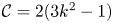 $\mathcal {C}=2(3k^2-1)$. As expected, the morphology of each drop is dominated by mode
 $k$. Comparing the slope of the 3 mode symmetry here and the slopes in figure 3(c) in the main manuscript, we find that the slopes are close and differences are likely due to the initial condition, which is different.
Details of the drop morphologies. We reverse the orientation of the horizontal axis to reflect the fact that the radius  $R$ decreases with time
 $t$. (a) The drop dynamics in the rescaled frame near the vanishing time corresponding to figure 3(b) in the main text, which shows the drop morphologies in the original frame. The inset shows a blow-up of the neck region in the boxed region. (b) The relation between the perimeter of the interface
 $P$ and the effective radius
 $R$ for different symmetric limiting shapes (see text for details) using the special gap
 $b_{\mathcal {C}}=(1-({7}/{2})\tau \mathcal {C}t)^{-2/7}$, where
 $\tau =1\times 10^{-4}$,
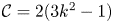 $\mathcal {C}=2(3k^2-1)$ and
 $k$ varies as 3, 4, 5, 6 and 7. (c) The maximum curvature of the far end in the rescaled frame with respect to
 $R$. (d) The minimum curvature of the inner end in the rescaled frame with respect to
 $R$.

In figure 12(c,d) we show the maximum (minimum) curvature at the far end (the inner end) in the rescaled frame for the drop interfaces shown in figure 11. We fit the curvatures as a power function of  $R$ (solid line), which indicates the curvatures tend to a finite number as
 $R\rightarrow 0$. While the minimum curvature at the inner end may not be the same for different initial conditions, the maximum curvature at the far end tends to approach the same limit
 $\bar {\kappa }_*\approx 5.8$. This suggests that the buds at the far end may acquire a universal shape that is independent of the initial conditions. From figures 3(b) and 4(a) in the main manuscript, we see that the length of the filaments approaches a finite number. Approximating the filaments as a rectangle with a circular tip with radius
 $\bar {\kappa }_*/R$, the perimeter
 $P\sim P_0+aR$, where
 $a$ is a constant related to
 $\bar {\kappa }_*$ and
 $P_0$ is a finite number depending on the initial shape. This explains why the perimeter decreases as a linear function of
 $R$, as seen in figure 12(b).
Appendix C. Active lower modes under the special gap dynamics  $b_{\mathcal {C}}(t)= (1-({7}/{2})\tau \mathcal {C}t)^{-{2}/{7}}$

As we have shown in the manuscript, the dominant mode of the morphology is solely determined by the control parameter  $C$ if the initial shape only contains high modes,
 \begin{equation} r(\alpha,0)=1+\epsilon\sum_{k=k_{min}}^{k_N}\textrm{e}^{-\beta k}(a_k\cos(k\alpha)+b_k\sin(k\alpha)), \end{equation}
where  $\epsilon =2.5\times 10^{-3}$,
 $\beta =0.2$,
 $k_{min}=30$,
 $k_{max}=60$, and
 $a_k$ and
 $b_k$ are uniformly distributed in
 $(-1, 1)$. All these high modes are stable and tend to vanish. However, lower modes are created by nonlinear interactions and depending on
 $\mathcal {C}$, a particular mode
 $k_{max}$ will have the fastest growth rate and will finally dominate the morphology of drop. This is still true if lower modes are present in the initial condition. These modes may be active in the sense that they may grow due to the Saffman–Taylor instability. In figure 13, we report the results with lower modes present in the initial condition. Using the gap as
 $b_{\mathcal {C}}(t)=(1-({7}/{2})\tau \mathcal {C}t)^{-{2}/{7}}$, where
 $\mathcal {C}=484$, linear theory suggests mode 9 grows fastest and our simulations show a 9-fold shape if the initial shape only contains modes 30 to 60 (first row). If the initial conditions contain low modes, the results can be different. For example, simulations show that a 13-fold shape emerges when modes from 13 to 60 are present initially (figure 13e–h) and a 5-fold shape emerges when the initial data contains modes from 5 to 60 (figure 13i–l). The reason is these low modes are active all the time and their initial perturbations are much larger than the perturbation of mode 9 because of the form of the initial condition in (C 1). For instance, in the second row the initial magnitude of mode 13 is approximately
 $1.857\times 10^{-4}$ while mode 9 does not appear in the initial shape. For the third row the initial magnitude of mode 5 is approximately
 $9.19\times 10^{-4}$, which is approximately twice the magnitude of mode 9 initially. Even though mode 9 grows faster than all the other modes, there is not enough time for mode 9 to dominate the shape. To demonstrate this, we add mode 9 to these initial shapes such that mode 9 has the same magnitude as that of the smallest mode. Figure 14 shows that in this case, mode 9 is selected and morphologies tend to a 9-fold dominant shape.
The drop morphologies using the special gap  $b_{\mathcal {C}}(t)=(1-({7}/{2})\tau \mathcal {C}t)^{-{2}/{7}}$ with
 $\mathcal {C}=484$, which makes mode 9 the fastest growing mode from linear theory. When the initial shape does not contain lower unstable (active) modes (e.g. modes 30–60), the interface develops a 9-fold dominant shape (a–d). When there exist lower active modes, the interfaces develop a 13-fold shape (when modes 13–60 are present in the initial condition) and a 5-fold shape (when modes 5–60 are contained in the initial condition). See text for details.

The drop morphologies using the special gap  $b_{\mathcal {C}}(t)=(1-({7}/{2})\tau \mathcal {C}t)^{-{2}/{7}}$ with
 $\mathcal {C}=484$ (mode 9 is the fastest linearly growing mode) but with initial conditions that are the same as in figures 13(e–h) and 13(i–l) except that in each case, mode 9 has been added into the initial condition with the same magnitude as modes 13 (a–d) and 5 (e–h), respectively. In both cases the morphologies are dominated by mode 9 as the drop shrinks.

Appendix D. Other choices of gap dynamics
According to linear theory (given in the main text), the critical gap width is determined by the relation that  $\dot {b}(t)/b(t)^{9/2}$ is a constant in time (see (2.10)). Therefore, if
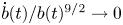 ${\dot {b}(t)/b(t)^{9/2} \to 0}$ as time increases, the drop should eventually shrink like a circle, even if the gap width blows up at a finite time. For example,
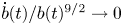 $\dot {b}(t)/b(t)^{9/2} \to 0$ when
 $b(t)=1+t$,
 $b(t)=\textrm {e}^t$ or even
 $b_{\mathcal {D}}(t)=(1-3\tau \mathcal {D}t)^{-1/3}$, for any
 $\mathcal {D}$. In the latter case, the rate of blow up is actually larger than that for the special gap
 $b_{\mathcal {C}}(t)$. To confirm this behaviour, we perform nonlinear simulations using
 $b_{\mathcal {D}}(t)$ for different choices of
 $\mathcal {D}$. The results are shown in figure 15. We observe that for each case considered, the drop eventually shrinks like a circle after a transient instability, which confirms the predictions of linear theory. The initial condition for each simulation is
 $r(\alpha ,0)=1+0.02(\cos (3\alpha )+\cos (5\alpha )+\cos (6\alpha ))$ and the drop morphologies using
 $\mathcal {D}=100$ are shown as insets.
The relative perturbation magnitude of drop interfaces, as a function of  $R$, using the gap
 $b_{\mathcal {D}}(t)=(1-3\tau \mathcal {D}t)^{-1/3}$ with
 $\mathcal {D}$ as labelled. Insets show the drop interfaces with
 $\mathcal {D}=100$ and
 $\tau =1\times 10^{-4}$. In all cases, the drop shrinks like a circle after a transient instability. We reverse the orientation of the horizontal axis to reflect the fact that the radius
 $R$ decreases with time
 $t$.

Appendix E. Comparison with experimental data under a nonlinear gap width
We next compare the simulation results with an experiment in which the gap is increased nonlinearly in time. In the experiment, a thin layer of Canola oil is confined between two parallel plates. We use clear acrylic plates  $12\ \rm {in.} \times 12\ \rm {in.} \times 1/2\ \rm {in.}$ with an initial gap
 $b_0=100\ \mathrm {\mu }\textrm {m}$. The upper plate is lifted at two diagonal corners manually. The Canola oil purchased from Great Value has viscosity
 $\mu =65\ \textrm {cP}$ and surface tension
 $\sigma =31.3\ \textrm {mN}\ \textrm {m}^{-1}$. We use video images to capture the air–oil interface. The contour of the air–oil contact line is found by using IMAGEJ and MATLAB (see figure 16). However, since the plate is lifted by hand, the gap width may not be uniform in space. Nevertheless, we will assume the gap is spatially uniform in our simulations.
Image processing in the manual lifting plate experiment. (a) Top view of the drop in the Hele-Shaw cell (the scale bar is 5 m). (b) The fluid domain after applying thresholding in IMAGEJ. (c) The contour of the air–oil contact line extracted in MATLAB.

Because the upper plate is lifted manually, the time-dependent gap is unknown and nonlinear, but we are able to reconstruct the gap width from the area enclosed by the contact line  $A(\tilde {t})$, where
 $\tilde {t}$ is the dimensional time. We find the area of the oil
 $A(\tilde {t})$, fits the data using a smooth spline in MATLAB, and compute
 $A'(\tilde {t})$ using the spline (see figure 17a). Since there is fluid leftover on the plate due to a thick wetting layer, we assume that the rate of volume loss of the drop fluid is proportional to the area change
 \begin{equation} \frac{1}{V_{ol}}\frac{\textrm{d}V_{ol}}{\textrm{d}\tilde{t}}=e_1A'(\tilde{t}), \end{equation}
where  $V_{ol}$ is the volume of the drop and
 $e_1$ is a positive constant. The gap is then given as
 \begin{equation} b(\tilde{t})=\frac{b_0A(0)}{A(\tilde{t})}\exp(e_1(A(\tilde{t})-A(0))). \end{equation}
We have constructed the gap width with different parameters  $e_1$ in figure 17(b), where increasing
 $e_1$ decreases the gap width.
The drop areas and gap widths for experiments with nonlinear dynamics of the gap width. (a) The drop areas (*), the fitted area (solid line) and the computed  $A'$ (dashed line) in dimensional time
 $\tilde {t}$. (b) The gap widths reconstructed from the area
 $A(\tilde {t})$ as
 $b(\tilde {t})=({b_0A(0)}/{A(\tilde {t})})\exp (e_1(A(\tilde {t})-A(0)))$ under different
 $e_1$ as labelled. See text for details.

Taking the time scale to be  $T=-({A(0)}/{A'(0)})=0.3243$, the non-dimensional time is
 $t={\tilde {t}}/{T}$. At early times, the oil–air interface is nearly a circle, as figure 16(c). We find the initial equivalent radius of the interface is
 $R_0=2.349\ \textrm {cm}$ and the non-dimensional surface tension is
 $\tau =({\sigma b_0^2}/{12\mu R_0^3})T=1.0273\times 10^{-5}$. The experimental results are shown in figure 18(a–c) and simulations using different values of
 $e_1$ are shown in figure 18(d–l). In both the experiments and simulations, there is a transient instability as fingers are generated and grow towards the centre of the drop at early times before eventually decaying away at later times. Generally, there is good agreement between the simulations and experiments.
Morphologies of the drops with nonlinear gap dynamics from experiments (a–c) and simulations with different compensation parameters  $e_1=0$ (black; d–f),
 $e_1=0.012$ (magenta; g–i), and
 $e_1=0.019$ (blue; j–l) at the dimensional times
 $\tilde {t}=0.233$ (a,d,g,j),
 $0.3$ (b,e,h,k) and
 $0.366$ (c,f,i,l).



