1 Introduction
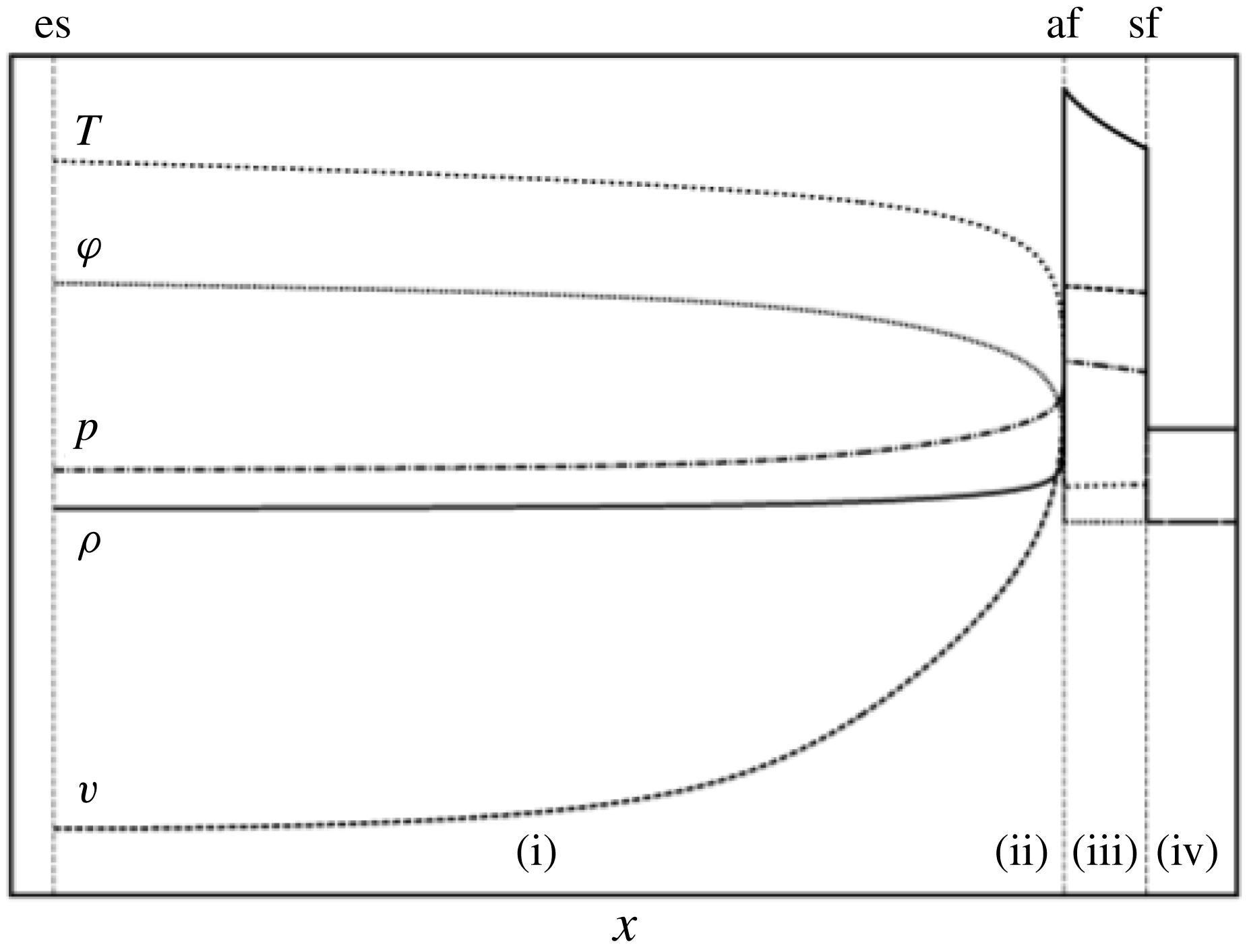
Deflagration waves driven by thermal radiation – or ‘radiative ablation waves’ – are encountered in certain stellar flows and, on Earth, in laboratory experiments of high energy density physics (HEDP), including those dedicated to inertial confinement fusion (ICF). Such waves may occur, for instance, when exposing an initially quiescent cold and opaque material to a growing thermal radiation (cf. Zel’dovich & Raizer Reference Zel’dovich and Raizer1967, chapter 10, § 8). The associated flow sees energy penetrating the cold material in the form of a leading shock wave followed, and sustained, by a steep heat front propagating at subsonic velocities – ‘ablation front’ – which coincides with the leading edge of a rarefaction wave (figure 1). This physical process is a rather efficient way of driving a fluid into motion at high velocities and is a key mechanism for creating laboratory radiation-driven implosions with the goal of achieving the conditions of thermonuclear burn in ICF (Atzeni & Meyer-ter-Vehn Reference Atzeni and Meyer-ter-Vehn2004).
Structure of an ablation wave driven by a nonlinear heat conduction. Spatial profiles in the Cartesian coordinate
 $x$
of the flow density
 $\unicode[STIX]{x1D70C}$
(
 $-\!\!-$
), velocity
 $v$
(
 $-\,-\,-$
), temperature
 $T$
(
 $\boldsymbol{\cdot }\boldsymbol{\cdot }\boldsymbol{\cdot }$
), heat flux
 $\unicode[STIX]{x1D711}$
(
 $\boldsymbol{\cdot }\!\boldsymbol{\cdot }\!\boldsymbol{\cdot }$
) and pressure
 $p$
(
 $-\,\boldsymbol{\cdot }\,-$
). Four regions typical of such flows are identified: (i) the conduction region extending from the irradiated external surface (es) and characterized by the inward propagation of heat (
 $\unicode[STIX]{x1D711}>0$
) altogether with the expansion of the fluid (
 $\unicode[STIX]{x2202}v/\unicode[STIX]{x2202}x>0$
); (ii) the deflagration, or ablation, layer associated with the subsonic thermal-wave front, or ‘ablation front’ (af), and identified by the steepest temperature and density gradients; (iii) the shock compressed fluid region, between the ablation layer and the leading shock-wave front (sf), with the highest densities; (iv) the undisturbed fluid region (
 $v=0$
) upstream to the shock front.

Several simplifying assumptions are commonly used for gaining insight into the physics of such flows: (i) the radiation heat-conduction approximation of radiative transfer, valid for optically thick materials remaining at local thermodynamic equilibrium (Zel’dovich & Raizer Reference Zel’dovich and Raizer1967); (ii) the dominance, at sufficiently high temperatures (thousands of degrees Kelvin), of diffusive effects due to radiation over those of thermal conduction and viscosity, except in shock fronts; (iii) negligible radiative pressure and energy compared with the material pressure and internal energy for not too high temperatures (below a few millions of degrees Kelvin). These assumptions comply rather well with conditions of fusion-target implosions driven by cavity – or ‘hohlraum’ – generated X-rays in current ICF laser facilities (e.g. Lindl et al. Reference Lindl, Landen, Edwards and Moses2014). Accordingly, the equations of radiation hydrodynamics are reduced to the Euler equations with nonlinear heat conduction, owing to the fluid opacity dependence on temperature. At the very inception of investigations on radiation-driven flows, Marshak (Reference Marshak1958) exhibited and exploited a similarity transformation of these equations in plane symmetry. This transformation was established for a semi-infinite slab of a polytropic gas – with an opacity (equivalently, heat-conduction coefficient) in powers of the density and temperature – taken initially quiescent, perfectly cold and homogeneous, and subject to a boundary surface temperature following a time power law imposed by the opacity temperature exponent (Marshak Reference Marshak1958, § II.C). Based on numerical solutions of the transformed equations for increasing values of the surface temperature parameter, the full range of behaviours between radiative shock waves, subsonic (i.e. deflagration) and supersonic radiation heat waves was reported. Besides, the two limiting cases of a constant-density supersonic and of a constant-pressure subsonic radiation wave were considered, leading to approximate self-similar analytical descriptions of the wave fronts, or ‘Marshak waves’ (Marshak Reference Marshak1958, § II.B).
Following this seminal work, self-similar solutions of the radiation hydrodynamics equations were proposed and computed for other assumptions of interest: e.g. additional types of symmetry (i.e. spherical, cylindrical), less restrictive modelling of radiative transfer or thermal conduction, inhomogeneous initial state of the fluid (Elliott Reference Elliott1960; Wang Reference Wang1964; NiCastro Reference NiCastro1970; Ghoniem et al. Reference Ghoniem, Kamel, Berger and Oppenheim1982). Some of these works, performed in the context of a strong point explosion, recovered or extended results summarized in (Sedov Reference Sedov1959, chapter 4, § 11) on the self-similar spherical blast-wave problem of gas dynamics with nonlinear heat conduction. Numerical integration of the system of ordinary differential equations (ODEs) resulting from the exact similarity transformation of Marshak (Reference Marshak1958, § II.C) was reconsidered in some detail by Bajac (Reference Bajac1973), then treated more thoroughly in unpublished work of 1983 by Saillard (cf. Abéguilé et al. Reference Abéguilé, Boudesocque-Dubois, Clarisse, Gauthier and Saillard2006). In connection with hohlraum-radiation-driven flows, Pakula & Sigel (Reference Pakula and Sigel1985) investigated the self-similar planar ablation of an infinitely dense material as the large time limit of the ablation of semi-infinite slabs. In a broader prospect, Coggeshall & Axford (Reference Coggeshall and Axford1986) studied the invariance under Lie group transformations of the radiative hydrodynamics equations in the radiation conduction approximation for planar, cylindrical or spherical symmetries, and thus extended the set of known similarity solutions to these equations. The self-similar blast-wave problem with nonlinear heat conduction was reconsidered in Reinicke & Meyer-ter-Vehn (Reference Reinicke and Meyer-ter-Vehn1991) with a complete similarity analysis in terms of Lie group symmetry, a detailed study of the solution singularities and numerical examples. Still on the basis of Marshak’s exact similarity transformation, solutions in the particular case of tamped radiative ablation were analysed in Sanz, Piriz & Tomasel (Reference Sanz, Piriz and Tomasel1992) by means of piecewise approximate solutions. A further step in the description of these exact similarity solutions was achieved when numerical computations of ablative flows, with a level of accuracy compatible with a hydrodynamic stability analysis, were obtained by some of the present authors (Boudesocque-Dubois, Clarisse & Gauthier Reference Boudesocque-Dubois, Clarisse, Gauthier, Kálal, Rohlena and Šiňor2001; Abéguilé et al. Reference Abéguilé, Boudesocque-Dubois, Clarisse, Gauthier and Saillard2006; Boudesocque-Dubois, Gauthier & Clarisse Reference Boudesocque-Dubois, Gauthier and Clarisse2008). A different similarity transformation, which corresponds to the non-stationary acceleration of an ablatively driven planar foil, until its burning out, was pointed out in Murakami, Sakaiya & Sanz (Reference Murakami, Sakaiya and Sanz2007). In a more model-oriented approach and in relation with hohlraum-wall hydrodynamics in HEDP experiments, approximate and exact self-similar descriptions of supersonic and subsonic radiative waves, based on the solutions of Marshak (Reference Marshak1958) and Pakula & Sigel (Reference Pakula and Sigel1985), have been proposed for fluid internal energy in powers of the fluid density and temperature (Hammer & Rosen Reference Hammer and Rosen2003; Garnier et al. Reference Garnier, Malinié, Saillard and Cherfils-Cléouin2006; Shussman & Heizler Reference Shussman and Heizler2015), in place of the original polytropic-gas energy law.
Supersonic or subsonic heat-wave flows driven by nonlinear, including radiative, heat conduction present steep heat fronts due to the temperature nonlinearity of the diffusion process. This steepness – at the origin of the approximate self-similar treatments of Marshak (Reference Marshak1958) and others – motivated the investigation by Fraser (Reference Fraser1960) of steadily propagating radiation fronts and their descriptive classification into subsonic (‘radiation flames’) and supersonic (‘radiation shocks’) families. Independently, Samarskiĭ, Kurdyumov & Volosevich (Reference Samarskiĭ, Kurdyumov and Volosevich1965) studied travelling-wave solutions of gas dynamics with nonlinear heat conduction and identified the wave structures that subsonic and supersonic waves may present. The description of steady radiative ablation was pursued and carried out, with the purpose of modelling ICF related flows, by Nozaki & Nishihara (Reference Nozaki and Nishihara1980), Nishihara (Reference Nishihara1982), Saillard, Arnault & Silvert (Reference Saillard, Arnault and Silvert2010); cf. also (Atzeni & Meyer-ter-Vehn Reference Atzeni and Meyer-ter-Vehn2004, § 7.7). The corresponding models connect a steadily moving ablation layer to an isothermal – necessarily unsteady – expansion into vacuum, at a Chapman–Jouguet point defined relatively to the heat front. Within the approximation of radiation heat conduction, this isothermal assumption can only be verified in the limiting case of an infinite conduction coefficient. For finite conductivity, a temperature stratification persists throughout the heated fluid region up to the fluid external boundary with the consequence that a definition of the ablation layer thickness can only be arbitrary (Fraser Reference Fraser1960). This extensive stratification is a characteristic feature of ablation waves driven by radiation, or strongly nonlinear heat conduction that distinguishes them from deflagration waves encountered in slow combustion.
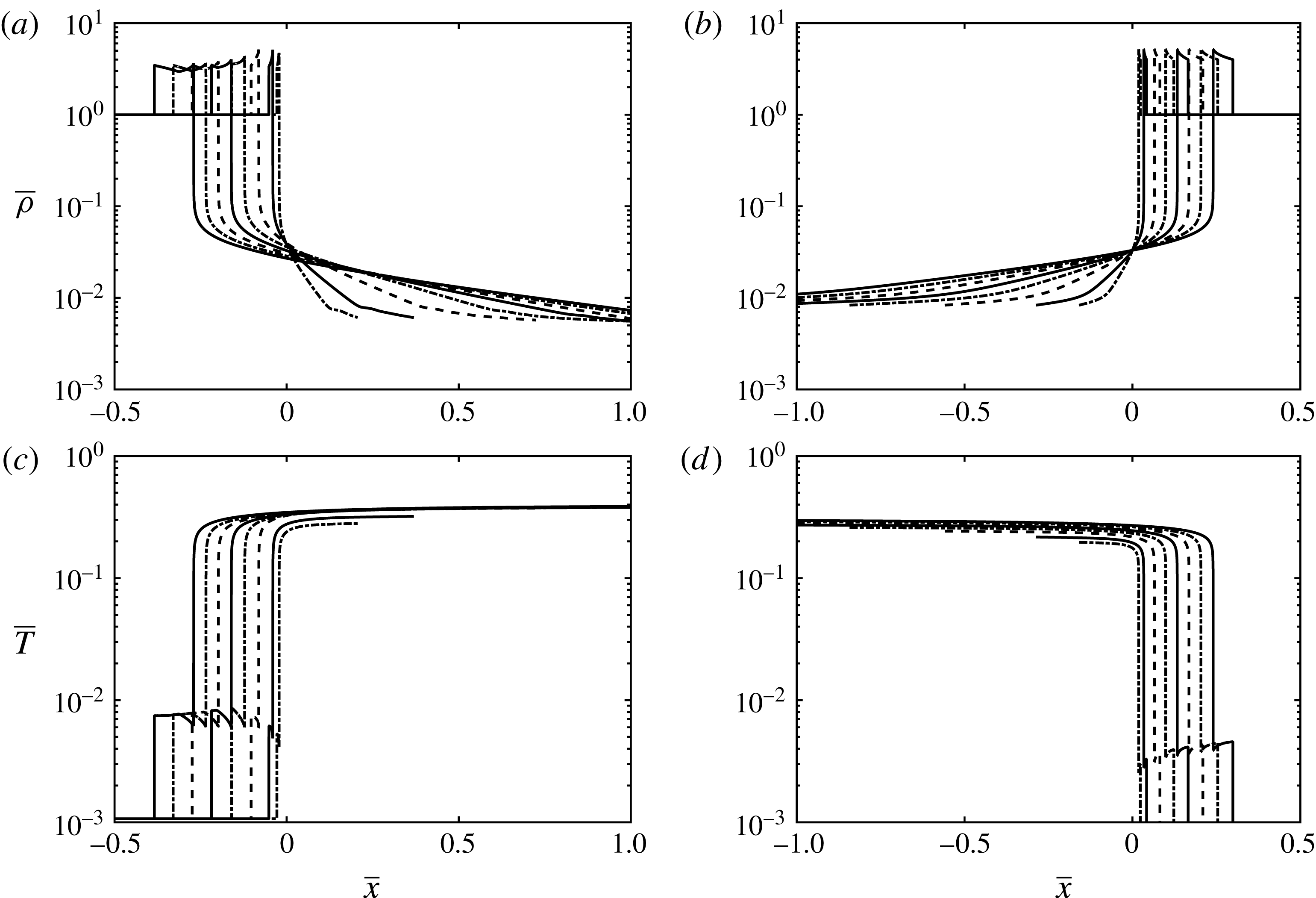
Early ablation of an ICF target. Time sequence of dimensionless spatial profiles in density (a,b) and temperature (c,d) corresponding to the X-ray-driven ablation of a spherical target outer shell. Results from a numerical simulation (a,c) of an implosion of the LMJ target (Saillard Reference Saillard2000, figure 1) surrounded by the hohlraum gas – with the radiation hydrodynamics code FCI2 (Buresi et al. Reference Buresi1986) in the radiation heat-conduction approximation – and from a particular solution (b,d, in mirror symmetry) belonging to the family of self-similar ablative waves described in this paper. The chosen time sequence samples the whole ‘foot’ duration of the hohlraum radiative temperature drive of the type given in Saillard (Reference Saillard2000, figure 5) which corresponds to an ablative-wave regime of the target outer shell flow. Despite the fact that, in the simulation, the target external boundary pressure and radiative flux do not follow the time power laws (3.4a,b ) of similarity solutions, nor does the material opacity reduce to a power law of the fluid density and temperature, the self-similar profiles reproduce the essential features of the ablative wave penetrating the target outer shell.

This overview of over 70 years of studies on radiative-wave flows highlights the central role that self-similar solutions of the gas dynamics equations with nonlinear heat conduction have repeatedly played in describing and understanding such flows. Indeed these solutions comprise the essential features – nonlinear heat conduction, compressibility and unsteadiness – as well as reproduce the structure of elementary flows driven by an external time-growing radiation source (figure 1). The rationale behind the present work builds on these facts. Sharing the point of view expressed in Marshak (Reference Marshak1958), we hold ablative self-similar solutions to be particular, yet realistic, instances of unsteady ablative flows driven by nonlinear heat conduction. Being able to numerically compute such solutions to a high accuracy (Gauthier et al. Reference Gauthier, Le Creurer, Abéguilé, Boudesocque-Dubois and Clarisse2005; Boudesocque-Dubois et al. Reference Boudesocque-Dubois, Lombard, Gauthier and Clarisse2013) allows us to obtain a trustworthy depiction of the mechanisms at work in these flows that is not blurred by numerical artefacts nor altered by additional modelling assumptions. A better understanding of ablative flows can then be expected from a detailed quantitative hydrodynamic analysis of these self-similar solutions. A further motivation is the hydrodynamic stability analysis of ablative flows for which this type of quantitative analysis is essential, as a preliminary step, for characterizing the background flow. The present study focuses on solutions obtained with the radiative conduction model of Kramers for a fully ionized gas (cf. Zel’dovich & Raizer Reference Zel’dovich and Raizer1967). In relation with ICF target implosions driven from rest by gas-filled hohlraum X-rays, boundary conditions are chosen to be specified in terms of heat flux and pressure, the latter giving the possibility of accounting for the mechanical action of the low-density gas filling the hohlraum. The relevant self-similar solutions, which are density invariant, may then display flow profiles typical of those of the early ablation of an ICF target by thermal radiation (figure 2). After introducing governing equations with initial and boundary conditions for the one-dimensional motion of a semi-infinite, initially homogeneous, fluid slab subject to time-varying external pressure and radiation (§ 2.1), the three dimensionless formulations of the equations of motion used for the present hydrodynamic analysis are given (§ 2.2). Density-invariant self-similar solutions obtained under the approximation of a non-isothermal bounding shock wave are then explored (§ 3) leading to an extensive set of high accuracy numerical solutions. A quantitative analysis of the corresponding radiative ablation waves is then conducted in terms of standard hydrodynamic characteristic numbers (Mach, Péclet, stratification and Froude numbers) supplemented by the main flow region relative lengths, along with an examination of the low Mach number approximation often invoked in hydrodynamic stability analyses of ablation flows in ICF (§ 4.1 and appendix B of the supplementary material). This analysis is supplemented by an investigation of linear-wave propagation in compressible inhomogeneous ablative flows with applications to self-similar solutions that are representative of flow regimes described by the present set of radiative ablation waves (§ 4.2).
2 Governing equations and dimensionless formulations
2.1 One-dimensional Euler equations with nonlinear heat conduction
Consider the one-dimensional motion, in slab symmetry, of an inviscid heat conducting compressible fluid along the
 $x$
-axis of a Cartesian coordinate system
 $(x,y,z)$
. The equations of motion can be written, with the help of the Lagrangian coordinate
 $m$
such that
 $\text{d}m=\unicode[STIX]{x1D70C}\,\text{d}x$
, as
 $$\begin{eqnarray}\displaystyle & \displaystyle \frac{\unicode[STIX]{x2202}}{\unicode[STIX]{x2202}t}\left(\frac{1}{\unicode[STIX]{x1D70C}}\right)-\frac{\unicode[STIX]{x2202}v_{x}}{\unicode[STIX]{x2202}m}=0, & \displaystyle\end{eqnarray}$$
 $$\begin{eqnarray}\displaystyle & \displaystyle \frac{\unicode[STIX]{x2202}v_{x}}{\unicode[STIX]{x2202}t}+\frac{\unicode[STIX]{x2202}p}{\unicode[STIX]{x2202}m}=0, & \displaystyle\end{eqnarray}$$
 $$\begin{eqnarray}\displaystyle & \displaystyle \frac{\unicode[STIX]{x2202}}{\unicode[STIX]{x2202}t}\left(\frac{1}{2}v_{x}^{2}+{\mathcal{E}}\right)+\frac{\unicode[STIX]{x2202}}{\unicode[STIX]{x2202}m}\left(pv_{x}+\unicode[STIX]{x1D711}_{x}\right)=0, & \displaystyle\end{eqnarray}$$
 $\unicode[STIX]{x1D70C}$
and
 $p$
are the fluid density and pressure,
 $v_{x}$
is the fluid velocity,
 ${\mathcal{E}}$
is the fluid specific internal energy and
 $\unicode[STIX]{x1D711}_{x}$
is the heat flux. Assuming a polytropic equation of state,
 $$\begin{eqnarray}p=R\,\unicode[STIX]{x1D70C}\,T,\quad {\mathcal{E}}=\text{C}_{v}\,T,\quad \text{with}~\text{C}_{v}=R/(\unicode[STIX]{x1D6FE}-1),\end{eqnarray}$$
where
 $R$
is the gas constant and
 $\unicode[STIX]{x1D6FE}$
the fluid adiabatic exponent, and a nonlinear heat conduction of the form
 $$\begin{eqnarray}\unicode[STIX]{x1D711}_{x}=-\unicode[STIX]{x1D70C}\,\unicode[STIX]{x1D705}(\unicode[STIX]{x1D70C},T)\,\frac{\unicode[STIX]{x2202}T}{\unicode[STIX]{x2202}m},\quad \text{with}~\unicode[STIX]{x1D705}(\unicode[STIX]{x1D70C},T)=\unicode[STIX]{x1D705}_{0}\left(\frac{\unicode[STIX]{x1D70C}_{0}}{\unicode[STIX]{x1D70C}}\right)^{\unicode[STIX]{x1D707}}\left(\frac{T}{T_{0}}\right)^{\unicode[STIX]{x1D708}},~\unicode[STIX]{x1D705}_{0}>0,~\unicode[STIX]{x1D707}\geqslant 0,~\unicode[STIX]{x1D708}>0,\end{eqnarray}$$
where
 $\unicode[STIX]{x1D70C}_{0}$
and
 $T_{0}$
are homogenization constants, the equations in (2.1) with expressions (2.2) and (2.3) constitute a system of quasilinear second-order partial differential equations (PDEs) with quadratic terms in first-order derivatives. The configuration of a semi-infinite slab of fluid, initially homogeneous and at rest, set into motion under the combined action of some external heat source and pressure, can be addressed by considering the initial conditions
 $$\begin{eqnarray}\unicode[STIX]{x1D70C}(m,0)=\unicode[STIX]{x1D70C}_{I},\quad v_{x}(m,0)=0,\quad T(m,0)=T_{I},\quad \text{for }m\geqslant 0,\end{eqnarray}$$
where
 $\unicode[STIX]{x1D70C}_{I}$
and
 $T_{I}$
are constants, along with the boundary conditions
 $$\begin{eqnarray}p(0,t)=p^{\unicode[STIX]{x1D6E4}}(t),\quad \unicode[STIX]{x1D711}_{x}(0,t)=\unicode[STIX]{x1D711}_{x}^{\unicode[STIX]{x1D6E4}}(t),\quad \text{for }t\geqslant 0.\end{eqnarray}$$
2.2 Dimensionless formulations
Introducing for any quantity
 $q$
, the notation
 $q=q_{\star }\,\bar{q}$
where
 $q_{\star }$
denotes the scale of
 $q$
and
 $\bar{q}$
its dimensionless counterpart, along with the relation
 $q(m,t)\equiv q_{\star }\,\bar{q}(\bar{m},\bar{t})$
for dependent variables, the dimensionless form of (2.1) is written as
 $$\begin{eqnarray}\displaystyle & \displaystyle \frac{\unicode[STIX]{x2202}}{\unicode[STIX]{x2202}\bar{t}}\left(\frac{1}{\bar{\unicode[STIX]{x1D70C}}}\right)-\unicode[STIX]{x1D6F4}_{1}\,\frac{\unicode[STIX]{x2202}\bar{v}_{x}}{\unicode[STIX]{x2202}\bar{m}}=0, & \displaystyle\end{eqnarray}$$
 $$\begin{eqnarray}\displaystyle & \displaystyle \frac{\unicode[STIX]{x2202}\bar{v}_{x}}{\unicode[STIX]{x2202}\bar{t}}+\unicode[STIX]{x1D6F4}_{2}\,\frac{\unicode[STIX]{x2202}\bar{p}}{\unicode[STIX]{x2202}\bar{m}}=0, & \displaystyle\end{eqnarray}$$
 $$\begin{eqnarray}\displaystyle & \displaystyle \frac{\unicode[STIX]{x2202}}{\unicode[STIX]{x2202}\bar{t}}\left(\frac{1}{2}\,\bar{v}_{x}^{2}+\unicode[STIX]{x1D6F4}_{3}\,\bar{T}\right)+\frac{\unicode[STIX]{x2202}}{\unicode[STIX]{x2202}\bar{m}}\left(\unicode[STIX]{x1D6F4}_{2}\,\bar{p}\,\bar{v}_{x}+\unicode[STIX]{x1D6F4}_{4}\,\bar{\unicode[STIX]{x1D711}}_{x}\right)=0, & \displaystyle\end{eqnarray}$$
 $$\begin{eqnarray}\bar{p}=\unicode[STIX]{x1D6F4}_{6}\,\bar{\unicode[STIX]{x1D70C}}\,\bar{T},\end{eqnarray}$$
in place of (2.2), and
 $$\begin{eqnarray}\bar{\unicode[STIX]{x1D711}}_{x}=-\unicode[STIX]{x1D6F4}_{5}\,\bar{\unicode[STIX]{x1D70C}}\,\bar{\unicode[STIX]{x1D705}}(\bar{\unicode[STIX]{x1D70C}},\bar{T})\,\frac{\unicode[STIX]{x2202}\bar{T}}{\unicode[STIX]{x2202}\bar{m}},\quad \text{with}~\bar{\unicode[STIX]{x1D705}}(\bar{\unicode[STIX]{x1D70C}},\bar{T})=\bar{\unicode[STIX]{x1D70C}}^{-\unicode[STIX]{x1D707}}\,\bar{T}^{\unicode[STIX]{x1D708}},\end{eqnarray}$$
for (2.3). The dimensionless combinations
 $\unicode[STIX]{x1D6F4}_{i}$
,
 $i=1\ldots 6$
, involved in these equations, are given, in terms of the flow variable scales, by the expressions
 $$\begin{eqnarray}\left.\begin{array}{@{}c@{}}\unicode[STIX]{x1D6F4}_{1}=t_{\star }\,\unicode[STIX]{x1D70C}_{\star }\,v_{\star }\,m_{\star }^{-1},\quad \unicode[STIX]{x1D6F4}_{2}=t_{\star }\,p_{\star }\,v_{\star }^{-1}\,m_{\star }^{-1},\quad \unicode[STIX]{x1D6F4}_{3}=\text{C}_{v}T_{\star }v_{\star }^{-2},\\ \unicode[STIX]{x1D6F4}_{4}=t_{\star }\,\unicode[STIX]{x1D711}_{\star }\,v_{\star }^{-2}\,m_{\star }^{-1},\quad \unicode[STIX]{x1D6F4}_{5}=\unicode[STIX]{x1D705}_{\star }\,\unicode[STIX]{x1D70C}_{\star }\,T_{\star }\,\unicode[STIX]{x1D711}_{\star }^{-1}\,m_{\star }^{-1},\quad \unicode[STIX]{x1D6F4}_{6}=R\,\unicode[STIX]{x1D70C}_{\star }\,T_{\star }\,p_{\star }^{-1},\end{array}\right\}\end{eqnarray}$$
where, for convenience, the notation
 $$\begin{eqnarray}\unicode[STIX]{x1D705}_{\star }=\unicode[STIX]{x1D705}(\unicode[STIX]{x1D70C}_{\star },T_{\star })=\unicode[STIX]{x1D705}_{0}(\unicode[STIX]{x1D70C}_{0}/\unicode[STIX]{x1D70C}_{\star })^{\unicode[STIX]{x1D707}}(T_{\star }/T_{0})^{\unicode[STIX]{x1D708}},\end{eqnarray}$$
has been introduced. We note that
 $\unicode[STIX]{x1D70C}_{0}$
and
 $T_{0}$
may be chosen arbitrarily and independently of the respective scales
 $\unicode[STIX]{x1D70C}_{\star }$
and
 $T_{\star }$
. Dimensionless forms of the initial conditions (2.4) and boundary conditions (2.5) come as, respectively,
 $$\begin{eqnarray}\bar{\unicode[STIX]{x1D70C}}(\bar{m},0)=\unicode[STIX]{x1D70C}_{I}/\unicode[STIX]{x1D70C}_{\star },\quad \bar{v}_{x}(\bar{m},0)=0,\quad \bar{T}(\bar{m},0)=T_{I}/T_{\star },\quad \text{for }\bar{m}\geqslant 0,\end{eqnarray}$$
and
 $$\begin{eqnarray}\bar{p}(0,\bar{t})=p^{\unicode[STIX]{x1D6E4}}(t_{\star }\bar{t})/p_{\star },\quad \bar{\unicode[STIX]{x1D711}}_{x}(0,\bar{t})=\unicode[STIX]{x1D711}_{x}^{\unicode[STIX]{x1D6E4}}(t_{\star }\bar{t})/\unicode[STIX]{x1D711}_{\star },\quad \text{for }\bar{t}\geqslant 0.\end{eqnarray}$$
The problem defined by (2.1)–(2.3) depends on four independent units which we take to be the units of mass,
 $\unicode[STIX]{x1D614}$
, of length,
 $\unicode[STIX]{x1D62D}$
, of time,
 $\unicode[STIX]{x1D635}$
, and of temperature,
 $\unicode[STIX]{x1D61B}$
. The actual procedure for determining the dimensionless combinations
 $\unicode[STIX]{x1D6F4}_{i}$
that define a given dimensionless formulation (2.6)–(2.8), follows the systematic approach presented in Langhaar (Reference Langhaar1951) and which makes use of the dimensional matrix of the problem. The flow described by the set of equations (2.1)–(2.5), is governed – the conductivity law exponents
 $\unicode[STIX]{x1D707}$
and
 $\unicode[STIX]{x1D708}$
being given – by the fluid physical parameters
 $\unicode[STIX]{x1D6FE}$
,
 $R$
,
 $\unicode[STIX]{x1D705}_{0}$
, the initial fluid density
 $\unicode[STIX]{x1D70C}_{I}$
and some reference values of the boundary pressure and heat flux, say
 $$\begin{eqnarray}p_{\unicode[STIX]{x1D6E4}}=p^{\unicode[STIX]{x1D6E4}}(t_{\star }),\quad \unicode[STIX]{x1D711}_{\unicode[STIX]{x1D6E4}}=\unicode[STIX]{x1D711}_{x}^{\unicode[STIX]{x1D6E4}}(t_{\star }).\end{eqnarray}$$
Three dimensionless formulations of these equations are considered for the present goal of analysing ablation flows.
2.2.1
 $({\mathcal{B}}_{p},{\mathcal{B}}_{\unicode[STIX]{x1D711}})$
-formulation

The first dimensionless formulation that we use is obtained upon introducing a reference time
 $t_{c}$
as an additional governing physical parameter (Abéguilé et al.
Reference Abéguilé, Boudesocque-Dubois, Clarisse, Gauthier and Saillard2006; Clarisse, Boudesocque-Dubois & Gauthier Reference Clarisse, Boudesocque-Dubois and Gauthier2008). We have then three dimensionless governing parameters
 $\unicode[STIX]{x1D6FD}_{1}$
,
 $\unicode[STIX]{x1D6FD}_{2}$
,
 $\unicode[STIX]{x1D6FD}_{3}$
(table 1
a.i) that, aside from
 $\unicode[STIX]{x1D6FD}_{1}$
, we ascribe to the boundary-condition parameters
 $$\begin{eqnarray}C_{\bar{p}}^{\unicode[STIX]{x1D6E4}}=p_{\unicode[STIX]{x1D6E4}}/p_{\star },\quad C_{\bar{\unicode[STIX]{x1D711}}}^{\unicode[STIX]{x1D6E4}}=\unicode[STIX]{x1D711}_{\unicode[STIX]{x1D6E4}}/\unicode[STIX]{x1D711}_{\star },\end{eqnarray}$$
by imposing the dimensionless combinations
 $\unicode[STIX]{x1D6F4}_{i}$
,
 $i\neq 3$
, in (2.6)–(2.8) to be of constant and equal weights (table 1
a.iii). Setting in addition
 $\unicode[STIX]{x1D70C}_{\star }=\unicode[STIX]{x1D70C}_{I}$
and
 $t_{\star }=t_{c}$
for the density and time scales, and for the sake of simplicity
 $$\begin{eqnarray}\unicode[STIX]{x1D70C}_{0}=\unicode[STIX]{x1D70C}_{\star },\quad T_{0}=T_{\star },\end{eqnarray}$$
in (2.10), leads to the expressions of table 1(a.ii) for the remaining flow variable scales
 $q_{\star }$
, and of table 1(a.iii) for the remaining dimensionless combination
 $\unicode[STIX]{x1D6F4}_{3}$
, the initial condition parameter
 $C_{\bar{\unicode[STIX]{x1D70C}}}^{I}\equiv \unicode[STIX]{x1D70C}_{I}/\unicode[STIX]{x1D70C}_{\star }$
and the boundary-condition parameters
 $C_{\bar{p}}^{\unicode[STIX]{x1D6E4}}$
,
 $C_{\bar{\unicode[STIX]{x1D711}}}^{\unicode[STIX]{x1D6E4}}$
. From table 1(a.iii), the resulting form of system (2.6)–(2.8), or
 $({\mathcal{B}}_{p},{\mathcal{B}}_{\unicode[STIX]{x1D711}})$
-formulation, reads
 $$\begin{eqnarray}\left.\begin{array}{@{}c@{}}\displaystyle \frac{\unicode[STIX]{x2202}}{\unicode[STIX]{x2202}\bar{t}}\left(\frac{1}{\bar{\unicode[STIX]{x1D70C}}}\right)-\frac{\unicode[STIX]{x2202}\bar{v}_{x}}{\unicode[STIX]{x2202}\bar{m}}=0,\\ \displaystyle \frac{\unicode[STIX]{x2202}\bar{v}_{x}}{\unicode[STIX]{x2202}\bar{t}}+\frac{\unicode[STIX]{x2202}\bar{p}}{\unicode[STIX]{x2202}\bar{m}}=0,\\ \displaystyle \frac{\unicode[STIX]{x2202}}{\unicode[STIX]{x2202}\bar{t}}\left(\frac{1}{2}\bar{v}_{x}^{2}+\frac{\bar{T}}{\unicode[STIX]{x1D6FE}-1}\right)+\frac{\unicode[STIX]{x2202}}{\unicode[STIX]{x2202}\bar{m}}\left(\bar{p}\bar{v}_{x}+\bar{\unicode[STIX]{x1D711}}_{x}\right)=0,\end{array}\right\}\end{eqnarray}$$
with the equation-of-state relation
 $$\begin{eqnarray}\bar{p}=\bar{\unicode[STIX]{x1D70C}}\,\bar{T},\end{eqnarray}$$
and the heat-flux expression
 $$\begin{eqnarray}\bar{\unicode[STIX]{x1D711}}_{x}=-\bar{\unicode[STIX]{x1D70C}}\,\bar{\unicode[STIX]{x1D705}}(\bar{\unicode[STIX]{x1D70C}},\bar{T})\,\frac{\unicode[STIX]{x2202}\bar{T}}{\unicode[STIX]{x2202}\bar{m}},\end{eqnarray}$$
while the initial and boundary conditions follow readily from (2.11), (2.12). We note that this dimensionless formulation can also be established upon using, in place of
 $t_{c}$
, a reference velocity (cf. Samarskiĭ et al.
Reference Samarskiĭ, Kurdyumov and Volosevich1965; Boudesocque-Dubois et al.
Reference Boudesocque-Dubois, Gauthier and Clarisse2008) or a reference temperature (Boudesocque-Dubois Reference Boudesocque-Dubois2000).
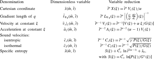
Defining parameters for the three chosen dimensionless formulations of (2.1)–(2.5):
 $({\mathcal{B}}_{p},{\mathcal{B}}_{\unicode[STIX]{x1D711}})$
-formulation (a);
 $({\mathcal{M}},{\mathcal{P}}\mathit{e})$
-formulation (b);
 $(\mathit{M}^{\prime },\mathit{Fr}^{\prime },\mathit{Pe}^{\prime })$
-formulation (c). In each case, (i) the expressions of the dimensionless governing parameters along with the chosen definitions (

 $\unicode[STIX]{x1D6F4}_{i}$
(2.9), (2.24), and initial/boundary-condition parameters are given. The corresponding dimensionless forms of (2.1)–(2.5) follow from substituting into (2.6) (alternatively (2.23)), (2.7), (2.8), (2.11), (2.12) the entry values given in (a.iii), (b.iii) (alternatively c.iii).

2.2.2
$({\mathcal{M}},{\mathcal{P}}\mathit{e})$
-formulation

With the same set of physical governing parameters, we introduce a dimensionless formulation of the initial and boundary value problem (IBVP) (2.1)–(2.5) where now the dimensionless driving parameters of the problem are coefficients of (2.6) instead of being the boundary-condition parameters (2.14). The set of dimensionless governing parameters being identical to that of the preceding formulation (cf. table 1
b.i), this new formulation is achieved by: (i) setting
 $C_{\bar{p}}^{\unicode[STIX]{x1D6E4}}=1$
and
 $C_{\bar{\unicode[STIX]{x1D711}}}^{\unicode[STIX]{x1D6E4}}=1$
; (ii) choosing to leave invariant the mass conservation equation (2.6a
) and the equation of state (2.7) – in effect
 $\unicode[STIX]{x1D6F4}_{1}=1$
and
 $\unicode[STIX]{x1D6F4}_{6}=1$
– while retaining the density and time scales of table 1(a.ii); (iii) keeping the choice made in (2.15); (iv) defining the velocity scale to be
 $v_{\star }=\unicode[STIX]{x1D711}_{\unicode[STIX]{x1D6E4}}/p_{\unicode[STIX]{x1D6E4}}$
. The remaining flow variable scales ensue as in table 1(b.ii) while the dimensionless combinations
 $\unicode[STIX]{x1D6F4}_{i}$
,
 $i=2\ldots 5$
, are expressed (table 1
b.iii) in terms of a ‘Mach number scale’
 $$\begin{eqnarray}{\mathcal{M}}=v_{\star }/c_{c},\quad \text{with}~c_{c}=\sqrt{\unicode[STIX]{x1D6FE}\,p_{\unicode[STIX]{x1D6E4}}/\unicode[STIX]{x1D70C}_{I}},\end{eqnarray}$$
and a ‘Péclet number scale’
 $$\begin{eqnarray}{\mathcal{P}}\mathit{e}=\frac{t_{c}\,v_{\star }^{2}}{\unicode[STIX]{x1D705}_{0}/\unicode[STIX]{x1D70C}_{I}\,\text{C}_{p}}=\frac{\unicode[STIX]{x1D6FE}}{\unicode[STIX]{x1D6FE}-1}\,R\,\unicode[STIX]{x1D705}_{0}^{-1}\,\unicode[STIX]{x1D70C}_{I}\,t_{c}\,v_{\star }^{2},\end{eqnarray}$$
built from the length scale
 $t_{c}\,v_{\star }$
and the diffusivity scale
 $\unicode[STIX]{x1D705}_{0}/\unicode[STIX]{x1D70C}_{I}\,\text{C}_{p}=(\unicode[STIX]{x1D6FE}-1)\,\unicode[STIX]{x1D705}_{0}/\unicode[STIX]{x1D6FE}\,R\,\unicode[STIX]{x1D70C}_{I}$
. The corresponding form, or
 $({\mathcal{M}},{\mathcal{P}}\mathit{e})$
-formulation, of system (2.6)–(2.8) follows as
 $$\begin{eqnarray}\left.\begin{array}{@{}c@{}}\displaystyle \frac{\unicode[STIX]{x2202}}{\unicode[STIX]{x2202}\bar{t}}\left(\frac{1}{\bar{\unicode[STIX]{x1D70C}}}\right)-\frac{\unicode[STIX]{x2202}\bar{v}_{x}}{\unicode[STIX]{x2202}\bar{m}}=0,\\ \displaystyle \frac{\unicode[STIX]{x2202}\bar{v}_{x}}{\unicode[STIX]{x2202}\bar{t}}+\frac{1}{\unicode[STIX]{x1D6FE}\,{\mathcal{M}}^{2}}\,\frac{\unicode[STIX]{x2202}\bar{p}}{\unicode[STIX]{x2202}\bar{m}}=0,\\ \displaystyle \frac{\unicode[STIX]{x2202}}{\unicode[STIX]{x2202}\bar{t}}\left(\frac{1}{2}\bar{v}_{x}^{2}+\frac{1}{\unicode[STIX]{x1D6FE}\,{\mathcal{M}}^{2}}\,\frac{\bar{T}}{\unicode[STIX]{x1D6FE}-1}\right)+\frac{1}{\unicode[STIX]{x1D6FE}\,{\mathcal{M}}^{2}}\,\frac{\unicode[STIX]{x2202}}{\unicode[STIX]{x2202}\bar{m}}\left(\bar{p}\bar{v}_{x}+\bar{\unicode[STIX]{x1D711}}_{x}\right)=0,\end{array}\right\}\end{eqnarray}$$
with the equation-of-state relation (2.17), the heat-flux expression
 $$\begin{eqnarray}\bar{\unicode[STIX]{x1D711}}_{x}=-\frac{\unicode[STIX]{x1D6FE}}{(\unicode[STIX]{x1D6FE}-1)\,{\mathcal{P}}\mathit{e}}\,\bar{\unicode[STIX]{x1D70C}}^{1-\unicode[STIX]{x1D707}}\,\bar{T}^{\unicode[STIX]{x1D708}}\,\frac{\unicode[STIX]{x2202}\bar{T}}{\unicode[STIX]{x2202}\bar{m}},\end{eqnarray}$$
and initial and boundary conditions resulting from (2.11), (2.12) with the values of
 $C_{\bar{\unicode[STIX]{x1D70C}}}^{I}$
,
 $p_{\star }$
,
 $\unicode[STIX]{x1D711}_{\star }$
given in table 1(b). Upon replacing
 $\bar{\unicode[STIX]{x1D711}}_{x}$
by its expression (2.22), system (2.21) takes the standard form of the dimensionless Euler equations written in terms of Mach and Péclet numbers for a nonlinear heat conductivity of the type (2.3).
2.2.3
$(\mathit{M}^{\prime },\mathit{Fr}^{\prime },\mathit{Pe}^{\prime })$
-formulation

A third dimensionless formulation of the IBVP (2.1)–(2.5) is introduced with the aim of obtaining a low Mach number approximation of the Euler equations with heat conduction (Paolucci Reference Paolucci1982) in the context of ablative flows. The equations of motion (2.1) rewritten in a non-inertial reference frame moving, with respect to the laboratory frame, with the velocity
 $\boldsymbol{v}^{\unicode[STIX]{x1D65A}}=v^{\unicode[STIX]{x1D626}}(t)\,\boldsymbol{e}_{x}$
and acceleration
 $\boldsymbol{a}^{\unicode[STIX]{x1D65A}}=a^{\unicode[STIX]{x1D626}}(t)\,\boldsymbol{e}_{x}\equiv (\text{d}v^{\unicode[STIX]{x1D626}}(t)/\text{d}t)\,\boldsymbol{e}_{x}$
, yield the general dimensionless form

where
 $\bar{v}_{x}^{\prime }=(v_{x}-v^{\unicode[STIX]{x1D626}})/v_{\star }$
is the dimensionless fluid velocity in the moving frame, and
 $$\begin{eqnarray}\unicode[STIX]{x1D6F4}_{7}=t_{\star }\,a_{\star }\,v_{\star }^{-1}.\end{eqnarray}$$
A most versatile form of (2.23) is built from the three physical governing parameters of the problem
 $\unicode[STIX]{x1D6FE}$
,
 $\unicode[STIX]{x1D705}_{0}$
,
 $R$
, supplemented here by some reference values of density,
 $\unicode[STIX]{x1D70C}_{c}$
, temperature,
 $T_{c}$
, length,
 $\ell _{c}$
, relative fluid velocity,
 $v_{c}^{\prime }$
, and frame acceleration,
 $a_{c}^{\unicode[STIX]{x1D626}}$
. We have then four dimensionless governing parameters (table 1
c.i) and the retained dimensionless formulation follows from: (i) choosing to leave invariant the mass conservation equation (2.6a
), the equation of state (2.7), the heat-flux expression (2.8) as in § 2.2.1 – in effect
 $\unicode[STIX]{x1D6F4}_{1}=\unicode[STIX]{x1D6F4}_{5}=\unicode[STIX]{x1D6F4}_{6}=1$
; (ii) setting the scales for the density, velocity, temperature, time and acceleration to be respectively
 $\unicode[STIX]{x1D70C}_{\star }=\unicode[STIX]{x1D70C}_{c}$
,
 $v_{\star }=v_{c}^{\prime }$
,
 $T_{\star }=T_{c}$
,
 $t_{\star }=\ell _{c}/v_{c}^{\prime }$
and
 $a_{\star }=a_{c}^{\unicode[STIX]{x1D626}}$
. The remaining flow variable scales (table 1
c.ii) and dimensionless combinations (table 1
c.iii) lead to the following form of system (2.23), or
 $(\mathit{M}^{\prime },\mathit{Fr}^{\prime },\mathit{Pe}^{\prime })$
-formulation,

with the equation-of-state relation (2.17), the nonlinear heat-flux expression (2.18), and the Mach, Péclet, Froude number expressions
 $$\begin{eqnarray}\mathit{M}^{\prime }=\frac{v_{c}^{\prime }}{\sqrt{\unicode[STIX]{x1D6FE}\,R\,T_{c}}},\quad \mathit{Pe}^{\prime }=\frac{\ell _{c}\,v_{c}^{\prime }}{\unicode[STIX]{x1D705}_{\star }/\text{C}_{p}\,\unicode[STIX]{x1D70C}_{c}},\quad \mathit{Fr}^{\prime }=\frac{v_{c}^{\prime }}{\sqrt{a_{c}^{\unicode[STIX]{x1D626}}\,\ell _{c}}}.\end{eqnarray}$$
The above Péclet number definition as well as the expressions (table 1
c) for
 $\unicode[STIX]{x1D711}_{\star }$
and
 $C_{\bar{\unicode[STIX]{x1D711}}}^{\unicode[STIX]{x1D6E4}}$
involve – contrary to the previous dimensionless formulations of §§ 2.2.1 and 2.2.2 – the quantity
 $\unicode[STIX]{x1D705}_{\star }$
defined by (2.10), since the homogenization constants
 $\unicode[STIX]{x1D70C}_{0}$
and
 $T_{0}$
are left unspecified. System (2.25) is the standard dimensionless formulation (e.g. Paolucci Reference Paolucci1982), in terms of Mach, Froude and Péclet numbers, of the Euler equations with heat conduction in a non-inertial reference frame.
3 Invariant-density self-similar solutions of radiative ablation
Independently of any particular choice of dimensionless formulation for the system of equations (2.1)–(2.3), a similarity transformations of the initial and boundary value problem (2.6)–(2.8), (2.11), (2.12) can be achieved (e.g. Marshak Reference Marshak1958; Brun et al. Reference Brun, Dautray, Delobeau, Patou, Perrot, Reisse, Sitt, Watteau, Schwarz and Hora1977; Sanz et al. Reference Sanz, Piriz and Tomasel1992). Details can be found in Boudesocque-Dubois et al. (Reference Boudesocque-Dubois, Gauthier and Clarisse2008), Clarisse et al. (Reference Clarisse, Boudesocque-Dubois and Gauthier2008) and we only recall here the main results. Similarity transformations that are compatible with the initial and boundary conditions (2.11), (2.12), constitute a one parameter group and leave invariant the density. The reduced independent variable is
 $$\begin{eqnarray}\unicode[STIX]{x1D709}=\bar{m}\,\bar{t}^{-\unicode[STIX]{x1D6FC}},\quad \text{with}~\unicode[STIX]{x1D6FC}=\frac{2\unicode[STIX]{x1D708}-1}{2\unicode[STIX]{x1D708}-2},\end{eqnarray}$$
and the main variable reduction relations are
 $$\begin{eqnarray}\left.\begin{array}{@{}c@{}}\bar{\unicode[STIX]{x1D70C}}(\bar{m},\bar{t})=G(\unicode[STIX]{x1D709}),\quad \bar{v}_{x}(\bar{m},\bar{t})=\bar{t}^{\unicode[STIX]{x1D6FC}-1}\,V(\unicode[STIX]{x1D709}),\\ \bar{T}(\bar{m},\bar{t})=\bar{t}^{2(\unicode[STIX]{x1D6FC}-1)}\,\unicode[STIX]{x1D6E9}(\unicode[STIX]{x1D709}),\quad \bar{\unicode[STIX]{x1D711}}_{x}(\bar{m},\bar{t})=\bar{t}^{3(\unicode[STIX]{x1D6FC}-1)}\,\unicode[STIX]{x1D6F7}(\unicode[STIX]{x1D709}),\end{array}\right\}\end{eqnarray}$$
provided that initial and boundary conditions (2.11), (2.12), are of the form
 $$\begin{eqnarray}\bar{\unicode[STIX]{x1D70C}}(\bar{m},0)=C_{\bar{\unicode[STIX]{x1D70C}}}^{I},\quad \bar{v}_{x}(\bar{m},0)=0,\quad \bar{T}(\bar{m},0)=0,\quad \text{for }\bar{m}\geqslant 0,\end{eqnarray}$$
 $$\begin{eqnarray}\bar{p}(0,\bar{t})=C_{\bar{p}}^{\unicode[STIX]{x1D6E4}}\,\bar{t}^{2(\unicode[STIX]{x1D6FC}-1)},\quad \bar{\unicode[STIX]{x1D711}}_{x}(0,\bar{t})=C_{\bar{\unicode[STIX]{x1D711}}}^{\unicode[STIX]{x1D6E4}}\,\bar{t}^{3(\unicode[STIX]{x1D6FC}-1)},\quad \text{for }\bar{t}\geqslant 0.\end{eqnarray}$$
The reduced form of the IBVP (2.6)–(2.8), (3.3), (3.4) is then
 $$\begin{eqnarray}\left.\begin{array}{@{}c@{}}\displaystyle \unicode[STIX]{x1D6FC}\unicode[STIX]{x1D709}\,\frac{\text{d}}{\text{d}\unicode[STIX]{x1D709}}\left(\frac{1}{G}\right)+\unicode[STIX]{x1D6F4}_{1}\,\frac{\text{d}V}{\text{d}\unicode[STIX]{x1D709}}=0,\\ \displaystyle \unicode[STIX]{x1D6FC}\unicode[STIX]{x1D709}\,\frac{\text{d}V}{\text{d}\unicode[STIX]{x1D709}}-\unicode[STIX]{x1D6F4}_{2}\,\unicode[STIX]{x1D6F4}_{6}\,\frac{\text{d}G\,\unicode[STIX]{x1D6E9}}{\text{d}\unicode[STIX]{x1D709}}=\left(\unicode[STIX]{x1D6FC}-1\right)V,\\ \displaystyle \unicode[STIX]{x1D6F4}_{5}\,G^{1-\unicode[STIX]{x1D707}}\,\unicode[STIX]{x1D6E9}^{\unicode[STIX]{x1D708}}\,\frac{\text{d}\unicode[STIX]{x1D6E9}}{\text{d}\unicode[STIX]{x1D709}}=-\unicode[STIX]{x1D6F7},\\ \displaystyle \unicode[STIX]{x1D6FC}\unicode[STIX]{x1D709}\,\frac{\text{d}}{\text{d}\unicode[STIX]{x1D709}}\left(\frac{V^{2}}{2}+\unicode[STIX]{x1D6F4}_{3}\,\unicode[STIX]{x1D6E9}\right)-\unicode[STIX]{x1D6F4}_{2}\,\unicode[STIX]{x1D6F4}_{6}\,\frac{\text{d}G\,\unicode[STIX]{x1D6E9}\,V}{\text{d}\unicode[STIX]{x1D709}}-\unicode[STIX]{x1D6F4}_{4}\,\frac{\text{d}\unicode[STIX]{x1D6F7}}{\text{d}\unicode[STIX]{x1D709}}=2(\unicode[STIX]{x1D6FC}-1)\left(\frac{V^{2}}{2}+\unicode[STIX]{x1D6F4}_{3}\,\unicode[STIX]{x1D6E9}\right),\end{array}\right\}\end{eqnarray}$$
with boundary conditions given, from (3.3), by
 $$\begin{eqnarray}G\rightarrow C_{\bar{\unicode[STIX]{x1D70C}}}^{I},\quad V\rightarrow 0,\quad \unicode[STIX]{x1D6E9}\rightarrow 0,\quad \unicode[STIX]{x1D6F7}\rightarrow 0,\quad \text{as }\unicode[STIX]{x1D709}\rightarrow +\infty ,\end{eqnarray}$$
and, from (3.4), by
 $$\begin{eqnarray}P(0)=\unicode[STIX]{x1D6F4}_{6}\,G(0)\,\unicode[STIX]{x1D6E9}(0)=C_{\bar{p}}^{\unicode[STIX]{x1D6E4}},\quad \unicode[STIX]{x1D6F7}(0)=C_{\bar{\unicode[STIX]{x1D711}}}^{\unicode[STIX]{x1D6E4}}.\end{eqnarray}$$
Singularities
The system of ODEs (3.5) presents three singularities (cf. Reinicke & Meyer-ter-Vehn, Reference Reinicke and Meyer-ter-Vehn1991, for a detailed analysis of a similar system), namely:
(i)
$\unicode[STIX]{x1D6E5}(\unicode[STIX]{x1D709})=\unicode[STIX]{x1D6FC}^{2}\,\unicode[STIX]{x1D709}^{2}-\unicode[STIX]{x1D6F4}_{1}\,\unicode[STIX]{x1D6F4}_{2}\,\unicode[STIX]{x1D6F4}_{6}\,G^{2}\,\unicode[STIX]{x1D6E9}=0$
: isothermal sonic point. The locus
$\unicode[STIX]{x1D709}_{sp}$
:
$\unicode[STIX]{x1D6FC}^{2}\,\unicode[STIX]{x1D709}_{sp}^{2}=\unicode[STIX]{x1D6F4}_{1}\,\unicode[STIX]{x1D6F4}_{2}\,\unicode[STIX]{x1D6F4}_{6}\,G^{2}\,\unicode[STIX]{x1D6E9}$
, corresponds to the characteristic curve
$\text{d}\bar{m}/\text{d}\bar{t}=\bar{\unicode[STIX]{x1D70C}}\,\bar{c}_{T}$
of the
$(\bar{m},\bar{t})$
-plane with
$\bar{c}_{T}=\sqrt{\unicode[STIX]{x1D6F4}_{1}\,\unicode[STIX]{x1D6F4}_{2}\,\unicode[STIX]{x1D6F4}_{6}\,\bar{T}}=\bar{t}^{\unicode[STIX]{x1D6FC}-1}\sqrt{\unicode[STIX]{x1D6F4}_{1}\,\unicode[STIX]{x1D6F4}_{2}\,\unicode[STIX]{x1D6F4}_{6}\,\unicode[STIX]{x1D6E9}}$
, the isothermal sound velocity.(ii)
$G\rightarrow {C_{\bar{\unicode[STIX]{x1D70C}}}^{I}}^{+}$
,
$V\rightarrow 0^{+}$
,
$\unicode[STIX]{x1D6E9}\rightarrow 0^{+}$
,
$\unicode[STIX]{x1D6F7}\rightarrow 0^{+}$
as
$\unicode[STIX]{x1D709}\rightarrow \unicode[STIX]{x1D709}_{tf}^{-}$
: thermal-wave front. The point
$\unicode[STIX]{x1D709}_{tf}$
constitutes the forefront boundary of the ablative wave, the region
$\unicode[STIX]{x1D709}>\unicode[STIX]{x1D709}_{tf}$
corresponding to the undisturbed fluid in its initial state (3.6).(iii)
$G\rightarrow +\infty$
,
$\unicode[STIX]{x1D6E9}\rightarrow 0^{+}$
,
$G\,\unicode[STIX]{x1D6E9}<+\infty$
,
$\unicode[STIX]{x1D6F7}\rightarrow 0^{+}$
as
$\unicode[STIX]{x1D709}\rightarrow \unicode[STIX]{x1D709}_{afid}^{-}$
: ablation front in an infinitely dense fluid. Such a singularity occurs for
$C_{\bar{\unicode[STIX]{x1D70C}}}^{I}=+\infty$
, i.e. for the limiting case of the expansion of a fluid of infinite initial density under the action of an external heat source.








Only the sonic-point and thermal-wave front singularities are relevant to our configuration of a finite-density fluid. The fore-running shock front present in an ablation wave can be taken into account within the framework of (3.5) upon introducing an isothermal shock-wave discontinuity at the sonic-point location
 $\unicode[STIX]{x1D709}_{sp}$
(e.g. see Marshak Reference Marshak1958; Reinicke & Meyer-ter-Vehn Reference Reinicke and Meyer-ter-Vehn1991).
Approximation of a non-isothermal bounding shock wave
Marshak (Reference Marshak1958, § II.C) noted that for sufficiently low values of the external heat flux, the heated fluid region is bounded by an isothermal shock wave ‘together with an infinitesimal radiation wavelet’. This observation is in agreement with multi-physics hydrodynamic simulations of X-ray-driven ablation of ICF targets in the early stage of their implosion (e.g. see figure 2). This double wave front structure may be considered of negligible extent for a wide range of configurations of interest to ICF, and replaced by a non-isothermal bounding shock-wave discontinuity (Boudesocque-Dubois et al.
Reference Boudesocque-Dubois, Clarisse, Gauthier, Kálal, Rohlena and Šiňor2001; Abéguilé et al.
Reference Abéguilé, Boudesocque-Dubois, Clarisse, Gauthier and Saillard2006) at some point
 $\unicode[STIX]{x1D709}_{sf}$
,
 $\unicode[STIX]{x1D709}_{sf}\approx \unicode[STIX]{x1D709}_{sp}\approx \unicode[STIX]{x1D709}_{tf}$
. This shock-wave discontinuity relates the upstream undisturbed fluid state (3.6) to the downstream state
 $(G,V,\unicode[STIX]{x1D6E9},\unicode[STIX]{x1D6F7})_{\unicode[STIX]{x1D625}}$
through the relations, obtained after the dimensionless non-isothermal Rankine–Hugoniot jump relations,
 $$\begin{eqnarray}\displaystyle G_{\unicode[STIX]{x1D625}}=\frac{\unicode[STIX]{x1D6F1}+2}{\unicode[STIX]{x1D6F1}+1-{\mathcal{R}}}\,C_{\bar{\unicode[STIX]{x1D70C}}}^{I},\quad V_{\unicode[STIX]{x1D625}}=\frac{1+{\mathcal{R}}}{\unicode[STIX]{x1D6F1}+2}\,D,\quad \unicode[STIX]{x1D6E9}_{\unicode[STIX]{x1D625}}=\unicode[STIX]{x1D6F4}_{1}^{-1}\,\unicode[STIX]{x1D6F4}_{2}\,\unicode[STIX]{x1D6F4}_{6}^{-1}\,\frac{\unicode[STIX]{x1D6F1}+1-{\mathcal{R}}}{\unicode[STIX]{x1D6F1}+2}\,D\,V_{\unicode[STIX]{x1D625}},\end{eqnarray}$$
where:
 $\unicode[STIX]{x1D6F1}=\unicode[STIX]{x1D6F4}_{1}^{-1}\,\unicode[STIX]{x1D6F4}_{2}\,\unicode[STIX]{x1D6F4}_{3}^{-1}\,\unicode[STIX]{x1D6F4}_{6}$
is an auxiliary dimensionless combination,
 ${\mathcal{R}}$
is the quantity
 $$\begin{eqnarray}{\mathcal{R}}=\sqrt{1-2\unicode[STIX]{x1D6F1}\,(\unicode[STIX]{x1D6F1}+2)\,\unicode[STIX]{x1D6F4}_{1}^{-1}\,\unicode[STIX]{x1D6F4}_{4}\,{C_{\bar{\unicode[STIX]{x1D70C}}}^{I}}^{-1}\,D^{-3}\,\unicode[STIX]{x1D6F7}_{\unicode[STIX]{x1D625}}},\end{eqnarray}$$
and
 $D$
is the self-similar shock front reduced velocity, of expression (cf. table 7)
 $$\begin{eqnarray}D\equiv \bar{t}^{1-\unicode[STIX]{x1D6FC}}\left.\left(\displaystyle \frac{\unicode[STIX]{x2202}\bar{x}(\bar{m},\bar{t})}{\unicode[STIX]{x2202}\bar{t}}\right)_{\unicode[STIX]{x1D709}}\right|_{\unicode[STIX]{x1D709}_{sf}}=\left.\left(V+\unicode[STIX]{x1D6FC}\unicode[STIX]{x1D709}/G\right)\right|_{\unicode[STIX]{x1D709}_{sf}}={C_{\bar{\unicode[STIX]{x1D70C}}}^{I}}^{-1}\,\unicode[STIX]{x1D6FC}\unicode[STIX]{x1D709}_{sf}.\end{eqnarray}$$
Under this approximation of a non-isothermal bounding shock wave, the nonlinear eigenvalue problem made of the system of ODEs (3.5) over the domain
 $[0,+\infty )$
with boundary conditions (3.6) and (3.7), is replaced by that made of the same system over the domain
 $[0,\unicode[STIX]{x1D709}_{sf})$
with boundary conditions (3.7) and (3.8).
Method of solution
Starting with the work of Marshak (Reference Marshak1958) for radiative conduction, solutions of the nonlinear eigenvalue problem (3.5)–(3.7) in dimensional or dimensionless forms, of its non-isothermal bounding shock-wave approximation (3.5), (3.7), (3.8), or of closely related problems (e.g. in spherical symmetry), have been the object of ongoing studies, including some by the authors and co-workers. The relevance of such self-similar solutions has been confirmed in several instances by exhibiting dependency laws from numerical solutions of proper initial and boundary value problems: e.g. see Brun et al. (Reference Brun, Dautray, Delobeau, Patou, Perrot, Reisse, Sitt, Watteau, Schwarz and Hora1977), Shestakov (Reference Shestakov1999).
Departing from the common practice of using standard finite-difference methods for computing such solutions, we have devised (Gauthier et al.
Reference Gauthier, Le Creurer, Abéguilé, Boudesocque-Dubois and Clarisse2005; Boudesocque-Dubois et al.
Reference Boudesocque-Dubois, Gauthier and Clarisse2008) a dedicated highly accurate numerical method for solving the nonlinear eigenvalue problem (3.5), (3.7), (3.8). This method, which is detailed at length in Boudesocque-Dubois et al. (Reference Boudesocque-Dubois, Lombard, Gauthier and Clarisse2013), combines a shooting procedure based on finite-difference schemes for obtaining a solution first guess, and a relaxation process imbedded into a self-adaptive multidomain Chebyshev collocation method for computing subsequent approximations of increasing accuracy. In practice, nine significant digit results are commonly achieved over the domain
 $[0,\unicode[STIX]{x1D709}_{sf})$
for a fifteen digit implementation of the method. Such results have been checked in various instances against numerical solutions of corresponding IBVPs (e.g. Boudesocque-Dubois et al.
Reference Boudesocque-Dubois, Gauthier and Clarisse2008, figure 11) as well as against analytical approximations (cf. appendix A of the supplementary material). This method has shown great flexibility in computing large numbers of solutions both for electron heat conduction
 $(\unicode[STIX]{x1D707},\unicode[STIX]{x1D708})=(0,5/2)$
(over 300 configurations, Boudesocque-Dubois et al.
Reference Boudesocque-Dubois, Gauthier and Clarisse2008) and for the present case of radiative heat conduction (over 600 solutions). This flexibility has been profitably used for exploring the solution parameter space, whether in terms of the boundary-condition constants
 $(C_{\bar{p}}^{\unicode[STIX]{x1D6E4}},C_{\bar{\unicode[STIX]{x1D711}}}^{\unicode[STIX]{x1D6E4}})$
, whether by varying the fluid adiabatic exponent (Boudesocque-Dubois et al.
Reference Boudesocque-Dubois, Gauthier and Clarisse2008) or the heat-conduction model (Boudesocque-Dubois et al.
Reference Boudesocque-Dubois, Lombard, Gauthier and Clarisse2013). Moreover this numerical method is capable of producing highly accurate results for very stiff solutions of radiative conduction (solution stiffnesses, here taken to be the ratio of the smallest to the largest flow characteristic length, below
 $10^{-7}$
): see Boudesocque-Dubois et al. (Reference Boudesocque-Dubois, Lombard, Gauthier and Clarisse2013, figure 9) and figure 7.
3.1 Chart
$({\mathcal{B}}_{\unicode[STIX]{x1D711}},{\mathcal{B}}_{p})$
for
$(\unicode[STIX]{x1D6FE}=5/3,\unicode[STIX]{x1D707}=2,\unicode[STIX]{x1D708}=13/2)$


Ablative solutions under the approximation of a non-isothermal bounding shock wave have been presently investigated for the case of a monatomic gas (
 $\unicode[STIX]{x1D6FE}=5/3$
) and of the radiative conduction model of Kramers
 $(\unicode[STIX]{x1D707},\unicode[STIX]{x1D708})=(2,13/2)$
(cf. Zel’dovich & Raizer Reference Zel’dovich and Raizer1967), in which case the similarity time exponent in (3.1) evaluates to
 $\unicode[STIX]{x1D6FC}=12/11$
. This investigation has consisted in an extensive exploration of the space of parameters
 $({\mathcal{B}}_{\unicode[STIX]{x1D711}},{\mathcal{B}}_{p})$
for computable solutions to (3.5), (3.7), (3.8) satisfying the following eligibility criteria:
- (C1)
Ablation flow structure. Presence of a neighbourhood of
$\unicode[STIX]{x1D709}=0$
for which
$\text{d}G/\text{d}\unicode[STIX]{x1D709}>0$
and
$\unicode[STIX]{x1D6F7}>0$
.- (C2)
Non-isothermal bounding shock-wave approximation. Values below
$10^{-3}$
for the discrepancy on the non-isothermal Rankine–Hugoniot jump relations, in effect the quantity (3.11)$$\begin{eqnarray}\unicode[STIX]{x1D6E5}_{RH}={\textstyle \frac{1}{3}}\left(\left|G(\unicode[STIX]{x1D709}_{sf}^{-})-G_{\unicode[STIX]{x1D625}}\right|+\left|V(\unicode[STIX]{x1D709}_{sf}^{-})-V_{\unicode[STIX]{x1D625}}\right|+\left|\unicode[STIX]{x1D6E9}(\unicode[STIX]{x1D709}_{sf}^{-})-\unicode[STIX]{x1D6E9}_{\unicode[STIX]{x1D625}}\right|\right),\end{eqnarray}$$
where
$G_{\unicode[STIX]{x1D625}}$
,
$V_{\unicode[STIX]{x1D625}}$
,
$\unicode[STIX]{x1D6E9}_{\unicode[STIX]{x1D625}}$
are given by their expressions (3.8) with
$\unicode[STIX]{x1D6F7}_{\unicode[STIX]{x1D625}}=\unicode[STIX]{x1D6F7}(\unicode[STIX]{x1D709}_{sf}^{-})$
. Since this discrepancy is directly correlated to an estimated extent of the bounding double wave front structure (see Boudesocque-Dubois et al.
Reference Boudesocque-Dubois, Gauthier and Clarisse2008), this criterion ensures that the non-isothermal bounding shock-wave approximation is legitimate.


In practice, all computations have been carried out with spatial grids made of 19 domains with 50 Chebyshev polynomials (equivalently, 50 collocation points) per domain. In all cases and even for the stiffest flows, the self-adaptive capability of the numerical method is fully operational and guarantees an optimal distribution of points thus warranting reliable data at the smallest flow scales. Probing the domain of computable solutions has been performed by considering sets of solutions for constant reduced abscissas
 $\unicode[STIX]{x1D709}_{sf}$
of the bounding shock front (equivalently, dimensionless shock front velocities
 $D$
: cf. (3.10)) – a determining parameter of the solutions and an input parameter of the numerical integration method – and testing for approximate reduced locations of the conduction-flux minimum, say
 $\unicode[STIX]{x1D709}_{f}$
– a descriptive quantity of the solutions and the other input parameter of the integration method (Boudesocque-Dubois et al.
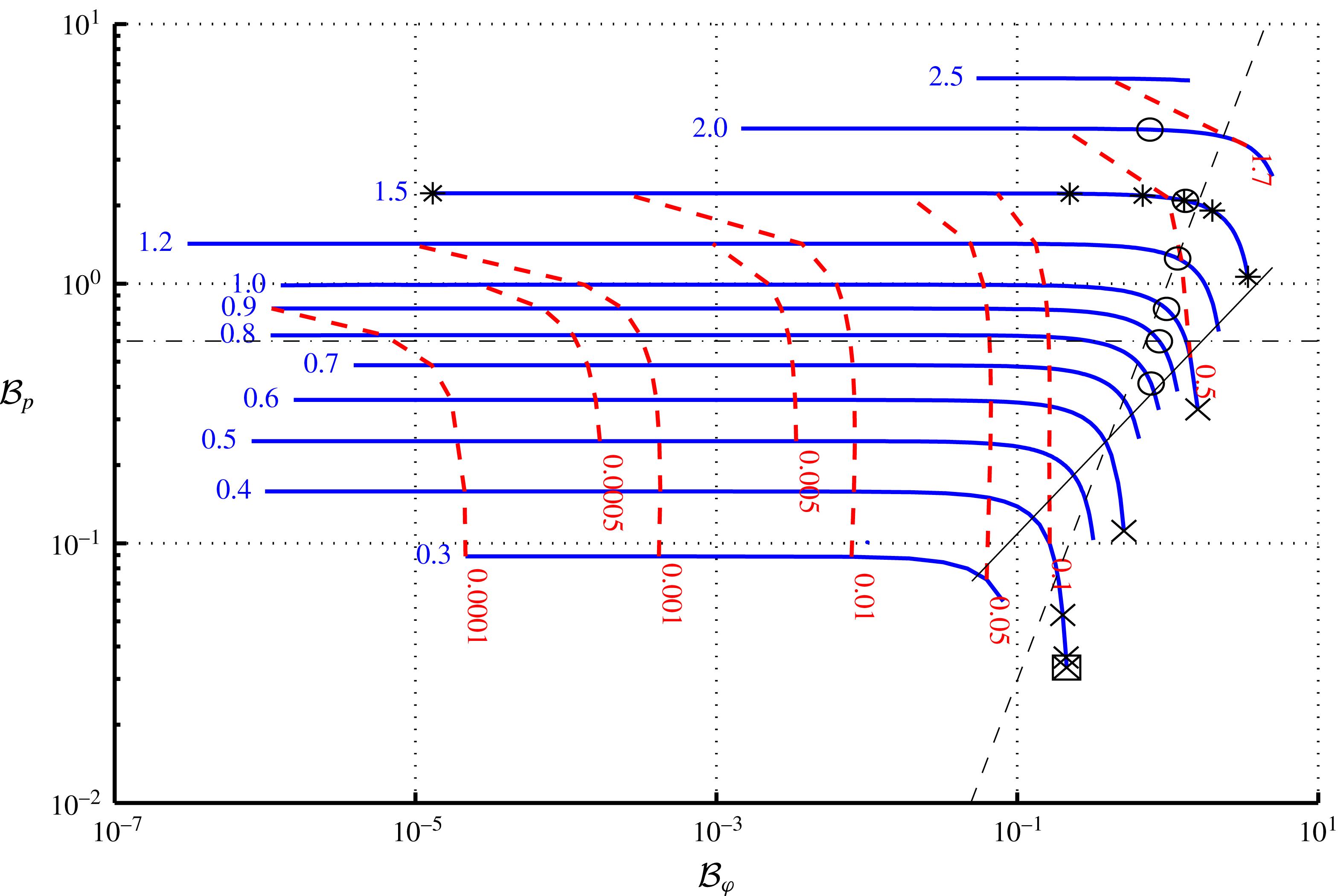
Reference Boudesocque-Dubois, Gauthier and Clarisse2008, Reference Boudesocque-Dubois, Lombard, Gauthier and Clarisse2013): see figure 3. The resulting set of solutions corresponds to a region of the
 $({\mathcal{B}}_{\unicode[STIX]{x1D711}},{\mathcal{B}}_{p})$
parameter space spanning seven decades in
 ${\mathcal{B}}_{\unicode[STIX]{x1D711}}$
and more than two decades in
 ${\mathcal{B}}_{p}$
. For each value of
 $\unicode[STIX]{x1D709}_{sf}$
, the lowest achievable value of
 ${\mathcal{B}}_{\unicode[STIX]{x1D711}}$
is determined by the fulfillment of criterion (C1). Largest achievable values of
 ${\mathcal{B}}_{\unicode[STIX]{x1D711}}$
are constrained by:
(i) For the smallest values of
$\unicode[STIX]{x1D709}_{sf}$
: limitations on the highest solution stiffnesses and smallest boundary fluid densities
$G(0)$
that can be handled by the numerical method.(ii) For the largest values of
$\unicode[STIX]{x1D709}_{sf}$
: fulfillment of criterion (C2) since increasing values of the boundary pressure
${\mathcal{B}}_{p}$
and heat flux
${\mathcal{B}}_{\unicode[STIX]{x1D711}}$
induce larger extents of the bounding double wave front structure.


Chart
 $({\mathcal{B}}_{\unicode[STIX]{x1D711}},{\mathcal{B}}_{p})$
of invariant-density self-similar ablative solutions in the non-isothermal bounding shock-wave approximation for
 $(\unicode[STIX]{x1D6FE}=5/3,\unicode[STIX]{x1D707}=2,\unicode[STIX]{x1D708}=13/2)$
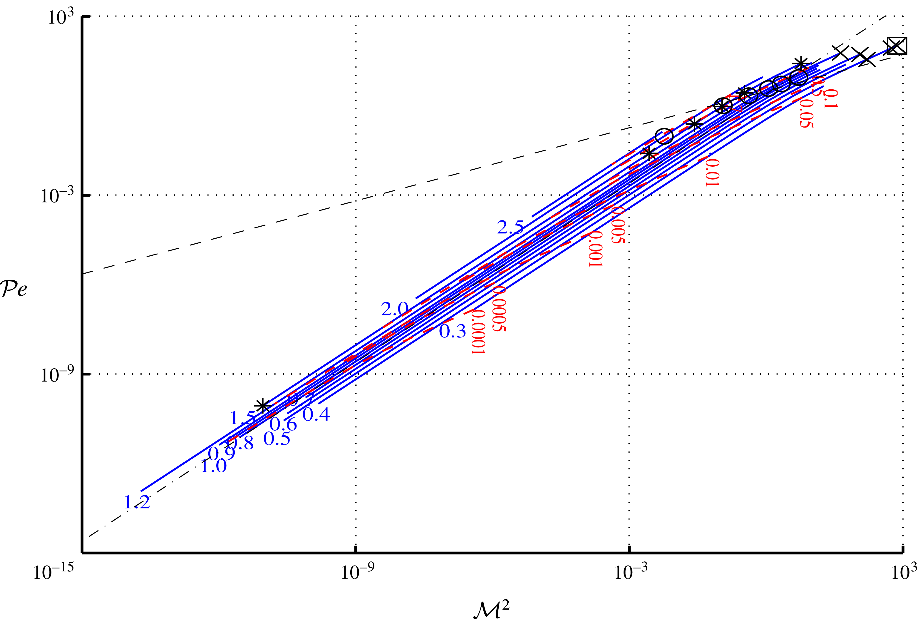
. This chart represents 631 numerical solutions to the nonlinear eigenvalue problem (3.5), (3.7), (3.8), that satisfy criteria (C1) and (C2). Sets of solutions with constant shock front reduced abscissa
 $\unicode[STIX]{x1D709}_{sf}$
(
 $-\!\!-$
, blue) are labelled with the corresponding values of
 $\unicode[STIX]{x1D709}_{sf}$
. Some of the sets of solutions with constant
 $\unicode[STIX]{x1D709}_{f}$
, the a priori estimate of the conduction-flux minimum location, are also plotted (
 $-\,-\,-$
, red) and labelled with their values of
 $\unicode[STIX]{x1D709}_{f}$
. Several particular flows are distinguished: a solution sample such that
 $\unicode[STIX]{x1D709}_{sf}=1.5$
(
 $\ast$
), another sample with
 $\unicode[STIX]{x1D709}_{f}/\unicode[STIX]{x1D709}_{sf}=0.4$
(○), flows with isentropic Chapman–Jouguet points (
 $\times$
) and a flow extrapolated from an ICF pellet implosion (IPI) simulation – IPI-like flow (▫). Flows dominantly driven by hydrodynamics (heat conduction) are located above (respectively, below) the line
 $c_{c}/d_{c}=1$
(
 $-\,\boldsymbol{\cdot }\,-$
), according to the flow-scale-based estimate (3.13), or, according to the more refined estimate (3.14), to the left (respectively, right) of the line
 $v_{pw}(t)/v_{tw}(t)=1$
(
 $-\,-\,-$
). In addition, the set of solutions with vanishing external boundary velocity, i.e. such that
 $V(0)\approx 0$
, is indicated (
 $-\!\!-$
). This set which is made of a one-parameter family of solutions, corresponds to the tamped ablation flows studied in Sanz et al. (Reference Sanz, Piriz and Tomasel1992). Solutions with positive (negative) boundary velocity lie to the left (respectively, right) of this set.

The penetration of the leading shock wave into the fluid – measured by the shock front velocity
 $D$
, equivalently
 $\unicode[STIX]{x1D709}_{sf}$
– is seen (figure 3) to increase mainly with the boundary pressure
 ${\mathcal{B}}_{p}$
(the boundary heat flux
 ${\mathcal{B}}_{\unicode[STIX]{x1D711}}$
) for sufficiently low (respectively, high) values of
 ${\mathcal{B}}_{\unicode[STIX]{x1D711}}$
relatively to
 ${\mathcal{B}}_{p}$
. In particular, as expected when heat diffusion becomes negligible, the limiting behaviour
 $\unicode[STIX]{x1D709}_{sf}\sim \text{const}\,{\mathcal{B}}_{p}^{1/2}$
is observed for
 ${\mathcal{B}}_{\unicode[STIX]{x1D711}}\ll {\mathcal{B}}_{p}$
. The a priori estimate of the conduction-flux minimum reduced abscissa,
 $\unicode[STIX]{x1D709}_{f}$
, which is indicative of the heat wave penetration into the fluid, appears to essentially increase with the boundary heat flux
 ${\mathcal{B}}_{\unicode[STIX]{x1D711}}$
provided that the boundary pressure
 ${\mathcal{B}}_{p}$
is no too high by comparison with
 ${\mathcal{B}}_{\unicode[STIX]{x1D711}}$
(figure 3). As
 ${\mathcal{B}}_{p}$
gets larger this dependency of
 $\unicode[STIX]{x1D709}_{f}$
on
 ${\mathcal{B}}_{\unicode[STIX]{x1D711}}$
becomes weaker, indicating that the corresponding flows are increasingly dominated by hydrodynamics rather than by heat diffusion. Flows that are dominantly driven by their external boundary heat flux are characterized by sensitivities of both the shock-wave and heat-wave penetration,
 $\unicode[STIX]{x1D709}_{sf}$
and
 $\unicode[STIX]{x1D709}_{f}$
, that are the strongest with respect to
 ${\mathcal{B}}_{\unicode[STIX]{x1D711}}$
and the weakest with respect to
 ${\mathcal{B}}_{p}$
. Such flows, found for values of
 ${\mathcal{B}}_{\unicode[STIX]{x1D711}}$
that are sufficiently high relative to
 ${\mathcal{B}}_{p}$
(figure 3), cannot be identified on the sole basis of large values of the Clausius number
 $\mathit{Cl}=\unicode[STIX]{x1D70C}_{I}\,v_{\star }^{3}/\unicode[STIX]{x1D711}_{\unicode[STIX]{x1D6E4}}=1/{\mathcal{B}}_{\unicode[STIX]{x1D711}}$
(Boudesocque-Dubois et al.
Reference Boudesocque-Dubois, Gauthier and Clarisse2008) which only depends on
 ${\mathcal{B}}_{\unicode[STIX]{x1D711}}$
.
Some particular flows are highlighted on the chart of figure 3 as they will be used in the subsequent analysis for illustrative purposes, namely:
(i) A sample of solutions such that
$\unicode[STIX]{x1D709}_{sf}=1.5$
.(ii) Another sample with
$\unicode[STIX]{x1D709}_{f}/\unicode[STIX]{x1D709}_{sf}=0.4$
.(iii) Solutions presenting isentropic Chapman–Jouguet points (cf. appendix B of the supplementary material).
(iv) A solution extrapolated from a simulation with a multi-physics hydrodynamics code, with grey radiative diffusion, of the early irradiation phase of an ICF-pellet implosion (IPI) – IPI-like flow.


The subset of solutions with vanishing external boundary velocity (i.e. for which
 $V(0)\approx 0$
), which corresponds to the approximate equation
 ${\mathcal{B}}_{p}=0.437451\,{\mathcal{B}}_{\unicode[STIX]{x1D711}}^{0.604794}$
, is also indicated (figure 3).


3.2 Chart
$({\mathcal{M}}^{2},{\mathcal{P}}\mathit{e})$
for
$(\unicode[STIX]{x1D6FE}=5/3,\unicode[STIX]{x1D707}=2,\unicode[STIX]{x1D708}=13/2)$


The classification in the plane
 $({\mathcal{M}}^{2},{\mathcal{P}}\mathit{e})$
of the solutions computed for (
 $\unicode[STIX]{x1D6FE}=5/3$
,
 $\unicode[STIX]{x1D707}=2$
,
 $\unicode[STIX]{x1D708}=13/2$
) is readily obtained from the chart
 $({\mathcal{B}}_{\unicode[STIX]{x1D711}},{\mathcal{B}}_{p})$
by applying the expressions of table 2: see figure 4. In the plane
 $({\mathcal{M}}^{2},{\mathcal{P}}\mathit{e})$
, lines of constant
 ${\mathcal{B}}_{p}$
– i.e. of equations
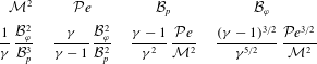
 $$\begin{eqnarray}{\mathcal{P}}\mathit{e}=(\unicode[STIX]{x1D6FE}^{2}/(\unicode[STIX]{x1D6FE}-1))\,{\mathcal{B}}_{p}\,{\mathcal{M}}^{2},\end{eqnarray}$$
as deduced from the relation
 ${\mathcal{B}}_{p}({\mathcal{M}},{\mathcal{P}}\mathit{e})$
given in table 2 – appear as straight lines of unit slope in the
 $\log$
–
 $\log$
representation of figure 4. Solutions are thus distributed among these lines according to their value of the parameter
 ${\mathcal{B}}_{p}$
and along each of these lines according to their value of
 ${\mathcal{M}}^{2}$
, or, equivalently, of
 ${\mathcal{P}}\mathit{e}$
. Lines of constant
 $\unicode[STIX]{x1D709}_{sf}$
follow lines of constant
 ${\mathcal{B}}_{p}$
for sufficiently small values of the Péclet scale
 ${\mathcal{P}}\mathit{e}$
: more precisely, the limiting behaviour
 $\unicode[STIX]{x1D709}_{sf}\sim \text{const}\,{\mathcal{B}}_{p}^{1/2}$
is found to be verified for
 ${\mathcal{P}}\mathit{e}\;(\propto {\mathcal{B}}_{\unicode[STIX]{x1D711}}^{2}/{\mathcal{B}}_{p}^{2})\;\ll 1$
. The whole set of solutions lies within a band about the line
 ${\mathcal{P}}\mathit{e}={\mathcal{M}}^{2}$
in the
 $\log$
–
 $\log$
representation of figure 4, with values of
 ${\mathcal{M}}^{2}$
and
 ${\mathcal{P}}\mathit{e}$
ranging from approximately
 $10^{-14}$
up to nearly
 $10^{3}$
. In terms of coefficients of (2.21), such extensive ranges represent huge variations in compressibility and diffusivity for the flows ruled by these equations.
Chart
 $({\mathcal{M}}^{2},{\mathcal{P}}\mathit{e})$
of invariant-density self-similar ablative solutions in the non-isothermal bounding shock-wave approximation for
 $(\unicode[STIX]{x1D6FE}=5/3,\unicode[STIX]{x1D707}=2,\unicode[STIX]{x1D708}=13/2)$
. Conventions are identical to those of figure 3 apart from the set of solutions with vanishing external boundary velocities which is not shown here. In this chart, flows dominantly driven by hydrodynamics (heat conduction) are located to the upper left (respectively, lower right) of the line
 $c_{c}/d_{c}=1$
(
 $-\,\boldsymbol{\cdot }\,-$
), according to the flow-scale-based estimate (3.13), or, according to the more appropriate estimate (3.14), below (respectively, above) the line
 $v_{pw}(t)/v_{tw}(t)=1$
(
 $-\,-\,-$
).

Ordering solutions into iso-
 ${\mathcal{B}}_{p}$
sets amounts in fact to classifying solutions according to their values of the reference velocity ratio
 $c_{c}/d_{c}$
, where
 $d_{c}=\sqrt{\unicode[STIX]{x1D705}_{0}/R\,\unicode[STIX]{x1D70C}_{I}\,t_{c}}$
is a reference diffusion velocity, since (cf. (2.19) and tables 1
a, 2)
 $$\begin{eqnarray}\big(c_{c}/d_{c}\big)^{2}=\unicode[STIX]{x1D6FE}\,R\,\unicode[STIX]{x1D705}_{0}^{-1}\,p_{\unicode[STIX]{x1D6E4}}\,t_{c}=\unicode[STIX]{x1D6FE}\,{\mathcal{B}}_{p}\propto \frac{{\mathcal{P}}\mathit{e}}{{\mathcal{M}}^{2}}.\end{eqnarray}$$
Taking
 $c_{c}$
and
 $d_{c}$
as being velocity scales of, respectively, the main pressure and thermal waves penetrating the fluid, this ratio may be held as an indicator of the relative importance of hydrodynamics over heat conduction as the main motion-driving mechanism (Zel’dovich & Raizer Reference Zel’dovich and Raizer1967, chapter 10, § 8). However, being built with the sole flow variable scales (table 1
b.ii), without relying on more specific flow properties, this ratio can only be considered to be a crude estimate of the weight of hydrodynamics over conduction effects as evidenced by the independence of (3.13) with respect to
 ${\mathcal{B}}_{\unicode[STIX]{x1D711}}$
. A more refined estimate is obtained upon following Zel’dovich & Raizer (Reference Zel’dovich and Raizer1967), i.e. by taking into account the self-similar nature and the double wave structure of the flows, under the form of the following relation between approximate velocities for pressure (
 $pw$
) and thermal waves (
 $tw$
),
 $$\begin{eqnarray}\frac{v_{pw}(t)}{v_{tw}(t)}\propto \frac{{\mathcal{B}}_{p}^{1/2}}{{\mathcal{B}}_{\unicode[STIX]{x1D711}}^{\unicode[STIX]{x1D708}/(\unicode[STIX]{x1D708}+2)}}.\end{eqnarray}$$
Indeed, heat-flux-dominated flows characterized by the strongest sensitivities to
 ${\mathcal{B}}_{\unicode[STIX]{x1D711}}$
of the shock-wave and heat-wave penetrations (cf. § 3.1) are observed to lie in the region
 $v_{pw}(t)/v_{tw}(t)<1$
of figures 3 and 4.
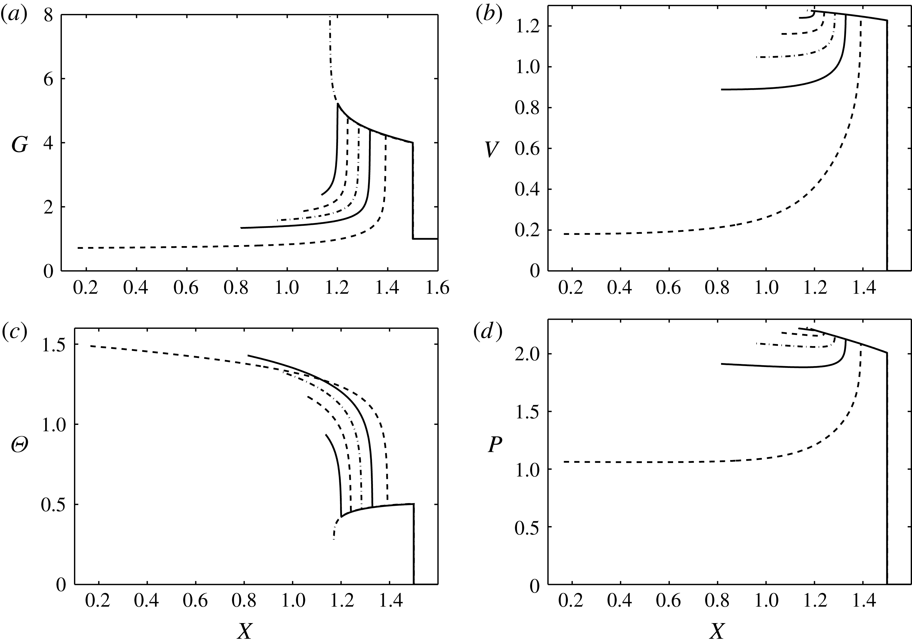
Reduced function profiles in the reduced coordinate
 $X$
of solutions obtained with the
 $({\mathcal{B}}_{p},{\mathcal{B}}_{\unicode[STIX]{x1D711}})$
-formulation – solution sample
 $\unicode[STIX]{x1D709}_{sf}=1.5$
(symbols
 $\ast$
in figure 3). Flow reduced (a) density
 $G$
, (b) velocity
 $V$
, (c) temperature
 $\unicode[STIX]{x1D6E9}$
, and (d) pressure
 $P$
. Shock-wave fronts are represented by vertical lines. In this set of flows, the profiles of smallest extent in
 $X$
, clearly outstanding, are typical of flows with vanishing conduction regions.

4 Hydrodynamic analysis
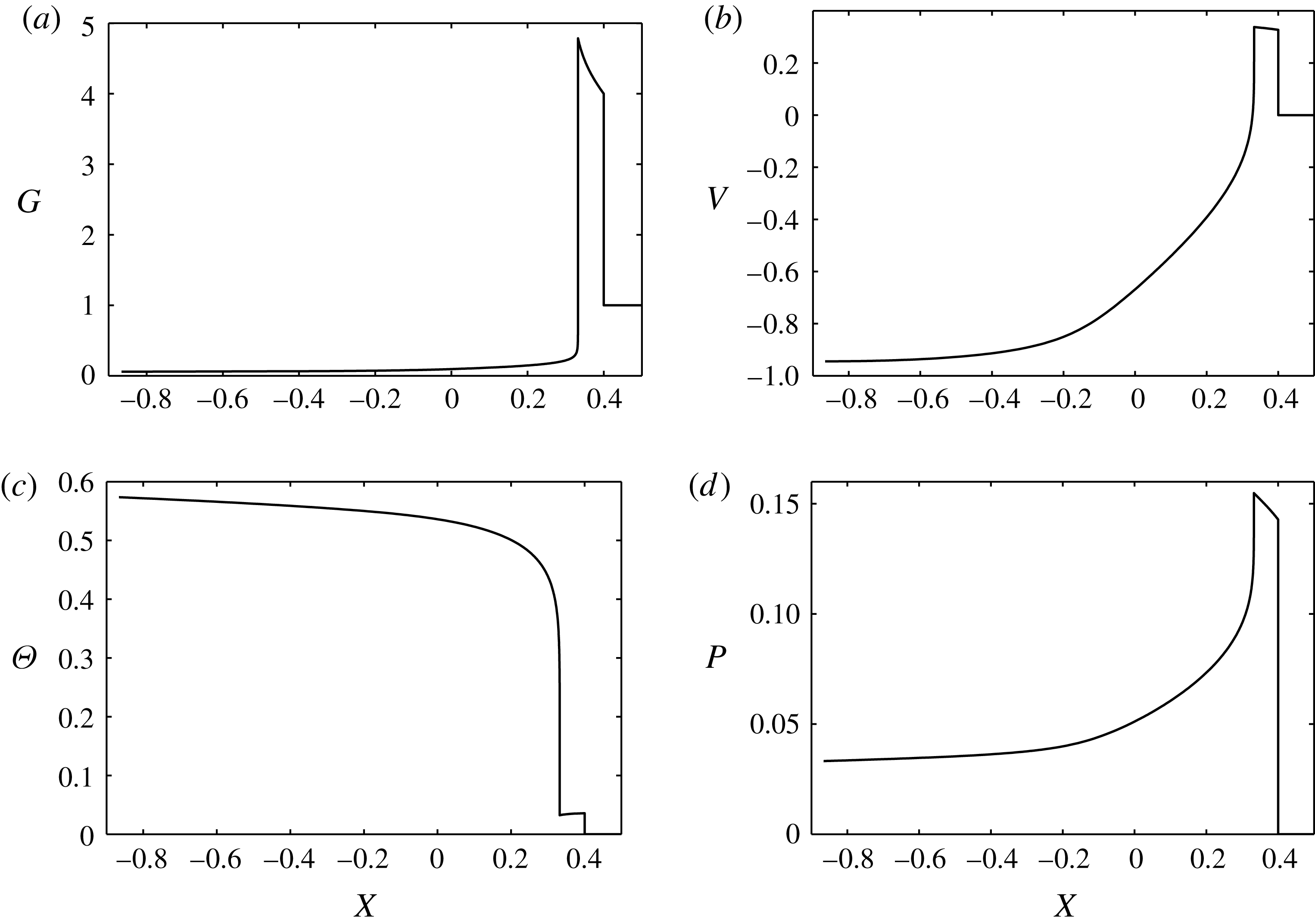
The self-similar solutions considered in the present study display the characteristic structure of an ablative heat wave penetrating a fluid initially cold and at rest under the action of an external heat source: see figure 1 (cf. also Pakula & Sigel Reference Pakula and Sigel1985; Sanz et al. Reference Sanz, Piriz and Tomasel1992). Four regions that are typical of such flows may be more or less easily identified depending on the flow stiffness or contrast, namely (see figures 1, 5–7, for increasing abscissas):
(i) The conduction region, adjacent to the fluid external boundary and characterized by the inward propagation of heat concurrently to the expansion of the heated fluid. With the adopted conventions, this region is the domain extending from the flow external surface with decreasing temperature (figures 5–7 c) and increasing fluid density (figures 5–7 a).
(ii) The ablation layer, associated with the subsonic thermal-wave front and identified by the steepest negative gradients in temperature (figures 5–7 c) and positive gradients in density (figures 5–7 a).
(iii) The compressed fluid region, extending upstream to the ablation layer up to the leading shock-wave front and corresponding to the highest fluid densities (figures 5–7 a) and lowest temperatures (figures 5–7 c).
(iv) The undisturbed fluid region, which corresponds to the fluid in its initial state of rest upstream to the leading shock front.
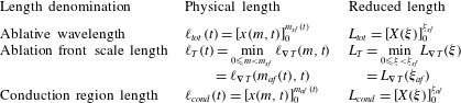
These regions are formally defined in terms of their boundaries (table 3) upon assimilating the ablation layer to a front, of finite thickness, with a definite location, chosen here to be the locus of the minimum gradient length in temperature.
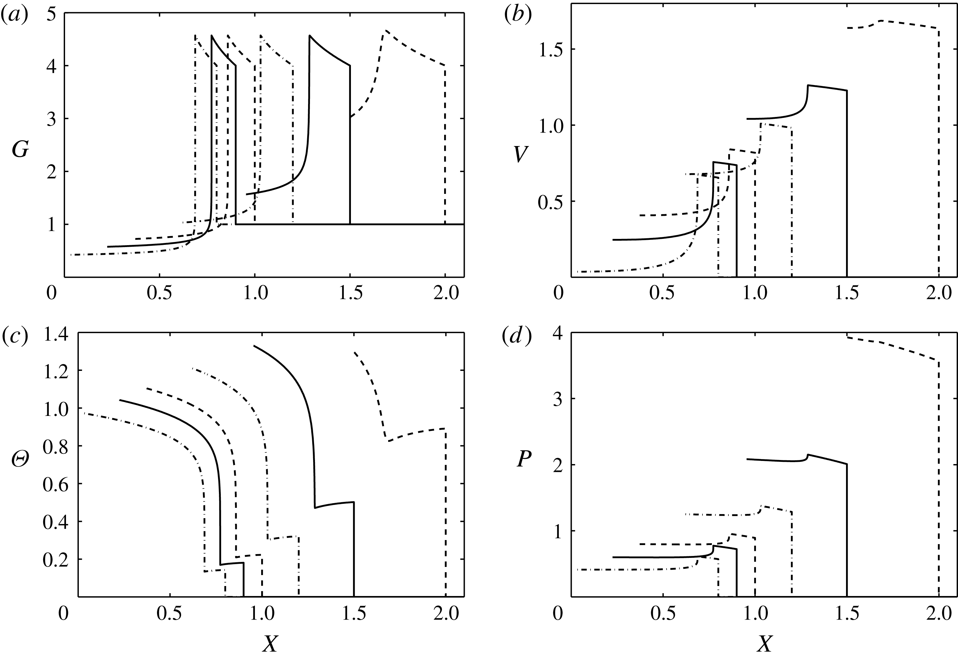
Reduced function profiles in the reduced coordinate
 $X$
of solutions obtained with the
 $({\mathcal{B}}_{p},{\mathcal{B}}_{\unicode[STIX]{x1D711}})$
-formulation – solution sample
 $\unicode[STIX]{x1D709}_{f}/\unicode[STIX]{x1D709}_{sf}=0.4$
(symbols
 $\circ$
in figure 3). Conventions identical to those of figure 5.


4.1 Flow properties
Flow properties of the self-similar ablative waves of figures 3 and 4 are investigated in a systematic manner by means of a quantitative analysis of the flow conduction region and ablation front characteristic lengths,
 $\ell _{cond}$
and
 $\ell _{T}$
, and of Mach, Péclet, stratification and Froude numbers (see appendix B of the supplementary material). The characteristic lengths
 $\ell _{cond}$
and
 $\ell _{T}$
are retained due to their influential role in the dynamics of ablation front perturbations (e.g. see Goncharov et al.
Reference Goncharov, Skupsky, Boehly, Knauer, Mckenty, Smalyuk, Town, Gotchev, Betti and Meyerhofer2000; Clarisse et al.
Reference Clarisse, Gauthier, Dastugue, Vallet and Schneider2016). Definitions of Péclet, stratification and Froude numbers (B 3)–(B 6) are purposely chosen to be given in terms of local gradient lengths so as to faithfully render the flow local properties. The corresponding analysis is conducted with the help of the two solution classifications associated with the charts
 $({\mathcal{B}}_{\unicode[STIX]{x1D711}},{\mathcal{B}}_{p})$
and
 $({\mathcal{M}}^{2},{\mathcal{P}}\mathit{e})$
of figures 3 and 4.
Four main hydrodynamic regimes stand out from the set of flows represented in these charts, namely (cf. also table 4):
(I) Two compressible flow regimes:
(i) Ablative waves with fast expansion (
$\text{fe}$
) of their conduction region. These flows are defined by supersonic velocities, relatively to the ablation front, of the heated fluid or, equivalently, by the existence of an isentropic Chapman–Jouguet point. The corresponding self-similar solutions are identified by large values of their Péclet scale
${\mathcal{P}}\mathit{e}$
– equivalently sufficiently small value of the external boundary pressure with respect to the external radiative heat flux – and lie in the region of heat-conduction-dominated flows according to the criterion
$v_{pw}(t)/v_{tw}(t)<1$
with (3.14): see figures 3 and 4. This regime comprises flows that are representative of ICF pellet implosions.(ii) Ablative waves with fast ablation (
$\text{fa}$
) characterized by a sufficiently high ablation velocity for compressible effects within the ablation layer and throughout the flow to be non-negligible. These waves correspond to solutions obtained for the largest values of the external radiative heat flux and are at the limit of validity of the non-isothermal shock-wave approximation as formalized by criterion (C2) of § 3.1.
(II) Acceleration-dominated (
$\text{ad}$
) ablative waves identified by Froude numbers below one. Relevant flows are driven by sufficiently high values of their external boundary pressure with respect to the external radiative heat flux (cf. table 4) and are dominated by hydrodynamic effects – i.e. the criterion
$v_{pw}(t)/v_{tw}(t)>1$
with (3.14) is verified. Such flows may present strongly accelerated ablation fronts, with relevant Froude numbers below
$10^{-1}$
, and are thus prone to ablative Rayleigh–Taylor instabilities (e.g. cf. Betti et al.
Reference Betti, Goncharov, Mccrory, Sorotokin and Verdon1996).(III) Ablative waves with convection-dominated ablation (
$\text{cda}$
), i.e. of Froude numbers at the ablation front larger than one. This regime which is relevant to the early ablation of an ICF target (e.g. see Velikovich et al.
Reference Velikovich, Dahlburg, Gardner and Taylor1998; Goncharov et al.
Reference Goncharov, Skupsky, Boehly, Knauer, Mckenty, Smalyuk, Town, Gotchev, Betti and Meyerhofer2000), includes flows that are typical of some ICF pellet implosions (IPI-like flow).


Definitions of geometric and characteristic lengths of the flow regions relevant to invariant-density self-similar ablative solutions in the non-isothermal bounding shock-wave approximation. Locations of the shock/ablation front (
 $sf/af$
) are identified by
 $x_{sf/af}$
in the Cartesian coordinate
 $x$
, by
 $\unicode[STIX]{x1D709}_{sf/af}$
in the reduced coordinate
 $\unicode[STIX]{x1D709}$
, and by
 $m_{sf/af}(t)=m_{\star }\,\unicode[STIX]{x1D709}_{sf/af}\,(t/t_{\star })^{\unicode[STIX]{x1D6FC}}$
in the Lagrangian coordinate
 $m$
. Additional conventions are given in table 7.

Identified hydrodynamic regimes, determining criteria (

 $({\mathcal{B}}_{\unicode[STIX]{x1D711}},{\mathcal{B}}_{p})$
or
 $({\mathcal{M}}^{2},{\mathcal{P}}\mathit{e})$
.

A further characterization of the present ablative waves results from the examination, in terms of hydrodynamic characteristic numbers, of the three main flow regions (see § B.2 of the supplementary material available at https://doi.org/10.1017/jfm.2018.343). Convective effects in the conduction region are consistently observed to be moderately outweighed by heat diffusion while compressibility effects, namely flow regime and stratification, can be at their highest levels: supersonic velocities for the regime
 $\text{fe}$
, large to infinite stratifications for some subsonic flows. The effects of acceleration are strongly varying across this region, ranging from being overwhelming to possibly being negligible in front of convection, thus testifying of the inhomogeneity of the corresponding expansion flows. The ablation layer, location of the flow steepest gradients, is markedly inhomogeneous in terms of heat diffusion, acceleration and convection effects. Non-negligible compressible effects, despite the intrinsic subsonic character of ablative waves, are expected for the fastest ablation cases. The compressed fluid region, more homogeneous in space than the rest of the flow, is characterized by comparable effects of pressure and acceleration dominating convective effects which themselves prevail over heat diffusion.
In view of the inhomogeneity and compressibility displayed by some of these ablative waves, the question of the relevance of a low Mach number approximation naturally arises. In ICF, such an approximation – or ‘isobaric model’ (Kull & Anisimov Reference Kull and Anisimov1986) as it is known in this field – has been used in many instances for modelling laser ablation flows and studying their hydrodynamic stability. In the present cases, compressibility restricts the validity of a low Mach number approximation to a limited neighbourhood of the ablation front, either because of too large fluid velocities in the fast ablation (
 $\text{fa}$
) or fast expansion (
 $\text{fe}$
) regimes, either because of excessive flow stratifications in all the other cases (§ B.3 of the supplementary material). In particular, a low Mach number description thus turns out to be inadequate at modelling ablative flows with fast expansions that are typical (e.g. Saillard et al.
Reference Saillard, Arnault and Silvert2010) of ICF-pellet implosions driven by hohlraum-generated X-ray irradiation.
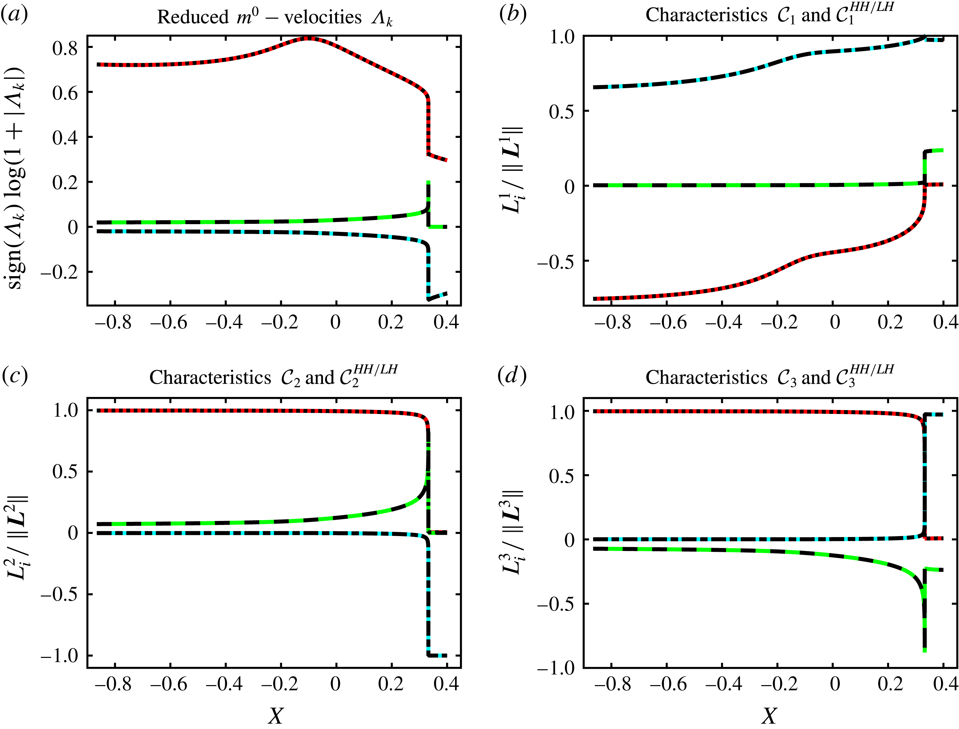
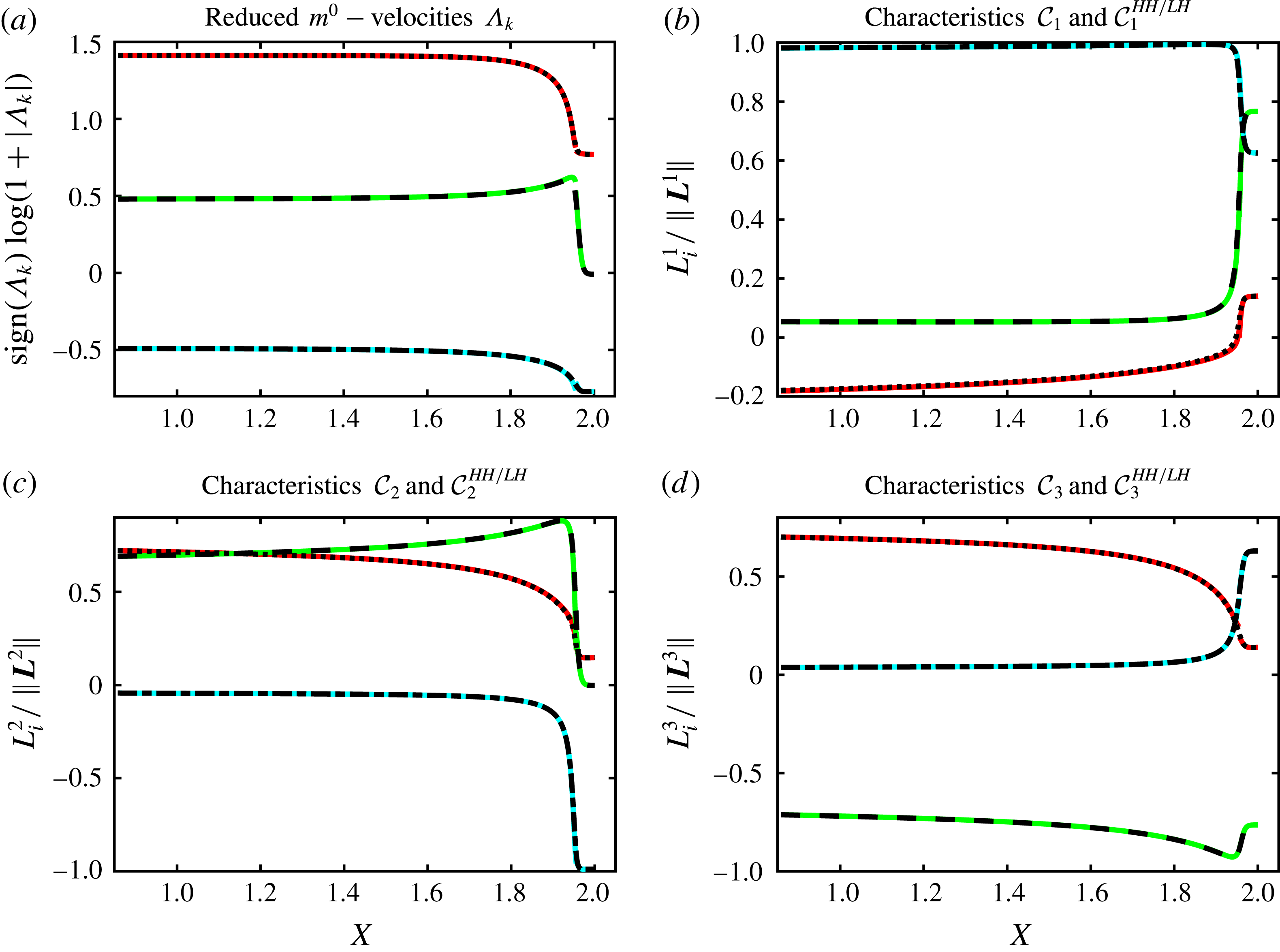
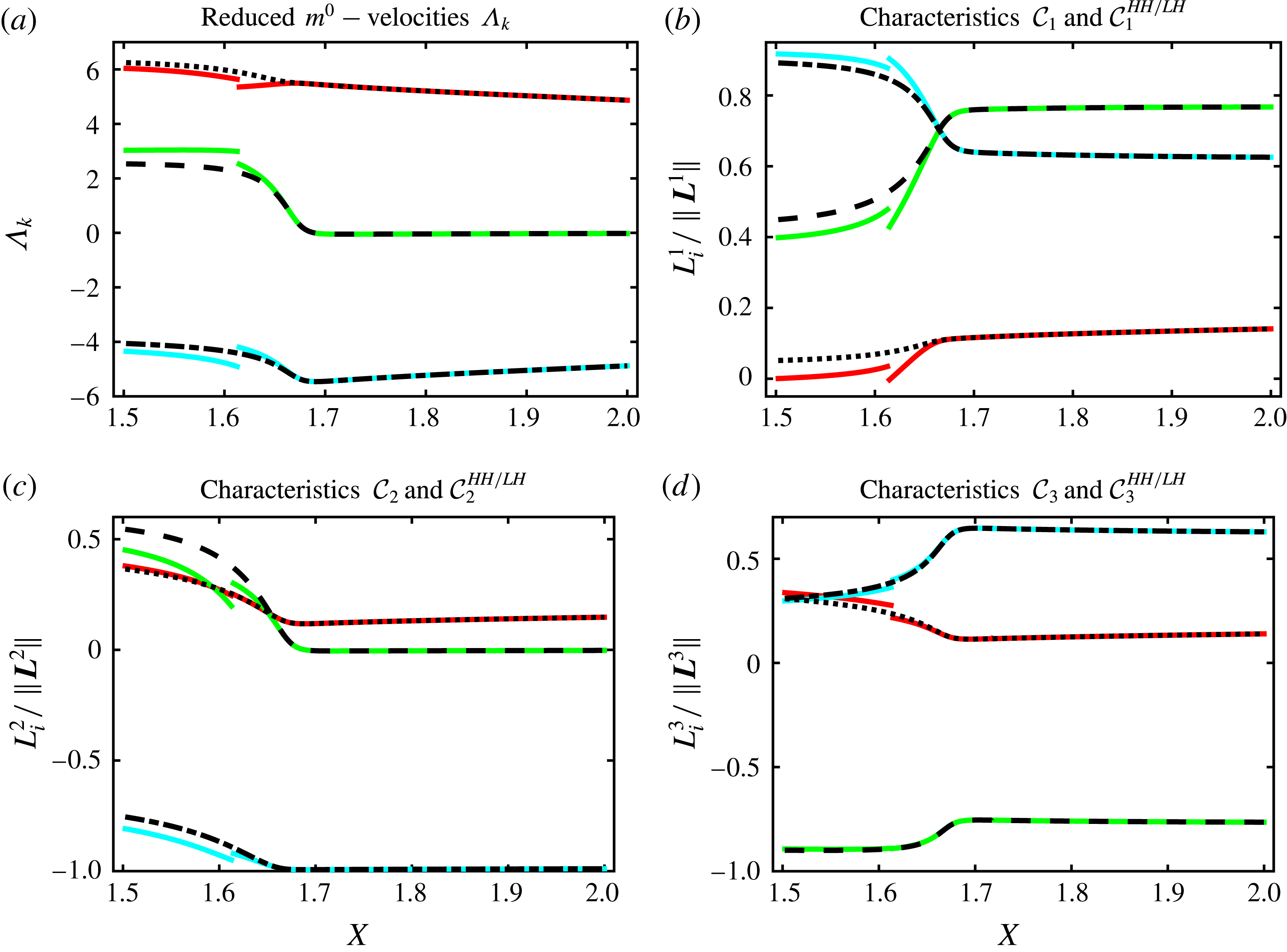
A further characterization of the compressibility properties of the present examples of radiative ablation waves is provided by a study of linear-wave propagation in such flows.
4.2 Linear waves
Analysis of linear waves in ablation flows has been previously performed in the context of ICF with the purpose of (i) obtaining practical models of steady laser, or radiative, ablation and (ii) modelling hydrodynamic instabilities of laser ablation. However, simplifying mean flow assumptions that are constitutive of these models may hinder an adequate description of linear-wave properties in actual ablation flows. In effect, the assumption of a quasi-isothermal expansion of the heated fluid in the standard model of steady radiative ablation (Nozaki & Nishihara Reference Nozaki and Nishihara1980; Nishihara Reference Nishihara1982; Atzeni & Meyer-ter-Vehn Reference Atzeni and Meyer-ter-Vehn2004; Saillard et al. Reference Saillard, Arnault and Silvert2010) reduces wave propagation in this part of the flow to that of isothermal acoustics. Moreover, as exemplified by the self-similar ablative waves of § 3, this assumption is not necessarily met in ablation flows driven by radiation conduction. Models of ablation flow hydrodynamic instabilities developed for steady laser ablation, whether accelerated or inertial, ignore the unsteady rarefaction-wave part of the flow (cf. Bychkov, Modestov & Law Reference Bychkov, Modestov and Law2015) which, in the case of radiative ablation, is an integral part of the ablative wave. In addition, linear-wave properties that are accessible to these models are dictated by restrictive background flow assumptions – e.g. low Mach number approximation, flow uniformity or constant stratification at the scale of the perturbation characteristic length. For example, the low Mach number approximation of Kull & Anisimov (Reference Kull and Anisimov1986) leads to ‘sonic’ modes that are isochoric (e.g. Piriz, Sanz & Ibañez Reference Piriz, Sanz and Ibañez1997). The more general decomposition of flow perturbations into ‘Kovásznay modes’ (Kovásznay Reference Kovásznay1953; Chu & Kovásznay Reference Chu and Kovásznay1958) which has been used for the modelling (e.g. Ishizaki & Nishihara Reference Ishizaki and Nishihara1997; Velikovich et al. Reference Velikovich, Dahlburg, Gardner and Taylor1998) and description (Lombard et al. Reference Lombard, Gauthier, Clarisse and Boudesocque-Dubois2008) of linear perturbations in the compressed fluid region of ICF ablative flows, is hardly directly applicable to the ablation layer and the flow conduction region which are characterized by a strong temperature nonlinearity, and therefore heterogeneity, of the heat conductivity. Effects of a weak, or strong, constant heat conductivity on linear waves in inviscid homogeneous compressible fluids are well documented (Landau & Lifshitz Reference Landau and Lifshitz1987, § 77; Mihalas & Mihalas Reference Mihalas and Mihalas1984, §§ 51, 101) but the combination of strong heat conductivity and flow heterogeneity in ablative waves complicates the matter and requires a more accurate assessment of its effects on linear waves. The foregoing analysis aims at addressing, in part, this issue. We deliberately restrict our investigation to a one-dimensional setting and set aside linear-wave coupling. A more comprehensive assessment of linear-wave propagation, dissipation, refraction and coupling would be obtained from studying two-dimensional perturbations, a task that we postpone to a hydrodynamic stability analysis.
4.2.1 Linearized equations
Linear-wave propagation is hereafter investigated on the basis of the
 $(\mathit{M}^{\prime },\mathit{Fr}^{\prime },\mathit{Pe}^{\prime })$
-formulation of the equations of motion, or (2.25), (2.17), (2.18), taken in the reference frame of the fluid at rest and expressed in terms of the fluid temperature. The linearization of these equations about a particular smooth solution – or base flow, say
 $(\unicode[STIX]{x1D70C}^{0},v_{x}^{0},T^{0})$
– is carried out in terms of Eulerian perturbations (cf. Boudesocque-Dubois Reference Boudesocque-Dubois2000; Clarisse et al.
Reference Clarisse, Boudesocque-Dubois and Gauthier2008), leading to the system of equations
 $$\begin{eqnarray}\frac{\unicode[STIX]{x2202}\boldsymbol{U}_{}^{1}}{\unicode[STIX]{x2202}\bar{t}}+\unicode[STIX]{x1D63C}_{}^{0}\,\frac{\unicode[STIX]{x2202}^{2}\boldsymbol{U}_{}^{1}}{\unicode[STIX]{x2202}{m_{}^{0}}^{2}}+\unicode[STIX]{x1D63D}_{}^{0}\,\frac{\unicode[STIX]{x2202}\boldsymbol{U}_{}^{1}}{\unicode[STIX]{x2202}m_{}^{0}}+\unicode[STIX]{x1D63E}_{}^{0}\,\boldsymbol{U}_{}^{1}=\mathbf{0},\end{eqnarray}$$
where
 $m^{0}$
is the mass coordinate associated with the base flow, i.e. such that
 $\text{d}m_{}^{0}=\unicode[STIX]{x1D70C}_{}^{0}\,\text{d}\bar{x}$
,
 $\boldsymbol{U}_{}^{1}=(\unicode[STIX]{x1D70C}_{}^{1}~v_{x}^{1}~T_{}^{1})^{\top }$
is the vector of linear perturbation variables, and
 $$\begin{eqnarray}\unicode[STIX]{x1D63C}_{}^{0}=\left(\begin{array}{@{}ccc@{}}0 & 0 & 0\\ 0 & 0 & 0\\ 0 & 0 & {\displaystyle \frac{\unicode[STIX]{x1D6FE}}{\mathit{Pe }^{\prime }}}\unicode[STIX]{x1D70C}_{}^{0}\unicode[STIX]{x1D713}_{T^{\prime }}^{0}\end{array}\right),\quad \unicode[STIX]{x1D63D}_{}^{0}=\left(\begin{array}{@{}ccc@{}}0 & {\unicode[STIX]{x1D70C}_{}^{0}}^{2} & 0\\ \left({\displaystyle \frac{z_{T}^{0}}{\unicode[STIX]{x1D70C}_{}^{0}}}\right)^{2} & 0 & {\displaystyle \frac{{z_{T}^{0}}^{2}}{\unicode[STIX]{x1D70C}_{}^{0}T_{}^{0}}}\\ {\displaystyle \frac{T_{}^{0}}{\unicode[STIX]{x1D70C}_{}^{0}}}q_{\unicode[STIX]{x1D70C}}^{0} & (\unicode[STIX]{x1D6FE}-1)\unicode[STIX]{x1D70C}_{}^{0}T_{}^{0} & q_{T}^{0}\end{array}\right),\end{eqnarray}$$
 $$\begin{eqnarray}\unicode[STIX]{x1D63E}_{}^{0}=\left(\begin{array}{@{}ccc@{}}\unicode[STIX]{x1D70C}_{}^{0}{\displaystyle \frac{\unicode[STIX]{x2202}v_{x}^{0}}{\unicode[STIX]{x2202}m_{}^{0}}} & \unicode[STIX]{x1D70C}_{}^{0}{\displaystyle \frac{\unicode[STIX]{x2202}\unicode[STIX]{x1D70C}_{}^{0}}{\unicode[STIX]{x2202}m_{}^{0}}} & 0\\ -{\displaystyle \frac{1}{\unicode[STIX]{x1D6FE}{\mathit{M}^{\prime }}^{2}}}{\displaystyle \frac{T_{}^{0}}{\unicode[STIX]{x1D70C}_{}^{0}}}{\displaystyle \frac{\unicode[STIX]{x2202}\unicode[STIX]{x1D70C}_{}^{0}}{\unicode[STIX]{x2202}m_{}^{0}}} & \unicode[STIX]{x1D70C}_{}^{0}{\displaystyle \frac{\unicode[STIX]{x2202}v_{x}^{0}}{\unicode[STIX]{x2202}m_{}^{0}}} & {\displaystyle \frac{1}{\unicode[STIX]{x1D6FE}{\mathit{M}^{\prime }}^{2}}}{\displaystyle \frac{\unicode[STIX]{x2202}\unicode[STIX]{x1D70C}_{}^{0}}{\unicode[STIX]{x2202}m_{}^{0}}}\\ C_{31}^{0} & \unicode[STIX]{x1D70C}_{}^{0}{\displaystyle \frac{\unicode[STIX]{x2202}T_{}^{0}}{\unicode[STIX]{x2202}m_{}^{0}}} & C_{33}^{0}\end{array}\right),\end{eqnarray}$$
with
 $$\begin{eqnarray}C_{31}^{0}=\frac{\unicode[STIX]{x1D6FE}}{\mathit{Pe}^{\prime }}\left[\frac{\unicode[STIX]{x2202}\unicode[STIX]{x1D713}_{\unicode[STIX]{x1D70C}}^{0}}{\unicode[STIX]{x2202}m_{}^{0}}-\frac{1}{\unicode[STIX]{x1D70C}_{}^{0}}\,\frac{\unicode[STIX]{x2202}\unicode[STIX]{x1D713}_{}^{0}}{\unicode[STIX]{x2202}m_{}^{0}}\right],\quad C_{33}^{0}=(\unicode[STIX]{x1D6FE}-1)\,\unicode[STIX]{x1D70C}_{}^{0}\,\frac{\unicode[STIX]{x2202}v_{x}^{0}}{\unicode[STIX]{x2202}m_{}^{0}}+\frac{\unicode[STIX]{x1D6FE}}{\mathit{Pe}^{\prime }}\,\frac{\unicode[STIX]{x2202}\unicode[STIX]{x1D713}_{T}^{0}}{\unicode[STIX]{x2202}m_{}^{0}}.\end{eqnarray}$$
In these expressions, use has been made of the function
 $$\begin{eqnarray}\unicode[STIX]{x1D713}(\unicode[STIX]{x1D70C},T,T^{\prime })=-\bar{\unicode[STIX]{x1D705}}(\unicode[STIX]{x1D70C},T)\,T^{\prime },\end{eqnarray}$$
and of the short-hand notations
 $$\begin{eqnarray}\left.\begin{array}{@{}c@{}}\unicode[STIX]{x1D713}_{}^{0}=\unicode[STIX]{x1D711}_{x}^{0}=\unicode[STIX]{x1D713}\left(\unicode[STIX]{x1D70C}_{}^{0},T_{}^{0},\unicode[STIX]{x1D70C}_{}^{0}\unicode[STIX]{x2202}_{m_{}^{0}}T_{}^{0}\right),\quad \unicode[STIX]{x1D713}_{\unicode[STIX]{x1D70C}}^{0}=\displaystyle \frac{\unicode[STIX]{x2202}\unicode[STIX]{x1D713}}{\unicode[STIX]{x2202}\unicode[STIX]{x1D70C}}\left(\unicode[STIX]{x1D70C}_{}^{0},T_{}^{0},\unicode[STIX]{x1D70C}_{}^{0}\unicode[STIX]{x2202}_{m_{}^{0}}T_{}^{0}\right),\\ \displaystyle \unicode[STIX]{x1D713}_{T}^{0}=\displaystyle \frac{\unicode[STIX]{x2202}\unicode[STIX]{x1D713}}{\unicode[STIX]{x2202}T}\left(\unicode[STIX]{x1D70C}_{}^{0},T_{}^{0},\unicode[STIX]{x1D70C}_{}^{0}\unicode[STIX]{x2202}_{m_{}^{0}}T_{}^{0}\right),\quad \unicode[STIX]{x1D713}_{T^{\prime }}^{0}=\displaystyle \frac{\unicode[STIX]{x2202}\unicode[STIX]{x1D713}}{\unicode[STIX]{x2202}T^{\prime }}\left(\unicode[STIX]{x1D70C}_{}^{0},T_{}^{0},\unicode[STIX]{x1D70C}_{}^{0}\unicode[STIX]{x2202}_{m_{}^{0}}T_{}^{0}\right),\end{array}\right\}\end{eqnarray}$$
for the base-flow heat flux
 $\unicode[STIX]{x1D711}_{x}^{0}$
and its partial derivatives with respect to, respectively, the fluid density, temperature and temperature gradient. In addition, the notations
 $$\begin{eqnarray}z_{T}^{0}=\unicode[STIX]{x1D70C}_{}^{0}\,\sqrt{T_{}^{0}/\unicode[STIX]{x1D6FE}{\mathit{M }^{\prime }}^{2}},\end{eqnarray}$$
for the isothermal sound velocity in the coordinate
 $m_{}^{0}$
, or ‘isothermal acoustic impedance’, and
 $$\begin{eqnarray}q_{\unicode[STIX]{x1D70C}}^{0}=\frac{\unicode[STIX]{x1D6FE}}{\mathit{Pe}^{\prime }}\,\frac{\unicode[STIX]{x1D70C}_{}^{0}}{T_{}^{0}}\,\unicode[STIX]{x1D713}_{\unicode[STIX]{x1D70C}}^{0},\quad q_{T}^{0}=\frac{\unicode[STIX]{x1D6FE}}{\mathit{Pe}^{\prime }}\left[\frac{\unicode[STIX]{x2202}}{\unicode[STIX]{x2202}m_{}^{0}}(\unicode[STIX]{x1D70C}_{}^{0}\,\unicode[STIX]{x1D713}_{T^{\prime }}^{0})+\unicode[STIX]{x1D713}_{T}^{0}\right],\end{eqnarray}$$
where both
 $q_{\unicode[STIX]{x1D70C}}^{0}$
and
 $q_{T}^{0}$
are homogeneous to velocities in the coordinate
 $m_{}^{0}$
, have been introduced. The partial derivative terms
 $\unicode[STIX]{x1D713}_{\unicode[STIX]{x1D70C}}^{0}$
,
 $\unicode[STIX]{x1D713}_{T}^{0}$
in these latter quantities and in the expressions of
 $C_{31}^{0}$
and
 $C_{33}^{0}$
, stem from the conduction coefficient dependency on density and temperature, and are effective only in the case of a fluid temperature non-uniformity. Their role is critical to the foregoing analysis: through these terms, a base-flow non-uniformity not only induces source and coupling coefficients – the matrix
 $\unicode[STIX]{x1D63E}_{}^{0}$
– but also first-order derivative coefficients – the entries
 $B_{31}^{0}$
and
 $B_{33}^{0}$
of the matrix
 $\unicode[STIX]{x1D63D}_{}^{0}$
– which otherwise would not be present. In particular, the wave properties of the reduced first-order system
 $$\begin{eqnarray}\frac{\unicode[STIX]{x2202}\boldsymbol{U}_{}^{1}}{\unicode[STIX]{x2202}\bar{t}}+\unicode[STIX]{x1D63D}_{}^{0}\,\frac{\unicode[STIX]{x2202}\boldsymbol{U}_{}^{1}}{\unicode[STIX]{x2202}m_{}^{0}}=\mathbf{0},\end{eqnarray}$$
may differ significantly from those obtained for a uniform base flow, i.e. for which
 $B_{31}^{0}=B_{33}^{0}=0$
, or for the equations of isothermal gas dynamics.
4.2.2 Hyperbolic waves
The analysis, in terms of hyperbolic waves, of flows ruled by the equations of motion (2.25) requires considering the reduced system (4.9) rather than the system of isentropic or isothermal gas dynamics. The eigenvalues of the matrix
 $\unicode[STIX]{x1D63D}_{}^{0}$
, say
 $\unicode[STIX]{x1D706}_{k}$
,
 $k=1,2,3$
, may be computed, both analytically and numerically, using algebraic expressions (see appendix C of the supplementary material). These expressions are however too involved to be useful by themselves without having recourse to simplifying assumptions. Numerical evaluation of the eigenvalues
 $\unicode[STIX]{x1D706}_{k}$
is thus used in the general case, leading to the numerical formulation of the linear-wave characteristic equations
 $$\begin{eqnarray}\text{d}{w_{}^{1}}_{k}\equiv {\boldsymbol{l}^{k}}^{\top }\,\text{d}\boldsymbol{U}_{}^{1}=0,\quad \text{along }{\mathcal{C}}_{k}:\quad \frac{\text{d}m_{}^{0}}{\text{d}\bar{t}}=\unicode[STIX]{x1D706}_{k},\quad \text{for }k=1,2,3,\end{eqnarray}$$
where
 $\boldsymbol{l}^{k}$
, a left eigenvector of
 $\unicode[STIX]{x1D63D}_{}^{0}$
associated with the eigenvalue
 $\unicode[STIX]{x1D706}_{k}$
, is characterized by its numerical components
 $l_{i}^{k}$
,
 $i=1,2,3$
. A local hyperbolic wave analysis of any given computed flow consists then in studying the numerical values of
 $(\unicode[STIX]{x1D706}_{k},\boldsymbol{l}^{k})$
,
 $k=1,2,3$
, across the flow. Such an analysis is facilitated by approximate analytical expressions obtained in the two limiting regimes of heat-conduction induced velocities
 $q_{\unicode[STIX]{x1D70C}}^{0}$
,
 $q_{T}^{0}$
of (4.8) being much smaller or much larger than the acoustic impedance
 $z_{T}^{0}$
.
Low heat-propagation (LH) regime. When
 $|q_{\unicode[STIX]{x1D70C}}^{0}|\ll z_{T}^{0}$
and
 $|q_{T}^{0}|\ll z_{T}^{0}$
, expansions (C 4), (C 5) for the eigenvalues and left eigenvectors of
 $\unicode[STIX]{x1D63D}_{}^{0}$
(see appendix C of the supplementary material) result, at leading order in
 $q_{\unicode[STIX]{x1D70C}}^{0}/z_{T}^{0}$
and
 $q_{T}^{0}/z_{T}^{0}$
, in the approximate characteristic equations
 $$\begin{eqnarray}\displaystyle & \displaystyle \text{d}{w_{}^{1}}_{1}^{LH}\equiv \text{d}p_{}^{1}+\unicode[STIX]{x1D6FE}\,{\mathit{M}^{\prime }}^{2}\,\sqrt{\unicode[STIX]{x1D6FE}}\,z_{T}^{0}\,\text{d}v_{x}^{1}=0,\quad \text{along}~{\mathcal{C}}_{1}^{LH}:\quad \frac{\text{d}m_{}^{0}}{\text{d}\bar{t}}=\sqrt{\unicode[STIX]{x1D6FE}}\,z_{T}^{0},\qquad & \displaystyle\end{eqnarray}$$
 $$\begin{eqnarray}\displaystyle & \displaystyle \text{d}{w_{}^{1}}_{2}^{LH}\equiv \text{d}s_{}^{1}=0,\quad \text{along }{\mathcal{C}}_{2}^{LH}:\quad \frac{\text{d}m_{}^{0}}{\text{d}\bar{t}}=\frac{1}{\unicode[STIX]{x1D6FE}}\,(q_{T}^{0}-q_{\unicode[STIX]{x1D70C}}^{0}),\qquad & \displaystyle\end{eqnarray}$$
 $$\begin{eqnarray}\displaystyle & \displaystyle \text{d}{w_{}^{1}}_{3}^{LH}\equiv \text{d}p_{}^{1}-\unicode[STIX]{x1D6FE}\,{\mathit{M}^{\prime }}^{2}\,\sqrt{\unicode[STIX]{x1D6FE}}\,z_{T}^{0}\,\text{d}v_{x}^{1}=0,\quad \text{along}~{\mathcal{C}}_{3}^{LH}:\quad \frac{\text{d}m_{}^{0}}{\text{d}\bar{t}}=-\sqrt{\unicode[STIX]{x1D6FE}}\,z_{T}^{0},\qquad & \displaystyle\end{eqnarray}$$
 $s_{}^{1}$
is the specific entropy linear perturbation, whose expression is readily deduced after
 $\bar{s}=\bar{\text{C}_{v}}\,\ln (\bar{p}/\bar{\unicode[STIX]{x1D70C}}^{\unicode[STIX]{x1D6FE}})+\bar{s}_{0}$
. As expected, we recover with the characteristics
 ${\mathcal{C}}_{1,3}^{LH}$
the characteristics
 ${\mathcal{C}}_{\pm }^{S}$
of isentropic acoustic waves as they would come out from (4.9) with
 $q_{\unicode[STIX]{x1D70C}}^{0}=q_{T}^{0}=0$
in (4.2b
), whereas
 ${\mathcal{C}}_{2}^{LH}$
appear as a modification of the gas-dynamics entropy-wave characteristics
 ${\mathcal{C}}_{0}^{S}$
, of equation
 $$\begin{eqnarray}\text{d}s_{}^{1}=0,\quad \text{along }{\mathcal{C}}_{0}^{S}:\quad \frac{\text{d}m_{}^{0}}{\text{d}\bar{t}}=0.\end{eqnarray}$$
High heat-propagation (HH) regime. For
 $|q_{T}^{0}|\gg z_{T}^{0}$
, expansions (C 6), (C 7) for the eigenvalues and left eigenvectors of
 $\unicode[STIX]{x1D63D}_{}^{0}$
(cf. appendix C of the supplementary material) yield, at leading order in
 $z_{T}^{0}/q_{T}^{0}$
, the approximate characteristic equations
 $$\begin{eqnarray}\displaystyle & \displaystyle \text{d}{w_{}^{1}}_{1}^{HH}\equiv \frac{q_{\unicode[STIX]{x1D70C}}^{0}}{q_{T}^{0}}\,T_{}^{0}\,\text{d}\unicode[STIX]{x1D70C}_{}^{1}+\unicode[STIX]{x1D70C}_{}^{0}\,\text{d}T_{}^{1}=0,\quad \text{along }{\mathcal{C}}_{1}^{HH}:\quad \frac{\text{d}m_{}^{0}}{\text{d}\bar{t}}=q_{T}^{0}, & \displaystyle\end{eqnarray}$$
 $$\begin{eqnarray}\displaystyle & \displaystyle \text{d}{w_{}^{1}}_{2}^{HH}\equiv \left|1-\frac{q_{\unicode[STIX]{x1D70C}}^{0}}{q_{T}^{0}}\right|\,T_{}^{0}\,\text{d}\unicode[STIX]{x1D70C}_{}^{1}+\unicode[STIX]{x1D6FE}\,{\mathit{M}^{\prime }}^{2}\,z_{{\rm \small{hh}}}^{0}\,\text{d}v_{x}^{1}=0,\quad \text{along }{\mathcal{C}}_{2}^{HH}:\quad \frac{\text{d}m_{}^{0}}{\text{d}\bar{t}}=z_{{\rm \small{hh}}}^{0}, & \displaystyle \nonumber\\ \displaystyle & & \displaystyle\end{eqnarray}$$
 $$\begin{eqnarray}\displaystyle & \displaystyle \text{d}{w_{}^{1}}_{3}^{HH}\equiv \left|1-\frac{q_{\unicode[STIX]{x1D70C}}^{0}}{q_{T}^{0}}\right|\,T_{}^{0}\,\text{d}\unicode[STIX]{x1D70C}_{}^{1}-\unicode[STIX]{x1D6FE}\,{\mathit{M}^{\prime }}^{2}\,z_{{\rm \small{hh}}}^{0}\,\text{d}v_{x}^{1}=0,\quad \text{along }{\mathcal{C}}_{3}^{HH}:\quad \frac{\text{d}m_{}^{0}}{\text{d}\bar{t}}=-z_{{\rm \small{hh}}}^{0}, & \displaystyle \nonumber\\ \displaystyle & & \displaystyle\end{eqnarray}$$
 $$\begin{eqnarray}z_{{\rm \small{hh}}}^{0}=\sqrt{|1-q_{\unicode[STIX]{x1D70C}}^{0}/q_{T}^{0}|}\,z_{T}^{0}.\end{eqnarray}$$
The characteristics
 ${\mathcal{C}}_{2,3}^{HH}$
appear as alterations, through the factor
 $|1-q_{\unicode[STIX]{x1D70C}}^{0}/q_{T}^{0}|$
, of the isothermal acoustic-wave characteristics
 ${\mathcal{C}}_{\pm }^{T}$
, of equations
 $$\begin{eqnarray}\text{d}{w_{}^{1}}_{\pm }^{\text{T}}\equiv T_{}^{0}\,\text{d}\unicode[STIX]{x1D70C}_{}^{1}\pm \unicode[STIX]{x1D6FE}\,{\mathit{M}^{\prime }}^{2}\,z_{T}^{0}\,\text{d}v_{x}^{1}=0,\quad \displaystyle \text{along }{\mathcal{C}}_{\pm }^{T}:\quad \frac{\text{d}m_{}^{0}}{\text{d}\bar{t}}=\pm z_{T}^{0}.\end{eqnarray}$$
This factor, which is neutral when
 $q_{\unicode[STIX]{x1D70C}}^{0}\equiv 0$
, i.e. for heat conductivities that do not depend on the fluid density such as the Spitzer–Härm electron conductivity, induces in other cases, and in particular for radiative heat conductivities, a conductivity-modified propagation of acoustic waves. The remaining characteristic family,
 ${\mathcal{C}}_{1}^{HH}$
, is specific to the nonlinear conduction of heat in a non-uniform flow. The corresponding wave describes the supersonic propagation, at the velocity
 $q_{T}^{0}$
, of heat-flux perturbation inhomogeneities that are associated with inhomogeneities in density and temperature perturbations through the varying heat conductivity: compare the alternate formulation of (4.13a
),
 $$\begin{eqnarray}\text{d}{w_{}^{1}}_{1}^{HH}\equiv \unicode[STIX]{x1D713}_{\unicode[STIX]{x1D70C}}^{0}\,\text{d}\unicode[STIX]{x1D70C}_{}^{1}+\left[\frac{\unicode[STIX]{x2202}}{\unicode[STIX]{x2202}m_{}^{0}}(\unicode[STIX]{x1D70C}_{}^{0}\,\unicode[STIX]{x1D713}_{T^{\prime }}^{0})+\unicode[STIX]{x1D713}_{T}^{0}\right]\,\text{d}T_{}^{1}=0,\end{eqnarray}$$
with the expression of the heat-flux perturbation gradient,
 $$\begin{eqnarray}\frac{\unicode[STIX]{x2202}\unicode[STIX]{x1D711}_{x}^{1}}{\unicode[STIX]{x2202}m_{}^{0}}=\frac{\unicode[STIX]{x2202}\unicode[STIX]{x1D713}_{\unicode[STIX]{x1D70C}}^{0}}{\unicode[STIX]{x2202}m_{}^{0}}\,\unicode[STIX]{x1D70C}_{}^{1}+\frac{\unicode[STIX]{x2202}\unicode[STIX]{x1D713}_{T}^{0}}{\unicode[STIX]{x2202}m_{}^{0}}\,T_{}^{1}+\underbrace{\unicode[STIX]{x1D713}_{\unicode[STIX]{x1D70C}}^{0}\,\frac{\unicode[STIX]{x2202}\unicode[STIX]{x1D70C}_{}^{1}}{\unicode[STIX]{x2202}m_{}^{0}}+\left[\frac{\unicode[STIX]{x2202}}{\unicode[STIX]{x2202}m_{}^{0}}(\unicode[STIX]{x1D70C}_{}^{0}\,\unicode[STIX]{x1D713}_{T^{\prime }}^{0})+\unicode[STIX]{x1D713}_{T}^{0}\right]\,\frac{\unicode[STIX]{x2202}T_{}^{1}}{\unicode[STIX]{x2202}m_{}^{0}}}_{\unicode[STIX]{x2202}{w_{}^{1}}_{1}^{HH}/\unicode[STIX]{x2202}m_{}^{0}}+\unicode[STIX]{x1D70C}_{}^{1}\,\unicode[STIX]{x1D713}_{T^{\prime }}^{0}\,\frac{\unicode[STIX]{x2202}^{2}T_{}^{1}}{\unicode[STIX]{x2202}{m_{}^{0}}^{2}},\end{eqnarray}$$
as stemming from the heat-flux perturbation formulation
 $$\begin{eqnarray}\unicode[STIX]{x1D711}_{x}^{1}=\unicode[STIX]{x1D713}_{\unicode[STIX]{x1D70C}}^{0}\,\unicode[STIX]{x1D70C}_{}^{1}+\unicode[STIX]{x1D713}_{T}^{0}\,T_{}^{1}+\unicode[STIX]{x1D713}_{T^{\prime }}^{0}\,\unicode[STIX]{x1D70C}_{}^{0}\,\frac{\unicode[STIX]{x2202}T_{}^{1}}{\unicode[STIX]{x2202}m_{}^{0}}.\end{eqnarray}$$
For a heat conductivity independent of the fluid density – i.e. for
 $\unicode[STIX]{x1D713}_{\unicode[STIX]{x1D70C}}^{0}\equiv 0$
– such a wave is a propagating thermal wave. When the heat conductivity depends on the density, both density and temperature perturbations are propagated. Owing to the fact that the characteristics
 ${\mathcal{C}}_{1}^{HH}$
are ruled by the heat-conductivity dependency law, we use the term ‘heat conductivity wave’ for designating this type of wave, keeping in mind that the associated characteristic quantity,
 ${w_{}^{1}}_{1}^{HH}$
, is a heat flux.
4.2.3 Application to self-similar flows
The hyperbolic-wave analysis of the self-similar flows of § 3 is reducible to the analysis of the reduced functions for the wave speeds
 $\unicode[STIX]{x1D706}_{k}$
and the coefficients
 $l_{i}^{k}$
, namely
 $\unicode[STIX]{x1D6EC}_{k}$
and
 $L_{i}^{k}$
, of the characteristic equations (4.10): see appendix C of the supplementary material. This reduced function analysis is performed, on the basis of the
 $({\mathcal{B}}_{p},{\mathcal{B}}_{\unicode[STIX]{x1D711}})$
-formulation of the equations of motion (§ 2.2.1), on four particular solutions belonging to each of the four hydrodynamic regimes identified in § 4.1: see table 5.
Hyperbolic-wave characteristic equation parameters – fast expansion (
 $\text{fe}$
) flow: IPI-like solution of figure 3. Profiles, in the reduced coordinate
 $X$
, for the characteristics
 ${\mathcal{C}}_{k}$
(4.10) and their HH/LH regime approximations
 ${\mathcal{C}}_{k}^{HH/LH}$
given by (C 6)/(C 4) with (C 3) (cf. appendix C of the supplementary material), of: the reduced functions of the characteristic
 $m_{}^{0}$
-velocities,
 $\unicode[STIX]{x1D6EC}_{k}$
,
 $k=1,2,3$
(a); the normalized reduced coefficients,
 $L_{i}^{k}/\Vert \boldsymbol{L}^{k}\Vert$
,
 $i=1,2,3$
, for
 $k=1$
(b),
 $k=2$
(c), and
 $k=3$
(d). (a) Characteristics
 ${\mathcal{C}}_{1}$
/
 ${\mathcal{C}}_{1}^{HH/LH}$
(
 $\boldsymbol{\cdot }\!\boldsymbol{\cdot }\!\boldsymbol{\cdot }$
/
 $-\!\!-$
red),
 ${\mathcal{C}}_{2}$
/
 ${\mathcal{C}}_{2}^{HH/LH}$
(
 $-\,-\,-$
/
 $-\!\!-$
green),
 ${\mathcal{C}}_{3}$
/
 ${\mathcal{C}}_{3}^{HH/LH}$
(
 $-\,\boldsymbol{\cdot }\,-$
/
 $-\!\!-$
cyan). (b,c,d) Coefficients in
 $\text{d}\unicode[STIX]{x1D70C}_{}^{1}$
(
 $\boldsymbol{\cdot }\!\boldsymbol{\cdot }\!\boldsymbol{\cdot }$
/
 $-\!\!-$
red),
 $\text{d}v_{x}^{1}$
(
 $-\,-\,-$
/
 $-\!\!-$
green),
 $\text{d}T_{}^{1}$
(
 $-\,\boldsymbol{\cdot }\,-$
/
 $-\!\!-$
cyan) for the characteristics
 ${\mathcal{C}}_{k}$
/
 ${\mathcal{C}}_{k}^{HH/LH}$
. See figure 7 for the corresponding reduced fluid variable profiles.

Self-similar ablative-wave solutions representative of the four hydrodynamic regimes identified in § 4.1, table 4, that are selected for the quantitative hyperbolic-wave analysis. Solution governing parameters
 $({\mathcal{B}}_{\unicode[STIX]{x1D711}},{\mathcal{B}}_{p})$
in the chart of figure 3, main feature as members of the four hydrodynamic regimes and stiffnesses. Spatial profiles of the reduced fluid variables are given in figures 7 (
 $\text{fe}$
flow) and 6 (
 $\text{ad}$
/
 $\text{cda}$
flow, rightmost/leftmost curves in each graph).

Numerical results show that the eigenvalues
 $\unicode[STIX]{x1D6EC}_{k}$
are all real and distinct whence that system (4.9) is strictly hyperbolic. Correspondence of flow regions with the two heat-propagation regimes identified in the preceding section is obtained upon comparing computed values of
 $\unicode[STIX]{x1D6EC}_{k}$
,
 $L_{i}^{k}/\Vert \boldsymbol{L}^{k}\Vert$
,
 $i,k=1,2,3$
, with those obtained from the reduced forms of the approximations (C 4) or (C 6) and their resulting expressions (C 3) (appendix C of the supplementary material): cf. figures 8–11.



Hyperbolic-wave characteristic equation parameters – acceleration-dominated (
 $\text{ad}$
) flow
 $({\mathcal{B}}_{\unicode[STIX]{x1D711}},{\mathcal{B}}_{p})=(0.66,3.93)$
of the solution sample
 $\unicode[STIX]{x1D709}_{f}/\unicode[STIX]{x1D709}_{sf}=0.4$
of figure 3. Conventions identical to those of figure 8. See figure 6 (rightmost curves in each graph) for the corresponding reduced fluid variable profiles.

Hyperbolic-wave characteristic equation parameters – convection-dominated ablation (
 $\text{cda}$
) flow
 $({\mathcal{B}}_{\unicode[STIX]{x1D711}},{\mathcal{B}}_{p})=(0.78,0.41)$
of the solution sample
 $\unicode[STIX]{x1D709}_{f}/\unicode[STIX]{x1D709}_{sf}=0.4$
of figure 3. Conventions identical to those of figure 8. See figure 6 (leftmost curves in each graph) for the corresponding reduced fluid variable profiles.

LH regime. For each of the four representative flows, the compressed fluid region complies especially well with the properties of the approximate characteristics for the LH regime as deduced from (C 3), (C 4). This compliance quantitatively confirms the quasi-entropic nature of wave propagation in the compressed fluid region of ablative waves that has been assumed and used in many theoretical works on ICF ablation flow instabilities (e.g. Ishizaki & Nishihara Reference Ishizaki and Nishihara1997; Piriz et al.
Reference Piriz, Sanz and Ibañez1997; Velikovich et al.
Reference Velikovich, Dahlburg, Gardner and Taylor1998). In particular corrections to the isentropic sound velocities appear as marginal, while velocities of waves
 ${\mathcal{C}}_{2}$
show a slight downstream drift, with respect to the fluid, that is well matched by the approximation
 $(q_{T}^{0}-q_{\unicode[STIX]{x1D70C}}^{0})/\unicode[STIX]{x1D6FE}$
of (4.11b
).
HH regime. The description of the HH regime provided by (C 3), (C 6) matches the numerical data of the characteristics
 ${\mathcal{C}}_{k}$
over the conduction regions of the three flows representative of the
 $\text{fe}$
,
 $\text{fa}$
and
 $\text{cda}$
regimes (figures 8, 9 and 11). This agreement establishes that the waves
 ${\mathcal{C}}_{2,3}$
are nearly isothermal (cf. the smallness of the components in
 $\text{d}T_{}^{1}$
and, for the other components, the compliance with (4.13b,c
), in figures 8, 9 and 11
c,d) with characteristic velocities exceeding, by several per cent, the isothermal acoustic impedance
 $z_{T}^{0}$
in accordance with (4.14). Corroborating the properties of the approximate characteristic family
 ${\mathcal{C}}_{1}^{HH}$
, the characteristics
 ${\mathcal{C}}_{1}$
exhibit a supersonic propagation in the upstream direction – at Mach numbers
 $\unicode[STIX]{x1D706}_{1}/\unicode[STIX]{x1D706}_{2}\simeq q_{T}^{0}/z_{{\rm \small{hh}}}^{0}$
culminating above ten (figures 9 and 11
a) and possibly reaching 80–90 (figure 8
a) – of, essentially, density and temperature perturbations (figures 8, 9 and 11
a,b). Consequently, throughout the most part of the conduction regions of flows
 $\text{fe}$
,
 $\text{fa}$
and
 $\text{cda}$
, waves
 ${\mathcal{C}}_{1}$
are ascribable to the heat conductivity waves
 ${\mathcal{C}}_{1}^{HH}$
depicted by (4.13a
).
Transitory heat-propagation (TH) regime. The regime of comparable conduction induced velocities
 $q_{T}^{0}$
and acoustic impedances
 $z_{T}^{0}$
– or transitory heat-propagation (TH) regime – occurs in the ablation layer regions of flows
 $\text{fe}$
,
 $\text{fa}$
and
 $\text{cda}$
. This regime is in fact prevailing over the whole conduction region of flow
 $\text{ad}$
(figure 10) which resembles limited slices (of a few characteristic lengths
 $L_{T}$
in thickness) of the three other flows about their ablation front, but on a much larger spatial scale (
 $L_{tot}\approx 3\,L_{T}$
for flow
 $\text{ad}$
, cf. table 5). Despite differences between these representative flows, each family of characteristics is transformed across each of the flow ablation layers according to its own specific pattern (see table 6), with characteristic equation parameters varying monotonically across these layers and a simultaneous convergence of the three families of characteristics within a few lengths
 $L_{T}$
about the ablation front:
 $\text{d}\unicode[STIX]{x1D6EC}_{k}/\text{d}X<0$
,
 $k=1,2,3$
, for
 $|X-X_{af}|\lessapprox O(L_{T})$
. This simultaneous convergence of characteristics, which only bears on the families
 ${\mathcal{C}}_{1,2}$
in the variables
 $(\bar{x},\bar{t})$
(figure 12), enables the identification of the ablation front with the forefront edge of both a nonlinear heat-flux wave (
 ${\mathcal{C}}_{1}$
) and an acoustic-like wave (
 ${\mathcal{C}}_{2}$
).
Transformation patterns, through an ablation layer, of each of the linear-wave characteristics
 ${\mathcal{C}}_{k}$
between downstream HH (column left sides) and upstream LH (column right sides) limiting regimes, with associated variations of characteristic velocities and changes of limiting wave types.

Hyperbolic-wave characteristic
 $\bar{x}$
-velocities. Profiles, in the reduced coordinate
 $X$
, of the reduced functions for the characteristic
 $\bar{x}$
-velocities relative to the ablation front, or
 $\mathfrak{W}_{k}=\unicode[STIX]{x1D6EC}_{k}/G+V^{\prime }$
,
 $k=1,2,3$
, in each of the representative flows of the (a) fast expansion (fe), (b) fast ablation (fa), (c) acceleration-dominated (ad) and (d) convection-dominated ablation (cda) regimes of table 5. Characteristics
 ${\mathcal{C}}_{1}$
(
 $\boldsymbol{\cdot }\!\boldsymbol{\cdot }\!\boldsymbol{\cdot }$
),
 ${\mathcal{C}}_{2}$
(
 $-\,-\,-$
),
 ${\mathcal{C}}_{3}$
(
 $-\,\boldsymbol{\cdot }\,-$
). The Chapman–Jouguet point of the fast expansion flow (a), defined by
 $\mathfrak{W}_{2}=0$
, is located about
 $X=0.2$
.

4.2.4 Effects of heat diffusion
The effects of heat diffusion on the propagation of hyperbolic waves identified here above (§§ 4.2.2 and 4.2.3) are estimated on the basis of the second-order linear differential operator
 $$\begin{eqnarray}\boldsymbol{{\mathcal{L}}}(m_{\ast }^{0},\bar{t}_{\ast },\unicode[STIX]{x2202}_{m_{}^{0}}.)=-\unicode[STIX]{x1D63C}_{\ast }^{0}\,\frac{\unicode[STIX]{x2202}^{2}.}{\unicode[STIX]{x2202}{m_{}^{0}}^{2}}-\unicode[STIX]{x1D63D}_{\ast }^{0}\,\frac{\unicode[STIX]{x2202}.}{\unicode[STIX]{x2202}m_{}^{0}},\end{eqnarray}$$
which stems from considering (4.1), without its source term
 $\unicode[STIX]{x1D63E}_{}^{0}\,\boldsymbol{U}_{}^{1}$
, at some given time
 $\bar{t}_{\ast }$
and flow location
 $m_{\ast }^{0}$
, with the convention
 $\unicode[STIX]{x1D63C}_{\ast }^{0}=\unicode[STIX]{x1D63C}_{}^{0}(m_{\ast }^{0},\bar{t}_{\ast })$
,
 $\unicode[STIX]{x1D63D}_{\ast }^{0}=\unicode[STIX]{x1D63D}_{}^{0}(m_{\ast }^{0},\bar{t}_{\ast })$
. The computation of the eigenvalues, say (
 $\text{i}\,\unicode[STIX]{x1D714}_{k}$
),
 $k=1,2,3$
, of the matrices
 $$\begin{eqnarray}\boldsymbol{{\mathcal{L}}}(m_{\ast }^{0},\bar{t}_{\ast },-\text{i}\unicode[STIX]{x1D62C}),\quad \unicode[STIX]{x1D62C}\geqslant 0,\end{eqnarray}$$
gives access to the transmission factor for the propagation of local perturbations of the form
 $\boldsymbol{U}_{}^{1}(\bar{t};\unicode[STIX]{x1D62C})\,\exp (-\text{i}\unicode[STIX]{x1D62C}\,m_{}^{0})$
over the distance
 $\unicode[STIX]{x0394}m_{}^{0}$
, or
 $$\begin{eqnarray}\unicode[STIX]{x1D70F}(\unicode[STIX]{x0394}m_{}^{0})=\exp (-|\unicode[STIX]{x0394}m_{}^{0}|/d),\quad \text{with}~d=|\text{Re}(\unicode[STIX]{x1D714})|/\text{Im}(\unicode[STIX]{x1D714})\,\unicode[STIX]{x1D62C},\end{eqnarray}$$
where
 $d$
is the local damping length. For an heterogeneous and unsteady flow over the length and time scales
 $\unicode[STIX]{x0394}m_{}^{0}$
and
 $\unicode[STIX]{x0394}m_{}^{0}\,\unicode[STIX]{x1D62C}/|\unicode[STIX]{x1D714}|$
, this expression can only provide a crude estimate of actual wave transmission. For the self-similar flows of § 3, the determination of the eigenvalues of the matrices (4.20) comes down, by virtue of (C 8) (cf. appendix C of the supplementary material), to the computation of the eigenvalues
 $\text{i}\unicode[STIX]{x1D6FA}$
of the matrices
 $\boldsymbol{{\mathcal{L}}}(\unicode[STIX]{x1D709}_{\ast },-\text{i}\unicode[STIX]{x1D612})=\unicode[STIX]{x1D612}^{2}\,\text{}\underline{\unicode[STIX]{x1D63C}}_{\ast }^{0}+\text{i}\unicode[STIX]{x1D612}\,\text{}\underline{\unicode[STIX]{x1D63D}}_{\ast }^{0}$
,
 $\unicode[STIX]{x1D612}\geqslant 0$
, with the relations
 $\unicode[STIX]{x1D612}=\bar{t}_{\ast }^{\unicode[STIX]{x1D6FC}}\,\unicode[STIX]{x1D62C}$
,
 $\unicode[STIX]{x1D6FA}=\bar{t}_{\ast }\,\unicode[STIX]{x1D714}$
, and the convention that
 $\text{}\underline{\unicode[STIX]{x1D63C}}_{\ast }^{0}$
,
 $\text{}\underline{\unicode[STIX]{x1D63D}}_{\ast }^{0}$
are the values of the matrices
 $\text{}\underline{\unicode[STIX]{x1D63C}}_{}^{0}$
,
 $\text{}\underline{\unicode[STIX]{x1D63D}}_{}^{0}$
at
 $\unicode[STIX]{x1D709}=\unicode[STIX]{x1D709}_{\ast }=m_{\ast }^{0}/\bar{t}_{\ast }^{\unicode[STIX]{x1D6FC}}$
. For the four representative flows of table 5, wave phase velocities are marginally modified by heat diffusion – i.e. the relations
 $|\text{Re}(\unicode[STIX]{x1D6FA}_{k})|\approx \unicode[STIX]{x1D6EC}_{k}\,\unicode[STIX]{x1D612}$
, hold for
 $k=1,2,3$
– provided that the wavelengths are sufficiently large compared to
 $L_{T}$
– in effect for
 $0\leqslant \unicode[STIX]{x1D612}\leqslant \hat{\unicode[STIX]{x1D612}}$
with:
 $\hat{\unicode[STIX]{x1D612}}>2^{10}\,\unicode[STIX]{x1D612}_{cond}$
for flows
 $\text{fe}$
and
 $\text{cda}$
;
 $\hat{\unicode[STIX]{x1D612}}\approx 2^{3}\,\unicode[STIX]{x1D612}_{cond}$
for flow
 $\text{fa}$
;
 $\hat{\unicode[STIX]{x1D612}}\approx 2^{-3}\,\unicode[STIX]{x1D612}_{cond}$
for flow
 $\text{ad}$
, where
 $\unicode[STIX]{x1D612}_{cond}=2\unicode[STIX]{x03C0}/\unicode[STIX]{x1D709}_{af}$
is the conduction region reference wavenumber. Within these ranges, the highest damping rates,
 $\text{Im}(\unicode[STIX]{x1D6FA})$
, are found, in the conduction region, for the heat conductivity waves
 ${\mathcal{C}}_{1}$
and, in the compressed fluid region, for the entropy waves
 ${\mathcal{C}}_{2}$
. Within the conduction region of each of the flows, the damping length of the waves
 ${\mathcal{C}}_{1}$
, or
 $D_{1}=|\text{Re}(\unicode[STIX]{x1D6FA}_{1})|/\text{Im}(\unicode[STIX]{x1D6FA}_{1})\,\unicode[STIX]{x1D612}\approx \unicode[STIX]{x1D6EC}_{1}/\text{Im}(\unicode[STIX]{x1D6FA}_{1})$
, turns out to be an increasing function of
 $\unicode[STIX]{x1D709}$
, thus indicating that heat conductivity waves are less and less damped as they penetrate deeper into the expanding fluid. As a consequence, the transmission factor (4.21) for waves
 ${\mathcal{C}}_{1}$
travelling the distance
 $\unicode[STIX]{x0394}m_{}^{0}=m_{af}^{0}-m_{\ast }^{0}>0$
, evaluated at
 $m_{\ast }^{0}$
, or
 $$\begin{eqnarray}\unicode[STIX]{x1D70F}(m_{af}^{0}-m_{\ast }^{0})=\exp \left(-(m_{af}^{0}-m_{\ast }^{0})/d_{1}\right)=\exp \left(-(\unicode[STIX]{x1D709}_{af}-\unicode[STIX]{x1D709}_{\ast })/D_{1}\right),\end{eqnarray}$$
furnishes a lower bound on the actual transmission of such waves between the downstream location
 $m_{\ast }^{0}$
and the ablation front. Accordingly, transmission of heat conductivity waves across the conduction region occurs for wavelengths exceeding several times the region length, whereas waves shorter than this very length undergo severe damping (figure 13). Transmission of heat-flux perturbations of large characteristic lengths, and therefore of density and temperature inhomogeneities, from the flow external surface up to the ablation front is thus possible, even in the case of fast conduction region expansions as exemplified by flow
 $\text{fe}$
(figures 12 and 13
a).
Effects of heat diffusion on the propagation of heat conductivity waves
 ${\mathcal{C}}_{1}$
. Profiles, over the conduction regions and in the reduced coordinate
 $X$
, of the transmission factors (4.22) obtained for reduced wavenumbers
 $\unicode[STIX]{x1D612}=\unicode[STIX]{x1D612}_{cond}/2^{n}$
,
 $0\leqslant n\leqslant 6$
. Curves are indexed by their value of
 $n$
and the vertical dashed line (
 $-\,-\,-$
) indicates the ablation front location. Representative flows (cf. table 5) of the (a) fast expansion (fe), (b) fast ablation (fa), (c) acceleration-dominated (ad) and (d) convection-dominated ablation (cda) regimes.

4.2.5 Discussion
The present description of linear-wave propagation in ablative flows relies on taking into account the flow actual properties rather than those of some idealized configuration. The difference with earlier descriptions of radiative ablation is patent in the present identification of supersonic upstream propagation of heat-flux perturbations, or heat conductivity waves, across the flow conduction regions. These supersonic waves, carrying both density and temperature fluctuations, are a consequence of the flow non-uniformity and of the heat-conduction nonlinearity. By contrast, the standard assumption of a quasi-isothermal expansion region (cf. Nozaki & Nishihara Reference Nozaki and Nishihara1980; Nishihara Reference Nishihara1982; Atzeni & Meyer-ter-Vehn Reference Atzeni and Meyer-ter-Vehn2004; Saillard et al.
Reference Saillard, Arnault and Silvert2010) only allows for the propagation of density perturbations under the form of isothermal acoustic waves and the diffusion of temperature fluctuations. Within this depiction, density perturbations cannot reach, from further downstream, the Chapman–Jouguet points of fast expanding ablation flows. The situation illustrated by the present example of fast expansion flows (flow
 $\text{fe}$
of table 5) differs significantly in that heat flux, whence density, perturbations are propagated up to the ablation front and this with a limited damping provided that perturbation characteristic lengths are reasonably large (an order of magnitude larger than the conduction region size). This property which is a consequence of the radiative heat conductivity dependence on density is critical to the radiative heat transport instability (Bychenkov & Rozmus Reference Bychenkov and Rozmus2015) where density fluctuations associated with heat-flux perturbations are prone to destabilize fast radiative heat waves in inhomogeneous plasmas through the excitation of ion-acoustic waves. The present linear-wave description is able to account for such effects and thus contains proper information for the physical analysis of linear perturbation dynamics, and subsequently of instability mechanisms, in ablative flows. In particular, the decomposition of an ablative wave into regions of low and high heat-propagation regimes along with corresponding analytical approximations of characteristic waves, the identification of characteristic wave transformations across the ablation layer, are elements for a more accurate analysis of such inhomogeneous background flows with nonlinear heat conduction than that based on a classical Kovásznay mode decomposition.
5 Conclusion
We have used self-similar solutions to the Euler equations with nonlinear conduction as particular instances of unsteady radiative ablation waves with the goal of characterizing hydrodynamic properties that such flows may present. First identified by Marshak (Reference Marshak1958), these solutions which arise when submitting an initially quiescent perfectly cold and homogeneous semi-infinite slab of polytropic gas to external increasing pressures and radiation fluxes, are relevant to the description of the early ablation of a target by gas-filled hohlraum X-rays in experiments of HEDP. Our study relies on a sample of these solutions obtained under the approximation of a non-isothermal bounding shock wave and the radiative conduction model of Kramers for a fully ionized gas. The corresponding set of computed solutions is unique for its high fidelity description of the flows down to their finest scales, and its extensive exploration of external pressure and radiative flux ranges.
A quantitative hydrodynamic analysis has been conducted using two comprehensive classifications of these self-similar solutions as provided by two different dimensionless formulations of the equations of motion: one using the dimensionless boundary pressure and heat-flux reference values as driving parameters (cf. Samarskiĭ et al. Reference Samarskiĭ, Kurdyumov and Volosevich1965; Boudesocque-Dubois et al. Reference Boudesocque-Dubois, Gauthier and Clarisse2008), the other reproducing the standard Mach–Péclet form of the Euler equations with heat conduction in which the driving parameters, or ‘Mach and Péclet scales’, are chosen so as to give a priori indications of the flow compressibility and heat diffusivity. This analysis, based on local definitions of standard hydrodynamic characteristic numbers (Mach, Péclet, stratification and Froude numbers) supplemented by relative characteristic lengths of the main flow regions, allows us to identify characteristic features and hydrodynamic regimes of these regions. The highly heat diffusive, or ‘conduction’, region is characterized by a rather homogeneous, but consistently limited, dominance of heat diffusion over convection. Across this region the balance of acceleration versus convection and of acceleration versus pressure forces may vary significantly while the associated expanding flow may be entirely subsonic or partly supersonic. The ablation layer, highly heterogeneous regarding acceleration, convective and diffusive effects, is rather homogeneous with respect to its compressibility which may reach non-negligible levels while remaining in the subsonic range. Sharing similar compressibility features, the shock compressed fluid region shows comparable effects of pressure and acceleration forces prevailing over convection which itself dominates diffusion. Four main hydrodynamic flow regimes are also identified: (i) fast expansion flows, i.e. presenting a Chapman–Jouguet point in their expanding fluid region; (ii) fast ablation flows characterized by high subsonic values of the ablation Mach number; (iii) acceleration-dominated flows, i.e. with Froude numbers below one; and (iv) flows with convection-dominated ablation characterized by an ablation Froude number above one – a regime which is relevant to the early ablation of an ICF target.
Flow inhomogeneity turns out to be a determining feature of the present ablative waves that should not be overlooked in the analysis and modelling of realistic ablation flows. Indeed, flow stratification, is shown to be, besides high velocities of the heated fluid, an essential restriction to the validity of a low Mach number description (Paolucci Reference Paolucci1982) of the present flows. Such a description – or ‘isobaric model’ (Kull & Anisimov Reference Kull and Anisimov1986) as it is referred to in ICF – which has been widely used for modelling laser-driven ablation flows and studying their hydrodynamic stability, is found to be inadequate at describing the present self-similar ablative waves of radiative conduction, and more specifically those with fast expansions as encountered in ICF. This observation is similar to that made in Boudesocque-Dubois et al. (Reference Boudesocque-Dubois, Gauthier and Clarisse2008) for the case of electron heat conduction. Stratification of the flow conduction region, through the heat conduction nonlinearity, is also analysed to induce, besides a modification of isothermal acoustic propagation, the existence of linear ‘heat conductivity’ waves that may propagate heat-flux perturbations at supersonic upstream velocities in this region. This finding ensues from an analysis of longitudinal linear-wave propagation in inviscid compressible inhomogeneous ablative flows due to nonlinear heat conduction, by fully taking into account the flow non-uniformity. Carried out on four representative flows, this analysis, supplemented by an estimation of wave damping, indicates that heat conductivity waves with wavelengths exceeding several conduction region lengths are essentially transmitted across this region, regardless of the expanding flow speed. These heat conductivity waves are associated with density and temperature fluctuations, the former being ruled by the heat conductivity dependence on the density. This depiction goes beyond the commonly admitted picture (Nozaki & Nishihara Reference Nozaki and Nishihara1980; Nishihara Reference Nishihara1982; Atzeni & Meyer-ter-Vehn Reference Atzeni and Meyer-ter-Vehn2004; Saillard et al. Reference Saillard, Arnault and Silvert2010) of a quasi-isothermal expansion of the heated fluid where density perturbations may only propagate under the form of isothermal acoustic waves and temperature fluctuations are only diffused. The supersonic propagation of density perturbations associated with these heat conductivity waves is of importance for the stability of fast radiative heat waves in inhomogeneous plasmas (Bychenkov & Rozmus Reference Bychenkov and Rozmus2015). In addition, this description of linear-wave propagation yields a decomposition of the flow into high and low heat-propagation regimes corresponding, respectively, to the conduction and compressed fluid regions of the flow. Associated approximate characteristic equations are provided and characteristic wave transformations across the ablation layer are identified. These elements of a realistic description of linear wave propagation in ablation flows should be particularly helpful in the physical analysis of linear perturbation dynamics and of linear instability mechanisms in such flows. Actual wave-propagation properties for the present unsteady and inhomogeneous ablative waves should be the object of future investigations by means of linear-perturbation computations similar to those carried out in (Clarisse et al. Reference Clarisse, Boudesocque-Dubois and Gauthier2008, Reference Clarisse, Gauthier, Dastugue, Vallet and Schneider2016).

On a broader prospect, many of the above elements of analysis could be readily used for less specific, i.e. non-self-similar, ablation flows at the expense of the additional complexity brought by an arbitrary time dependence.
Acknowledgements
The authors are thankful to Mr J. Vauvy for having carried out the numerous self-similar solution calculations that have led to the current set of radiative ablation flows.
Supplementary material
Supplementary material is available at https://doi.org/10.1017/jfm.2018.343.