1 Introduction
The phenomenon of melting occurs in a large variety of industrial processes. For instance, in metallurgical industries one of the basic processes is the melting of metals in furnaces (Cantor & O’Reilly Reference Cantor and O’Reilly2016). Another example is the food industry where the materials involved are very diverse, and for instance melting of chocolate is quite common (Afoakwa et al. Reference Afoakwa, Paterson, Fowler and Vieira2008). For a melting process in a vessel with one or more hot boundaries, various configurations are possible, where each one can have different physical characteristics (Dhaidan & Khodadadi Reference Dhaidan and Khodadadi2015). For melting from above, the process is typically driven by heat conduction, unless the material is anomalous like water or gallium (Hale Jr & Viskanta Reference Hale and Viskanta1980). On the other hand, when melting occurs from a hot side wall, the process is initially controlled by heat conduction and then, at later stages, for a sufficiently large vessel, it becomes controlled by natural convection (Gadgil & Gobin Reference Gadgil and Gobin1984). The case of melting from below is even more complicated, as two different types of melting processes can arise, namely, constrained and unconstrained melting. For constrained melting the solid bulk is stationary, whereas for unconstrained melting it is free to move due to the density difference between the solid and the surrounding medium. Constrained melting occurs due to different reasons, such as a mechanical anchor that prevents the solid from moving (Khodadadi & Zhang Reference Khodadadi and Zhang2001) or due to the adhesion of the solid to a cold boundary (Kozak, Rozenfeld & Ziskind Reference Kozak, Rozenfeld and Ziskind2014). For unconstrained melting, typically, the solid descends downwards, due to gravity forces, towards the hot surface and starts to melt directly on it (Sparrow & Geiger Reference Sparrow and Geiger1986). The only exception is for anomalous materials, where the solid might start floating if it is immersed in its liquid phase. It should be noted that the phenomenon itself, where a solid body melts directly on a hot surface, is well known and is referred to as close-contact melting (CCM). As the solid descends towards the hot surface, a thin molten layer is formed between the solid and the hot surface, while the melt is continuously squeezed to the sides due to the weight of the solid bulk. Typically, heat transfer rates for this type of melting are high due to the relatively small thermal resistance induced by the thin molten layer.
Close-contact melting may thus be used when it is required to melt the material rapidly without increasing the overall heat input. Recently, it has been demonstrated, for instance, that CCM can be utilized to significantly enhance the performance of latent heat thermal energy storage units. Kozak et al. (Reference Kozak, Rozenfeld and Ziskind2014) showed that by promoting solid sinking motion in a radially finned latent heat storage unit, the melting rate can be increased by 2.5 times in comparison with the case where the solid is constrained. This technique has been implemented successfully with similar enhancement rates for a longitudinally finned storage unit (Rozenfeld et al. Reference Rozenfeld, Kozak, Hayat and Ziskind2015) and a novel latent heat storage unit with a helical fin (Rozenfeld et al. Reference Rozenfeld, Kozak, Rozenfeld and Ziskind2017) extending the breadth of similar practices adopted for improving the performance of finned thermal energy storage units (Dhaidan & Khodadadi Reference Dhaidan and Khodadadi2017).
Since the study of CCM has important practical implementations, different simple configurations have been explored, both experimentally and theoretically, over the last 40 years. Saito et al. (Reference Saito, Utaka, Akiyoshi and Katayama1985a
,Reference Saito, Utaka, Akiyoshi and Katayama
b
) studied CCM of a vertical cylinder on an isothermal plate reporting results of experiments and simulations. Various parameters were tested, including two different materials, octadecane (
 $\text{C}_{18}\text{H}_{38}$
) and ice, surface temperature, external force exerted on the solid bulk and its radius. A good agreement was found between the experimental and theoretical results and a correlation for the average heat transfer rate was derived. Saito et al. (Reference Saito, Utaka, Shinoda and Katayama1986) studied a similar configuration that was encapsulated. They derived an analytical relation for the time-dependent heat flux and validated their results against experiments. Moallemi, Webb & Viskanta (Reference Moallemi, Webb and Viskanta1986) investigated CCM of vertical cylinder and rectangular blocks on an isothermal surface. An analytical model was developed for prediction of the melt fraction and the solid sinking velocity for two cases. The model was found to agree reasonably well with the experimental results. A very similar analytical model for CCM in a cylindrical capsule has also been derived by Chen et al. (Reference Chen, Cheng, Luo and Gu1993). Bareiss & Beer (Reference Bareiss and Beer1984) developed an analytical model for CCM in an isothermal horizontal cylindrical capsule that was validated experimentally. Sparrow & Geiger (Reference Sparrow and Geiger1986) investigated experimentally the same configuration and compared the results for the case where the solid bulk is constrained and cannot sink. It was found that once CCM is allowed, the melting rate can be increased by up to 100 %. Following the approach of Bareiss & Beer (Reference Bareiss and Beer1984), the problem of CCM in an isothermal spherical shell was resolved analytically by Bahrami & Wang (Reference Bahrami and Wang1987) and numerically by Roy & Sengupta (Reference Roy and Sengupta1987). Many other simple configurations have been analysed including rectangular capsules (Hirata, Makino & Kaneko Reference Hirata, Makino and Kaneko1991), horizontal annulus (Betzel & Beer Reference Betzel and Beer1988) and rectangular blocks melting on flat plates (Yoo, Hong & Kim Reference Yoo, Hong and Kim1998; Groulx & Lacroix Reference Groulx and Lacroix2003; Myers & Mitchell Reference Myers and Mitchell2008). Bejan (Reference Bejan1992) showed that many of these simple configurations can be generalized according to a single correlation. Recently, Kozak & Ziskind (Reference Kozak and Ziskind2017) developed a novel numerical model that allows simulating CCM processes in greater detail, by coupling the solid bulk motion with the flow in the melt.
One should note that all the CCM studies mentioned above assume that the liquid phase behaves as a Newtonian fluid. Hence, the effect of non-Newtonian properties on close-contact melting has been almost not studied before. As far as the authors are aware, there is only a single publication on this subject by Fomin, Saitoh & Chugunov (Reference Fomin, Saitoh and Chugunov1997). They describe a model for CCM of a solid hot body that ‘melts through’ a solid phase-change material (PCM) medium with a liquid phase that behaves as a shear thickening (dilatant) fluid or a shear thinning (pseudoplastic) fluid. However, the case of a viscoplastic fluid with a yield stress that is not zero was not treated. Thus, the effect of non-Newtonian Bingham fluid properties on the phenomenon of CCM has never been studied theoretically before. As the rheological properties of different materials that are used in industrial melting processes, such as polymers and food products, obey the Bingham fluid model (Bird, Dai & Yarusso Reference Bird, Dai and Yarusso1983), this problem may have many applications.
Another possible application is for the field of nanofluids, where nanoparticles of various shapes are dispersed in the liquid phase in order to enhance the material thermal properties. These suspensions have different applications in the field of latent heat thermal energy storage (Khodadadi & Hosseinizadeh Reference Khodadadi and Hosseinizadeh2007; Khodadadi et al.
Reference Khodadadi, Fan and Babaei2013). One effect that is usually overlooked when dealing with nanofluids is the fact that inclusion of nanoparticles can affect the rheological properties of the fluid (Michaelides Reference Michaelides2014). In general, the presence of non-Newtonian effects in suspensions is a well-known phenomenon that has been studied for more than 50 years. Krieger & Dougherty (Reference Krieger and Dougherty1959) were among the first to study this phenomenon experimentally and form some theoretical basis for it. Since then, many researchers have encountered this phenomenon, for instance, Sahoo et al. (Reference Sahoo, Vajjha, Ganguli, Chukwu and Das2009) studied the rheological properties of a nanofluid with ethylene-glycol-based water solution as the base fluid and alumina (
 $\text{Al}_{2}\text{O}_{3}$
) nanoparticles. They found that at low temperatures, which are closer to the material freezing point, the nanofluid exhibited non-Newtonian properties. Chen, Ding & Tan (Reference Chen, Ding and Tan2007) studied both experimentally and theoretically non-Newtonian shear thinning for an ethylene-glycol-based nanofluid with titania (
 $\text{TiO}_{2}$
) spherical nanoparticles. Kole & Dey (Reference Kole and Dey2011) measured the viscosity of a gear oil as base fluid with copper oxide (CuO) nanoparticles. Their measurements showed that the nanofluid behaved as a non-Newtonian shear thinning fluid for high loading of nanoparticles. Recently, Motahar et al. (Reference Motahar, Nikkam, Alemrajabi, Khodabandeh, Toprak and Muhammed2014) studied the rheological properties of n-octadecane as a base fluid with the inclusion of
 $\text{TiO}_{2}$
nanoparticles. They revealed that even for very low mass fractions (
 ${>}2\,\%$
) the liquid phase attains non-Newtonian viscoplastic properties that can be described by the Bingham model (Bingham Reference Bingham1916, Reference Bingham1922).
This work presents a detailed derivation of a numerical model for CCM on a horizontal isothermal surface, whereas the fluid properties are assumed as non-Newtonian according to the Bingham model. An analytical model that provides a reasonable approximation of the numerical results under certain conditions is also derived. Then, the effect of the yield stress on the molten layer thickness, melt fraction and the analytical approximation is investigated.
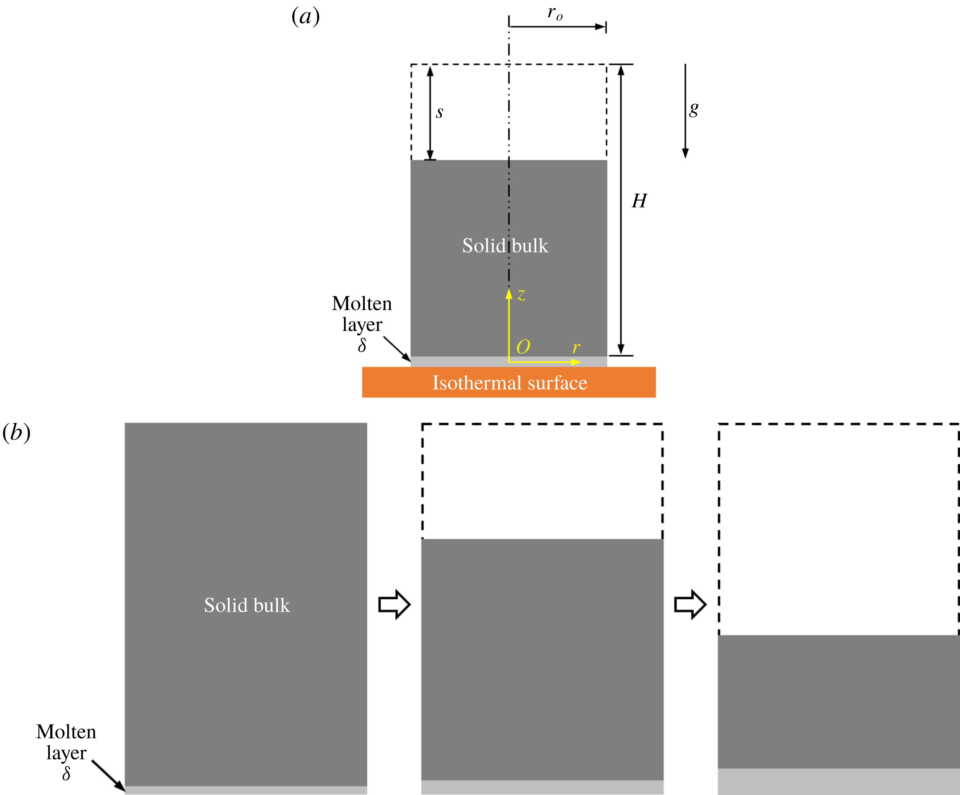
Basic schematics of the model and the transient melting process: (a) introduction of the main parameters used in the model, (b) qualitative demonstration of the transient close-contact melting process.

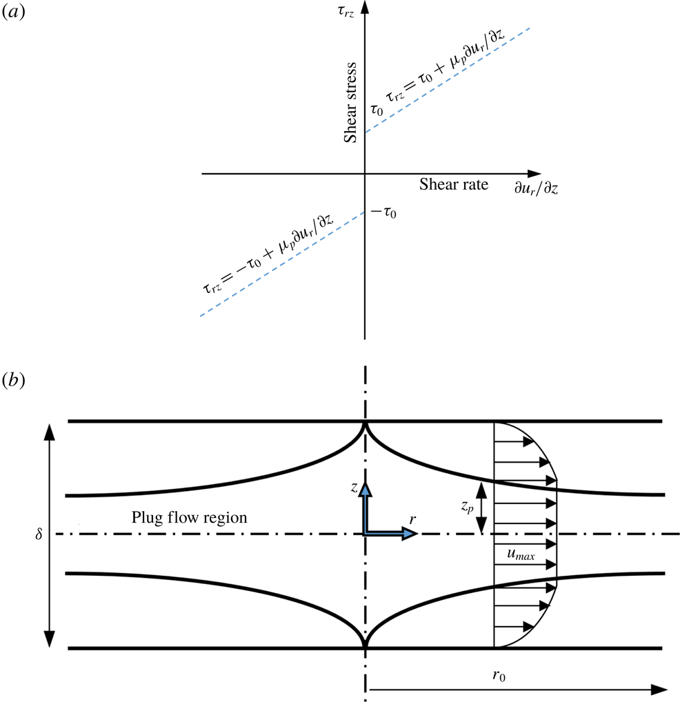
Schematics illustrating the non-Newtonian effects: (a) the shear stress as a function of the shear rate for a Bingham fluid, (b) the flow in the thin molten layer for a PCM with a liquid phase that behaves as a Bingham fluid.

2 Modelling the non-Newtonian effects
Although a model problem might be formulated as a two-dimensional (2-D) one in Cartesian coordinates, we analyse a more realistic axisymmetric case where the solid body is a vertical circular cylinder. The problem of a vertical cylinder that is melting directly on an isothermal surface has been studied experimentally and theoretically by Moallemi et al. (Reference Moallemi, Webb and Viskanta1986) and modelled also by Chen et al. (Reference Chen, Cheng, Luo and Gu1993) for the case where the solid is immersed in the liquid phase. General schematics of this model are depicted in figure 1(a) and a qualitative demonstration of the transient close-contact melting process is presented in figure 1(b). The results of these two studies showed that an analytical model for the melting rate can be devised under the following assumptions: (i) thin layer approximation, meaning that the thin molten layer thickness is much smaller than the cylinder radius, (ii) the upper solid interface remains flat, (iii) the effect of sensible heating is negligible, (iv) the flow in the thin molten layer is quasi-steady and laminar, (v) the liquid phase behaves as a Newtonian fluid, (vi) the solid bulk motion is quasi-steady, (vii) the effect of convection in the melt is negligible, (viii) the material is pure with constant properties, (ix) the pressure gradients are only in the radial direction. Regarding assumption (i), it can be shown by scaling analysis that for a sufficiently thin layer the
 $z$
-momentum equation can be neglected, and the
 $r$
-momentum equation is governed only by the balance between viscous and pressure forces, see for instance Ockendon & Ockendon (Reference Ockendon and Ockendon1995). The new model is formulated under the same assumptions, where only assumption (v) is now altered as the liquid phase is assumed to behave according to the Bingham model (Bingham Reference Bingham1916, Reference Bingham1922) for a non-Newtonian viscoplastic fluid, which is described as follows:
 $$\begin{eqnarray}\left.\begin{array}{@{}c@{}}\unicode[STIX]{x1D70F}_{rz}=\text{sign}\left({\displaystyle \frac{\unicode[STIX]{x2202}u_{r}}{\unicode[STIX]{x2202}z}}\right)\unicode[STIX]{x1D70F}_{0}+\unicode[STIX]{x1D707}_{p}{\displaystyle \frac{\unicode[STIX]{x2202}u_{r}}{\unicode[STIX]{x2202}z}},\quad |\unicode[STIX]{x1D70F}_{rz}|>\unicode[STIX]{x1D70F}_{0},\\ {\displaystyle \frac{\unicode[STIX]{x2202}u_{r}}{\unicode[STIX]{x2202}z}}=0,\quad |\unicode[STIX]{x1D70F}_{rz}|<\unicode[STIX]{x1D70F}_{0},\end{array}\right\}\end{eqnarray}$$
where
 $u_{r}$
is a velocity component in the radial direction,
 $\unicode[STIX]{x1D70F}_{rz}$
is the shear stress,
 $\unicode[STIX]{x1D70F}_{0}$
is the yield stress and
 $\unicode[STIX]{x1D707}_{p}$
is the plastic viscosity. A plot of (2.1) that presents the relation between the shear stress and shear rate is shown in figure 2(a). Although analysis of CCM of a liquid phase that behaves as a Bingham fluid has never been done before, this fluid was studied quite extensively in the past for similar regular single-phase flows. In a review paper by Bird et al. (Reference Bird, Dai and Yarusso1983), an analysis is presented of different flow configurations that are based on the thin layer approximation; in particular, a configuration of a radial flow between two disks is considered. This configuration has been studied numerically by Dai & Bird (Reference Dai and Bird1981) and analytically by Huang, Liu & Jiang (Reference Huang, Liu and Jiang1987). As the flow in the thin molten layer for a CCM of a vertical cylinder is very similar to this configuration, part of the current analysis is based on their results, especially those of Huang et al. (Reference Huang, Liu and Jiang1987), because their treatment of the problem is analytical. Another analysis that is also very similar to the current configuration was conducted by Covey & Stanmore (Reference Covey and Stanmore1981) for a radial squeeze flow of a Bingham fluid between two plates.
According to the analysis in these papers, the general physical principles of the problem will be described before stating its mathematical formulation. Then, some other physical considerations regarding applicability of the model will be discussed. First, the general schematics of the flow in the thin molten layer are depicted in figure 2(b). The molten layer thickness is denoted as
 $\unicode[STIX]{x1D6FF}$
and the cylinder’s outer radius is denoted as
 $r_{o}$
. It should be stressed that in order to present the problem details more clearly, this schematic diagram is drawn not to scale, as obviously according to the thin layer approximation
 $\unicode[STIX]{x1D6FF}\ll r_{o}$
. The coordinate system for the
 $r$
and
 $z$
directions is located at the centre of the thin molten layer, with respect to the two directions. One can see that the velocity profile is divided into two sections: a plug flow region and a regular shear flow region, where
 $z_{p}$
denotes the length in the
 $z$
-direction of the plug flow region from the molten layer thickness axis of symmetry at
 $z=0$
. This type of flow is typical for a Bingham fluid because as long as the shear stress is lower than the yield stress,
 $\unicode[STIX]{x1D70F}_{0}$
, the velocity gradient equals to zero and the fluid behaves as a rigid body, thus this region is characterized by a plug flow. Once the shear stress is higher than
 $\unicode[STIX]{x1D70F}_{0}$
, the velocity gradient attains a non-zero value. As the shear stress is always zero at the molten layer axis of symmetry, due to symmetry considerations, the plug flow region must be located around it. It is important to stress that the value of
 $z_{p}$
changes in the
 $r$
-direction and cannot be known a priori, and the schematic description of it as seen in figure 2(b) is based on the results of the analysis that will be presented below.
Some remarks should be added here about the applicability of the approach described above and utilized by Covey & Stanmore (Reference Covey and Stanmore1981) and Dai & Bird (Reference Dai and Bird1981). According to Lipscomb & Denn (Reference Lipscomb and Denn1984), the fluid in the plug flow region is considered as a rigid body and this type of flow is not possible kinematically, as the pressure gradient cannot lead to a constant velocity in the plug flow region. This issue has been resolved by Gartling & Phan-Thien (Reference Gartling and Phan-Thien1984) and Wilson (Reference Wilson1993) as they showed that the Bingham fluid model is a limiting case for the physically sound ‘biviscosity’ model. This model assumes that in the
 $\unicode[STIX]{x1D70F}_{0}>|\unicode[STIX]{x1D70F}_{rz}|$
region, the shear stress equals to the velocity gradient times a viscosity value that is higher than the plastic viscosity in region
 $\unicode[STIX]{x1D70F}_{0}<|\unicode[STIX]{x1D70F}_{rz}|$
. Gartling & Phan-Thien (Reference Gartling and Phan-Thien1984) showed that the Bingham fluid model gives an excellent approximation for the pressure gradient for the case where the viscosity ratio is very high. Thus, although the current model cannot capture the exact velocity profile, it does capture quite accurately the pressure gradient. Taking into account that the pressure gradient dictates the melting rate, which is the main interest of this study, this model should give a good approximation for both the melting time and molten layer thickness and also reveal the basic features of the problem. A more detailed investigation of the flow in the thin molten layer by utilizing the biviscosity model is possible for future studies but it is out of the scope of the current research.
After the main features and considerations of the suggested model have been discussed, the mathematical formulation of the problem can be stated. Accordingly, the momentum equation under the thin layer approximation for a general non-Newtonian fluid is:
 $$\begin{eqnarray}\frac{\text{d}p}{\text{d}r}=\frac{\unicode[STIX]{x2202}\unicode[STIX]{x1D70F}_{rz}}{\unicode[STIX]{x2202}z},\end{eqnarray}$$
where
 $p$
is pressure. Equation (2.2) can be easily integrated with respect to
 $z$
, as the pressure is assumed to vary only in the radial direction:
 $$\begin{eqnarray}\frac{\text{d}p}{\text{d}r}z=\unicode[STIX]{x1D70F}_{rz}+c_{1},\end{eqnarray}$$
where
 $c_{1}$
is an integration constant to be determined. The shear stress at the axis of symmetry is given by:
 $$\begin{eqnarray}\unicode[STIX]{x1D70F}_{rz}|_{z=0}=0.\end{eqnarray}$$
The constant
 $c_{1}$
can be determined by substituting (2.4) into (2.3) yielding the following result:
 $$\begin{eqnarray}c_{1}=0.\end{eqnarray}$$
Due to symmetry considerations, the analysis is performed only for the upper part of the thin molten layer flow. According to the Bingham model, the shear stress outside the plug flow region is given by:
 $$\begin{eqnarray}\unicode[STIX]{x1D70F}_{rz}=-\unicode[STIX]{x1D70F}_{0}+\unicode[STIX]{x1D707}_{p}\frac{\unicode[STIX]{x2202}u_{r}}{\unicode[STIX]{x2202}z}.\end{eqnarray}$$
Equations (2.5) and (2.6) can be substituted into (2.3), yielding the following relation:
 $$\begin{eqnarray}\frac{\text{d}p}{\text{d}r}z=-\unicode[STIX]{x1D70F}_{0}+\unicode[STIX]{x1D707}_{p}\frac{\unicode[STIX]{x2202}u_{r}}{\unicode[STIX]{x2202}z}.\end{eqnarray}$$
Equation (2.7) can be rearranged in order to yield the following expression for the velocity gradient:
 $$\begin{eqnarray}\frac{\unicode[STIX]{x2202}u_{r}}{\unicode[STIX]{x2202}z}=\frac{1}{\unicode[STIX]{x1D707}_{p}}\left(\frac{\text{d}p}{\text{d}r}z+\unicode[STIX]{x1D70F}_{0}\right).\end{eqnarray}$$
Integration of (2.8) with respect to
 $z$
yields the velocity distribution in the thin molten layer:
 $$\begin{eqnarray}u_{r}(z)=\frac{1}{\unicode[STIX]{x1D707}_{p}}\left(\frac{1}{2}\frac{\text{d}p}{\text{d}r}z^{2}+\unicode[STIX]{x1D70F}_{0}z\right)+c_{2},\end{eqnarray}$$
where
 $c_{2}$
is an integration constant that can be determined according to the following no-slip condition at the upper boundary of the thin molten layer:
 $$\begin{eqnarray}u_{r}(\unicode[STIX]{x1D6FF}/2)=0.\end{eqnarray}$$
Substitution of (2.10) into (2.9) yields the following result:
 $$\begin{eqnarray}c_{2}=-\frac{1}{\unicode[STIX]{x1D707}_{p}}\left(\frac{1}{2}\frac{\text{d}p}{\text{d}r}(\unicode[STIX]{x1D6FF}/2)^{2}+\unicode[STIX]{x1D70F}_{0}\unicode[STIX]{x1D6FF}/2\right).\end{eqnarray}$$
By substituting (2.11) back into (2.9), the velocity distribution outside the plug region can be found:
 $$\begin{eqnarray}u_{r}(z)=\frac{1}{2\unicode[STIX]{x1D707}_{p}}\frac{\text{d}p}{\text{d}r}[z^{2}-(\unicode[STIX]{x1D6FF}/2)^{2}]+\frac{\unicode[STIX]{x1D70F}_{0}}{\unicode[STIX]{x1D707}_{p}}[z-(\unicode[STIX]{x1D6FF}/2)],\quad z_{p}\leqslant z\leqslant \unicode[STIX]{x1D6FF}/2.\end{eqnarray}$$
The velocity in the plug region, which is denoted as
 $u_{max}$
, can be determined by substituting
 $z=z_{p}$
into (2.12):
 $$\begin{eqnarray}u_{r}(z_{p})=u_{max}=\frac{1}{2\unicode[STIX]{x1D707}_{p}}\frac{\text{d}p}{\text{d}r}[z_{p}^{2}-(\unicode[STIX]{x1D6FF}/2)^{2}]+\frac{\unicode[STIX]{x1D70F}_{0}}{\unicode[STIX]{x1D707}_{p}}[z_{p}-(\unicode[STIX]{x1D6FF}/2)],\quad 0\leqslant z\leqslant z_{p}.\end{eqnarray}$$
An expression for
 $z_{p}$
can be derived by using the fact that according to the Bingham model at
 $z=z_{p}$
, the velocity gradient should be zero, hence according to (2.8):
 $$\begin{eqnarray}\left.\frac{\unicode[STIX]{x2202}u_{r}}{\unicode[STIX]{x2202}z}\right|_{z=z_{p}}=\frac{1}{\unicode[STIX]{x1D707}_{p}}\frac{\text{d}p}{\text{d}r}z_{p}+\frac{\unicode[STIX]{x1D70F}_{0}}{\unicode[STIX]{x1D707}_{p}}=0.\end{eqnarray}$$
Equation (2.14) can be rearranged yielding the following expression for
 $z_{p}$
:
 $$\begin{eqnarray}z_{p}=\frac{-\unicode[STIX]{x1D70F}_{0}}{\text{d}p/\text{d}r}.\end{eqnarray}$$
Obviously, equation (2.15) implies that
 $z_{p}$
is inversely proportional to the pressure gradient and thus it varies in the
 $r$
-direction.
Equation (2.15) can now be substituted into (2.13), yielding the following expression for the velocity in the plug region:
 $$\begin{eqnarray}u_{max}=\frac{1}{2\unicode[STIX]{x1D707}_{p}}\frac{\text{d}p}{\text{d}r}\left[\left(\frac{-\unicode[STIX]{x1D70F}_{0}}{\text{d}p/\text{d}r}\right)^{2}-(\unicode[STIX]{x1D6FF}/2)^{2}\right]+\frac{\unicode[STIX]{x1D70F}_{0}}{\unicode[STIX]{x1D707}_{p}}\left[\frac{-\unicode[STIX]{x1D70F}_{0}}{\text{d}p/\text{d}r}-(\unicode[STIX]{x1D6FF}/2)\right],\quad 0\leqslant z\leqslant z_{p}.\end{eqnarray}$$
It is now possible to calculate the total volumetric flow rate,
 $Q$
, through integrating the velocity profiles and utilizing the symmetry of the flow as follows:
 $$\begin{eqnarray}Q=\int _{0}^{\unicode[STIX]{x1D6FF}}2\unicode[STIX]{x03C0}ru_{r}\,\text{d}z=2\int _{0}^{\unicode[STIX]{x1D6FF}/2}2\unicode[STIX]{x03C0}ru_{r}\,\text{d}z.\end{eqnarray}$$
Equations (2.12) and (2.16) can be substituted into (2.17) with the proper integration limits:
 $$\begin{eqnarray}Q=2\left\{\begin{array}{@{}c@{}}\displaystyle \int _{0}^{z_{p}}2\unicode[STIX]{x03C0}r\left({\displaystyle \frac{1}{2\unicode[STIX]{x1D707}_{p}}}{\displaystyle \frac{\text{d}p}{\text{d}r}}\left[\left({\displaystyle \frac{-\unicode[STIX]{x1D70F}_{0}}{\text{d}p/\text{d}r}}\right)^{2}-(\unicode[STIX]{x1D6FF}/2)^{2}\right]+{\displaystyle \frac{\unicode[STIX]{x1D70F}_{0}}{\unicode[STIX]{x1D707}_{p}}}\left[{\displaystyle \frac{-\unicode[STIX]{x1D70F}_{0}}{\text{d}p/\text{d}r}}-(\unicode[STIX]{x1D6FF}/2)\right]\right)\,\text{d}z\\ +\,\displaystyle \int _{z_{p}}^{\unicode[STIX]{x1D6FF}/2}2\unicode[STIX]{x03C0}r\left({\displaystyle \frac{1}{2\unicode[STIX]{x1D707}_{p}}}{\displaystyle \frac{\text{d}p}{\text{d}r}}[z^{2}-(\unicode[STIX]{x1D6FF}/2)^{2}]+{\displaystyle \frac{\unicode[STIX]{x1D70F}_{0}}{\unicode[STIX]{x1D707}_{p}}}[z-(\unicode[STIX]{x1D6FF}/2)]\right)\,\text{d}z\end{array}\right\}.\end{eqnarray}$$
Integration yields the following expression for the volumetric flow rate:
 $$\begin{eqnarray}Q=\frac{2\unicode[STIX]{x03C0}r}{\unicode[STIX]{x1D707}_{p}}\left\{\frac{1}{3}\unicode[STIX]{x1D70F}_{0}^{3}\left(\frac{\text{d}p}{\text{d}r}\right)^{-2}-\frac{1}{12}\unicode[STIX]{x1D6FF}^{3}\frac{\text{d}p}{\text{d}r}-\frac{1}{4}\unicode[STIX]{x1D6FF}^{2}\unicode[STIX]{x1D70F}_{0}\right\}.\end{eqnarray}$$
In order to derive an expression for the pressure gradient, the following dimensionless variable substitution is utilized (Huang et al. Reference Huang, Liu and Jiang1987):
 $$\begin{eqnarray}Z=-\frac{\text{d}r}{\text{d}p}\frac{\unicode[STIX]{x1D70F}_{0}}{\unicode[STIX]{x1D6FF}/2}.\end{eqnarray}$$
It should be noted that according to (2.15),
 $Z$
is actually
 $z_{p}$
normalized by half the thin molten layer thickness,
 $\unicode[STIX]{x1D6FF}/2$
. Thus, this variable is physically meaningful and can assume values between zero and unity. Substitution of (2.20) into (2.19) and some rearrangements yield the following cubic equation for
 $Z$
:
 $$\begin{eqnarray}Z^{3}-3\left(1+\frac{2\unicode[STIX]{x1D707}_{p}Q}{\unicode[STIX]{x03C0}r\unicode[STIX]{x1D6FF}^{2}\unicode[STIX]{x1D70F}_{0}}\right)Z+2=0.\end{eqnarray}$$
This result is identical to the analysis of Dai & Bird (Reference Dai and Bird1981); this equation can be solved for the pressure gradient as described in detail by Huang et al. (Reference Huang, Liu and Jiang1987), yielding the following expression:
 $$\begin{eqnarray}\frac{\text{d}p}{\text{d}r}=-\frac{\unicode[STIX]{x1D70F}_{0}}{\unicode[STIX]{x1D6FF}}\left(1+\frac{2\unicode[STIX]{x1D707}_{p}Q}{\unicode[STIX]{x03C0}\unicode[STIX]{x1D6FF}^{2}\unicode[STIX]{x1D70F}_{0}r}\right)^{-1/2}\text{sin}^{-1}\left(\frac{1}{3}\text{arcsin}\left[\left(1+\frac{2\unicode[STIX]{x1D707}_{p}Q}{\unicode[STIX]{x03C0}\unicode[STIX]{x1D6FF}^{2}\unicode[STIX]{x1D70F}_{0}r}\right)^{-3/2}\right]\right).\end{eqnarray}$$
The flow rate can be found according to the heat balance, as the heating rate equals the amount of molten material in the thin molten layer:
 $$\begin{eqnarray}\int _{0}^{r}-2\unicode[STIX]{x03C0}rk\left.\frac{\text{d}T}{\text{d}z}\right|_{z=-\unicode[STIX]{x1D6FF}/2}\,\text{d}r=\unicode[STIX]{x1D70C}_{l}L\int _{0}^{\unicode[STIX]{x1D6FF}}2\unicode[STIX]{x03C0}ru_{r}\,\text{d}z=\unicode[STIX]{x1D70C}_{l}LQ,\end{eqnarray}$$
where
 $T$
is temperature,
 $k$
is the liquid-phase thermal conductivity,
 $\unicode[STIX]{x1D70C}_{l}$
is the liquid-phase density and
 $L$
is the latent heat per unit mass. The temperature distribution in the thin molten layer can be obtained by solving the energy equation, using the thin layer approximation and the assumptions of a quasi-steady process with only heat conduction:
 $$\begin{eqnarray}\frac{\unicode[STIX]{x2202}^{2}T}{\unicode[STIX]{x2202}z^{2}}=0.\end{eqnarray}$$
The equation is solved with the following boundary conditions:
 $$\begin{eqnarray}\displaystyle & T(z=-\unicode[STIX]{x1D6FF}/2)=T_{w}, & \displaystyle\end{eqnarray}$$
 $$\begin{eqnarray}\displaystyle & T(z=\unicode[STIX]{x1D6FF}/2)=T_{m}, & \displaystyle\end{eqnarray}$$
where
 $T_{w}$
and
 $T_{m}$
are the hot surface and PCM melting temperatures, respectively. Its solution is given by the following linear relation as the heat transfer across the layer is assumed to be driven by heat conduction:
 $$\begin{eqnarray}T(z)=\frac{T_{m}-T_{w}}{\unicode[STIX]{x1D6FF}}z+\frac{T_{w}+T_{m}}{2}.\end{eqnarray}$$
Substitution of (2.27) into (2.23) and rearrangement yield the following expression for the volumetric flow rate in the thin molten layer:
 $$\begin{eqnarray}Q=\frac{\unicode[STIX]{x03C0}k(T_{w}-T_{m})}{\unicode[STIX]{x1D6FF}\unicode[STIX]{x1D70C}_{l}L}r^{2}.\end{eqnarray}$$
It should stressed that in the works by Dai & Bird (Reference Dai and Bird1981) and Huang et al. (Reference Huang, Liu and Jiang1987), the flow rate was assumed to be constant, whereas for the present case the flow rate is proportional to the square of the radial coordinate. However, the analysis above is still valid as no assumption regarding the flow rate distribution has been made. Due to this difference, from this point forth, this analysis diverges from the results presented in Huang et al. (Reference Huang, Liu and Jiang1987). Thus, equation (2.28) is substituted back into (2.22), yielding the following expression for the pressure gradient:
 $$\begin{eqnarray}\frac{\text{d}p}{\text{d}r}=-\frac{\unicode[STIX]{x1D70F}_{0}}{\unicode[STIX]{x1D6FF}}\left(1+\frac{2\unicode[STIX]{x1D707}_{p}k(T_{w}-T_{m})r}{\unicode[STIX]{x1D6FF}^{3}\unicode[STIX]{x1D70F}_{0}\unicode[STIX]{x1D70C}_{l}L}\right)^{-1/2}\text{sin}^{-1}\left(\frac{1}{3}\text{arcsin}\left[\left(1+\frac{2\unicode[STIX]{x1D707}_{p}k(T_{w}-T_{m})r}{\unicode[STIX]{x1D6FF}^{3}\unicode[STIX]{x1D70F}_{0}\unicode[STIX]{x1D70C}_{l}L}\right)^{-3/2}\right]\right).\end{eqnarray}$$
It should be noted that although for
 $\unicode[STIX]{x1D70F}_{0}=0$
this solution is singular, for
 $\unicode[STIX]{x1D70F}_{0}\rightarrow 0$
the pressure gradient converges to the classical solution for a Newtonian fluid (Moallemi et al.
Reference Moallemi, Webb and Viskanta1986). Also, based on (2.20), an explicit expression for
 $Z$
can be derived:
 $$\begin{eqnarray}Z=2\left(1+\frac{2\unicode[STIX]{x1D707}_{p}k(T_{w}-T_{m})r}{\unicode[STIX]{x1D6FF}^{3}\unicode[STIX]{x1D70F}_{0}\unicode[STIX]{x1D70C}_{l}L}\right)^{1/2}\text{sin}\left(\frac{1}{3}\text{arcsin}\left[\left(1+\frac{2\unicode[STIX]{x1D707}_{p}k(T_{w}-T_{m})r}{\unicode[STIX]{x1D6FF}^{3}\unicode[STIX]{x1D70F}_{0}\unicode[STIX]{x1D70C}_{l}L}\right)^{-3/2}\right]\right).\end{eqnarray}$$
The next step is to integrate the pressure gradient in order to derive the pressure distribution in the thin molten layer. This can be done by following the technique, presented in Huang et al. (Reference Huang, Liu and Jiang1987) for a constant flow rate. First, equation (2.28) for the flow rate is substituted into (2.21) and rearranged in order to isolate
 $r$
:
 $$\begin{eqnarray}r=\frac{\unicode[STIX]{x1D6FF}^{3}\unicode[STIX]{x1D70C}_{l}L\unicode[STIX]{x1D70F}_{0}}{6\unicode[STIX]{x1D707}_{p}k(T_{w}-T_{m})}\left(Z^{2}+\frac{2}{Z}-3\right)=F(Z).\end{eqnarray}$$
Equation (2.31) implies that
 $r$
is related to
 $Z$
that is denoted as
 $F(Z)$
, and can be differentiated with respect to
 $Z$
and, by applying the chain rule and substituting the inverse pressure gradient that can be derived from (2.20), the following relation can be found:
 $$\begin{eqnarray}F^{\prime }(Z)=\frac{\text{d}r}{\text{d}Z}=\frac{\text{d}r}{\text{d}p}\frac{\text{d}p}{\text{d}Z}=-\frac{\unicode[STIX]{x1D6FF}/2}{\unicode[STIX]{x1D70F}_{0}}Z\frac{\text{d}p}{\text{d}Z}.\end{eqnarray}$$
It is now possible to isolate the pressure differential, integrate both sides of the equation and substitute the explicit form of the derivative of
 $F$
(
 $Z$
), see (2.31); this yields an expression for the pressure distribution in the thin molten layer:
 $$\begin{eqnarray}\displaystyle p & = & \displaystyle -\frac{\unicode[STIX]{x1D70F}_{0}}{\unicode[STIX]{x1D6FF}/2}\int \frac{F^{\prime }(Z)}{Z}\,\text{d}Z=-\frac{\unicode[STIX]{x1D70F}_{0}}{\unicode[STIX]{x1D6FF}/2}\int \frac{{\displaystyle \frac{\unicode[STIX]{x1D6FF}^{3}\unicode[STIX]{x1D70C}_{l}L\unicode[STIX]{x1D70F}_{0}}{6\unicode[STIX]{x1D707}_{p}k(T_{w}-T_{m})}}\left(2Z-{\displaystyle \frac{2}{Z^{2}}}\right)}{Z}\,\text{d}Z\nonumber\\ \displaystyle & = & \displaystyle -\frac{\unicode[STIX]{x1D6FF}^{2}\unicode[STIX]{x1D70C}_{l}L\unicode[STIX]{x1D70F}_{0}^{2}}{3\unicode[STIX]{x1D707}_{p}k(T_{w}-T_{m})}\left(2Z+\frac{1}{Z^{2}}\right)+C,\end{eqnarray}$$
where
 $C$
is an integration constant to be determined. This constant can be found by applying the following zero gauge pressure boundary condition at the outlet of the thin molten layer:
 $$\begin{eqnarray}p(r_{o}=0)=0.\end{eqnarray}$$
In principle, the value of pressure at the outlet should not change the solution as the flow is driven by the pressure difference, which remains the same regardless of the pressure outlet value. The zero gauge pressure outlet was chosen in order to simplify the equations. Thus, by substituting (2.34) into (2.33),
 $C$
is given as:
 $$\begin{eqnarray}C=\frac{\unicode[STIX]{x1D6FF}^{2}\unicode[STIX]{x1D70C}_{l}L\unicode[STIX]{x1D70F}_{0}^{2}}{3\unicode[STIX]{x1D707}_{p}k(T_{w}-T_{m})}\left(2Z_{o}+\frac{1}{Z_{o}^{2}}\right),\end{eqnarray}$$
where
 $Z_{o}$
is defined as
 $Z$
(
 $r=r_{o}$
). Thus, according to (2.30),
 $Z_{o}$
is given by the following expression:
 $$\begin{eqnarray}Z_{o}=2\left(1+\frac{2\unicode[STIX]{x1D707}_{p}k(T_{w}-T_{m})r_{o}}{\unicode[STIX]{x1D6FF}^{3}\unicode[STIX]{x1D70F}_{0}\unicode[STIX]{x1D70C}_{l}L}\right)^{1/2}\text{sin}\left(\frac{1}{3}\text{arcsin}\left[\left(1+\frac{2\unicode[STIX]{x1D707}_{p}k(T_{w}-T_{m})r_{o}}{\unicode[STIX]{x1D6FF}^{3}\unicode[STIX]{x1D70F}_{0}\unicode[STIX]{x1D70C}_{l}L}\right)^{-3/2}\right]\right).\end{eqnarray}$$
Equation (2.35) can be substituted back into (2.33) to yield an analytical expression for the pressure distribution in the thin molten layer:
 $$\begin{eqnarray}p=-\frac{\unicode[STIX]{x1D6FF}^{2}\unicode[STIX]{x1D70C}_{l}L\unicode[STIX]{x1D70F}_{0}^{2}}{3\unicode[STIX]{x1D707}_{p}k(T_{w}-T_{m})}\left(2Z+\frac{1}{Z^{2}}-2Z_{o}-\frac{1}{Z_{o}^{2}}\right)=\,f(Z).\end{eqnarray}$$
One can see that the pressure is a function of
 $Z$
and thus it is denoted as
 $f$
(
 $Z$
).
Now since the pressure distribution is known explicitly, it can be integrated in order to obtain the total force that is exerted on the solid bulk due to the pressure in the thin molten layer. First of all, the following differential relation can be easily derived from (2.20):
 $$\begin{eqnarray}\text{d}r=-\frac{\unicode[STIX]{x1D6FF}/2}{\unicode[STIX]{x1D70F}_{0}}Z\,\text{d}p.\end{eqnarray}$$
Secondly, the pressure differential can be calculated as a function of
 $Z$
, following the notation used in (2.37):
 $$\begin{eqnarray}\text{d}p=f^{\prime }(Z)\,\text{d}Z.\end{eqnarray}$$
Substitution of (2.39) into (2.38) yields the following differential relation between
 $r$
and
 $Z$
:
 $$\begin{eqnarray}\text{d}r=-\frac{\unicode[STIX]{x1D6FF}/2}{\unicode[STIX]{x1D70F}_{0}}Zf^{\prime }(Z)\,\text{d}Z.\end{eqnarray}$$
Equations (2.31), (2.37) and (2.40) can now be substituted into the force balance expression in order to yield an integral with respect to
 $Z$
. The integral limits are altered accordingly as
 $Z(r=0)=$
1 and
 $Z(r=r_{o})=Z_{o}$
:
 $$\begin{eqnarray}\int _{0}^{r_{o}}2\unicode[STIX]{x03C0}rp\,\text{d}r=-\frac{\unicode[STIX]{x1D6FF}/2}{\unicode[STIX]{x1D70F}_{0}}2\unicode[STIX]{x03C0}\int _{1}^{Z_{o}}F(Z)f(Z)Zf^{\prime }(Z)\,\text{d}Z.\end{eqnarray}$$
After substitution of the explicit expressions for all the associated functions, see (2.31) and (2.37), and some rearrangements, the following expression can be derived:
 $$\begin{eqnarray}\displaystyle \int _{0}^{r_{o}}2\unicode[STIX]{x03C0}rp\,\text{d}r & = & \displaystyle -2\unicode[STIX]{x03C0}\left(\frac{\unicode[STIX]{x1D6FF}^{3}\unicode[STIX]{x1D70C}_{l}L\unicode[STIX]{x1D70F}_{0}}{6\unicode[STIX]{x1D707}_{p}k(T_{w}-T_{m})}\right)^{3}\frac{\unicode[STIX]{x1D70F}_{0}}{\unicode[STIX]{x1D6FF}/2}\nonumber\\ \displaystyle & & \displaystyle \times \,\int _{1}^{Z_{o}}\left(Z^{2}+\frac{2}{Z}-3\right)\left(2Z+\frac{1}{Z^{2}}-2Z_{o}-\frac{1}{Z_{o}^{2}}\right)\left(2Z-\frac{2}{Z^{2}}\right)\,\text{d}Z.\quad \qquad\end{eqnarray}$$
Integration leads to the following analytical expression for the force exerted on the solid bulk by the thin molten layer:
 $$\begin{eqnarray}\displaystyle \int _{0}^{r_{o}}2\unicode[STIX]{x03C0}rp\,\text{d}r & = & \displaystyle -2\unicode[STIX]{x03C0}\left(\frac{\unicode[STIX]{x1D6FF}^{3}\unicode[STIX]{x1D70C}_{l}L\unicode[STIX]{x1D70F}_{0}}{6\unicode[STIX]{x1D707}_{p}k(T_{w}-T_{m})}\right)^{3}\frac{\unicode[STIX]{x1D70F}_{0}}{\unicode[STIX]{x1D6FF}/2}\nonumber\\ \displaystyle & & \displaystyle \times \left(\frac{51}{5}-\frac{1}{Z_{o}^{4}}+\frac{4}{Z_{o}^{3}}-\frac{9}{2Z_{o}^{2}}-9Z_{o}-\frac{3Z_{o}^{2}}{2}+2Z_{o}^{3}-\frac{Z_{o}^{5}}{5}+6\text{ln}Z_{o}\right)\!.\quad \qquad\end{eqnarray}$$
It is now possible to equate (2.43) with the time-dependent solid bulk weight:
 $$\begin{eqnarray}\displaystyle & & \displaystyle -2\unicode[STIX]{x03C0}\left(\frac{\unicode[STIX]{x1D6FF}^{3}\unicode[STIX]{x1D70C}_{l}L\unicode[STIX]{x1D70F}_{0}}{6\unicode[STIX]{x1D707}_{p}k(T_{w}-T_{m})}\right)^{3}\frac{\unicode[STIX]{x1D70F}_{0}}{\unicode[STIX]{x1D6FF}/2}\nonumber\\ \displaystyle & & \displaystyle \qquad \times \left(\frac{51}{5}-\frac{1}{Z_{o}^{4}}+\frac{4}{Z_{o}^{3}}-\frac{9}{2Z_{o}^{2}}-9Z_{o}-\frac{3Z_{o}^{2}}{2}+2Z_{o}^{3}-\frac{Z_{o}^{5}}{5}+6\text{ln}Z_{o}\right)\nonumber\\ \displaystyle & & \displaystyle \quad =g\unicode[STIX]{x1D70C}_{s}\unicode[STIX]{x03C0}r_{o}^{2}(H-s),\end{eqnarray}$$
where
 $\unicode[STIX]{x1D70C}_{s}$
is the solid-phase density,
 $g$
is the gravitational acceleration,
 $H$
is the cylinder’s initial height and
 $s$
is the solid upper surface location. Equation (2.44) provides a relation between the molten layer thickness,
 $\unicode[STIX]{x1D6FF}$
, and the solid upper surface descent,
 $s$
. It should be noted that
 $Z_{o}$
is also dependent on
 $\unicode[STIX]{x1D6FF}$
in a rather complex relation, see (2.36). Hence, equation (2.44) is a nonlinear algebraic equation for
 $\unicode[STIX]{x1D6FF}$
, and its value can be derived for each value of
 $s$
. Although the entire treatment to this point is analytical, equation (2.44) is solved numerically, as no analytical solution can be derived. In order to calculate the solid descent velocity, the Stefan condition is applied:
 $$\begin{eqnarray}\unicode[STIX]{x1D70C}_{s}L\frac{\text{d}s}{\text{d}t}=-k\left.\frac{\text{d}T}{\text{d}z}\right|_{z=-\unicode[STIX]{x1D6FF}/2}.\end{eqnarray}$$
The temperature distribution, equation (2.27), can be substituted into (2.45) yielding the following relation between the molten layer thickness,
 $\unicode[STIX]{x1D6FF}$
, and the solid descent velocity,
 $\text{d}s/\text{d}t$
:
 $$\begin{eqnarray}\unicode[STIX]{x1D70C}_{s}L\frac{\text{d}s}{\text{d}t}=k\frac{T_{w}-T_{m}}{\unicode[STIX]{x1D6FF}}.\end{eqnarray}$$
Equation (2.46) can be discretized by using the forward Euler method yielding the following numerical scheme:
 $$\begin{eqnarray}s^{n+1}=s^{n}+\frac{k(T_{w}-T_{m})}{\unicode[STIX]{x1D6FF}^{n}\unicode[STIX]{x1D70C}_{s}L}\unicode[STIX]{x0394}t,\end{eqnarray}$$
where
 $\unicode[STIX]{x0394}t$
is the size of the time step, and the superscripts
 $n$
and
 $n+1$
denote the variables’ values at the current and next time step, respectively. The problem is solved with the following initial condition:
 $$\begin{eqnarray}s(t=0)=0.\end{eqnarray}$$
The numerical procedure first involves solution of (2.44) using
 $s^{n}$
, which is the value of
 $s$
at the current time step, this allows deriving
 $\unicode[STIX]{x1D6FF}^{n}$
. Then, these values are used to calculate
 $s^{n+1}$
with the numerical scheme that is described in (2.47). This procedure continues until almost total melting of the solid is reached, meaning that
 $s^{n+1}\approx H$
, see figure 1. Although this procedure is quite simple and straightforward, there are some technical difficulties in numerically estimating the left-hand side of (2.44) for relatively high values of
 $\unicode[STIX]{x1D6FF}$
and
 $\unicode[STIX]{x1D70F}_{0}$
. The reason for this difficulty and its solution will be illustrated next, and it will be shown that the solution for this issue actually allows obtaining a reduced model that can be solved analytically, and sheds some light on the physical processes that are involved. First, we may note that according to (2.36),
 $Z_{o}$
is actually a function of a single dimensionless group that will be denoted as
 $\unicode[STIX]{x1D700}$
:
 $$\begin{eqnarray}\unicode[STIX]{x1D700}=\frac{2\unicode[STIX]{x1D707}_{p}k(T_{w}-T_{m})r_{o}}{\unicode[STIX]{x1D6FF}^{3}\unicode[STIX]{x1D70F}_{0}\unicode[STIX]{x1D70C}_{l}L}.\end{eqnarray}$$
Accordingly, equation (2.36) assumes the following form:
 $$\begin{eqnarray}Z_{o}=2(1+\unicode[STIX]{x1D700})^{1/2}\text{sin}\left({\textstyle \frac{1}{3}}\text{arcsin}[(1+\unicode[STIX]{x1D700})^{-3/2}]\right).\end{eqnarray}$$
By using this definition of
 $\unicode[STIX]{x1D700}$
, it is possible to rearrange (2.44) into the following form:
 $$\begin{eqnarray}-\frac{4}{27}\frac{\unicode[STIX]{x1D70F}_{0}r_{0}}{\unicode[STIX]{x1D6FF}}G(\unicode[STIX]{x1D700})=g\unicode[STIX]{x1D70C}_{s}(H-s),\end{eqnarray}$$
where
 $G(\unicode[STIX]{x1D700})$
is a function of only
 $\unicode[STIX]{x1D700}$
, and it is given by the following expression:
 $$\begin{eqnarray}G(\unicode[STIX]{x1D700})=\left.\left(\frac{51}{5}-\frac{1}{Z_{o}^{4}}+\frac{4}{Z_{o}^{3}}-\frac{9}{2Z_{o}^{2}}-9Z_{o}-\frac{3Z_{o}^{2}}{2}+2Z_{o}^{3}-\frac{Z_{o}^{5}}{5}+6\text{ln}Z_{o}\right)\right/\unicode[STIX]{x1D700}^{3}.\end{eqnarray}$$
The form of
 $G(\unicode[STIX]{x1D700})$
reveals the problem of numerically estimating its value. For low values of
 $\unicode[STIX]{x1D700}$
that correspond to high values of
 $\unicode[STIX]{x1D6FF}$
and
 $\unicode[STIX]{x1D70F}_{0}$
, expressions in both the numerator and denominator tend to zero. Numerical estimation of
 $G(\unicode[STIX]{x1D700})$
is thus rather difficult, as for low values of
 $\unicode[STIX]{x1D700}$
the round-off errors in both the expressions in the numerator and denominator tend to dominate and make the estimation of
 $G(\unicode[STIX]{x1D700})$
impossible. However, it turns out that it is possible to calculate the value of
 $G(\unicode[STIX]{x1D700})$
in the limiting case of
 $\unicode[STIX]{x1D700}\rightarrow 0$
, thus:
 $$\begin{eqnarray}\text{lim}_{\unicode[STIX]{x1D700}\rightarrow 0}G(\unicode[STIX]{x1D700})=-{\textstyle \frac{9}{2}}.\end{eqnarray}$$
Obviously, for sufficiently low values of
 $\unicode[STIX]{x1D700}$
this limit can provide a reasonable estimation of
 $G(\unicode[STIX]{x1D700})$
. By comparing this estimation with numerical integration of the pressure gradient, which does not suffer from this issue, it was found that for values of
 $\unicode[STIX]{x1D700}$
that are lower than
 $0.5\times 10^{-4}$
, the use of this limit for estimation of the function
 $G(\unicode[STIX]{x1D700})$
leads to an error of less than 1 %. According to this analysis, during the numerical solution of the problem, this estimation is utilized for values of
 $\unicode[STIX]{x1D700}$
that are lower than
 $0.5\times 10^{-4}$
. One may note that the value of
 $\unicode[STIX]{x1D700}$
decreases with time because the molten layer thickness,
 $\unicode[STIX]{x1D6FF}$
, increases with time due to the decrease in the solid bulk weight as the melting progresses. It is thus possible that this estimation can be quite a reasonable approximation for assessing the melting rate. In order to test this approach, equation (2.53) can be substituted into (2.44):
 $$\begin{eqnarray}-\frac{4}{27}\frac{\unicode[STIX]{x1D70F}_{0}r_{0}}{\unicode[STIX]{x1D6FF}}\left(-\frac{9}{2}\right)=g\unicode[STIX]{x1D70C}_{s}(H-s).\end{eqnarray}$$
According to (2.46),
 $\unicode[STIX]{x1D6FF}$
is given by the following relation:
 $$\begin{eqnarray}\unicode[STIX]{x1D6FF}=k\frac{T_{w}-T_{m}}{L\unicode[STIX]{x1D70C}_{s}{\displaystyle \frac{\text{d}s}{\text{d}t}}}.\end{eqnarray}$$
After substitution of (2.55) into (2.54) and some rearrangements, the following ordinary first-order differential equation for
 $s$
can be derived:
 $$\begin{eqnarray}\frac{\text{d}s}{\text{d}t}=\frac{3}{2}\frac{gk(T_{w}-T_{m})}{r_{o}L\unicode[STIX]{x1D70F}_{0}}(H-s).\end{eqnarray}$$
This equation can be integrated and solved analytically:
 $$\begin{eqnarray}\int _{0}^{s}\frac{\text{d}s}{H-s}=\frac{3}{2}\frac{gk(T_{w}-T_{m})}{r_{o}L\unicode[STIX]{x1D70F}_{0}}\int _{0}^{t}\,\text{d}t.\end{eqnarray}$$
The solution for the time-dependent upper surface of the solid location,
 $s$
, is given by the following expression:
 $$\begin{eqnarray}s(t)=H\left(1-\text{exp}\left[-\frac{3}{2}\frac{gk(T_{w}-T_{m})}{r_{o}L\unicode[STIX]{x1D70F}_{0}}t\right]\right).\end{eqnarray}$$
This relation can be divided by
 $H$
in order to yield an expression for the melt fraction as a function of time:
 $$\begin{eqnarray}\frac{s(t)}{H}=1-\text{exp}\left[-\frac{3}{2}\frac{gk(T_{w}-T_{m})}{r_{o}L\unicode[STIX]{x1D70F}_{0}}t\right].\end{eqnarray}$$
Substitution of (2.58) into (2.54) also yields an analytical expression for the molten layer thickness,
 $\unicode[STIX]{x1D6FF}$
, as a function of time:
 $$\begin{eqnarray}\unicode[STIX]{x1D6FF}=\frac{2}{3}\frac{r_{o}\unicode[STIX]{x1D70F}_{0}}{g\unicode[STIX]{x1D70C}_{s}H}\text{exp}\left[\frac{3}{2}\frac{gk(T_{w}-T_{m})}{r_{o}L\unicode[STIX]{x1D70F}_{0}}t\right].\end{eqnarray}$$
The present approximate analysis reveals some interesting features of the problem. First of all, it shows that at some point in the melting process both the melt fraction and molten layer thickness start to vary exponentially. Secondly, it seems that at least theoretically, the total melting time in the case of a Bingham fluid is infinite as opposed to the Newtonian classical solution where the total melting time is finite. This proves that the non-Newtonian behaviour of the liquid phase can decrease the melting rate. Third, quite interestingly, for this limiting case, the melting rate does not depend on the plastic viscosity,
 $\unicode[STIX]{x1D707}_{p}$
, or either the solid- or liquid-phase densities,
 $\unicode[STIX]{x1D70C}_{s}$
and
 $\unicode[STIX]{x1D70C}_{l}$
, respectively. Taking into account that for this limiting case
 $Z_{o}=1$
, which implies that at the outlet of the thin molten layer
 $z_{p}=\unicode[STIX]{x1D6FF}/2$
, meaning that the entire velocity profile behaves as a plug flow, the fact that this approximation does not depend on the plastic viscosity makes sense, see (2.36).
Another interesting limiting case is
 $\unicode[STIX]{x1D700}\gg 1$
, where the yield stress,
 $\unicode[STIX]{x1D70F}_{0}$
, is typically low. It seems that in this limit, the function
 $G$
(
 $\unicode[STIX]{x1D700}$
) is well approximated by the following relation:
 $$\begin{eqnarray}G(\unicode[STIX]{x1D700})=-{\textstyle \frac{81}{16}}\unicode[STIX]{x1D700}.\end{eqnarray}$$
Not surprisingly, substitution of (2.61) into (2.51) yields an expression which is independent of
 $\unicode[STIX]{x1D70F}_{0}$
. It is easy to show that by substituting (2.55) into this expression and solving for
 $s$
, the classical analytical solution for a Newtonian fluid that was first derived by Moallemi et al. (Reference Moallemi, Webb and Viskanta1986) can be reproduced.
Dimensional analysis. Some features of the current problem can be revealed by dimensional analysis. First, it is possible to derive some of the governing dimensionless groups of the problem by using the analytical approximation results. Accordingly, equations (2.59) and (2.60) can be rendered into dimensionless form:
 $$\begin{eqnarray}\displaystyle & \displaystyle \frac{s}{H}=1-\text{exp}\left[-\frac{3}{2}\frac{SteFo}{\unicode[STIX]{x1D6FA}\unicode[STIX]{x1D70C}_{\ast }}\right], & \displaystyle\end{eqnarray}$$
 $$\begin{eqnarray}\displaystyle & \displaystyle \frac{\unicode[STIX]{x1D6FF}}{H}=\frac{2}{3}\unicode[STIX]{x1D6FA}\text{exp}\left[\frac{3}{2}\frac{SteFo}{\unicode[STIX]{x1D6FA}\unicode[STIX]{x1D70C}_{\ast }}\right], & \displaystyle\end{eqnarray}$$
where the dimensionless groups that govern the problem include the Stefan and Fourier numbers and are defined as follows:
 $$\begin{eqnarray}Ste=\frac{c_{p}(T_{w}-T_{m})}{L},\quad Fo=\frac{\unicode[STIX]{x1D6FC}_{l}t}{H^{2}},\quad \unicode[STIX]{x1D70C}_{\ast }=\frac{\unicode[STIX]{x1D70C}_{s}}{\unicode[STIX]{x1D70C}_{l}},\quad \unicode[STIX]{x1D6FA}=\frac{r_{o}\unicode[STIX]{x1D70F}_{0}}{g\unicode[STIX]{x1D70C}_{s}H^{2}},\end{eqnarray}$$
where
 $c_{p}$
is specific heat capacity, and
 $\unicode[STIX]{x1D6FC}_{l}$
is the liquid-phase thermal diffusivity. This analysis indicates that the melt fraction is a function of a single dimensionless group,
 $SteFo/(\unicode[STIX]{x1D6FA}\unicode[STIX]{x1D70C}_{\ast })$
, and that the dimensionless molten layer thickness is a function of two dimensionless groups,
 $SteFo/(\unicode[STIX]{x1D6FA}\unicode[STIX]{x1D70C}_{\ast })$
and
 $\unicode[STIX]{x1D6FA}$
.
An analysis of the exact solution is more difficult as there is no explicit analytical expression that can reveal the dependence of the dimensionless groups on the parameters of interest. However, the dimensionless groups that govern the problem can be found according to (2.51) that is rendered into dimensionless form:
 $$\begin{eqnarray}-\frac{4}{27}\frac{\unicode[STIX]{x1D6FA}\unicode[STIX]{x1D70C}_{\ast }}{Ste}\frac{\text{d}s_{\ast }}{\text{d}Fo}G(\unicode[STIX]{x1D700})=1-s_{\ast },\end{eqnarray}$$
where
 $s_{\ast }=s/H$
, which actually is the melt fraction. Equation (2.65) suggests that the melt fraction,
 $s_{\ast }$
, depends on
 $SteFo/(\unicode[STIX]{x1D6FA}\unicode[STIX]{x1D70C}_{\ast })$
. This dimensionless group was already introduced through the scrutiny of the analytical solution. However, equation (2.65) also includes a dimensionless group that depends on
 $s_{\ast }$
, namely,
 $\unicode[STIX]{x1D700}$
. In order to analyse this dimensionless group, equation (2.55) can be substituted into (2.49), and after some rearrangements the following expression for
 $\unicode[STIX]{x1D700}$
can be derived:
 $$\begin{eqnarray}\unicode[STIX]{x1D700}=2\left(\frac{\unicode[STIX]{x1D70C}_{\ast }}{Pr^{1/3}He^{1/3}Ste^{2/3}}\frac{r_{o}}{H}\frac{\text{d}s_{\ast }}{\text{d}Fo}\right)^{3},\end{eqnarray}$$
where two additional dimensionless groups are introduced:
 $$\begin{eqnarray}\left.\begin{array}{@{}c@{}}\text{the Prandtl number }Pr={\displaystyle \frac{\unicode[STIX]{x1D708}}{\unicode[STIX]{x1D6FC}_{l}}},\\ \text{the Hedstrom number }He={\displaystyle \frac{\unicode[STIX]{x1D70C}_{l}r_{o}^{2}\unicode[STIX]{x1D70F}_{0}}{\unicode[STIX]{x1D707}_{p}^{2}}},\end{array}\right\}\end{eqnarray}$$
where
 $\unicode[STIX]{x1D708}$
is kinematic viscosity. Thus, according to (2.65) and (2.66), it can be deduced that the melt fraction,
 $s_{\ast }$
, is a function of two dimensionless groups:
 $$\begin{eqnarray}s_{\ast }=f\left(\frac{\unicode[STIX]{x1D6FA}\unicode[STIX]{x1D70C}_{\ast }}{SteFo},\frac{\unicode[STIX]{x1D70C}_{\ast }}{Pr^{1/3}He^{1/3}Ste^{2/3}Fo}\frac{r_{o}}{H}\right).\end{eqnarray}$$
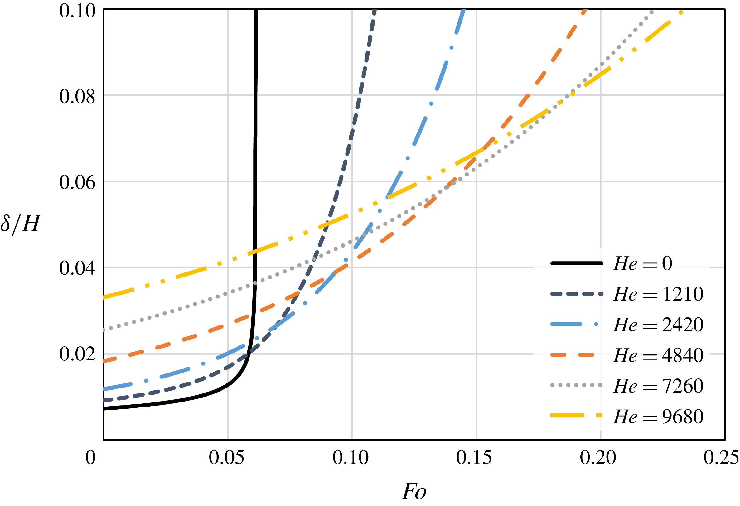
The molten layer thickness as a function of time, for different Hedstrom numbers,
 $He=0$
, 1210, 2420, 4840, 7260 and 9680.

3 Results and discussion
It is of interest to study the effect of the yield stress,
 $\unicode[STIX]{x1D70F}_{0}$
, on both the melting rate and the molten layer thickness and compare the results with the classical Newtonian solution where
 $\unicode[STIX]{x1D70F}_{0}=0$
. All the reported results are presented in dimensionless form, based on the properties of eicosane (
 $\text{C}_{20}\text{H}_{42}$
), where the exact property values used in this work can be found in Kozak et al. (Reference Kozak, Rozenfeld and Ziskind2014). The temperature difference between the hot isothermal surface and the PCM melting temperature is assumed to be
 $20\,^{\circ }\text{C}$
, and the cylinder’s initial height and diameter are chosen to be 10 mm. Different values of the Hedstrom number are investigated: 0, 1210, 2420, 4840, 7260 and 9680, which correspond to
 $\unicode[STIX]{x1D70F}_{0}$
values of 0, 1, 2, 4, 6 and 8 Pa, respectively. We note that although liquid eicosane is a Newtonian fluid, there are indications that non-Newtonian effects in it might be induced by nanoinclusions, although at this stage, we do not intend to deal with that issue and the effective properties induced by the nanoparticles are not taken into account. This is done in order to test the basic features of the new model without adding any further complicating effects.
Figure 3 shows the normalized molten layer thickness,
 $\unicode[STIX]{x1D6FF}/H$
, as a function of the
 $Fo$
number for different values of the
 $He$
number. It is easy to see that at the initial stages of melting, the molten layer is thicker as the yield stress increases. In fact, if the same melt fractions are compared, the molten layer thickness is always greater for a higher yield stress. Also, for the Newtonian case, at the initial stages of the melting, the thickness increases at a much slower rate than in the non-Newtonian cases, and only at the very last stages it increases abruptly. One may note that the current results are presented up to a normalized thickness of 0.1. This value represents a rough estimate of a thickness where the thin layer approximation does not hold, as according to assumption (i)
 $\unicode[STIX]{x1D6FF}\ll r_{o}$
. For this value the current model prediction is unreliable and a full solution of the momentum equations for the molten layer is necessary. Thus, the results are presented up to this value. It is obvious that a thicker molten layer creates a higher thermal resistance which reduces the heat transfer rates and thus the melting rate.
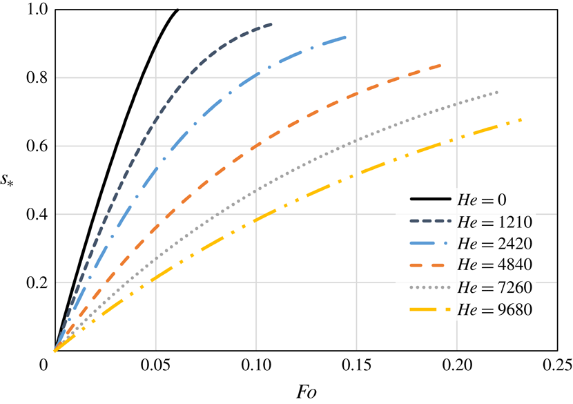
This can be seen in figure 4, which shows the melt fraction as a function of the
 $Fo$
number for different
 $He$
numbers. As explained above, due to the increase in the thin molten layer thickness, the melting rate decreases as the yield stress increases. This effect is very significant for the values of the yield stress that are examined. The melt fraction curves are presented up to the value where the normalized molten layer thickness reaches a value of 0.1, due to the reasons explained above. As the yield stress increases, the value of the melt fraction at which the current model prediction becomes unacceptable decreases. It is obvious that up to this stage, the non-Newtonian effects can decrease the melting rate significantly. This clearly shows that a PCM that behaves as a Newtonian fluid will finish its melting process long before these stages are reached for a PCM that behaves as a Bingham fluid.
The melt fraction as a function of time, for different Hedstrom numbers,
 $He=0$
, 1210, 2420, 4840, 7260 and 9680.

Comparison between the exact numerical model and the analytical approximation: (a) molten layer thickness,
 $He=1210$
, (b) melt fraction,
 $He=1210$
, (c) molten layer thickness,
 $He=2420$
, (d) melt fraction,
 $He=2420$
, (e) molten layer thickness,
 $He=4840$
, (f) melt fraction,
 $He=4840$
, (g) molten layer thickness,
 $He=7260$
, (h) melt fraction,
 $He=7260$
, (i) molten layer thickness,
 $He=9680$
, (j) melt fraction,
 $He=9680$
.

Contours of the melt fraction,
 $s_{\ast }$
, as a function of the dimensionless groups,
 $SteFo/(\unicode[STIX]{x1D6FA}\unicode[STIX]{x1D70C}_{\ast })$
and
 $(H/r_{o})\,Pr^{1/3}He^{1/3}Ste^{2/3}Fo/\unicode[STIX]{x1D70C}_{\ast }$
, for different Hedstrom numbers,
 $He=1210$
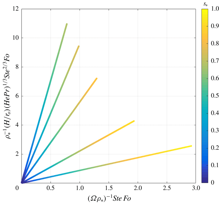
, 2420, 4840, 7260 and 9680 (counterclockwise order).

It is now possible to compare the results with the reduced analytical model, where its predictions for the melt fraction and normalized molten layer thickness are given by (2.59) and (2.60), respectively. Figure 5(a) compares the molten layer thickness according to the numerical model and the analytical approximation for
 $He=1210$
. It can be seen that at the initial stages of the melting, the approximate approach under-predicts the normalized molten layer thickness and at later stages over-predicts it. The errors are quite large and it seems that this approximation is not acceptable for this case. A comparison for the predictions of the melt fraction at the same conditions is shown in figure 5(b). The results indicate that the approximation over-predicts the melting rate quite considerably, and also shows large errors for this case. However, as the yield stress increases, the adopted approximate approach becomes much more reliable. Figures 5(c) and 5(d) show a comparison between the models for the normalized molten layer thickness and melt fraction, respectively, for
 $He=2420$
. The trends of the errors are similar to the case where
 $He=1210$
, yet the magnitude of the errors is much lower. Unfortunately, the errors are still large and also for this case the approximate approach is not sufficiently accurate. The same graphs for further increase of the yield stress can be seen in figures 5(e) and 6(f), for
 $He=4840$
. For this case the errors are much smaller, and the proposed approximate approach agrees quite reasonably with the numerical model prediction. These errors become even smaller for higher values of the yield stress, such as
 $He=7260$
, as shown in figure 5(h,g). There, the approximate approach predictions are in excellent agreement with the exact approach. For
 $He=9680$
, as shown in figure 5(i,j), the two models’ predictions are essentially indistinguishable. It is important to stress that the trends of the errors, as described for the case
 $He=1210$
, are retained in all the different cases. It can be concluded that for a sufficiently high yield stress, the approximate analytical approach can provide an accurate prediction for the progression of both the melt fraction and the normalized thin molten layer thickness.
Figure 6 demonstrates the functional dependence of the melt fraction,
 $s_{\ast }$
, on the two dimensionless groups, namely,
 $\unicode[STIX]{x1D6FA}\unicode[STIX]{x1D70C}_{\ast }/(SteFo)$
and
 $(r_{o}/H)\,\unicode[STIX]{x1D70C}_{\ast }/(Pr^{1/3}He^{1/3}Ste^{2/3}Fo)$
, as described by (2.68). The reciprocal of both dimensionless groups is plotted on the
 $x$
- and
 $y$
-axes in order to avoid division by zero as
 $t=0$
. Five different cases are shown for
 $He=1210$
, 2420, 4840, 7260 and 9680. One should note that the case
 $He=0$
cannot be rendered into this form as the group
 $SteFo/(\unicode[STIX]{x1D6FA}\unicode[STIX]{x1D70C}_{\ast })$
becomes singular for
 $\unicode[STIX]{x1D70F}_{0}=0$
. Each case is represented by a linear curve, and the values of the melt fraction,
 $s_{\ast }$
, are denoted by a colour spectrum, where blue and yellow colours correspond to zero and unity values, respectively. One can note that curves representing higher yield stress values have a higher slope.
4 Conclusion
In the present study, close-contact melting (CCM) of a vertical cylinder on an isothermal horizontal surface has been investigated theoretically. A new model has been formulated, where the liquid phase is assumed to behave as a non-Newtonian Bingham fluid. Although the new model required a numerical solution, it has been found that an analytical approximation can be devised for small values of one dimensionless group,
 $\unicode[STIX]{x1D700}=2\unicode[STIX]{x1D707}_{p}k(T_{w}-T_{m})r_{o}/(\unicode[STIX]{x1D6FF}^{3}\unicode[STIX]{x1D70F}_{0}\unicode[STIX]{x1D70C}_{l}L)$
. The analytical solution revealed an exponential dependence of both the melt fraction and the molten layer thickness, and showed that they depend on the dimensionless group
 $SteFo/(\unicode[STIX]{x1D6FA}\unicode[STIX]{x1D70C}_{\ast })$
, whereas the thickness also depends on
 $\unicode[STIX]{x1D6FA}=r_{o}\unicode[STIX]{x1D70F}_{0}/(g\unicode[STIX]{x1D70C}_{s}H^{2})$
. Dimensional analysis showed that when this approximation cannot be applied, the melt fraction also depends on the dimensionless group
 $(r_{o}/H)\,\unicode[STIX]{x1D70C}_{\ast }/(Pr^{1/3}He^{1/3}Ste^{2/3}Fo)$
. The effect of the yield stress,
 $\unicode[STIX]{x1D70F}_{0}$
, on the melt fraction and normalized molten layer thickness, has been tested. It has been found that as the yield stress increases the melting rate decreases and the normalized molten layer thickness increases. The validity of the analytical approximation for the tested cases has been also examined. The results showed that for sufficiently large values of the yield stress, the analytical solution can provide an excellent estimation of both the melt fraction and normalized molten layer thickness.
Further experimental and theoretical investigation should be carried out in order to gain a better understanding on CCM processes including the non-Newtonian effects. Future work might include investigation of additional non-Newtonian effects on the melting process, such as the biviscosity model and the Herschel–Bulkley fluid model. Also, as in the later stages of the melting the thin layer approximation cannot be applied, a full solution of the Navier–Stokes equations for the thin molten layer should be devised in order to reveal the melting behaviour at the advanced melting stages. It should be emphasized that the new model can be used for close-contact melting of any materials for which their liquid phase behaves as a Bingham fluid. Thus, the results of the present study may be useful in analysis of a class of melting problems.
Acknowledgements
This research was partially sponsored by the European Union, under Partnership Agreement INNOSTORAGE-PIRSES-GA-2013-610692 (Use of innovative thermal energy storage for marked energy savings and significant lowering of
 $\text{CO}_{2}$
emissions). This publication is a part of a project that has received funding from the European Union’s Horizon 2020 research and innovation program under grant agreement no. 657466 (INPATH-TES). The authors associated with Auburn University were supported by the US Department of Energy under Award no. DE-SC0002470 (http://www.eng.auburn.edu/nepcm). The second and third authors acknowledge the Samuel Ginn College of Engineering and the Department of Mechanical Engineering at Auburn University for partial financial support of their College Fellowships, in addition to financial support provided by the Alabama EPSCoR Program under the Graduate Research Scholars Program.
Nomenclature
-
 $c_{p}$
specific heat,
$\text{kJ}~(\text{kg}~\text{K})^{-1}$
-
$Fo$
Fourier number
-
$g$
gravitational acceleration,
$\text{m}~\text{s}^{-2}$
-
$H$
height, m
-
$He$
Hedstrom number
-
$k$
thermal conductivity,
$\text{W}~(\text{m}~\text{K})^{-1}$
-
$L$
latent heat,
$\text{kJ}~\text{kg}^{-1}$
-
$p$
pressure, Pa
-
$Pr$
Prandtl number
-
$Q$
volumetric flow rate,
$\text{m}^{3}~\text{s}^{-1}$
-
$r$
radial coordinate, m
-
$s$
upper interface location, m
-
$Ste$
Stefan number
-
$T$
temperature, K
-
$t$
time, s
-
$u$
velocity component,
$\text{m}~\text{s}^{-1}$
-
$z$
axial coordinate, m
-
$z_{p}$
plug flow region length, m
-
$Z$
normalized plug flow region length


Greek letters
-
$\unicode[STIX]{x1D6FC}$
thermal diffusivity,
$\text{m}^{2}~\text{s}^{-1}$
-
$\unicode[STIX]{x1D6FF}$
molten layer thickness, m
-
$\unicode[STIX]{x1D707}$
dynamic viscosity,
$\text{kg}~(\text{m}~\text{s})^{-1}$
-
$\unicode[STIX]{x1D708}$
kinematic viscosity,
$\text{m}^{2}~\text{s}^{-1}$
-
$\unicode[STIX]{x1D70C}$
density,
$\text{kg}~\text{m}^{-3}$
-
$\unicode[STIX]{x1D70F}_{0}$
yield stress, Pa


Subscripts
-
$l$
liquid
-
$m$
melting
-
$o$
outer
-
$s$
solid
-
$w$
wall