



1. Introduction
Wind-turbine wakes are of primary importance for the design and performance optimisation of wind farms (Veers et al. Reference Veers2019). Within a farm, the wakes of wind turbines affect the operation of downstream units, leading to significant power losses and increased structural loads (Barthelmie et al. Reference Barthelmie, Pryor, Frandsen, Hansen, Schepers, Rados, Schlez, Neubert, Jensen and Neckelmann2010; Yang et al. Reference Yang, Sotiropoulos and Sørensen2026). A fundamental understanding of the underlying fluid mechanics of these turbulent wakes is essential to predicting and controlling these wakes (Stevens & Meneveau Reference Stevens and Meneveau2017).
Among the various wake phenomena, wake meandering has been identified as a critical process governing far-wake mixing and energy recovery and has become a focus of the fluid mechanics research community (Yang & Sotiropoulos Reference Yang and Sotiropoulos2019; Porté-Agel et al. Reference Porté-Agel, Bastankhah and Shamsoddin2020). Two principal mechanisms have been proposed to explain its origin: (i) the large-eddy mechanism, which treats the wake as a passive scalar advected by atmospheric turbulence (Larsen et al. Reference Larsen, Madsen, Thomsen and Larsen2008), and (ii) the flow-instability mechanism, which attributes meandering to the intrinsic instability of the wake (Medici & Alfredsson Reference Medici and Alfredsson2006; Viola et al. Reference Viola, Iungo, Camarri, Porté-Agel and Gallaire2014; Gupta & Wan Reference Gupta and Wan2019). The flow-instability mechanism has gained significant attention as it demonstrates that the meandering can be efficiently controlled by deliberate rotor forcing leveraging the wake instability. This insight provided by the fluid mechanics research forms the foundation of active wake control (AWC) techniques, where deliberate rotor-level disturbances are designed to excite meandering and accelerate wake recovery (Meyers et al. Reference Meyers, Bottasso, Dykes, Fleming, Gebraad, Giebel, Göçmen and van Wingerden2022). Examples include strategies using periodic blade pitching or rotor oscillations (Frederik et al. Reference Frederik, Doekemeijer, Mulders and van Wingerden2020; Li et al. Reference Li, Dong and Yang2022). To date, the mechanism of the underlying flow physics has been developed predominantly within the framework of axisymmetric simplification (Gupta & Wan Reference Gupta and Wan2019; Li & Yang Reference Li and Yang2024), neglecting the non-uniform atmospheric conditions, and therefore may not be fully applicable to real-world wind-farm environments.
The objective of the present work is to investigate, both theoretically and numerically, the AWC-induced wake meandering under sheared inflow, advancing beyond the simplification of uniform inflow and axisymmetric wake. To elucidate the state of the art and the corresponding knowledge gap of wake meandering in both uniform- and non-uniform-inflow conditions, the remainder of this introduction is organised as follows. First, we review theoretical analyses of flow-instability-induced wake meandering under the axisymmetric assumption (§ 1.1). Next, we examine how atmospheric shear challenges the validity of this framework, and present evidence that reveals energy transfer across azimuthal modes observed by recent numerical and experimental studies (Cheung et al. Reference Cheung, Brown, Houck and Develder2024; Hubert et al. Reference Hubert, Conan and Aubrun2025), a phenomenon absent in the axisymmetric wake, thus exposing a critical gap in current understanding and theoretical wake modelling (§ 1.2). Finally, we outline the present contribution: a novel theoretical model for analysing the wake response under sheared inflow and large-eddy simulations that reveal the wake-meandering phenomenon induced by axial rotor forcing (§ 1.3).
1.1. Mechanism of AWC-induced meandering under axisymmetric assumption
To study AWC-induced wake meandering, researchers frequently adopt uniform inflow to isolate wake evolution from the atmospheric environment. This approach naturally leads to the axisymmetric wake assumption, given the geometry of the rotor. This assumption also facilitates theoretical analysis by enhancing both computational efficiency and analytical clarity, as it reduces the three-dimensional problem to a two-dimensional one.
A variety of wake characteristics has been revealed theoretically under the axisymmetric assumption, including the sensitive frequency range (Iungo et al. Reference Iungo, Viola, Camarri, Porté-Agel and Gallaire2013; Viola et al. Reference Viola, Iungo, Camarri, Porté-Agel and Gallaire2014; Gupta & Wan Reference Gupta and Wan2019) and the wake’s response to external forcing (Feng et al. Reference Feng, Gupta, Li and Wan2024; Li & Yang Reference Li and Yang2024). For example, linear stability analysis of the axisymmetric, time-averaged wind-turbine wake reveals a sensitive Strouhal number range of
 $0.2 \lt St \lt 0.6$
(where
 $St = fD/U_{\!\infty}$
, with
 $f$
as frequency,
 $D$
as rotor diameter and
 $U_{\!\infty}$
as free-stream wind speed). Within this range, upstream disturbances are selectively amplified by the Kelvin–Helmholtz-like instability, leading to prominent far-wake meandering (Viola et al. Reference Viola, Iungo, Camarri, Porté-Agel and Gallaire2014; Gupta & Wan Reference Gupta and Wan2019; Li et al. Reference Li, Dong and Yang2022). Still with the axisymmetric time-averaged wake as the base flow, a transfer function can be constructed to map arbitrary external forcing to coherent structures in the wake via the resolvent (McKeon & Sharma Reference McKeon and Sharma2010) of linearised Navier–Stokes equations (NSE) (Feng et al. Reference Feng, Gupta, Li and Wan2024; Li & Yang Reference Li and Yang2024). This input–output approach, when integrated with rotor-forcing models, enables efficient end-to-end predictions of AWC – from blade-level forcing to wake recovery (Li & Yang Reference Li and Yang2025). These theoretical predictions have been validated by wind tunnel experiments (Messmer et al. Reference Messmer, Hölling and Peinke2024), offering fundamental insights and practical guidance for AWC design with exceptional computational efficiency.
A central consequence of the axisymmetric wake assumption is the decoupling of azimuthal modes, such that forcing at a given wavenumber (
 $m$
) only excites responses at the same wavenumber. This property has been confirmed by both wind tunnel experiments (Messmer et al. Reference Messmer, Hölling and Peinke2024) and large-eddy simulations (Li & Yang Reference Li and Yang2024; Lin & Porté-Agel Reference Lin and Porté-Agel2024). For example, axial forcing of the rotor generates axisymmetric wake pulsation (azimuthal wavenumber
 $m=0$
), while side-to-side motions excite meandering responses (
 $m=\pm 1$
). Based on the axisymmetric wake assumption, AWC strategies designed to trigger wake meandering must involve azimuthal wavenumbers
 $m = \pm 1$
. This requirement necessitates specially designed control approaches, such as the helix method based on dynamic individual pitch control (Frederik et al. Reference Frederik, Doekemeijer, Mulders and van Wingerden2020; Cheung et al. Reference Cheung, Brown, Houck and Develder2024), or motion-induced disturbances due to side-to-side sway and yaw motions (Li et al. Reference Li, Dong and Yang2022; Lin & Porté-Agel Reference Lin and Porté-Agel2024). In contrast, the more straightforward axial induction control (Goit & Meyers Reference Goit and Meyers2015), operating at
 $m=0$
, can produce only axisymmetric pulsation, a mode less efficient than meandering in terms of wake-recovery enhancement (Messmer et al. Reference Messmer, Hölling and Peinke2024; Cheung et al. Reference Cheung2025).
1.2. Shear-induced wake asymmetry and knowledge gap
Despite these important advances enabled by the axisymmetric assumption, real-world wind-farm environments deviate substantially from this idealised condition. In the atmospheric boundary layer (ABL), the inflow is inherently non-uniform: wind shear, veer, turbulence intensity and thermal stratification introduce spatial variations that break the symmetry of the wake. Understanding how ABL flows interact with otherwise axisymmetric turbine wakes constitutes a fundamental scientific question in fluid mechanics, since a general theory for the superposition of these canonical turbulent flows, such as wakes embedded in boundary layers, is not yet available (Stevens & Meneveau Reference Stevens and Meneveau2017).
For wind turbines immersed in ABL-like inflows, studies have revealed non-axisymmetry in both time-averaged and turbulence statistics. Experiments (Chamorro & Porté-Agel Reference Chamorro and Porté-Agel2009; Machefaux et al. Reference Machefaux, Larsen, Troldborg, Hansen, Angelou, Mikkelsen and Mann2016) and large-eddy simulations (Wu & Porté-Agel Reference Wu and Porté-Agel2012; Xie & Archer Reference Xie and Archer2015) demonstrate that, while absolute velocity profiles become vertically asymmetric due to incoming shear, the turbine-induced velocity deficit (
 $\Delta \overline {u}$
) remains nearly axisymmetric and Gaussian, except in the near-ground region of the far wake where wake–surface interactions become significant. In contrast, the turbulence statistics are more sophisticated. The turbine-added turbulence intensity (
 $I^+$
) is found to be enhanced in the upper wake and suppressed in the lower portion (Chamorro & Porté-Agel Reference Chamorro and Porté-Agel2009). This asymmetry confirms that the wake behaviour cannot be represented by a simple superposition of statistics of an axisymmetric wake with those of the sheared inflow. On the contrary, the effect of shear on different flow structures in the wake should be investigated to reveal the underlying mechanism.
In the near wake, the influence of inflow shear on tip vortices has been studied to explain the origin of asymmetric turbulence statistics (Kleusberg et al. Reference Kleusberg, Benard and Henningson2019). Linear stability analysis shows that the mutual inductance instability is the main cause of tip-vortex breakdown (Ivanell et al. Reference Ivanell, Mikkelsen, Sørensen and Henningson2010; Sarmast et al. Reference Sarmast, Dadfar, Mikkelsen, Schlatter, Ivanell, Sørensen and Henningson2014). When inflow shear is applied, actuator-line simulations show that a geometric asymmetry forms in the tip vortices, which weakens the instability in the upper wake but strengthens it in the lower wake (Kleusberg et al. Reference Kleusberg, Benard and Henningson2019). However, the fundamental mechanism of breakdown is the same for both uniform and sheared inflow. The inflow shear mainly changes the local growth rate rather than the basic instability physics.
However, the mechanism through which inflow shear affects the dynamics of large-scale coherent structures and wake meandering in the far wake remains poorly understood. Recent numerical simulations (Cheung et al. Reference Cheung, Brown, Houck and Develder2024) and wind tunnel experiments (Hubert et al. Reference Hubert, Conan and Aubrun2025, Reference Hubert, Conan and Aubrun2026) have revealed a fundamental deviation from axisymmetric wake behaviour: under sheared inflow, axisymmetric rotor forcing (azimuthal wavenumber
 $m = 0$
) can produce energetic responses at non-zero azimuthal wavenumbers (
 $m \neq 0$
). This cross-wavenumber coupling indicates that inflow shear fundamentally modifies the far wake’s response, in contrast to the near wake, where shear primarily adjusts growth rates of tip-vortex instability without changing the underlying mechanisms. The influence of inflow shear on the sensitive Strouhal number range and on the transfer between forcing and wake dynamics remains unclear. More importantly, the physical origin of this cross-wavenumber coupling is still unknown. A theoretical framework capable of capturing both the formation mechanism and dynamic behaviour of this coupling is still lacking, leaving a fundamental gap in our understanding of wake physics under realistic ABL conditions with inflow shear.
1.3. Present contribution
To address this knowledge gap, the present study focuses on the AWC-induced wind-turbine wake dynamics under sheared inflow. The investigation combines theoretical and numerical approaches, using a novel linear input–output model and large-eddy simulations (LES). The overall framework is illustrated in figure 1.
Framework of the present work. Here B.C. denotes boundary condition.

We focus on a simplified configuration where an axisymmetric steady wake (
 $\bar {\boldsymbol{u}}_{\!B}$
) is perturbed by both a temporal harmonic rotor-forcing and a linear inflow shear. In the theoretical development, we propose the regular perturbation resolvent (RP-Resolvent) model to predict the response of the wake subject to AWC and inflow shear. This method applies regular perturbation expansion to the NSE at the weak shear and forcing limit, and utilises Fourier transform to decompose the three-dimensional problem into a hierarchy of coupled two-dimensional ones in cylindrical coordinates. This model reveals that inflow shear introduces vertical wake meandering due to the coupling of rotor-forcing-induced wake pulsating and inflow-shear-induced wake asymmetry. A series of LESs is performed to investigate the nonlinear wake response to dynamic induction control (DIC) across a parameter space defined by the shear rate (
 $\epsilon$
) and the forcing frequency (
 $St$
). The results not only confirm the vertical meandering phenomenon revealed by the RP-Resolvent model, but are also employed to study the inflow-shear effects on nonlinear flow characteristics, including wake recovery and turbulence statistics.
The remainder of this paper is organised as follows. Section 2 presents the proposed RP-Resolvent model, with theoretical investigation on how inflow shear affects the wake response to AWC. Section 3 presents comprehensive LESs that validate the linear model predictions and reveal the nonlinear enhancement of wake recovery due to shear-induced vertical meandering. Section 4 discusses the flow physics induced by inflow shear along with the advantages and limitations of the model. Section 5 summarises the main findings and concludes the paper.
2. Modelling of wind-turbine wake dynamics considering inflow shear
This section introduces the RP-Resolvent model, which describes the dynamic response of a wind-turbine wake under sheared inflow and rotor forcing due to AWC. Before providing a detailed mathematical derivation in § 2.1, we outline the input, the modelling framework and the outputs as depicted in figure 1, as follows.
-
(i) Model inputs. The inputs of the model are (i) an uncontrolled time-averaged axisymmetric wake as base flow
 $\bar {\boldsymbol{u}}_{\!B}$
, (ii) a rotor-forcing
$\boldsymbol{f}$
modelled with an actuator disk with thrust coefficient varying harmonically with amplitude of
$\delta$
and (iii) a linearly sheared inflow modification with shear rate
$\epsilon$
. In this work, the base flow is obtained by a LES of a wind-turbine wake under uniform inflow.
-
(ii) Model development. The RP-Resolvent model is formulated using regular expansion of the forced NSE about the base flow
$\boldsymbol{\bar {u}}_B$
, with the two small parameters
$\epsilon$
and
$\delta$
assumed to be independent but of the same asymptotic order. To maintain cross-interaction and the model’s simplicity for mechanism analyses, the expansion is truncated at second order. By applying Fourier transform in time (
$t$
) and the azimuthal direction (
$\theta$
), the three-dimensional, transient problem is reduced to a set of coupled two-dimensional steady-state problems. Resolvent operator
$\boldsymbol{R}^{m,n}_{\bar {u}_B} = (-\text{i}n\omega \boldsymbol{I}+\boldsymbol{L}^m_{\bar {u}_B})^{-1}$
is employed to transfer forcing modes to the coherent wake response modes at frequency
$n\omega$
and wavenumber
$m$
. -
(iii) Theoretical prediction (model output). The model predicts the coherent structures of the wake arising from the dynamic rotor forcing for both uniform inflow (
$\epsilon = 0$
) and sheared inflow (
$\epsilon \neq 0$
).


In the following, § 2.1 details the mathematical derivation of the RP-Resolvent model. Section 2.2 employs the RP-Resolvent model to investigate the response of the wake to DIC under sheared inflow.
2.1. Mathematical modelling
This section presents the mathematical formulation used to model the dynamic wake response of a wind turbine. A two-parameter regular perturbation expansion is adopted, with the inflow-shear rate
 $\epsilon$
and the thrust modulation amplitude
 $\delta$
treated as two independent small parameters of the same asymptotic order. Section 2.1.1 establishes the overall modelling framework: the axisymmetric baseline wake flow is defined, the two perturbation sources are introduced and the asymptotic expansion of both forcing and velocity fields is formulated. Sections 2.1.2–2.1.4 systematically derive the governing equations for subproblems at the zeroth, first and second asymptotic orders, decomposed according to the monomial components (
 $\epsilon ^k\delta ^l$
) and Fourier components in time (
 $t$
) and the azimuthal direction (
 $\theta$
). Finally, § 2.1.5 establishes the RP-Resolvent model in a single-frequency input–output form, by focusing the wake response only at the rotor-forcing frequency.
2.1.1. Wake modelling framework
To characterise the dynamic responses of wakes to unsteady rotor forcing and inflow shear, we formulate a series of input–output systems of the wake dynamics. Following Mantič-Lugo & Gallaire (Reference Mantič-Lugo and Gallaire2016), the derivation begins with the incompressible NSE with body forcing
 \begin{align} \partial _t \boldsymbol{u} + \boldsymbol{N}(\boldsymbol{u}) = \boldsymbol{f}\!, \end{align}
where the nonlinear Navier–Stokes operator
 $\boldsymbol{N}$
corresponding to the advective, pressure gradient and diffusive terms is written as
 \begin{align} \boldsymbol{N}(\boldsymbol{u}) \equiv (\boldsymbol{u}\boldsymbol{\cdot }\boldsymbol{\nabla })\boldsymbol{u} + \boldsymbol{\nabla }p - \nu _{\text{ eff}}\Delta \boldsymbol{u}. \end{align}
Throughout this study, the velocity field satisfies the incompressibility constraint,
 $\boldsymbol{\nabla }\boldsymbol{\cdot }\boldsymbol{u}=0$
, while the pressure is determined implicitly as part of the coupled incompressible system. Accordingly, the continuity equation and the pressure contributions required to enforce incompressibility are not written explicitly in what follows. Here,
 $\boldsymbol{f}$
represents the rotor forcing, modelled by a non-rotating actuator disk (Wu & Porté-Agel Reference Wu and Porté-Agel2011) that applies a streamwise thrust over the rotor swept region and is zero elsewhere.
The baseline state selected in this work comprises the base flow
 $\bar {\boldsymbol{u}}_{\!B}$
, defined as the axisymmetric, time-averaged actuator-disk wake under uniform inflow (
 $U_{\!\infty} =U_{\!\text{ hub}}$
), and the corresponding steady rotor-forcing
 $\bar {\boldsymbol{f}}_{\!B}$
, which is obtained from the time-averaged result of fully nonlinear simulation conducted using LES, with details presented in § 3. Together,
 $\bar {\boldsymbol{u}}_{\!B}$
and
 $\bar {\boldsymbol{f}}_{\!B}$
satisfy the governing equations
 \begin{align} \boldsymbol{N}(\bar {\boldsymbol{u}}_{\!B}) = \bar {\boldsymbol{f}}_{\!B}. \end{align}
The effective turbulent viscosity in (2.2) is modelled based on the Boussinesq hypothesis in a mean-flow-consistent manner (Pickering et al. Reference Pickering, Rigas, Schmidt, Sipp and Colonius2021). It is estimated from LES data of a baseline wake through the relationship between the Reynolds shear stress,
 $-\overline {u_x^\prime u_r^\prime }$
, and the radial gradient of the mean streamwise velocity,
 $(\partial \bar {u}_x/\partial r)$
, i.e.
 \begin{align} - \overline {u_x^\prime u_r^\prime } = \nu _{\text{ eff}} \frac {\partial \bar {u}_x}{\partial r}, \end{align}
where
 $x$
and
 $r$
represent the streamwise and radial directions, respectively. The effective eddy viscosity is assumed to be radially uniform at each streamwise station (Pope Reference Pope2000), i.e.
 $\nu _{\text{ eff}} = \nu _{\text{ eff}}(x)$
, and is obtained via a least-squares fit at each downstream location in the radial direction. This modelling treatment is the same as that adopted by Li & Yang (Reference Li and Yang2024).
To model the combined effects of AWC and inflow shear on the wind-turbine wake, we introduce two independent perturbations about the baseline state.
-
(i) A time-harmonic perturbation (
$C_T'$
) is imposed on the time-averaged actuator-disk thrust coefficient (
$\bar {C}_T$
), with its relative amplitude controlled by the small dimensionless parameter
$\delta$
(
$|\delta |\ll 1$
)(2.5)
\begin{align} C_T(r,t) = \bar {C}_T(r) + C_T^{\prime }(r,t), \qquad C_T^{\prime }(r,t) = \delta \bar {C}_T(r)\sin (\omega t). \end{align}
-
(ii) A linear vertical shear (
$U'$
) is imposed on the uniform inflow (
$U_{\!\text{ hub}}$
), with its strength characterised by the small dimensionless inflow-shear parameter
$\epsilon$
(
$|\epsilon |\ll 1$
). Using the coordinate relation
$z-z_{\text{ hub}}=r\sin \theta ,$
the streamwise inflow velocity can be expressed in the cylindrical coordinates as(2.6)
\begin{align} U_{\infty }(r,\theta ) =U_{\!\text{ hub}}+ U^{\prime }(r,\theta ), \qquad U^{\prime }(r,\theta ) = \epsilon U_{\!\text{ hub}}\frac {r}{D}\sin \theta . \end{align}


We then treat
 $\epsilon$
and
 $\delta$
as two independent small parameters, assumed to be of the same asymptotic order. A regular perturbation expansion with these two parameters is employed to approximate the wake response to small-amplitude rotor forcing and weak inflow shear. To capture the coupling between the two perturbations, i.e. to include the interaction term
 $\epsilon ^1\delta ^1$
, the expansion is retained until the second order (
 $\epsilon ^k\delta ^l$
with
 $k,l\in N_0$
and
 $k+l\leqslant 2$
).
The two-parameter regular perturbation expansion of the rotor forcing is given below, and the coefficient of each monomial
 $\epsilon ^k\delta ^l$
is computed analytically by the actuator-disk definition using
 $f_x=-U_{\infty }^{2}C_T/2$
, as summarised in table 1,
Rotor-forcing coefficients associated with individual monomials in the two-parameter expansion.

Table 1. Long description
A table with three columns and four rows. The columns are labeled Total order, Monomial, and Rotor-forcing coefficient.
 \begin{align} \boldsymbol{f} = \bar {\boldsymbol{f}}_{\!B} + \boldsymbol{f}^{\prime}\!,\quad \boldsymbol{f}^{\prime } = \delta \boldsymbol{f}_{\!\!\epsilon ^0\delta ^1} + \epsilon \boldsymbol{f}_{\!\epsilon ^1\delta ^0} + \epsilon \delta \boldsymbol{f}_{\!\epsilon ^1\delta ^1} + \delta ^2 \boldsymbol{f}_{\!\epsilon ^0\delta ^2} + \epsilon ^2 \boldsymbol{f}_{\!\epsilon ^2\delta ^0}. \end{align}
The velocity is expanded as
 \begin{align} \boldsymbol{u} = \bar {\boldsymbol{u}}_{\!B} + \boldsymbol{u}^{\prime}, \quad \boldsymbol{u}^{\prime } = \delta \boldsymbol{u}_{\!\epsilon ^0\delta ^1} + \epsilon \boldsymbol{u}_{\!\epsilon ^1\delta ^0} + \epsilon \delta \boldsymbol{u}_{\!\epsilon ^1\delta ^1} + \delta ^2 \boldsymbol{u}_{\!\epsilon ^0\delta ^2} + \epsilon ^2 \boldsymbol{u}_{\!\epsilon ^2\delta ^0} + O(\rho ^3), \end{align}
with
 $\rho =|\epsilon |+|\delta |$
. To exploit the axisymmetry of the base flow and the temporal and azimuthal periodicity of the perturbations, the rotor-forcing and velocity fields are decomposed into Fourier series in time and azimuthal direction. This reduces the three-dimensional unsteady problem to a two-dimensional formulation in cylindrical coordinates
 \begin{align} \boldsymbol{f}_{\!\epsilon ^k\delta ^l} = \sum _{n\in Z}\hat {\boldsymbol{f}}_{\!\!\epsilon ^k\delta ^l}^{n}(x,r,\theta )\mathrm{exp}(\!-\mathrm{i} n\omega t) =\sum _{m\in Z}\sum _{n\in Z}\hat {\boldsymbol{f}}_{\!\!\epsilon ^k\delta ^l}^{m,n}(x,r)\mathrm{exp}(\mathrm{i}(m\theta - n\omega t)), \end{align}
 \begin{align} \boldsymbol{u}_{\!\epsilon ^k\delta ^l} = \sum _{n\in Z}\hat {\boldsymbol{u}}_{\!\epsilon ^k\delta ^l}^{n}(x,r,\theta )\mathrm{exp}(\!-\mathrm{i} n\omega t)= \sum _{m\in Z}\sum _{n\in Z}\hat {\boldsymbol{u}}^{m,n}_{\!\epsilon ^k\delta ^l}(x,r)\mathrm{exp}(\mathrm{i}(m\theta - n\omega t)), \end{align}
where
 $m$
is the azimuthal wavenumber and
 $n$
is the temporal harmonic index, such that
 $n\omega$
represents a multiple of the rotor-forcing frequency
 $\omega$
. Because the two small parameters are independent and of the same order, substituting these expansions into the NSE yields a hierarchy of equations of increasing asymptotic order by matching coefficients of like monomials
 $\epsilon ^k\delta ^l$
(Krantz & Parks Reference Krantz and Parks2002) and then their Fourier components, as shown in §§ 2.1.2–2.1.4.
We define
 $\boldsymbol{L}_{\bar {\boldsymbol{u}}_{\!B}}$
as the corresponding operator of the incompressible NSE (2.2) linearised around the baseline flow
 $\bar {\boldsymbol{u}}_{\!B}$
, where the pressure is obtained implicitly by enforcing
 $\boldsymbol{\nabla }\boldsymbol{\cdot }\boldsymbol{u}'=0$
 \begin{align} \boldsymbol{L}_{\bar {\boldsymbol{u}}_{\!B}}(\boldsymbol{u}^{\prime }) \equiv \left (\bar {\boldsymbol{u}}_{\!B}\boldsymbol{\cdot }\boldsymbol{\nabla }\right )\boldsymbol{u}^{\prime } +\left (\boldsymbol{u}^{\prime }\boldsymbol{\cdot }\boldsymbol{\nabla }\right )\bar {\boldsymbol{u}}_{\!B} +\boldsymbol{\nabla }p^{\prime } -\nu _{\text{ eff}}\Delta \boldsymbol{u}^{\prime}\!, \end{align}
with the convection operator
 \begin{align} \boldsymbol{B}(\boldsymbol{a},\boldsymbol{b}) \equiv (\boldsymbol{a}\boldsymbol{\cdot }\boldsymbol{\nabla })\boldsymbol{b}. \end{align}
We define the corresponding operators
 $\boldsymbol{L}^m_{\bar {\boldsymbol{u}}_{\!B}}$
and
 $\boldsymbol{B}^m$
, which act on the Fourier modal coefficients in cylindrical coordinates as defined by (2.10), with the azimuthal derivative on the Fourier basis functions with azimuthal wavenumber
 $m$
properly taken into account. Explicit expressions for
 $\boldsymbol{L}^m_{\bar {\boldsymbol{u}}_{\!B}}$
are given in Appendix A. In what follows, we drop the superscript
 $m$
whenever no ambiguity arises.
2.1.2. Zeroth-order problem
The zeroth-order problem defines the base flow, i.e. the time-averaged axisymmetric wake under uniform inflow and steady rotor forcing. The flow is governed by the incompressible NSE
 \begin{align} \boldsymbol{N}(\bar {\boldsymbol{u}}_{\!B}) = \bar {\boldsymbol{f}}_{\!B}. \end{align}
Uniform inflow
 $U_{\!\infty} = U_{\!\text{ hub}}$
is imposed at the inlet and in the far field, and a Neumann condition is applied to the velocity components at the outlet. The resulting nonlinear problem is solved with LES as described in § 3. The azimuthally averaged solution is then used as the baseline flow state, accounting for streamwise and radial variations, i.e.
 $\bar {\boldsymbol{u}}_{\!B} = \bar {\boldsymbol{u}}_{\!B}(x,r)$
.
2.1.3. First-order problems
The first-order problem decomposes into two independent subproblems. The first contains only the
 $\epsilon ^0\delta ^1$
terms and describes the effect of the periodic variation of the thrust coefficient on the wake flow. The second contains only the
 $\epsilon ^1\delta ^0$
terms and accounts for the influence of the inflow shear.
The
$\boldsymbol\epsilon ^{\boldsymbol{0}}\boldsymbol{\delta} ^{\boldsymbol{1}}$
subproblems

Since the rotor forcing is axisymmetric and varies harmonically in time at a single frequency, this subproblem involves only Fourier components with azimuthal wavenumber
 $m=0$
and temporal indices
 $n=\pm 1$
. The governing equation is
 \begin{align} \delta \left (\mp \mathrm{i}\omega \boldsymbol{I} +\boldsymbol{L}_{\bar {\boldsymbol{u}}_{\!B}}\right ) \hat {\boldsymbol{u}}_{\!\epsilon ^0\delta ^1}^{0,\,\pm 1} =\delta \hat {\boldsymbol{f}}_{\!\epsilon ^0\delta ^1}^{0,\,\pm 1} .\end{align}
At the inlet and far-field boundaries, the velocity perturbation vanishes, whereas a zero-gradient condition is imposed at the downstream outlet.
The
$\boldsymbol{\epsilon} ^{\boldsymbol{1}}\boldsymbol{\delta} ^{\boldsymbol{0}}$
subproblems

This subproblem involves only Fourier components with azimuthal wavenumber
 $m=\pm 1$
and temporal index
 $n=0$
, since both the inflow shear and associated rotor thrust modification (
 $\boldsymbol{f}_{\!\epsilon ^1\delta ^0}$
) are steady and possess the spatial structure
 $\sin \theta$
. The governing equation is written as
 \begin{align} \epsilon \boldsymbol{L}_{\bar {\boldsymbol{u}}_{\!B}} \left (\hat {\boldsymbol{u}}_{\!\epsilon ^1\delta ^0}^{\pm 1,\,0}\right ) =\epsilon \hat {\boldsymbol{f}}_{\!\epsilon ^1\delta ^0}^{\pm 1,\,0} .\end{align}
At the inlet and far-field boundaries, velocity Dirichlet conditions are prescribed by the imposed linear inflow velocity perturbation, as
 \begin{align} \boldsymbol{\hat {u}}_{\!\epsilon ^1 \delta ^0}^{\pm 1,0}\big |_{\text{ inlet},\, {far-field}}=\left[\hat {u}_x,\hat {u}_r,\hat {u}_\theta \right]^T = \left[\pm \frac { rU_{\!\text{ hub}}}{2\mathrm{i}D},0,0\right]^T .\end{align}
A zero-gradient condition for velocity is imposed at the downstream outlet.
2.1.4. Second-order problems
The second-order problem comprises three independent subproblems. The first gathers the coupled terms proportional to
 $\epsilon ^1\delta ^1$
, arising from the interaction between the shear and rotor-forcing perturbations. The remaining two subproblems account for the nonlinear self-interactions induced by periodic rotor forcing and inflow shear, associated with
 $\epsilon ^0\delta ^2$
and
 $\epsilon ^2\delta ^0$
, respectively. All subproblems share the same B.C.s: homogeneous Dirichlet at the inlet and far field, and homogeneous Neumann at the downstream outlet.
The
$\boldsymbol{\epsilon} ^{\boldsymbol{1}}\boldsymbol{\delta} ^{\boldsymbol{1}}$
subproblems

These subproblems are driven by the rotor forcing
 $\boldsymbol{f}_{\!\epsilon ^1\delta ^1}$
and the cross-interaction of the first-order solutions
 $\epsilon ^0\delta ^1$
and
 $\epsilon ^1\delta ^0$
. The temporal and azimuthal structure results in four Fourier components with azimuthal wavenumbers
 $m=\pm 1$
and temporal indices
 $n=\pm 1$
 \begin{align} \epsilon \delta \left (-\mathrm{i}n\omega \boldsymbol{I} +\boldsymbol{L}_{\bar {\boldsymbol{u}}_{\!B}}\right ) \hat {\boldsymbol{u}}_{\!\epsilon ^1\delta ^1}^{\pm 1,\,\pm 1} =\epsilon \delta \hat {\boldsymbol{f}}_{\!\epsilon ^1\delta ^1}^{\pm 1,\,\pm 1} -\epsilon \delta \left [ \boldsymbol{B}\left(\hat {\boldsymbol{u}}_{\!\epsilon ^1\delta ^0}^{\pm 1,\,0}, \hat {\boldsymbol{u}}_{\!\epsilon ^0\delta ^1}^{0,\,\pm 1}\right) +\boldsymbol{B}\left(\hat {\boldsymbol{u}}_{\!\epsilon ^0\delta ^1}^{0,\,\pm 1}, \hat {\boldsymbol{u}}_{\!\epsilon ^1\delta ^0}^{\pm 1,\,0}\right)\right ] .\end{align}
It is noteworthy that all these solutions contribute to the rotor-forcing frequency
 $\omega$
but with non-zero azimuthal wavenumber
 $(m\neq 0)$
, thereby breaking the axisymmetry of the dynamic wake response.
The
$\boldsymbol{\epsilon} ^{\boldsymbol{0}}\boldsymbol{\delta} ^{\boldsymbol{2}}$
subproblems

These subproblems arise from quadratic interactions of the first-order solutions
 $\epsilon ^0\delta ^1$
. The first equation governs the mean-flow correction (
 $n=0$
) generated by cross-interactions between first-order modes with opposite temporal harmonics (
 $n=\pm 1$
)
 \begin{align} \delta ^2\boldsymbol{L}_{\bar {\boldsymbol{u}}_{\!B}} \left (\hat {\boldsymbol{u}}_{\!\epsilon ^0\delta ^2}^{0,\,0}\right ) =-\delta ^2\left [ \boldsymbol{B}\left(\hat {\boldsymbol{u}}_{\!\epsilon ^0\delta ^1}^{0,\,+1}, \hat {\boldsymbol{u}}_{\!\epsilon ^0\delta ^1}^{0,\,-1}\right) +\boldsymbol{B}\left(\hat {\boldsymbol{u}}_{\!\epsilon ^0\delta ^1}^{0,\,-1}, \hat {\boldsymbol{u}}_{\!\epsilon ^0\delta ^1}^{0,\,+1}\right)\right ] .\end{align}
The second equation governs the periodic response at the second temporal harmonics (
 $n=\pm 2$
), resulting from the self-interaction of Fourier modes at
 $n=\pm 1$
 \begin{align} \delta ^2\left (\mp \mathrm{i}2\omega \boldsymbol{I} +\boldsymbol{L}_{\bar {\boldsymbol{u}}_{\!B}}\right ) \hat {\boldsymbol{u}}_{\!\epsilon ^0\delta ^2}^{0,\,\pm 2} =-\delta ^2\boldsymbol{B}\left(\hat {\boldsymbol{u}}_{\!\epsilon ^0\delta ^1}^{0,\,\pm 1}, \hat {\boldsymbol{u}}_{\!\epsilon ^0\delta ^1}^{0,\,\pm 1}\right) .\end{align}
The
$\boldsymbol{\epsilon} ^{\boldsymbol{2}}\boldsymbol{\delta} ^{\boldsymbol{0}}$
subproblems

Both the rotor-forcing
 $\boldsymbol{f}_{\!\epsilon ^2\delta ^0}$
and quadratic interactions of the first-order spatial-modification modes
 $\epsilon ^1\delta ^0$
(with azimuthal wavenumbers
 $m=\pm 1$
) contribute to this subproblem. The rotor forcing (see table 1) decomposes into axisymmetric (
 $m=0$
) and doubled-wavenumber (
 $m=\pm 2$
) components. Additionally, cross-interactions between modes with opposite wavenumber signatures (
 $m=+1$
and
 $m=-1$
) contribute to the axisymmetric mean-flow correction
 \begin{align} \epsilon ^2\boldsymbol{L}_{\bar {\boldsymbol{u}}_{\!B}} \left (\!\hat {\boldsymbol{u}}_{\!\epsilon ^2\delta ^0}^{0,\,0}\!\right) =\epsilon ^2\hat {\boldsymbol{f}}_{\!\epsilon ^2\delta ^0}^{0,\,0} -\epsilon ^2\left [\boldsymbol{B}(\hat {\boldsymbol{u}}_{\!\epsilon ^1\delta ^0}^{+1,\,0},\hat {\boldsymbol{u}}_{\!\epsilon ^1\delta ^0}^{-1,\,0}) + \boldsymbol{B}\left(\hat {\boldsymbol{u}}_{\!\epsilon ^1\delta ^0}^{-1,\,0}, \hat {\boldsymbol{u}}_{\!\epsilon ^1\delta ^0}^{+1,\,0}\right)\right ] .\end{align}
The self-interaction of modes with identical signatures contributes to the response mode with
 $m=\pm 2$
, as follows:
 \begin{align} \epsilon ^2\boldsymbol{L}_{\bar {\boldsymbol{u}}_{\!B}} \left (\hat {\boldsymbol{u}}_{\!\epsilon ^2\delta ^0}^{\pm 2,\,0}\right ) =\epsilon ^2\hat {\boldsymbol{f}}_{\!\epsilon ^2\delta ^0}^{\pm 2,\,0} -\epsilon ^2 \boldsymbol{B}\left(\hat {\boldsymbol{u}}_{\!\epsilon ^1\delta ^0}^{\pm 1,\,0}, \hat {\boldsymbol{u}}_{\!\epsilon ^1\delta ^0}^{\pm 1,\,0}\right) .\end{align}
2.1.5. The RP-Resolvent model for wake response at the rotor-forcing frequency
The foregoing two-parameter regular perturbation expansion in
 $\epsilon$
and
 $\delta$
yields a complete hierarchy of governing equations up to second order. In this section, we combine this asymptotic framework with the resolvent-based wake model originally developed for uniform-inflow conditions (Li & Yang Reference Li and Yang2024, Reference Li and Yang2025) to predict the dynamic wake response at the rotor-forcing frequency. The resulting formulation is termed the RP-Resolvent model for
 $\epsilon \neq 0$
. It reduces to the original uniform-inflow variant with
 $\epsilon =0$
, which is referred to as the Axisym-Resolvent model in what follows. As the present analysis focuses exclusively on the response at the rotor-forcing frequency, we retain only Fourier modes oscillating at the target harmonic frequencies
 $\pm \omega$
from the subproblems derived in §§ 2.1.3–2.1.4. Assuming both
 $\epsilon$
and
 $\delta$
are non-zero small parameters, we divide through by the common small-parameter prefactor on both sides.
By using the resolvent operator
 $\boldsymbol{R}^{m,n}_{\bar {\boldsymbol{u}}_{\!B}}$
associated with the linearised operator
 $\boldsymbol{L}^m_{\bar {\boldsymbol{u}}_{\!B}}$
and harmonic index
 $n$
 \begin{align} \boldsymbol{R}^{m,n}_{\bar {\boldsymbol{u}}_{\!B}} = \left ( - \mathrm{i} n \omega \boldsymbol{I} +\boldsymbol{L}_{\bar {\boldsymbol{u}}_{\!B}}^{m} \right )^{-1}\!, \end{align}
we recast these governing equations into a canonical input–output form.
At first order (
 $\epsilon ^0\delta ^1$
), the solution describes an axisymmetric wake response driven entirely by the periodic and axisymmetric rotor forcing, in the same way as the Axisym-Resolvent model
 \begin{align} \hat {\boldsymbol{u}}_{\!\epsilon ^0\delta ^1}^{0,\,\pm 1} = \boldsymbol{R}^{0,\pm 1}_{\bar {\boldsymbol{u}}_{\!B}} \underbrace {\hat {\boldsymbol{f}}_{\!\epsilon ^0\delta ^1}^{0,\,\pm 1}}_{\text{Axisymmetric rotor forcing}}. \end{align}
The subproblem
 $\epsilon ^1\delta ^0$
described in (2.15) is also solved. Although this shear-induced correction is steady and does not take part in the wake dynamic response, it enters the second-order subproblem as source terms via the cross-interaction mechanism. These responses can also be expressed in resolvent formulation, with the inflow-shear modification condition applied at the inlet and far field as described in (2.16)
 \begin{align} \hat {\boldsymbol{u}}_{\!\epsilon ^1\delta ^0}^{\pm 1,\,0} = \boldsymbol{R}^{\pm 1,0}_{\bar {\boldsymbol{u}}_{\!B}} \hat {\boldsymbol{f}}_{\!\epsilon ^1\delta ^0}^{\pm 1,\,0}. \end{align}
At second order (
 $\epsilon ^1\delta ^1$
), the wake evolution is driven by two distinct contributions: direct rotor-forcing modification and a shear-induced volumetric forcing, both having the azimuthal wavenumbers
 $m=\pm 1$
, where the latter originates from the interaction between the first-order axisymmetric perturbation and the shear-induced mean-flow correction
 \begin{align} \hat {\boldsymbol{u}}_{\!\epsilon ^1\delta ^1}^{\pm 1,\,\pm 1}=\boldsymbol{R}^{\pm 1,\pm 1}_{\bar {\boldsymbol{u}}_{\!B}}\Bigg (\underbrace {\hat {\boldsymbol{f}}_{\!\epsilon ^1\delta ^1}^{\pm 1,\,\pm 1}}_{\text{Rotor-forcing modification}}-\underbrace {\left [ \boldsymbol{B}(\hat {\boldsymbol{u}}_{\!\epsilon ^1\delta ^0}^{\pm 1,\,0}, \hat {\boldsymbol{u}}_{\!\epsilon ^0\delta ^1}^{0,\,\pm 1}) +\boldsymbol{B}(\hat {\boldsymbol{u}}_{\!\epsilon ^0\delta ^1}^{0,\,\pm 1}, \hat {\boldsymbol{u}}_{\!\epsilon ^1\delta ^0}^{\pm 1,\,0})\right ]}_{\text{Shear-induced volumetric forcing}}\Bigg ). \end{align}
The remaining second-order subproblems associated with
 $\epsilon ^2\delta ^0$
and
 $\epsilon ^0\delta ^2$
do not contribute to the wake response at the rotor-forcing frequency, and are therefore not accounted for.
Analysis of the solution structure predicted by the RP-Resolvent model reveals that inflow shear introduces additional modal components with azimuthal wavenumbers
 $m=\pm 1$
at the rotor-forcing frequency, corresponding to helical or meandering wake modes (Yang & Sotiropoulos Reference Yang and Sotiropoulos2019; Frederik et al. Reference Frederik, Doekemeijer, Mulders and van Wingerden2020). This stands in contrast to the purely axisymmetric pulsating modes that characterise the uniform-inflow case (Messmer et al. Reference Messmer, Hölling and Peinke2024). This non-axisymmetric component implies that the wake evolution can no longer be approximated by a dynamic axisymmetric response superimposed on a static sheared background flow. In the sections that follow, we employ the proposed RP-Resolvent model (§ 2.2) and LESs (§ 3) to investigate such a wake response.
It is also worth noting that the proposed model is best interpreted primarily as a tool for explaining the origin of axisymmetry-breaking behaviour of the wake response and for qualitative prediction, rather than a quantitative model. This is because the present asymptotic expansion requires sufficiently small parameters to achieve quantitative agreement with fully nonlinear solutions of the NSE (Mantič-Lugo & Gallaire Reference Mantič-Lugo and Gallaire2016), while the forcing amplitude (Meyers et al. Reference Meyers, Bottasso, Dykes, Fleming, Gebraad, Giebel, Göçmen and van Wingerden2022) and inflow-shear rate for practical wind energy applications (International Electrotechnical Commission 2019) are often beyond this range required for quantitative prediction.
2.2. Prediction of DIC-induced vertical meandering in sheared inflow
In this section, the RP-Resolvent model is applied to predict the response of wind-turbine wakes subjected to DIC under sheared inflow conditions. The coherent structures predicted by the model are then used to illustrate a distinctive phenomenon: vertical wake meandering induced by cross-azimuthal wavenumber coupling. To better visualise the spatial structure, we reconstruct the RP-Resolvent solutions from the axisymmetric two-dimensional
 $(x,r)$
plane back to three-dimensional Cartesian
 $(x,y,z)$
space using the azimuthal Fourier basis functions. The hat notation
 $\{\hat {\boldsymbol{\cdot }}\}$
is employed throughout this section to denote the reconstructed harmonic in time three-dimensional modal fields.
The base flow of wind-turbine wake
 $\bar {\boldsymbol{u}}_{\!B}$
on the vertical plane:
 $(a)$
streamwise velocity component,
 $(b)$
vertical velocity component.

2.2.1. Inputs and solution procedure
In this study, the IEA-15 MW reference wind turbine is employed, which has a rotor diameter of
 $D=240$
m (Gaertner et al. Reference Gaertner2020). As the RP-Resolvent model requires the base flow and the rotor forcing as inputs, they are obtained as follows.
An LES of the 15 MW wind-turbine wake under uniform inflow is conducted to provide the time-averaged velocity deficit employed in constructing the base flow (
 $\bar {\boldsymbol{u}}_{\!B}$
), as shown in figure 2. The details of the LES will be provided later in § 3. For the rotor forcing, the radial profile of the time-averaged thrust coefficient
 $\bar {C}_T(r)$
follows the rotor definition for the IEA 15 MW turbine (Gaertner et al. Reference Gaertner2020). The spatial structures of the harmonic rotor-forcing variation are shown in figure 3 on the rotor-swept plane. The first-order component is axisymmetric, while the second-order component is antisymmetric about the hub-height plane
 $z=0$
.
Spatial mode of the harmonic streamwise rotor forcing:
 $(a)$
first-order forcing
 $\hat {f}_{\!\epsilon ^0\delta ^1,x}$
and
 $(b)$
second-order forcing
 $\hat {f}_{\!\epsilon ^1\delta ^1,x}$
. Normalised by
 $U^2_{\text{ hub}}$
. The dashed circle indicates the rotor boundary.

To numerically solve the RP-Resolvent model, a two-dimensional computational domain extending over
 $x \in [-2D, 10D]$
and
 $r \in [0, 2.5D]$
is discretised using a structured grid. The grid is set following the grid convergence study conducted in Li & Yang (Reference Li and Yang2025). The spacing is uniform in the streamwise direction (
 $\Delta x = D/20$
). In the radial direction, the spacing is uniform within the wake region (
 $r \lt 1.2D$
) with
 $\Delta r = D/40$
, and is gradually stretched beyond
 $r \gt 1.2D$
, resulting in a total of
 $N_x \times N_r = 241 \times 71$
grid points. The governing equations (2.23) and (2.24) are discretised using a second-order central difference scheme for the streamwise and radial derivatives, while the azimuthal derivatives are computed using the Fourier spectral method. All the linear systems are solved using the linear algebra solvers implemented in SciPy package (Virtanen et al. Reference Virtanen2020).
The solution procedure for the RP-Resolvent model consists of four sequential steps.
-
(i) Solving the first-order
$\epsilon ^0\delta ^1$
subproblem using (2.23), to obtain the axisymmetric dynamic wake response driven by periodic rotor forcing. -
(ii) Solving the first-order
$\epsilon ^1\delta ^0$
subproblem using (2.24), which accounts for both the shear-induced steady rotor-forcing modification and the Dirichlet B.C. imposed by the sheared inflow. -
(iii) Solving the second-order
$\epsilon ^1\delta ^1$
subproblem using (2.25) for the response to the second-order rotor forcing and the shear-induced volumetric forcing; the latter is computed from the solutions obtained in steps (i) and (ii). -
(iv) Assembling the total dynamic wake response at the forcing frequency by superposing the solutions from steps (i) and (iii), by scaling with the corresponding amplitudes
$\delta$
and
$\epsilon$
, taking the different azimuthal structures of different subproblems into account.


For the last step, we adopt
 $\delta =0.04$
and
 $\epsilon \in \{0, 0.1, 0.2\}$
to construct the wake response in step (iv). These parameter values are selected to represent practically relevant DIC amplitudes and atmospheric shear conditions, which are also employed in the LES in § 3.
2.2.2. Shear-induced vertical meandering
Predicted wake responses from the RP-Resolvent model for uniform inflow (left column) and sheared inflow (
 $\epsilon = 0.1$
, right column) subjected to harmonic axial forcing at three Strouhal numbers:
 $St$
= 0.10, 0.25 and 0.50 (top to bottom). Isosurfaces of streamwise velocity fluctuations are shown in red (positive) and blue (negative), illustrating the coherent structures within the rotor wake at the forcing frequency.

Figure 4 illustrates the prediction of the RP-Resolvent model, demonstrating how inflow shear modifies the coherent wake response. In the figure, the isocontour of
 $\hat {u}_x = \pm 0.03U_{\!\text{ hub}}$
is employed to illustrate the extent of coherent structures. Under uniform inflow (left column), the coherent structures remain axisymmetric, exhibiting alternating regions of high and low streamwise velocity fluctuation consistent with the reported pulsating mode (Messmer et al. Reference Messmer, Hölling and Peinke2024). As expected, the streamwise scale of the coherent structures decreases with increasing Strouhal number. When inflow shear is introduced (
 $\epsilon = 0.1$
, right column), the wake becomes noticeably asymmetric about the hub-height plane (
 $z = z_{\text{ hub}}$
). At low forcing frequency (
 $St = 0.10$
), the upper portion of the coherent structures is significantly smaller and exhibits a phase advance relative to the lower region. As the forcing frequency increases to
 $St = 0.25$
, the overall wavelength shortens, and the vertical asymmetry becomes more pronounced. The phase offset between the upper and lower regions becomes more intensified, ultimately producing nearly anti-phase velocity fluctuations beyond
 $x/D \approx 5$
, implying the presence of vertical wake meandering (Hamilton et al. Reference Hamilton, Doubrawa, Moriarty, Letizia and Thedin2025). At the highest frequency (
 $St = 0.50$
), the coherent structures become more compact in the streamwise direction, yet the vertical asymmetry with respect to the hub-height plane persists. These results indicate that inflow shear fundamentally alters the wake response by introducing a phase offset between the coherent structures in the upper and lower wake regions, indicating a transition of the wake response pattern from the axisymmetric pulsating mode observed under uniform inflow to a vertically asymmetric meandering-like mode under sheared inflow.
Wake response at
 $St = 0.25$
in the vertical central plane at
 $y = 0$
(
 $\epsilon =0.1,\delta =0.04$
). (
 $a,b$
) First-order harmonic response
 $\epsilon ^0\delta ^1 \hat {\boldsymbol{u}}_{\!\epsilon ^0\delta ^1}$
; (
 $c,d$
) shear-induced first-order mean-flow modification
 $\epsilon ^1\delta ^0 \boldsymbol{u}_{\!\epsilon ^1\delta ^0}$
; (
 $e,f$
) second-order harmonic response
 $\epsilon ^1\delta ^1 \hat {\boldsymbol{u}}_{\!\epsilon ^1\delta ^1}$
; (
 $g,h$
) spatial mode of the total response at the forcing frequency.

Figure 5 presents the step-by-step decomposition of the wake response obtained from the RP-Resolvent model at
 $St = 0.25$
, with
 $\epsilon = 0.1$
and
 $\delta = 0.04$
, in the vertical plane
 $y = 0$
. This breakdown is designed to elucidate the physical origin of vertical wake meandering. Figure 5(a, b) shows the solution of the first-order
 $\epsilon ^0\delta ^1$
subproblem, corresponding to the wake response to axisymmetric periodic rotor forcing. This solution exhibits a regular pulsating mode, which is characteristic of wake behaviour under uniform-inflow conditions (Messmer et al. Reference Messmer, Hölling and Peinke2024). Figure 5(c, d) displays the solution of the first-order
 $\epsilon ^1\delta ^0$
subproblem, representing the mean-flow response to the inflow shear. Over most of the wake domain, this correction closely follows the imposed shear perturbation at the inlet. A noticeable difference is also observed in the near-wake region, due to the rotor-forcing modification and the interaction between the wake and background field. Figure 5(e, f) shows the solution of the second-order
 $\epsilon ^1\delta ^1$
subproblem, which arises from the coupling between the rotor forcing and the shear-modified mean flow. The streamwise velocity perturbation is antisymmetric about
 $z = 0$
, while the vertical velocity perturbation spans the full vertical extent of the wake, forming the core modal structure that drives vertical wake meandering. Figure 5(g, h) gives the total dynamic wake response at the forcing frequency, constructed by superposing the two harmonic contributions from the
 $\epsilon ^0\delta ^1$
and
 $\epsilon ^1\delta ^1$
subproblems. The streamwise velocity field (figure 5
g) features coherent downstream-tilting structures with a pronounced phase offset between the upper and lower wake regions, as seen in the three-dimensional flow structure in figure 4.
The above analysis demonstrates that the second-order
 $\epsilon ^1\delta ^1$
subproblem plays a pivotal role in shaping the dynamic wake response. As shown in (2.25), this subproblem is driven by two distinct source terms: (I) the second-order rotor-forcing, and (II) the volumetric forcing originating from the cross-interaction of the first-order solutions. We compare the relative importance of these two contributions in figure 6. As seen, the rotor-forcing modification (I) is negligibly weak, whereas the coupling term (II) acts as the dominant perturbation source for this subproblem. It is then clear that this non-axisymmetric spatial structure of the wake response is mainly contributed by the nonlinear cross-coupling between the two first-order velocity response modes: the axisymmetric dynamic mode with
 $m=0$
and the steady shear-induced mode with
 $m=\pm 1$
. This finding underlines the importance of the two-parameter regular perturbation framework, which explicitly captures the cross-interaction between the two perturbation mechanisms.
Wake response mode to the two source terms in the
 $\epsilon ^1\delta ^1$
subproblem:
 $(a,b)$
response to the second-order rotor-forcing modification;
 $(c,d)$
response to the nonlinear volumetric forcing from first-order cross-interaction.

Wake response in the hub-height plane (
 $xOy$
) at
 $\epsilon = 0.1$
and
 $St = 0.25$
. (
 $a$
) Streamwise velocity
 $\hat {u}_x$
; (
 $b$
) spanwise velocity
 $\hat {u}_y$
.

To further understand the effect of inflow shear on the wake dynamics, figure 7 examines the coherent structures in the hub-height plane (
 $z = z_{\text{ hub}}$
) for
 $\epsilon = 0.1$
and
 $St = 0.25$
to investigate the horizontal motion of the wake. Notably, these structures are identical to the first-order dynamic response in the vertical central plane under uniform inflow (figure 5
 $a,b$
), exhibiting the same pulsation pattern without any in-plane meandering. This comparison confirms that inflow shear selectively induces wake meandering in the vertical direction, which is aligned with the direction of the mean shear gradient. The horizontal dynamics is unaffected. This directional selectivity is related to the properties of the shear-induced rotor-forcing modification and the shear-induced volumetric forcing.
2.2.3. Effects of inflow-shear rate and rotor-forcing frequency
Wake response predicted by RP-Resolvent model at
 $St=0.25$
in the vertical central plane (
 $xOz$
) for different inflow-shear rates
 $\epsilon$
: (
 $a,b$
)
 $\epsilon =0$
; (
 $c,d$
)
 $\epsilon =0.1$
; (
 $e,f$
)
 $\epsilon =0.2$
. Left column: streamwise velocity components
 $\hat {u}_x$
. Right column: vertical velocity components
 $\hat {u}_z$
.

Having demonstrated the pronounced effect of inflow shear on the wake dynamics in § 2.2.2, we now perform a systematic parametric study to characterise the effects of shear rate and forcing frequency. The rotor-forcing Strouhal number varies in the range
 $0.05 \leqslant St \leqslant 0.80$
with an incremental step of 0.05, and the shear rate is varied within
 $\epsilon \in \{0, 0.1, 0.2\}$
.
Figure 8 illustrates the shear rate dependence at a fixed Strouhal number
 $St = 0.25$
. The contours plotted are the streamwise (
 $\hat {u}_x$
) and vertical (
 $\hat {u}_z$
) velocity components in the vertical central plane at
 $y = 0$
. The comparison reveals a clear monotonic increase in velocity fluctuation amplitude with increasing shear rate. At
 $\epsilon = 0$
(uniform inflow), the wake exhibits a pulsating pattern. At
 $\epsilon = 0.1$
, the axisymmetry of the wake is broken and the vertical meandering emerges as the dominant feature. At
 $\epsilon = 0.2$
, the fluctuation amplitudes in both velocity components intensify substantially, since the first-order contribution is doubled relative to the
 $\epsilon = 0.1$
case. This monotonic amplification demonstrates that stronger inflow shear enhances the DIC-induced coherent structures, implying a stronger vertical meandering. From a practical perspective, the intensified vertical meandering increases the entrainment of high-momentum fluid from above and below the wake, promoting more efficient wake mixing and potentially accelerating wake recovery in wind-farm applications.
Energy norm of coherent structures at
 $x=8D$
for cases with different Strouhal numbers
 $St$
and shear rates
 $\epsilon$
predicted by RP-Resolvent model.

We now investigate the dynamic wake response across the entire parameter space to characterise the combined influence of shear rate and forcing frequency. The response magnitude is quantified using the energy norm of the wake cross-section,
 $\|\hat {\boldsymbol{u}}\|$
, calculated at a given streamwise location
 $x$
, within the core wake area (
 $0 \leqslant r \leqslant D$
)
 \begin{align} \|\hat {\boldsymbol{u}}(x)\|^2 = \int _\varOmega \left (|\hat {u}_x|^2+|\hat {u}_r|^2+|\hat {u}_\theta |^2\right )r\,\mathrm{d}r\,\mathrm{d}\theta . \end{align}
Figure 9 displays this energy norm evaluated at
 $x/D = 8$
as a function of forcing frequency for different shear rates. Two key features emerge from the results. First, increasing shear consistently amplifies the energy of the wake response; even a moderate shear rate of
 $\epsilon = 0.1$
significantly enhances the unsteady fluctuation. Second, the wake energy norm exhibits a peak at moderate Strouhal numbers, diminishing at both lower and higher frequencies. For the sheared cases (
 $\epsilon = 0.1$
and
 $\epsilon = 0.2$
), a region of elevated fluctuation energy occurs for
 $St \geqslant 0.2$
with a peak at
 $St \approx 0.35$
, similar to the sensitive frequency peak associated with wake meandering reported in previous studies (Li et al. Reference Li, Dong and Yang2022). However, the decay at high frequency is found to be slower than observed in previous studies, where the wake meandering is forced by the rotor (Li & Yang Reference Li and Yang2024). This difference is attributed to the presence of volumetric forcing resulting from the second-order cross-coupling, which is absent in previous studies. The strength of the forcing can be estimated by the energy norm of the wake response at
 $\epsilon = 0.0$
(lightest blue curve in figure 9). Its slow decay in the high-frequency range indicates there is a volumetric forcing that continuously excites the meandering response in the cases with inflow shear, causing the wake response to decay more slowly at higher frequencies.
3. Large-eddy simulations of shear-induced vertical wake meandering
This section presents LESs to investigate the shear-induced vertical wake meandering predicted by the RP-Resolvent model. Section 3.1 describes the numerical framework, including the flow simulation approach, wind-turbine parameterisation and computational set-up. Section 3.2 examines the wake dynamics through instantaneous flow fields and coherent structures, confirming the shear-induced vertical meandering. Then time-averaged statistics reveal enhanced wake recovery due to nonlinearity under sheared inflow.
3.1. Large-eddy simulation configuration
This study conducts LES using the VFS-Wind code (Yang et al. Reference Yang, Sotiropoulos, Conzemius, Wachtler and Strong2015), which has been extensively validated (Yang & Sotiropoulos Reference Yang and Sotiropoulos2013, Reference Yang and Sotiropoulos2018) and successfully employed in investigations of both wind-turbine wake dynamics (Li & Yang Reference Li and Yang2021; Dong et al. Reference Dong, Qin, Li and Yang2023) and wind-farm flows (Yang et al. Reference Yang, Pakula and Sotiropoulos2018; Dong et al. Reference Dong, Li, Qin and Yang2022).
3.1.1. Governing equations and numerical method
The governing equations are the spatially filtered, incompressible NSE, as follows:
 \begin{align} \frac {\partial \tilde {u}_i}{\partial x_i} &= 0, \end{align}
 \begin{align} \frac {\partial \tilde {u}_i}{\partial t}+\frac {\partial \tilde {u}_i\tilde {u}_j}{\partial x_j} &= - \frac {\partial \tilde {p}}{\partial x_i}+\nu \frac {\partial ^2\tilde {u}_i}{\partial x_j\partial x_j}-\frac {\partial \tau _{ij}}{\partial x_j}+f_i. \end{align}
Here, the subscripts
 $i,j$
are directional indices. The variables
 $u$
,
 $p$
and
 $\nu$
represent the velocity, the pressure and the kinematic viscosity. The tilde
 $(\tilde {\boldsymbol{\cdot }})$
denotes the spatial filtering operator. The subgrid-scale stress tensor
 $\tau _{ij}$
is modelled using the Boussinesq assumption as
 \begin{align} \tau _{ij}-\frac {1}{3}\tau _{kk}\delta _{ij}=-2\nu _{t}\widetilde {S}_{ij}, \end{align}
where
 $\widetilde {S}_{ij}$
is the strain-rate tensor. The eddy viscosity,
 $\nu _t$
, is computed using the dynamic Smagorinsky model
 \begin{align} \nu _{t}=C_s^{2}\Delta ^{2}|\tilde {S}|, \end{align}
in which
 $|\tilde {S}|=\sqrt {2\tilde {S}_{ij}\tilde {S}_{ij}}$
is the magnitude of the filtered strain-rate tensor,
 $\Delta$
is the filter width and the Smagorinsky coefficient
 $C_s$
is computed dynamically following the procedure of Germano et al. (Reference Germano, Piomelli, Moin and Cabot1991).
A second-order finite difference scheme is applied for spatial discretisation, combined with a fractional-step method for temporal advancement (Ge & Sotiropoulos Reference Ge and Sotiropoulos2007). The nonlinear momentum equations are solved using the Jacobian-free Newton–Krylov approach (Knoll & Keyes Reference Knoll and Keyes2004), and the pressure field is obtained by solving the Poisson equation with the generalized minimal residual method iterative solver preconditioned by an algebraic multigrid method (Saad Reference Saad1993).
3.1.2. Wind-turbine parameterisation
The present study employs the IEA 15-MW reference wind turbine (Gaertner et al. Reference Gaertner2020), which has a three-blade rotor with a diameter of
 $D = 240$
m installed at a hub height
 $z_{\text{ hub}}=150$
m. The Reynolds number based on the rotor diameter and rated wind speed (
 $U_{\!\text{ hub}}=10.59\,\text{m}\,\text{s}^{-1}$
) is
 $Re_D = U_{\!\text{ hub}} D / \nu \approx 1.72 \times 10^8$
.
The rotor forces are modelled using a non-rotating actuator-disk approach (Froude Reference Froude1889), with radial variation but neglecting tangential forces for simplicity. The thrust force per unit area
 $F_T$
is computed as
 \begin{align} F_T(r,\theta ,t) = \frac {1}{2} U_{\!\infty} ^2(r,\theta ) C_T(r,t), \end{align}
where
 $U_{\!\infty} (r,\theta )$
is the incoming wind speed, which varies vertically due to inflow shear, and
 $C_T(r,t)$
is the thrust coefficient obtained from the blade aerodynamic data (Gaertner et al. Reference Gaertner2020). Temporal variations in
 $C_T$
are prescribed to replicate the DIC strategy defined in (2.5). The computed thrust forces are then projected onto the computational grid using a smoothed discrete delta function (Yang et al. Reference Yang, Zhang, Li and He2009) to construct the body force term
 $f_i$
in the momentum equation (3.2).
3.1.3. Numerical configuration
Schematic of the computational domain.

The computational domain is a rectangular box with dimensions of
 $14D \times 6D \times 6D$
in the streamwise (
 $x$
), spanwise (
 $y$
) and vertical (
 $z$
) directions, as illustrated in figure 10. The turbine hub is located at the origin,
 $3.5D$
downstream of the inlet.
At the inlet, a linearly sheared inflow profile
 $U_{\infty }(z)$
is prescribed. Inflow turbulence, wind veer and terrain effects are neglected. This simplification is consistent with the assumptions of the RP-Resolvent model, facilitating a direct comparison.
At the outlet, the Neumann (zero-gradient) B.C. is applied to all velocity components. Free-slip B.C.s are imposed on the four lateral boundaries, which are positioned
 $3D$
from the wake centreline to avoid boundary interference with the wake dynamics.
The grid resolution follows a previous LES study on a similar configuration (Li et al. Reference Li, Dong and Yang2022), ensuring adequate refinement in the wake region with streamwise spacing
 $\Delta x = D/20$
and cross-stream spacing
 $\Delta y = \Delta z = D/40$
. The time step is determined to satisfy the Courant–Friedrichs–Lewy stability criterion.
3.1.4. Parameter space
Three inflow-shear rates are investigated:
 $\epsilon \in \{0, 0.1, 0.2\}$
. The case
 $\epsilon = 0$
corresponds to uniform inflow, while
 $\epsilon = 0.1$
and
 $0.2$
represent sheared inflow with increasing shear rate. These profiles are compared with the standard power-law profile commonly adopted in IEC standards (International Electrotechnical Commission 2019),
 $U_{\infty }(z) = U_{\!\text{ hub}} [ (z - z_0)/(z_{\text{ hub}} - z_0) ]^{\alpha }$
, where
 $z_0$
is the ground level and
 $z_{\text{ hub}}$
is the hub height. By matching the vertical velocity gradient at hub height, the case
 $\epsilon = 0.2$
corresponds to a power-law exponent of
 $\alpha = 0.12$
, which is close to that defining the normal wind conditions in wind engineering standards. A comparison of linear-shear profiles and the corresponding power-law profiles is provided in figure 11, for all three shear rates.
The DIC wake control strategy (Goit & Meyers Reference Goit and Meyers2015; Munters & Meyers Reference Munters and Meyers2017, Reference Munters and Meyers2018a
) is implemented by periodically modulating the turbine thrust coefficient according to (2.5). The control is characterised by the non-dimensional forcing amplitude
 $\delta$
and the Strouhal number
 $St = fD/U_{\!\text{ hub}}$
, where
 $f = \omega /(2\pi )$
is the forcing frequency.
Parameter space for the LES study.

Table 2. Long description
A table detailing the parameter space for a study on shear rates and turbine control. The table has six columns and thirty-six rows. Column headers are Case, Shear rate (ε), Turbine control, Forcing amplitude (δ), and Strouhal number (St).
Comparison of linear-shear profiles (solid lines) defined using the shear rate
 $\epsilon$
and power-law profiles (dashed lines) defined using the shear exponent
 $\alpha$
, matched by equal velocity gradients at hub height. Here,
 $z_0$
is the ground level,
 $z_{\text{ hub}}$
is the hub height and
 $D$
is the rotor diameter, which are defined for the IEA 15-MW wind turbine.

A total of 36 simulations are performed, spanning a range of inflow-shear rates (
 $\epsilon$
) and forcing Strouhal numbers (
 $St$
). For each shear rate, a baseline case with no control (
 $\delta = 0$
) is included for comparison. The complete parameter space for the LESs is summarised in table 2.
3.2. Large-eddy simulation results
This section presents the nonlinear wake dynamics resulting from the combined effects of DIC rotor forcing and inflow shear. The analysis is organised into two parts. First, instantaneous flow fields and coherent structures are examined in the vertical centreline plane (the
 $xOz$
plane with
 $y=0$
) and hub-height horizontal plane (the
 $xOy$
plane with
 $z=0$
) to characterise the wake-meandering motion and its directional preference. Second, time-averaged statistics, including velocity deficit and Reynolds stresses, are analysed to quantify the enhanced wake-recovery mechanisms driven by shear-induced meandering.
3.2.1. Instantaneous flow and coherent structures
Instantaneous streamwise velocity deficit (
 $\Delta u_x / U_{\!\text{ hub}}$
) in the vertical central plane (
 $y=0$
) under combined inflow shear and DIC forcing. Columns correspond to shear rates
 $\epsilon = 0.0, 0.1, 0.2$
(left to right); rows correspond to forcing frequencies
 $St = 0.10, 0.25, 0.50$
(second to fourth rows), with the top row showing baseline cases without forcing. Orange dash-dotted lines indicate instantaneous wake centrelines.

Figure 12 presents the instantaneous streamwise velocity deficit (
 $\Delta u_x = u_x - U_{\infty }$
) in the vertical central plane (
 $y=0$
). The instantaneous wake centreline is identified at each streamwise location by fitting the deficit profile to a skew-normal distribution and locating the peak of the fitted curve (i.e. the minimum of
 $\Delta u_x$
). In the baseline cases without DIC forcing (top row, panels
 $a$
–
 $c$
), the wake centreline remains nearly straight for all inflow-shear rates, indicating that inflow shear alone does not induce appreciable vertical meandering. Under uniform inflow with DIC forcing (left column, figure 12
 $d,g,j$
), the wake exhibits a predominantly pulsating, axisymmetric response, with no evident vertical displacement. By contrast, when inflow shear and DIC forcing act together, pronounced vertical wake meandering develops in the far wake (
 $x/D\gt 5$
). This effect becomes stronger with increasing shear rate and is most evident for
 $\epsilon =0.2$
(right column, figure 12
 $f,i,l$
). The response also shows clear frequency selectivity: it is strongest at
 $St=0.25$
(figure 12
 $i$
), where the wake centreline exhibits large-amplitude vertical oscillations with a peak-to-peak displacement exceeding
 $0.5D$
, suggesting a possible resonance with a natural instability mode of the sheared wake. By contrast, the responses at
 $St=0.10$
and
 $0.50$
(figure 12
 $f,l$
) remain comparatively weak.
Streamwise variation of the standard deviation of the vertical wake centreline displacement (
 $\sigma _{z_c}(x)/D$
) in the vertical central plane. (
 $a$
) Baseline (unforced) wake. (
 $b$
–
 $d$
) Forced wake at
 $St = 0.10$
,
 $0.25$
and
 $0.50$
. The purple arrow indicates increasing
 $\epsilon$
.

To quantify the wake-centre motion shown in figure 12, figure 13 presents the streamwise evolution of the standard deviation of the wake displacement in the vertical central plane,
 $\sigma _{z_c}(x)$
. In the baseline case (figure 13
 $a$
),
 $\sigma _{z_c}$
increases gradually downstream and remains below
 $0.10D$
at
 $x=10D$
, with only minor differences among the various inflow conditions. Under DIC forcing (figure 13
 $b$
–
 $d$
), the vertical displacement becomes strongly frequency dependent and is markedly amplified by inflow shear in the far wake. This effect is most pronounced for the DIC case at
 $St=0.25$
with
 $\epsilon =0.2$
, for which the value at
 $x=8D$
is approximately 2.3 times that under uniform inflow at the same forcing frequency, and 1.9 times that of the uncontrolled baseline case at the same inflow-shear rate. Further analysis in the horizontal direction (not shown here) reveals that the horizontal wake meandering remains comparatively weak, with only small differences among the cases considered, confirming that the dominant coherent response in the present sheared-inflow cases is vertical meandering.
Vertical component of the coherent structures (
 $\hat {u}_z / U_{\!\text{ hub}}$
) in the vertical central plane (
 $y=0$
), extracted by FFT at the forcing frequency. Columns: inflow-shear rate
 $\epsilon = 0.0, 0.1, 0.2$
; rows: DIC frequencies
 $St = 0.10, 0.25, 0.50$
.

Same as figure 14, for the streamwise velocity component (
 $\hat {u}_x / U_{\!\text{ hub}}$
).

To elucidate the physical mechanism underlying the vertical wake meandering, a fast Fourier transform (FFT) is applied to extract coherent structures at the forcing frequency from the instantaneous flow fields. Figures 14 and 15 present the spatial structures of the vertical velocity mode (
 $\hat {u}_z$
) and streamwise velocity mode (
 $\hat {u}_x$
), respectively, normalised by hub-height velocity
 $U_{\!\text{ hub}}$
.
Figure 14 reveals that inflow shear fundamentally alters the spatial symmetry of the vertical velocity coherent structures, which governs the wake meandering. Under uniform inflow (
 $\epsilon = 0$
, figure 14
 $a,d,g$
), the vertical velocity mode exhibits anti-symmetry about the hub height across all forcing frequencies, with opposite-signed structures of equal magnitude above and below the centreline. This anti-symmetric distribution produces vertical expansion and contraction but no net vertical displacement, which reflects the three-dimensional axisymmetric pulsating mode (Messmer et al. Reference Messmer, Hölling and Peinke2024) in the vertical central plane. By contrast, under non-uniform inflow (
 $\epsilon = 0.1, 0.2$
, middle and right columns of figure 14), shear does not merely tilt the wake coherent structures, but fundamentally transforms their modal characteristics. The wake develops an increasingly non-axisymmetric structure, characterised by vertical velocity fluctuation that extends across the wake vertical extent. Physically, this cross-wake vertical velocity pattern generates coherent vertical fluctuation of the entire wake, manifesting as the large-amplitude vertical meandering observed in figure 12. The magnitude of this cross-wake vertical velocity fluctuation increases with inflow-shear rate, being most pronounced at
 $\epsilon = 0.2$
and
 $St = 0.25$
(figure 14
 $ f$
). The forcing frequency strongly modulates the spatial structure and intensity of these coherent modes. At low frequency (
 $St = 0.10$
, top row of figure 14), the vertical velocity is very weak, making it difficult to observe in the same colormap. At intermediate frequency (
 $St = 0.25$
, middle row of figure 14), the mode gains the maximum amplitude, indicating a resonance behaviour. At high frequency (
 $St = 0.50$
, bottom row of figure 14), the vertical velocity fluctuation near the wake centreline is weaker and exhibits spatial discontinuity, resulting in less coherent vertical displacement and thus the reduced centreline meandering observed in figure 12.
In figure 15, the streamwise velocity of the coherent structures
 $\hat {u}_x$
also exhibits a fundamental pattern transformation due to shear. Under uniform inflow (
 $\epsilon = 0$
, left column of figure 15), the mode displays a quasi-axisymmetric structure with alternating streamwise bands of positive and negative perturbations, reflecting the pulsating oscillation of the wake. As the shear rate increases to
 $\epsilon = 0.1$
and
 $0.2$
(middle and right columns of figure 15), the mode progressively develops anti-symmetry about the hub height, particularly in the far wake. This anti-symmetric structure, with opposite-signed velocity perturbations above and below the centreline, is consistent with a vertical displacement of the low wind speed region in the wake: upward meandering produces negative streamwise velocity fluctuation in the upper wake (as slower fluid is advected outwards) and positive fluctuation in the lower wake (as free-stream faster fluid is entrained inwards).
The results in figures 14 and 15 provide direct evidence of the vertical meandering phenomenon predicted by the RP-Resolvent model in § 2.2.2. This examination of the coherent structures reveals that inflow shear does not merely tilt the pulsating structures present in uniform inflow by the streamwise velocity difference, but fundamentally triggers meandering structures that are absent under uniform inflow. The frequency dependence of this shear-induced meandering mechanism is pronounced: forcing at intermediate frequency (
 $St = 0.25$
) produces the most energetic coherent structures and largest meandering amplitudes, while low-frequency (
 $St = 0.10$
) and high-frequency (
 $St = 0.50$
) forcings yield significantly weaker responses. This strong frequency selectivity indicates that the mechanism operates through resonant amplification of the wake’s shear layer instability (Cheung et al. Reference Cheung, Brown, Houck and Develder2024).
Spanwise velocity component of the coherent structures (
 $\hat {u}_y/U_{\!\text{ hub}}$
) in the hub-height plane. For other details, see figure 14.

Streamwise velocity component of the coherent structures (
 $\hat {u}_x/U_{\!\text{ hub}}$
) in the hub-height plane. For other details, see figure 14.

To analyse the wake’s horizontal dynamics, we examine the coherent structures at hub height in figures 16 and 17 for
 $\hat {u}_y$
and
 $\hat {u}_x$
, respectively. In contrast to the vertical central plane, these in-plane velocity components remain similar across uniform and sheared inflows, without the fundamental pattern shift. This observation aligns with the linear RP-Resolvent predictions, which indicate that in-plane velocities at hub height should remain invariant to shear rate, as demonstrated in figure 7. Specifically, the spanwise velocity mode
 $\hat {u}_y$
(figure 16) exhibits a quasi-anti-symmetric distribution about the centreline (
 $y=0$
), which persists under sheared inflow. This preservation of anti-symmetry demonstrates that the wake retains its pulsating character in the horizontal plane, in contrast to the meandering mode that emerges in the vertical central plane. This pulsating mode also shows strong frequency dependence due to the shear layer instabilities (Messmer et al. Reference Messmer, Hölling and Peinke2024), with substantially higher energy at intermediate (
 $St=0.25$
) and high (
 $St=0.50$
) frequencies compared with low-frequency forcing (
 $St=0.10$
).
The streamwise velocity mode
 $\hat {u}_x$
in the horizontal plane (figure 17) maintains a quasi-axisymmetric distribution across all shear rates, with amplitude relatively insensitive to
 $\epsilon$
. Consistent with the other velocity components,
 $\hat {u}_x$
exhibits significantly higher amplitude at
 $St=0.25$
and
 $St=0.50$
compared with
 $St=0.10$
. However, under intermediate- and high-frequency forcing, the amplitude of velocity fluctuation is found to reduce with increasing shear rate and the coherent structures lose continuity along the centreline in the far wake, reflecting the nonlinear effects induced by the strong out-of-plane vertical meandering under these conditions.
3.2.2. Time-averaged velocity deficit and wake recovery
The time-averaged flow field reveals the effect of the dynamic control on wake recovery, which is the ultimate goal of AWCs. In this section, we will analyse the mean velocity field, the mean wake width, the Reynolds stresses and the budget of mean kinetic energy to elucidate the characteristics of wake recovery and its underlying mechanisms.
Time-averaged velocity deficit (
 $\Delta \overline {u}_x / U_{\!\text{ hub}}$
) in the vertical central plane (
 $y=0$
) for cases with different shear rates (
 $\epsilon$
) and DIC frequencies (
 $St$
). Contours show the velocity deficit at 0.50 (dashed), 0.35 (dashed–dotted) and 0.20 (dotted).

Figure 18. Long description
The image contains twelve contour plots showing the time-averaged velocity deficit in the vertical central plane. Each plot is labeled with different shear rates and dynamic individual pitch control frequencies. The x-axis represents the normalized streamwise distance (x/D), and the y-axis represents the normalized vertical distance (z/D). The contours indicate velocity deficit levels at 0.50 (dashed red lines), 0.35 (dashed-dotted red lines), and 0.20 (dotted red lines). The background color gradient represents the velocity deficit, with darker shades indicating higher deficits. Panel A, B, and C show baseline conditions with shear rates of 0.0, 0.1, and 0.2, respectively. Panels D, E, and F show conditions with a Strouhal number of 0.10 and varying shear rates. Panels G, H, and I show conditions with a Strouhal number of 0.25 and varying shear rates. Panels J, K, and L show conditions with a Strouhal number of 0.50 and varying shear rates. Each plot illustrates how the velocity deficit changes with different shear rates and control frequencies.
The distribution of the time-averaged velocity deficit,
 $\Delta \overline {u}_x = \overline {u}_x - U_{\infty }(z)$
, in the vertical central plane is shown in figure 18. This contour map provides a qualitative view of the wake-recovery process. In the presence of shear, axial forcing markedly accelerates wake recovery compared with the baseline cases. This enhancement is also frequency-dependent; intermediate (
 $St=0.25$
) and high (
 $St=0.50$
) frequencies yield the most significant acceleration, while low-frequency forcing (
 $St=0.10$
) has a more limited effect. Furthermore, for a given forcing frequency, the acceleration of wake recovery in the far-wake region (
 $x/D \gt 5$
) becomes more pronounced as the inflow-shear rate increases.
To quantify the improvement in wake recovery, figure 19 shows the time- and rotor-area-averaged streamwise velocity deficit
 $\Delta \tilde {U}_x$
as a function of downstream distance (
 $x$
) for various DIC strategies, compared with the uncontrolled baseline case. This confirms that the joint effect between sheared inflow and axial forcing remarkably enhances wake recovery for frequencies
 $St=0.25$
and
 $St = 0.50$
, identifying these cases as the strongest-recovery conditions in the present parameter space. To illustrate this, for the DIC case at
 $St=0.25$
with a shear rate of
 $\epsilon =0.2$
, the enhancement at
 $x/D=8$
is approximately 7.5 % compared with the uniform-inflow case with identical forcing, and 6.6 % compared with the uncontrolled baseline under the same inflow shear. Note that these results are achieved with small-amplitude forcing (4 % thrust variation), and larger enhancement might be realised if employing typical DIC forcing amplitudes in the literature (Goit & Meyers Reference Goit and Meyers2015).
Streamwise variation of the time-and-space-averaged streamwise velocity deficit
 $\Delta \widetilde {U}_x/U_{\!\text{ hub}}$
averaged within a rotor-sweeping area (
 $ r \leqslant 0.5D$
). (
 $a$
) Baseline (unforced) wake. (
 $b{-}d$
) Forced wake at
 $St = 0.10$
,
 $0.25$
and
 $0.50$
. The purple arrow indicates increasing
 $\epsilon$
.

To further interpret how the enhanced wake recovery is realised due to meandering, figure 20 shows the streamwise evolution of the wake half-width in the vertical central plane,
 $W_{1/2}(x)$
, obtained from a skew-normal fit of the time-averaged wake deficit. As shown in figure 20, the baseline wake and the low-frequency forcing cases (figure 20
 $a$
–
 $b$
) exhibit a shallow U-shaped variation. The relatively large wake width in the near wake is associated with the non-Gaussian velocity-deficit profile, whereas the increase in the far wake reflects wake expansion. Under
 $St=0.25$
(figure 20
 $c$
), however, the far-wake width increases rapidly for
 $x \gtrsim 6D$
, and the curve for
 $\epsilon =0.2$
reaches
 $W_{1/2}\approx 0.5D$
at
 $x=8D$
, compared with approximately
 $0.45D$
for
 $\epsilon =0$
under the same forcing, and approximately
 $0.44D$
in the baseline case at the same inflow-shear rate. At
 $St=0.50$
(figure 20
 $d$
), a weaker but still noticeable far-wake widening is also observed. Overall, these results indicate that increasing inflow shear enlarges the wake width in the far wake in the vertical central plane, with the strongest widening occurring at the intermediate forcing frequency,
 $St=0.25$
, which is consistent with the observed enhancement of wake recovery.
Streamwise variation of the mean wake half-width
 $W_{1/2}(x)/D$
in the vertical central plane (
 $y=0$
). (
 $a$
) Baseline (unforced) wake. (
 $b$
–
 $d$
) Forced wake at
 $St=0.10$
,
 $0.25$
and
 $0.50$
. In each panel, curves correspond to different inflow-shear rates (
 $\epsilon =0, 0.1, 0.2$
). The purple arrow indicates increasing
 $\epsilon$
.

Reynolds shear stress
 $\tau _{xz}/U^2_{\text{ hub}}$
distribution in the vertical central plane (
 $y=0$
) for cases with different shear rates (
 $\epsilon$
) and DIC frequencies (
 $St$
).

Reynolds stress is a key mechanism for momentum exchange between the low-velocity wake and the high-velocity free stream (Gambuzza & Ganapathisubramani Reference Gambuzza and Ganapathisubramani2023; Van der Hoek et al. Reference Van der Hoek, den Abbeele, Simao Ferreira and van Wingerden2024), linking wake fluctuations to mean-flow recovery. Figure 21 shows the spatial distribution of the Reynolds shear stress,
 $\tau _{xz}=-\overline {u_x^{\prime }u_z^{\prime }}$
, in the vertical central plane for various inflow-shear rates and forcing frequencies. This illustrates the influence of vertical momentum entrainment on the recovery of the time-averaged wake velocity. Under uniform inflow (
 $\epsilon =0$
, figure 21
 $a,d,g,j$
),
 $\tau _{xz}$
displays a quasi-anti-symmetric distribution. Positive values in the upper region (
 $z/D\gt 0$
) indicate momentum transport from the high-velocity free stream into the core region of wake, while negative values in the lower region (
 $z/D\lt 0$
) represent a transport from below. The magnitudes in the upper and lower regions are approximately equal. When inflow shear is introduced, this anti-symmetric pattern is broken: the magnitude of the
 $\tau _{xz}$
in the upper wake is significantly enhanced and the lower part is suppressed. This asymmetry is present even without active forcing (figure 21
 $a,b,c$
) and can be attributed to the asymmetry of the velocity gradients. In the upper wake, the positive gradients of the inflow and the wake shear layer combine, strengthening local shear and enhancing turbulent mixing. Conversely, in the lower wake, the opposing signs of the gradients weaken the local shear and momentum exchange, which is in agreement with previous studies on wakes immersed in boundary layer inflow (Chamorro & Porté-Agel Reference Chamorro and Porté-Agel2009). The Reynolds stress distribution also depends on the forcing frequency and shear rate in a manner that is qualitatively consistent with the amplitude of the coherent structures. The enhancement of
 $|\tau _{xz}|$
, compared with the corresponding baseline case, is negligible under low-frequency forcing (
 $St=0.10$
) but increases substantially in the far wake for mid- (
 $St=0.25$
) and high-frequency (
 $St=0.50$
) forcing. Finally, the overall magnitude of the Reynolds stress is positively correlated with the inflow-shear rate (
 $\epsilon$
).
Comparison of the streamwise distributions of the spanwise-averaged Reynolds shear stress
 $\widetilde {\tau }_{xz}=-\langle \overline {u_x'u_z'}\rangle _y$
, where
 $\langle \boldsymbol{\cdot }\rangle _y = ({1}/{D})\int ^{D/2}_{-D/2}(\boldsymbol{\cdot })\mathrm{d}y$
, evaluated at the upper and lower rotor-edge elevations (
 $z=\pm 0.5D$
).
 $(a)$
Baseline (unforced) wake.
 $(b)$
Forced wake at
 $St=0.25$
. Lines with
 $\widetilde {\tau }_{xz} \gt 0$
are obtained at the upper wake edge, while lines with
 $\widetilde {\tau }_{xz} \lt 0$
are obtained at the lower wake edge. The purple arrow indicates increasing
 $\epsilon$
.

Comparison of the integrated mean kinetic energy budget terms for the unforced and
 $St=0.25$
cases under different inflow-shear rates. Baseline (unforced)
 $(a-c)$
,
 $St=0.25$
 $(d-f)$
;
 $\epsilon =0$
 $(a,d)$
,
 $\epsilon =0.1$
 $(b,e)$
,
 $\epsilon =0.2$
 $(c,f)$
. Here,
 $MC$
,
 $PT$
,
 $TC$
,
 $DF$
,
 $TP$
and
 $DP$
denote the mean convection, pressure transport, turbulent convection, diffusion, turbulence production and dissipation terms, respectively.

To further quantify the momentum flux associated with turbulent mixing, figure 22 shows the Reynolds shear stress,
 $\tau _{xz}$
averaged at the upper and lower wake edges (
 $z=\pm 0.5D$
) over the region of
 $-0.5D \leqslant y \leqslant 0.5D$
. As shown in the figure, DIC leads to a larger magnitude of
 $\tau _{xz}$
than in the unforced cases, and this magnitude further increases with the inflow-shear rate. By contrast, in the unforced cases, the variation in
 $\tau _{xz}$
among different inflow conditions remains comparatively weak in the far wake. This trend is consistent with the enhanced wake recovery observed under sheared inflow with rotor forcing, and provides quantitative support for the interpretation that Reynolds shear stress associated with meandering wake motion is a key mechanism contributing to wake momentum recovery.
To further quantify the effect of turbulent mixing on the recovery of wake kinetic energy, we analyse the mean kinetic energy (MKE) budget to evaluate the MKE gain and loss of the focused wake region
 $z\in [-0.5D,0.5D]$
and
 $y\in [-0.5D,0.5D]$
, following the same analysis framework used by Dong et al. (Reference Dong, Qin, Li and Yang2023). Figure 23 presents a comparison of all integrated MKE-budget terms for the unforced and
 $St=0.25$
cases. In the figure,
 $MC$
,
 $PT$
,
 $TC$
,
 $DF$
,
 $TP$
and
 $DP$
denote the mean convection, pressure transport, turbulent convection, diffusion, turbulence production and dissipation terms, respectively. In the far wake,
 $MC$
and
 $TC$
become two dominant balance terms. The remaining terms are comparatively smaller in magnitude and therefore do not alter the dominant balance discussed above. It can also be seen that inflow shear increases the magnitudes of both
 $MC$
and
 $TC$
terms. However, the increase is weak in the unforced case and becomes much more pronounced for
 $St=0.25$
. As the shear rate
 $(\epsilon )$
increases, the stronger
 $TC$
indicates more effective turbulent convection of energetic flow from the outer flow into the control volume, while the accompanying growth of
 $|MC|$
reflects the stronger downstream convection of the recovered MKE. This figure provides qualitative evidence that a stronger inflow shear enhances the wake recovery through enhanced meandering-induced turbulent convection.
3.2.3. Sensitive frequency range
Figure 24 summarises the wake dynamics across the entire parameter space of Strouhal number
 $St$
and shear rate
 $\epsilon$
from LESs. The energy norm of the FFT-extracted mode
 $\| \boldsymbol{\hat {u}} \|_{\text{ LES}}$
within the core wake area (
 $0 \leqslant r \leqslant D$
) defined according to (2.26) at
 $x=8D$
is used to measure the modal response. The LES results show three distinct frequency regimes. In the low-frequency regime (
 $St\lt 0.2$
), the wake dynamics is relatively weak. The intermediate-frequency regime (
 $0.2 \leqslant St \leqslant 0.6$
) shows the strongest modal response, with peak energy near
 $St=0.30$
. In the high-frequency regime (
 $St \gt 0.6$
), the dynamic response becomes weak again. In the intermediate-frequency regime, the energy norm increases with shear rate
 $\epsilon$
, reflecting the intensified wake oscillation due to inflow shear.
Energy norm of coherent structures at
 $x=8D$
for cases with different Strouhal numbers
 $St$
and shear rates
 $\epsilon$
obtained by LESs. Yellow area: intermediate-frequency regime; blue area: low-frequency (left) and high-frequency (right) regime.

Comparison between figures 24 and 9 provides an overall assessment of the RP-Resolvent model’s capability in predicting the sensitive frequency range. In general, the RP-Resolvent captures the variation trend with Strouhal number in the low- to intermediate-frequency range and predicts the most sensitive frequency satisfactorily. However, two quantitative differences exist. First, the LES results exhibit a much sharper decrease in energy norm in the higher-frequency range (
 $St \geqslant 0.5$
), while such a decrease is much slower in the results predicted by the RP-Resolvent model in figure 9. This discrepancy is observed for all the inflow conditions, indicating that such a difference is not only caused by the inflow shear-induced correction in the proposed RP-Resolvent model, but is associated with the overprediction of axisymmetric wake response (the lightest blue curve) and is further amplified by the shear effect as volumetric forcing for cases with
 $\epsilon \neq 0$
. An explanation is that these high-frequency coherent structures have smaller spatial scales and experience stronger turbulent dissipation in the LESs, but this effect is not fully captured by the linear model. Recent studies on resolvent analysis of jet flows reveal that the eddy viscosity employed in the resolvent model should vary with frequency to achieve best match for the resolvent modes and direct numerical simulation results (Pickering et al. Reference Pickering, Rigas, Schmidt, Sipp and Colonius2021), but the RP-Resolvent model employs a constant eddy viscosity for all frequencies. Second, while the energy norm
 $\|\hat {\boldsymbol{u}}\|_{\text{ LES}}$
increases with shear rate
 $\epsilon$
in both LESs and the RP-Resolvent model, the magnitude of this increase is smaller in the LES results than predicted by the RP-Resolvent model. This difference reflects nonlinear saturation: large-amplitude coherent structures enhance wake recovery and modify the mean flow, reducing the instability of the wake and thereby limiting their own growth. This saturation effect is not taken into account in the present model.
4. Discussion
Previous sections have shown that inflow shear fundamentally changes the wake’s response to AWC, by combining the theoretical analyses provided by the RP-Resolvent model with LESs. These insights, bridging the gap between idealised axisymmetric wake modelling and practical wind-farm conditions with inflow shear, offer a new perspective for designing effective AWC strategies. In the following, we discuss in detail the mechanisms and impacts of inflow shear on the wake dynamics and the advantages and limitations of the RP-Resolvent relative to the Axisym-Resolvent model and LESs.
4.1. Effect of inflow shear on the wake dynamics
In the literature, theoretical analysis of the wake dynamics often assumes uniform inflow and an axisymmetric wake to facilitate the study (Biswas & Buxton Reference Biswas and Buxton2024; Wang et al. Reference Wang, Zhao, Liu, Zhou, Ge, Ouyang, Ding and Hu2025). These studies implicitly assume that the fundamental wake behaviour remains qualitatively unchanged, with non-axisymmetric features representing only quantitative corrections. However, the RP-Resolvent model reveals that inflow shear fundamentally alters the wake dynamics through an azimuthal mode coupling mechanism, which appears naturally in the regular perturbation expansion at the second-order cross-interaction term. This term is particularly important when the AWC forcing is axisymmetric (
 $m=0$
), as a non-axisymmetric volumetric forcing will be generated, which significantly alters the spatial pattern of the wake response to meandering modes (
 $m=\pm 1$
). Large-eddy simulation confirms this phenomenon. Under sheared inflow conditions, purely axisymmetric rotor forcing at intermediate frequencies (
 $St = 0.25$
) triggers a dramatic modal transition: the wake response shifts from axisymmetric pulsation to vertical meandering. This observation suggests that studies on the dynamic wake response under uniform-inflow conditions (Wei et al. Reference Wei, Makdah, Adnan, JiaCheng, Frieder, David and Dabiri2024; Fontanella et al. Reference Fontanella, Fusetti, Cioni, Papi, Muggiasca, Persico, Dossena, Bianchini and Belloli2025) could be extended to non-axisymmetric base flows to reveal phenomena obscured by the axisymmetric assumption.
The coupling mechanism provides a theoretical understanding of how rotor thrust control can enhance wind-farm performance in sheared inflow conditions (Munters & Meyers Reference Munters and Meyers2018b
). The produced vertical mixing is crucial for extended wind farms where flow replenishment mainly occurs from above (Calaf et al. Reference Calaf, Meneveau and Meyers2010; Goit & Meyers Reference Goit and Meyers2015). As shown in § 3, even with a small forcing amplitude (
 $\Delta C_T/\bar {C}_T=4\,\%$
), lower than typical thrust variations in previous studies (Goit & Meyers Reference Goit and Meyers2015; Munters & Meyers Reference Munters and Meyers2017), can generate remarkable wake-recovery enhancement. Importantly, the positive correlation of the meandering amplitude with the shear rate makes this mechanism especially promising for stable ABLs with elevated shear and strongest wake losses (Chamorro & Porté-Agel Reference Chamorro and Porté-Agel2009; Abkar & Porté-Agel Reference Abkar and Porté-Agel2015).
4.2. Advantages and limitations of the RP-Resolvent model
The advantage of the RP-Resolvent model over the Axisym-Resolvent model is further demonstrated by examining the vertical velocity component
 $\hat {u}_z$
, which is the primary contributor to the vertical wake meandering investigated in this work. Figure 25 presents
 $\hat {u}_z$
of the coherent structure in the vertical central plane, for the representative case with
 $St=0.25$
and
 $\epsilon =0.1$
. The contours reveal that the LES result (figure 25
 $a$
) exhibits a nearly in-phase spatial distribution above and below the wake centreline, with a slight streamwise tilt, characteristic of the vertical wake-meandering mode. The RP-Resolvent model (figure 25
 $b$
) faithfully reproduces this in-phase modal structure, capturing both the overall spatial pattern and the slight tilt with good agreement. In contrast, the Axisym-Resolvent model (figure 25
 $c$
) yields a qualitatively incorrect prediction, failing to recover the correct phase relationship between the upper and lower wake regions, and thus fundamentally misrepresenting the governing wake response. The advantage of RP-Resolvent over the Axisym-Resolvent is further corroborated by the streamwise profiles in figure 25
 $d$
–
 $f$
. The Axisym-Resolvent predictions are out of phase with the LESs at the upper wake edge (figures 25
 $f$
), while the RP-Resolvent profiles maintain consistent phase agreement. At the wake centreline (
 $z = 0$
), the Axisym-Resolvent model severely underestimates the fluctuation amplitude, failing to capture the local velocity oscillations that are clearly present in both the LES and RP-Resolvent results. These discrepancies highlight that the axisymmetric assumption fundamentally limits the model’s ability to represent the shear-induced asymmetric wake dynamics. Nonetheless, while the RP-Resolvent model correctly captures the spatial distribution and phase of the vertical velocity mode across all three extraction locations, it overestimates the fluctuation amplitudes relative to the LES. A more detailed comparison of the linear models and LES is provided in Appendix B for a large parameter space.
Contours of the vertical velocity component of coherent structures (
 $\hat {u}_z/U_{\!\text{ hub}}$
) in the vertical central plane from
 $(a)$
LES,
 $(b)$
RP-Resolvent and
 $(c)$
Axisym-Resolvent, along with streamwise profiles of
 $\hat {u}_z/U_{\!\text{ hub}}$
extracted at
 $(d)$
the lower wake edge
 $z = -0.5D$
,
 $(e)$
the wake centreline
 $z = 0$
and
 $(f)$
the upper wake edge
 $z = 0.5D$
. Forcing frequency
 $St = 0.25$
, inflow shear
 $\epsilon =0.1$
.

Despite its simplicity, the RP-Resolvent model captures the essential physics of wind-turbine wake evolution under non-uniform-inflow conditions, offering three key advantages. First, it provides a systematic framework to take into account the non-axisymmetry of the wind-turbine wake by incorporating inflow shear through a regular perturbation expansion on top of a basic axisymmetric wake. This framework is generalisable to other forms of inflow non-uniformity, e.g. the wind veer as a modification to the inflow direction. Second, the model explicitly reveals the azimuthal mode coupling mechanism responsible for the wake response pattern shift. Because the governing equations are solved mode by mode in the azimuthal direction, the coupling between different azimuthal wavenumbers emerges naturally as explicit terms in the perturbation equations. This decomposition provides direct physical insight into how energy transfers from axisymmetric forcing (
 $m=0$
) to non-axisymmetric response modes (
 $m=\pm 1$
), a mechanism that would be hidden in fully three-dimensional models where all modes are solved simultaneously. Third, the model is computationally efficient by reducing the three-dimensional problem to a small set of two-dimensional ones. Each azimuthal mode is solved in the
 $(x,r)$
plane, avoiding the need for a three-dimensional discretisation. For the cases examined in this study, the predictions for each
 $\omega$
can be solved efficiently in less than a minute on a desktop computer.
Nevertheless, the model is best interpreted as a qualitative, mechanism-focused tool rather than a quantitative predictive framework. The primary limitation stems from the second-order truncation of the two-parameter regular perturbation expansion. The asymptotic validity of the expansion is established in the limit of vanishingly small perturbation parameters
 $\epsilon$
and
 $\delta$
. Retaining only monomial terms up to second order (
 $k+l \leqslant 2$
) omits all higher-order (
 $O(\rho ^3)$
and above) nonlinear interactions. These truncated terms correspond physically to the nonlinear feedback of coherent structures onto the mean flow via Reynolds stresses (Cheung et al. Reference Cheung2025), which regulates the amplitude of the wake response and accounts for the quantitative discrepancies between model predictions and LES results. Improvements in quantitative accuracy can in principle be achieved by extending the expansion to higher orders, or by introducing a nonlinear iterative procedure to self-consistently correct the base flow and coherent structures, as demonstrated by Mantič-Lugo & Gallaire (Reference Mantič-Lugo and Gallaire2016) for canonical forced shear flows. A second class of limitations arises from the idealised flow conditions under which the model is formulated: linear inflow shear and the absence of ground effects. A further important simplification is the exclusion of inflow turbulence, which has been demonstrated to influence wake dynamics significantly (Gambuzza & Ganapathisubramani Reference Gambuzza and Ganapathisubramani2023; Messmer et al. Reference Messmer, Peinke, Croce and Hölling2025). Preliminary results incorporating turbulent inflow are presented in Appendix C, confirming that shear-induced wake meandering persists under turbulent inflow conditions, while the associated coherent structures are progressively attenuated with increasing turbulence intensity. The RP-Resolvent framework captures this trend by adopting the mean flow and effective eddy viscosity evaluated for the corresponding inflow conditions.
5. Conclusion
This study employs both a new mathematical model and LESs to investigate wind-turbine wake dynamics under AWC and inflow shear.
A novel RP-Resolvent model is proposed to analyse the three-dimensional wake dynamics under combined sheared inflow and time-harmonic axial rotor forcing, extending beyond conventional dynamic wake models restricted to axisymmetric wake behaviour. Built upon a two-parameter regular perturbation expansion of the incompressible NSE with actuator-disk forcing, the formulation treats the dimensionless inflow-shear rate
 $\epsilon$
and the thrust modulation amplitude
 $\delta$
as independent small parameters. Truncated at second order and focused on the rotor-forcing frequency, the expansion explicitly resolves the cross-coupling interaction between the two perturbations; subsequent azimuthal and temporal Fourier decomposition reduces the full three-dimensional unsteady problem to a set of coupled two-dimensional modal subproblems, which are further recast into a compact input–output form via the resolvent operator.
The RP-Resolvent formulation reveals a mechanism absent in axisymmetric wake models: the azimuthal variation of the mean flow induced by inflow shear drives azimuthal mode coupling via a volumetric forcing distributed across the entire wake region, whose azimuthal structure differs from that of the imposed rotor forcing. Consequently, the wake response exhibits a qualitative modification compared with the uniform-inflow case. When applied to dynamic axial induction control, the model predicts a pronounced pattern shift in the wake response – from axisymmetric pulsating modes under uniform inflow to vertical meandering modes under sheared conditions – with the meandering velocity scaling with the shear rate.
The same case is simulated using LES across a wide range of forcing frequencies and shear rates. The simulations confirm the theoretically predicted vertical meandering and further reveal that shear-induced meandering enhances wake recovery by increasing vertical momentum flux. For the weak rotor forcing used in this study to validate the linear model, inflow-shear-induced meandering increases the wind speed in the wake by approximately 7.5 % of the free stream compared with the same control strategy under uniform inflow. These results provide new insights into the interaction between inflow shear and wind-turbine wakes, and suggest opportunities for leveraging ambient shear to enhance mixing between wind-turbine wakes and high-speed free-stream wind above, ultimately improving wind-farm performance.
It should be noted that the present framework is primarily a mechanism-focused analytical tool. To retain analytical tractability, the formulation is simplified with second-order truncation of the two-parameter regular perturbation expansion. Further work may improve the model’s quantitative accuracy, by addressing the lack of nonlinear saturation effects (Mantič-Lugo & Gallaire Reference Mantič-Lugo and Gallaire2016; Cheung et al. Reference Cheung2025; Li & Yang Reference Li and Yang2025), and by using a frequency-dependent eddy viscosity (Pickering et al. Reference Pickering, Rigas, Schmidt, Sipp and Colonius2021) to better represent turbulent mixing. Other effects of the ABL may also be included as a modification of the axisymmetric wake, including wind veer, thermal stratification and ground effects (Neunaber et al. Reference Neunaber, Hölling, Stevens, Schepers and Peinke2020; Gambuzza & Ganapathisubramani Reference Gambuzza and Ganapathisubramani2023; Wu & He Reference Wu and He2023) can also be investigated in a similar framework.
Acknowledgements
The authors used Large Language Models to check English grammar.
Funding
This work was supported by the Excellence Research Group Program for ‘Multiscale Problems in Nonlinear Mechanics’ of the National Natural Science Foundation of China (No. 12588201), the Strategic Priority Research Program of Chinese Academy of Sciences (No. XDB0620102), the CAS Project for Young Scientists in Basic Research (YSBR-087) and NSFC (No. 12172360, No. 12202453).
Declaration of interests
The authors report no conflict of interest.
Data and code availability statement
The data that support the findings of this study are available from the corresponding author upon reasonable request. The source code used in this work will be made publicly available.
Appendix A. Expression of the linear operator
This appendix provides the explicit form of the linear operator
 $\boldsymbol{L}_{\bar {\boldsymbol{u}}_{\!B}}$
employed in § 2.1. In (2.11),
 $\boldsymbol{L}_{\bar {\boldsymbol{u}}_{\!B}}$
is defined to act on the velocity perturbation with the associated pressure implicitly included. Here, the incompressibility constraint is restored explicitly in order to present the complete representation.
Let the axisymmetric baseline flow be
 \begin{align} \bar {\boldsymbol{u}}_{\!B}(x,r) = \left [ \bar {u}_{\!B,x}(x,r), \bar {u}_{\!B,r}(x,r), \bar {u}_{\!B,\theta }(x,r) \right ]^T\!, \qquad \frac {\partial \bar {\boldsymbol{u}}_{\!B}}{\partial \theta } = \boldsymbol{0}. \end{align}
We then define the state vector
 $\boldsymbol{q}^{\prime }$
, comprising the pressure and velocity response relative to the baseline state, as
 $\boldsymbol{q}^{\prime } = [p^\prime , \boldsymbol{u}^{\prime }]^T$
. The response
 $\boldsymbol{q}^{\prime }$
is further decomposed into Fourier series in time and the azimuthal direction as follows:
 \begin{align} \boldsymbol{q}^{\prime } = \sum _{k\in N_0}\sum _{l\in N_0} \epsilon ^k\delta ^l \hat {\boldsymbol{q}}^{m,n}_{\!\epsilon ^k\delta ^l}(x,r) \exp \left (\mathrm{i}(m\theta -n\omega t)\right ), \qquad 0 \lt k+l\leqslant 2. \end{align}
For each Fourier mode, we define a four-component augmented linear operator,
 $\boldsymbol{L}_{\text{ aug}}^{m}$
, by stacking the continuity constraint with the three momentum components of
 $\boldsymbol{L}_{\bar {\boldsymbol{u}}_{\!B}}^{m}(\hat {\boldsymbol{u}}^{m,n}_{\!\epsilon ^k\delta ^l})$
, giving the following representation:
 \begin{align} \boldsymbol{L}_{\text{ aug}}^{m} \left ( \hat {\boldsymbol{q}}_{\!\epsilon ^k\delta ^l}^{m,n} \right ) &\!=\! \begin{bmatrix}\! \boldsymbol{\nabla }_m\boldsymbol{\cdot }\hat {\boldsymbol{u}}^{m,n} \\[1mm] \boldsymbol{L}_{\bar {\boldsymbol{u}}_{\!B}}^{m} \left (\hat {\boldsymbol{u}}^{m,n}\right ) \!\end{bmatrix} \nonumber\\[2mm] \! &= \!\begin{bmatrix}\!\! 0 & \dfrac {\partial }{\partial x} & \dfrac {\partial }{\partial r}\,{+}\,\dfrac {1}{r} & \dfrac {\mathrm{i}m}{r} \\[3mm] \dfrac {\partial }{\partial x} & L_{22} & \dfrac {\partial \bar {u}_{\!B,x}}{\partial r} & 0 \\[3mm] \dfrac {\partial }{\partial r} & \dfrac {\partial \bar {u}_{\!B,r}}{\partial x} & L_{33} & -\dfrac {2\bar {u}_{\!B,\theta }}{r} \,{+}\,\dfrac {2\mathrm{i}m\nu _{\text{ eff}}}{r^2} \\[3mm] \dfrac {\mathrm{i}m}{r} & \dfrac {\partial \bar {u}_{\!B,\theta }}{\partial x} & \dfrac {\partial \bar {u}_{\!B,\theta }}{\partial r} \,{+}\,\dfrac {\bar {u}_{\!B,\theta }}{r} {-}\dfrac {2\mathrm{i}m\nu _{\text{ eff}}}{r^2} & L_{44} \!\!\end{bmatrix} \begin{bmatrix}\!\! \hat {p}^{m,n} \\[1mm] \hat {u}_x^{m,n} \\[1mm] \hat {u}_r^{m,n} \\[1mm] \hat {u}_\theta ^{m,n} \!\!\!\end{bmatrix}\!, \end{align}
 \begin{align} L_{22} = \varOmega _{B,m} +\dfrac {\partial \bar {u}_{\!B,x}}{\partial x} -\nu _{\text{ eff}}\Delta _m, \end{align}
 \begin{align} L_{33} = \varOmega _{B,m} +\dfrac {\partial \bar {u}_{\!B,r}}{\partial r} -\nu _{\text{ eff}} \left ( \Delta _m-\dfrac {1}{r^2} \right )\!, \end{align}
 \begin{align} L_{44} = \varOmega _{B,m} +\dfrac {\bar {u}_{\!B,r}}{r} -\nu _{\text{ eff}} \left ( \Delta _m-\dfrac {1}{r^2} \right )\!, \end{align}
where
 \begin{align} \varOmega _{B,m} = \bar {u}_{\!B,x}\frac {\partial }{\partial x} + \bar {u}_{\!B,r}\frac {\partial }{\partial r} + \frac {\mathrm{i}m\bar {u}_{\!B,\theta }}{r}, \end{align}
and
 \begin{align} \Delta _m = \frac {\partial ^2}{\partial x^2} + \frac {1}{r}\frac {\partial }{\partial r} \left ( r\frac {\partial }{\partial r} \right ) - \frac {m^2}{r^2}. \end{align}
The first row on the right-hand side of (A3) represents the incompressibility constraint, whereas the remaining three rows are precisely the axial, radial and azimuthal components of
 $\boldsymbol{L}_{\bar {\boldsymbol{u}}_{\!B}}^{m} (\hat {\boldsymbol{u}}^{m,n}_{\!\epsilon ^k\epsilon ^l})$
defined in the main text.
Appendix B. Comparisons among RP-Resolvent, Axisym-Resolvent and LESs
This appendix presents detailed comparisons among RP-Resolvent, Axisym-Resolvent and LESs based on the predicted spatial modes across the parameter space. These comparisons help clarify a key advantage of the proposed RP-Resolvent framework: unlike the conventional Axisym-Resolvent, it is able to capture the distinctive mode transition from axisymmetric wake pulsation to wake meandering with the presence of inflow shear.
B.1. Effect of shear rate at the intermediate forcing frequency
The predictive capability of the RP-Resolvent model is first evaluated for the intermediate-frequency forcing case (
 $St=0.25$
) in different shear rates, which exhibits strong vertical meandering when
 $\epsilon \neq 0$
.
Figure 26 examines the vertical velocity mode
 $\hat {u}_z$
in the vertical central plane. The RP-Resolvent predictions (figure 26
 $d{-}f$
) qualitatively capture the key shear-induced features observed in the LES results (figure 26
 $a{-}c$
), including the mode transition from pulsating to meandering, and the amplification of vertical velocity fluctuations with increasing
 $\epsilon$
. In contrast, the Axisym-Resolvent model (figure 26
 $g{-}i$
) fails to reproduce these phenomena, and its predictions remain invariant across all shear conditions. Last, quantitative discrepancies between LESs and the RP-Resolvent model are also revealed, manifested as the overestimation of the fluctuation amplitudes, which can be attributed to its neglect of nonlinear saturation effects (Mantič-Lugo & Gallaire Reference Mantič-Lugo and Gallaire2016; Cheung et al. Reference Cheung2025) in the present modelling framework.
Figure 27 investigates the predictive capability for the streamwise velocity component
 $\hat {u}_x$
. The RP-Resolvent model successfully captures the modal pattern transition observed in the LESs, correctly predicting the emergence of the anti-symmetric meandering mode under inflow shear, as well as the trend of increasing fluctuation amplitude with shear rate.
Comparison of vertical velocity component of coherent structures (
 $\hat {u}_z$
) contours in the vertical central plane: LES (
 $a{-}c$
), RP-Resolvent model (
 $d{-}f$
), Axisym-Resolvent model (
 $g{-}i$
);
 $\epsilon =0$
(
 $a,d,g$
),
 $\epsilon =0.1$
(
 $b,e,h$
),
 $\epsilon =0.2$
(
 $c,f,i$
). Forcing frequency at
 $St=0.25$
.

Same as figure 26 for the streamwise velocity component.

B.2. Effect of forcing frequency at a fixed shear rate
Comparison of vertical velocity component (
 $\hat {u}_z$
) of coherent structures in vertical central plane: LES (
 $a{-}c$
), RP-Resolvent model (
 $d{-}f$
), Axisym-Resolvent model (
 $g{-}i$
);
 $St=0.10$
(
 $a,d,g$
),
 $St=0.25$
(
 $b,e,h$
),
 $St=0.50$
(
 $c,f,i$
). Shear rate at
 $\epsilon =0.1$
.

Same as figure 28 for the streamwise velocity component.

Figures 28 and 29 extend the comparison to different forcing frequencies, where the wake coherent structures are compared at a fixed shear rate of
 $\epsilon =0.1$
for three representative Strouhal numbers (
 $St=0.10,\,0.25,\,0.50$
).
Figure 28 shows the vertical velocity component
 $\hat {u}_z$
. The RP-Resolvent qualitatively captures the patterns of the coherent structures and follows the trend observed in LES: as
 $St$
increases, the streamwise wavelength decreases while the fluctuation magnitude increases. At
 $St=0.10$
, the coherent structures exhibit the largest spatial scale but the smallest velocity amplitude. In the LES, the anti-symmetric structure of these coherent motions gradually breaks down while travelling downstream, reflecting the shear-induced modification of the wake dynamics. This asymmetric evolution is successfully captured only by the RP-Resolvent, demonstrating its ability to represent mean-flow-shear effects. For
 $St=0.25$
, the RP-Resolvent shows good qualitative agreement with LES, as shown above in figures 26 and 27. At
 $St=0.50$
, the LES reveals complex spatial patterns characterised by upwind-tilting structures in the near wake and downwind-tilting structures in the far wake. In contrast, the Axisym-Resolvent model maintains anti-symmetry throughout the domain, failing to reproduce the observed asymmetric evolution induced by inflow shear.
Figure 29 shows the streamwise velocity component
 $\hat {u}_x$
. Similar to the vertical velocity patterns, the RP-Resolvent successfully captures the key wake behaviour observed in LES. At
 $St=0.10$
, the coherent structures exhibit large spatial scales with relatively weak velocity fluctuations. The LES shows that these structures develop stronger asymmetry when travelling downstream. The RP-Resolvent reproduces this asymmetric evolution, while the Axisym-Resolvent’s prediction incorrectly maintains symmetry throughout the domain. For
 $St=0.25$
, the RP-Resolvent demonstrates good qualitative agreement with the LES in the spatial distribution as shown above in figures 26 and 27. At
 $St=0.50$
, the LES reveals highly complex spatial patterns. Notably, the phase difference between the upper and lower wake regions increases with downstream location, reflecting the progressive shear-induced distortion of the coherent structures. The RP-Resolvent model qualitatively reproduces these patterns. In contrast, the Axisym-Resolvent model maintains incorrectly symmetric patterns due to its neglect of shear-induced coupling between azimuthal modes. In all cases, both models overestimate the fluctuation amplitude compared with LES, as they exclude the nonlinear saturation mechanisms.
Appendix C. Effect of inflow turbulence
This appendix presents additional LES for the strongest-shear case (
 $\epsilon =0.2$
) with synthetic turbulent inflow imposed at the inlet, in order to examine the wake evolution under turbulent inflow and to explore a possible extension of the RP-Resolvent framework.
In the LES, synthetic turbulence was superimposed on the prescribed linear-shear inflow to assess their combined effect. The turbulence was generated using the Mann spectral tensor method (Mann Reference Mann1994). Three turbulence-intensity levels were considered, namely
 $T1=2.5\,\%$
,
 $T2=5.0\,\%$
and
 $T3=7.5\,\%$
. The anisotropy and length-scale parameters were specified consistently with our previous work (Li & Yang Reference Li and Yang2024). The shear rate was set to
 $\epsilon = 0.2$
, and the DIC forcing frequency to
 $St=0.25$
. The DIC forcing amplitudes were chosen as
 $\delta =0.04$
(the same as in the uniform-inflow case) and
 $\delta =0.08$
, so as to ensure that the coherent wake response remained distinguishable in the presence of turbulence, since previous studies have shown that increasing turbulence intensity generally weakens the wake response under AWC (Li et al. Reference Li, Dong and Yang2022).
Coherent structure in the vertical central plane for the cases with synthetic turbulent inflow predicted by LES. Subplots
 $(a-c)$
represent the uncontrolled baseline case,
 $(d-f)$
represent the cases with DIC at
 $St = 0.25$
with
 $\delta = 0.04$
; subplots
 $(g-i)$
represent the cases with DIC at
 $St = 0.25$
with
 $\delta = 0.08$
; turbulence-intensity levels
 $T1=2.5\,\%$
 $(a,d,g)$
,
 $T2=5.0\,\%$
 $(b,e,h)$
and
 $T3 = 7.5\,\%$
 $(c,f,i)$
. Shear rate
 $\epsilon =0.2$
.

Coherent structure in the vertical central plane predicted by RP-Resolvent model. The resolvent operator is established with time-averaged baseline wake flow computed from LES with different turbulence intensities without inflow shear. The DIC forcing is at
 $St=0.25$
and
 $\delta =0.04$
and
 $\delta =0.08$
and turbulence intensity modelled as random volumetric forcings. Shear rate
 $\epsilon =0.2$
.

Figure 30 shows the coherent wake structures in the vertical centre plane, represented by the streamwise velocity component
 $\hat {u}_x$
. For the baseline cases without DIC, no apparent coherent structures are observed at any of the three turbulence intensities considered, indicating that ambient turbulence, which acts as a random volumetric forcing, makes only a weak contribution to wake meandering. With DIC applied, out-of-phase meandering-like coherent structures emerge, showing that the shear-induced vertical meandering mechanism persists in the presence of ambient turbulence. At the same time, the coherent response is progressively attenuated as the turbulence intensity increases, consistent with previous studies. For
 $\delta =0.04$
, the coherent mode is clearly visible only at
 $T1$
, becomes substantially weaker at
 $T2$
, and is barely identifiable at
 $T3$
. For
 $\delta =0.08$
, the same trend is observed, although the coherent response remains more pronounced at comparable turbulence levels. These results suggest that inflow turbulence suppresses far-wake coherence, while the vertical meandering mechanism identified under idealised inflow conditions remains observable at moderate turbulence intensities.
The above observations are further examined within the RP-Resolvent framework. Since the LES results show that ambient turbulence alone does not readily trigger wake meandering, our analysis focuses on the suppression of DIC-induced meandering under turbulent inflow conditions. We find that this suppression can be captured by modifying the mean flow used to construct the RP-Resolvent operator, specifically by adopting the time-averaged mean flow extracted from the baseline LES with turbulent inflow. Figure 31 presents the RP-Resolvent predictions of the coherent wake structures at a turbine forcing frequency of
 $St=0.25$
, with an additional stochastic spatial forcing included. The predicted coherent structures, together with their systematic attenuation as the turbulence intensity increases, agree well with the LES results. This agreement indicates that stronger inflow turbulence accelerates the spreading of the time-averaged wake, weakens the Kelvin–Helmholtz-like instability and consequently reduces the effectiveness of the DIC-induced forcing. By incorporating the appropriate mean flow, the RP-Resolvent framework is therefore able to capture this physical mechanism.

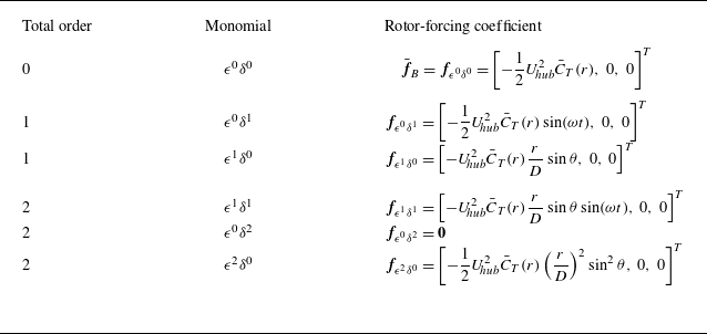

 u¯B
 (a)
 (b)

 (a)
 f^ϵ0δ1,x
 (b)
 f^ϵ1δ1,x
 U hub2

 ϵ=0.1
 St

 St=0.25
 y=0
 ϵ=0.1,δ=0.04
 a,b
 ϵ0δ1u^ϵ0δ1
 c,d
 ϵ1δ0uϵ1δ0
 e,f
 ϵ1δ1u^ϵ1δ1
 g,h

 ϵ1δ1
 (a,b)
 (c,d)

 xOy
 ϵ=0.1
 St=0.25
 a
 u^x
 b
 u^y

 St=0.25
 xOz
 ϵ
 a,b
 ϵ=0
 c,d
 ϵ=0.1
 e,f
 ϵ=0.2
 u^x
 u^z

 x=8D
 St
 ϵ

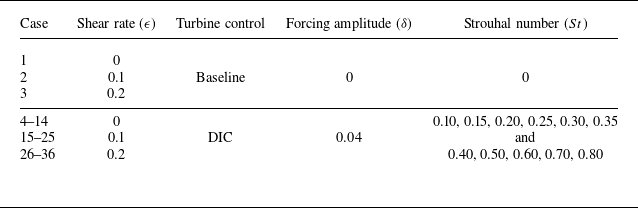

 ϵ
 α
 z0
 z hub
 D

 Δux/U hub
 y=0
 ϵ=0.0,0.1,0.2
 St=0.10,0.25,0.50

 σzc(x)/D
 a
 b
 d
 St=0.10
 0.25
 0.50
 ϵ

 u^z/U hub
 y=0
 ϵ=0.0,0.1,0.2
 St=0.10,0.25,0.50

 u^x/U hub

 u^y/U hub

 u^x/U hub

 Δu¯x/U hub
 y=0
 ϵ
 St

 ΔU~x/U hub
 r⩽0.5D
 a
 b−d
 St=0.10
 0.25
 0.50
 ϵ

 W1/2(x)/D
 y=0
 a
 b
 d
 St=0.10
 0.25
 0.50
 ϵ=0,0.1,0.2
 ϵ

 τxz/U hub2
 y=0
 ϵ
 St

 τ~xz=−⟨ux′uz′¯⟩y
 ⟨⋅⟩y=(1/D)∫−D/2D/2(⋅)dy
 z=±0.5D
 (a)
 (b)
 St=0.25
 τ~xz>0
 τ~xz<0
 ϵ

 St=0.25
 (a−c)
 St=0.25
 (d−f)
 ϵ=0
 (a,d)
 ϵ=0.1
 (b,e)
 ϵ=0.2
 (c,f)
 MC
 PT
 TC
 DF
 TP
 DP

 x=8D
 St
 ϵ

 u^z/U hub
 (a)
 (b)
 (c)
 u^z/U hub
 (d)
 z=−0.5D
 (e)
 z=0
 (f)
 z=0.5D
 St=0.25
 ϵ=0.1

 u^z
 a−c
 d−f
 g−i
 ϵ=0
 a,d,g
 ϵ=0.1
 b,e,h
 ϵ=0.2
 c,f,i
 St=0.25


 u^z
 a−c
 d−f
 g−i
 St=0.10
 a,d,g
 St=0.25
 b,e,h
 St=0.50
 c,f,i
 ϵ=0.1


 (a−c)
 (d−f)
 St=0.25
 δ=0.04
 (g−i)
 St=0.25
 δ=0.08
 T1=2.5%
 (a,d,g)
 T2=5.0%
 (b,e,h)
 T3=7.5%
 (c,f,i)
 ϵ=0.2

 St=0.25
 δ=0.04
 δ=0.08
 ϵ=0.2


