2.1 Non-homgeneous triangle map

Fix the simplex

$$ \begin{align*}\triangle = \{ (x_1, \ldots, x_n) \in {\mathbb R}^n:1\geq x_1 \cdots \geq x_n\geq 0\}.\end{align*} $$

Partition this simplex into sub-simplices

$$ \begin{align*}\triangle_b = \{ \mathbf{x}\in \triangle: 1-x_1 -bx_n \geq 0>1-x_1- (b+1) x_n \}. \end{align*} $$

Here,

$$ \begin{align*}b=\bigg\lfloor \frac{1-x_1}{x_n} \bigg\rfloor.\end{align*} $$

Definition 2.1. The triangle map

$$ \begin{align*}T:\triangle \rightarrow \triangle\end{align*} $$

is defined as

$$ \begin{align*}T(x_1, \ldots, x_n) = \bigg(\frac{x_2}{x_1}, \ldots , \frac{x_n}{x_1}, \frac{1-x_1-b x_n}{x_1}\bigg)\end{align*} $$

for any $(x_1, \ldots , x_n) \in \triangle _b.$

When $n=1$ , this is the classical Gauss map.

Definition 2.2. The triangle sequence for any $\mathbf {x}\in \triangle $ is a sequence

$$ \begin{align*}(b_0,b_1, \ldots)\end{align*} $$

of non-negative integers such that

$$ \begin{align*}\mathbf{x }\in \triangle_{b_0}, T(\mathbf{x}) \in \triangle_{b_1}, T^{(2)}(\mathbf{x}) \in \triangle_{b_2}, \ldots .\end{align*} $$

For any $x\in [0,1]$ , its triangle sequence encodes the classical continued fraction expansion of x.

In turn, this suggests the following definition.

Definition 2.3. For any sequence of non-negative integers

$$ \begin{align*}(b_0,b_1, \ldots),\end{align*} $$

the corresponding cylinder is

$$ \begin{align*}\triangle (b_0, \ldots, b_k)= \{\mathbf{x } \in \triangle_{b_0}: T(\mathbf{x}) \in \triangle_{b_1}, T^{(2)}(\mathbf{x}) \in \triangle_{b_2}, \ldots, T^{(k)}(\mathbf{x}) \in \triangle_{b_k}\}.\end{align*} $$

2.2 Homogeneous triangle map

Here, we start with the cone

$$ \begin{align*}\triangle^H = \{(x_0, x_1, \ldots, x_n)\in {\mathbb R}^{n+1} : x_0>x_1 > \cdots > x_n>0\}.\end{align*} $$

The superscript H stands for ‘homogeneous’. We partition this cone into sub-cones

$$ \begin{align*}\triangle_b^H = \{ \mathbf{x}\in \triangle: x_0-x_1 -bx_n \geq 0>x_0-x_1- (b+1) x_n \}. \end{align*} $$

Then, we have the following definition.

Definition 2.4. The (homogeneous) triangle map

$$ \begin{align*}T:\triangle^H \rightarrow \triangle^H\end{align*} $$

is defined as

$$ \begin{align*}T(x_0, \ldots, x_n) =(x_1, x_2, \ldots, x_n, x_0 - x_1 - bx_n)\end{align*} $$

for any $(x_0, \ldots , x_n) \in \triangle _b^H.$

When we need to distinguish this map T from the T in §2.1, we will use $T^H$ .

If we write each $\mathbf {x}=(x_0, \ldots , x_n) $ as a column vector, we can describe the map T via matrix multiplication:

$$ \begin{align*} T(\mathbf{x} ) &= T_b\left( \begin{array}{c} x_0 \\ \vdots \\ x_n \end{array} \right) \quad\mbox{if } \mathbf{x} \in \triangle_b^H\\ &= \left( \begin{array}{cccccc} 0&1&0&\cdots &0 &0 \\ 0&0&1& \cdots &0&0 \\ & & \vdots & & & \\ 0&0&0& \cdots &0& 1 \\ 1 & -1 & 0 &\cdots &0& -b \end{array} \right) \left( \begin{array}{c} x_0 \\ \vdots \\ x_n \end{array} \right) \quad\mbox{if } \mathbf{x} \in \triangle_b^H\\ &= \left( \begin{array}{c} x_1 \\ x_2 \\ \vdots \\ x_n \\ x_0-x_1-bx_n \end{array} \right). \end{align*} $$

The link between the homogeneous and the non-homogeneous triangle maps is the following. We have a projection

$$ \begin{align*}P:\triangle^H \rightarrow \triangle\end{align*} $$

given by

$$ \begin{align*}P(x_0, \ldots , x_n) =\bigg( \frac{x_1}{x_0}, \ldots, \frac{x_n}{x_0} \bigg).\end{align*} $$

It is straightforward to show that 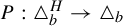$P:\triangle _b^H \rightarrow \triangle _b$ is onto. What is key is that the following diagram is commutative:

We have the embedding

$$ \begin{align*}i:\triangle \rightarrow \triangle^H\end{align*} $$

given by

$$ \begin{align*}i(x_1, \ldots, x_n) =( 1, x_1, x_2, \ldots, x_n).\end{align*} $$

This allows us to translate calculations for the non-homogeneous triangle map into calculations for the homogeneous triangle map, which in turn allows us to use simple linear algebraic tools.

Finally, we have the following definition.

Definition 2.5. The triangle sequence for any $\mathbf {x}\in \triangle ^H$ is a sequence

$$ \begin{align*}(b_0,b_1, \ldots)\end{align*} $$

of non-negative integers such that

$$ \begin{align*}\mathbf{x }\in \triangle_{b_0}, T(\mathbf{x}) \in \triangle_{b_1}, T^{(2)}(\mathbf{x}) \in \triangle_{b_2}, \ldots .\end{align*} $$

Definition 2.6. For any sequence of non-negative integers

$$ \begin{align*}(b_0,b_1, \ldots),\end{align*} $$

the corresponding cylinder is

$$ \begin{align*}\triangle^H (b_0, \ldots, b_k)= \{\mathbf{x } \in \triangle_{b_0}^H: T(\mathbf{x}) \in \triangle_{b_1}^H, T^{(2)}(\mathbf{x}) \in \triangle_{b_2}^H, \ldots, T^{(k)}(\mathbf{x}) \in \triangle_{b_k}^H\}.\end{align*} $$

2.3 The sliced non-homogeneous triangle map

(While all of this is standard, our nomenclature of using the term ‘slice’ is not.) For any vector $\mathbf {x} = (x_0, x_1, \ldots , x_n)$ , denote its $\ell _1$ norm as

$$ \begin{align*}\|\mathbf{x } \| = |x_0| + \cdots + |x_n|.\end{align*} $$

Set

$$ \begin{align*}\triangle^S = \{ \mathbf{x }\in \triangle^H : \|\mathbf{x}\|=1\} .\end{align*} $$

(We are using the superscript ‘S’ for slice, as $\triangle ^S = \triangle ^H \cap \{\|\mathbf {x}\| = 1\}$ .) This is an n-dimensional simplex. We have the natural projection

$$ \begin{align*}P^S:\triangle^H \rightarrow \triangle^S\end{align*} $$

given by

$$ \begin{align*}P^S(\mathbf{x}) = \frac{\mathbf{x}}{ \|\mathbf{x}\|}.\end{align*} $$

We set

$$ \begin{align*}\triangle_b^S= \triangle^S \cap \triangle_b^H.\end{align*} $$

Definition 2.7. The sliced non-homogeneous triangle map

$$ \begin{align*}T:\triangle^S \rightarrow \triangle^S\end{align*} $$

is

$$ \begin{align*}T(\mathbf{x}) = \frac{T^H(\mathbf{x})}{\|T^H(\mathbf{x})\|},\end{align*} $$

where the map $T^H$ on the right-hand side is the homogeneous triangle map.

When we need to distinguish this map T from the T in the previous §2.1 or from $T^H$ , we will use $T^S$ .

Definition 2.8. The triangle sequence for any $\mathbf {x}\in \triangle ^S$ is a sequence

$$ \begin{align*}(b_0,b_1, \ldots)\end{align*} $$

of non-negative integers such that

$$ \begin{align*}\mathbf{x }\in \triangle_{b_0}^S, T(\mathbf{x}) \in \triangle_{b_1}^S, T^{(2)}(\mathbf{x}) \in \triangle_{b_2}^S, \ldots .\end{align*} $$

The composition of

$$ \begin{align*} P^S\circ i:\triangle \rightarrow \triangle^S\end{align*} $$

gives us

$$ \begin{align*} (x_1,x_2 \ldots) & \xrightarrow{i} (1, x_1, x_2, \ldots)\\ &\xrightarrow{P^S} \bigg( \frac{1}{1+x_1+ \cdots + x_n},\frac{x_1}{1+x_1+ \cdots + x_n}, \ldots, \frac{x_n}{1+x_1+ \cdots + x_n} \bigg). \end{align*} $$

Definition 2.9. For any sequence of non-negative integers

$$ \begin{align*}(b_0,b_1, \ldots),\end{align*} $$

the corresponding cylinder is

$$ \begin{align*}\triangle^S (b_0, \ldots, b_k)= \{\mathbf{x } \in \triangle_{b_0}^S: T(\mathbf{x}) \in \triangle_{b_1}^S, T^{(2)}(\mathbf{x}) \in \triangle_{b_2}^S, \ldots, T^{(k)}(\mathbf{x}) \in \triangle_{b_k}^S\}.\end{align*} $$

We have the following lemma.

Lemma 2.10. For all non-negative integers $b_0, b_1, b_2$ , the map

$$ \begin{align*}\triangle(b_0, b_1, \ldots, b_k) \xrightarrow{P^S\circ i}\triangle(b_0, b_1, \ldots, b_k) \end{align*} $$

is a continuous, one-to-one, onto map.

3.1 Definition of weak convergence

Definition 3.1. Let $\mathbf {x} \in \triangle $ have triangle sequence $(b_0, b_1, \ldots ).$ We say the the triangle map weakly converges to $\mathbf {x}$ if

$$ \begin{align*}\lim_{m\rightarrow \infty} \bigcap_{k=0}^m \triangle(b_0, \ldots, b_m) = \{\mathbf{x}\}.\end{align*} $$

By Lemma 2.10, we have that the triangle map will weakly converge to $\mathbf {x} \in \triangle $ precisely when

$$ \begin{align*}\lim_{m\rightarrow \infty} \bigcap_{k=0}^m \triangle^S(b_0, \ldots, b_m) = \{P^S\circ(\mathbf{x})\}.\end{align*} $$

We will be doing most of our work on convergence in the world of $\triangle ^S$ and $\triangle ^H.$

In the $n=1$ and hence the classical continued fraction case, there is weak convergence for all $\mathbf {x}.$ As discussed in [Reference Assaf, Chen, Cheslack-Postava, Cooper, Diesl, Garrity, Lepinski and Schuyler2, Reference Garrity13, Reference Messaoudi, Nogueira and Schweiger22], this is not the case for $n=2$ , when the limit $\lim _{m\rightarrow \infty } \bigcap _{k=0}^m \triangle (b_0, \ldots , b_m) $ can be an entire line segment. However, the key technical part of the work of Messaoudi, Nogueira, and Schweiger was their Theorem 1.1, where they show that weak convergence does happen if infinitely many of the $b_k$ we have $b_k=0$ . Coupled with their Theorem 1.2, which states that almost every point $\mathbf {x}\in \triangle $ , with respect to Lebesgue measure, has infinitely many of their $b_k=0$ , allows them to prove ergodicity in the $n=2$ case.

For higher dimensions, the convergence of $\lim _{m\rightarrow \infty } \bigcap _{k=0}^m \triangle (b_0, \ldots , b_m) $ appears that it can be any simplex up to dimension $n-1$ . Further, just requiring infinitely many of the $b_k=0$ is no longer a strong enough condition to guarantee weak convergence.

One of our main technical goals is the following theorem.

This theorem will follow from our true technical goal, which will take some work.

In Corollary 4.2, we will show that this happens almost everywhere with respect to Lebesgue measure, which in turn will allow us to finally prove ergodicity.

3.2 Vertices of the subcells

This part is, relatively speaking, a straightforward generalization of [Reference Assaf, Chen, Cheslack-Postava, Cooper, Diesl, Garrity, Lepinski and Schuyler2, §4] and of the introduction of [Reference Messaoudi, Nogueira and Schweiger22].

Fix a sequence $(b_0, b_1, \ldots )$ of non-negative integers. Denote the vertices of $\triangle ^H(b_0, \ldots , b_m)$ as

$$ \begin{align*}A_0(m), \ldots, A_n(m).\end{align*} $$

Then, the vertices of $\triangle ^S(b_0, \ldots , b_m)$ are

$$ \begin{align*} \frac{A_0(m)}{\|A_0(m) \|}, \ldots, \frac{A_n(m)}{\|A_n(m) \|}.\end{align*} $$

The goal of Theorem 3.2 is now equivalent to showing that the distances between the vertices of $\triangle ^S(b_0, \ldots , b_m)$ approach zero.

Lemma 3.4. For a sequence $(b_0, b_1, \ldots )$ of non-negative integers, we have that $\lim _{m\rightarrow \infty } \bigcap _{k=0}^m \triangle ^S(b_0, \ldots , b_m) $ is a single point if and only if, for all i and j,

$$ \begin{align*}\lim_{m\rightarrow \infty} \bigg| \frac{A_i(m)}{\|A_i(m) \|} - \frac{A_j(m)}{\|A_j(m) \|},\bigg|_2 =0.\end{align*} $$

Building on work in [Reference Assaf, Chen, Cheslack-Postava, Cooper, Diesl, Garrity, Lepinski and Schuyler2, Reference Messaoudi, Nogueira and Schweiger22], we can recursively define the vertices of each $\triangle ^H(b_0, \ldots , b_m)$ . We have the following lemma.

Lemma 3.5. We have

$$ \begin{align*}A_i(m+1)&=A_{i+1}(m) \quad \text{for }i\in \{0, 2, \ldots, n-2\},\\A_{n-1}(m+1)&=b_{m+1}A_0(m)+A_n(m),\\A_{n}(m+1) &= (b_{m+1}+1)A_0(m) +A_n(m). \end{align*} $$

For the dimension n case, the vertices of each $\triangle ^H(b_0, \ldots , b_m)$ are vectors in ${\mathbb R}^{n+1}$ . The initial simplex $\triangle ^H$ has vertices

$$ \begin{align*}A_0 = \left( \begin{array}{c} 1 \\ 0 \\ \vdots \\ 0 \end{array} \right), A_1 = \left( \begin{array}{c} 1 \\ 1\\0 \\ \vdots \\ 0 \end{array} \right), \ldots, A_n = \left( \begin{array}{c} 1 \\ 1 \\ \vdots \\ 1 \end{array} \right)\end{align*} $$

giving us that the vertices of $\triangle ^H(b_0)$ are

$$ \begin{align*}A_0(0) = \left( \begin{array}{c} 1 \\ 1 \\ 0 \\ \vdots \\ 0 \end{array} \right), A_1(0) = \left( \begin{array}{c} 1 \\ 1\\1\\ 0 \\ \vdots \\ 0 \end{array} \right), \ldots, A_{n-2}(0) = \left( \begin{array}{c} 1 \\ \vdots \\ 1 \\ 0 \end{array}\right),\end{align*} $$

$$ \begin{align*}A_{n-1}(0) = \left( \begin{array}{c} b_0 +1 \\ 1 \\ \vdots \\ 1 \end{array} \right), A_n(0) = \left( \begin{array}{c} b_0+2 \\ 1 \\ \vdots \\ 1 \end{array} \right).\end{align*} $$

As a schematic diagram, we can think of this as follows.

Let $m>n.$ Suppose that there is a constant B such that

$$ \begin{align*}b_{m-(n-2)}, b_{m-(n-3)}, \ldots, b_m \leq B.\end{align*} $$

For notational convenience, set

$$ \begin{align*}b_{m-(n-1)}=b,\end{align*} $$

where b could be any non-negative integer. Finally, again for notational convenience, denote

$$ \begin{align*}A_i(m-n) = A_i.\end{align*} $$

Then, we have the following lemma.

Lemma 3.6. We have

$$ \begin{align*} A_0(m) &= bA_0 + A_n, \\A_1(m) &= b_{m-(n-2)}A_1 + (b+1) A_0 + A_ n, \\A_2(m) &= b_{m-(n-3)} A_2 + (b_{m-(n-2)}+1) A_1 + (b+1) A_0 + A_ n,\\A_3(m) &= b_{m-(n-4)} A_3 + (b_{m-(n-3)} +1) A_2 + (b_{m-(n-2)}+1) A_1 + (b+1) A_0 + A_ n, \\&\ \ \vdots \\A_{n-2}(m ) &= b_{m-1} A_{n-2} + (b_{m-2}+1) A_{n-3} + \cdots + (b_{m-(n-2)}+1) A_1 + (b+1) A_0 + A_ n , \\A_{n-1}(m) &= b_mA_{n-1} +(b_{m-1}+1) A_{n-2} + (b_{m-2}+1) A_{n-3} \\& \quad + \cdots + (b_{m-(n-2)}+1) A_1 + (b+1) A_0 + A_ n , \\A_n(m ) &= (b_m+ 1) A_{n-1} +(b_{m-1}+1) A_{n-2} + (b_{m-2}+1) A_{n-3} \\& \quad + \cdots + (b_{m-(n-2)}+1) A_1 + (b+1) A_0 + A_ n. \end{align*} $$

3.3 Control of growth of vertices

We need to understand how the vertices $A_i(m)$ grow in their $\ell _1$ norm. From the recursive formula and from the fact that all of the $b_i$ are non-negative, we have the following lemma.

Lemma 3.7. For all m, we have

$$ \begin{align*}\|A_0(m) \| < \| A_1(m)\| < \cdots < \|A_n(m)\|\end{align*} $$

and for all i,

$$ \begin{align*}\|A_i(m) \| \leq \|A_i(m+1)\|.\end{align*} $$

However, we also have that the ratios of the

$$ \begin{align*}\|A_k(m)\|\end{align*} $$

cannot grow too quickly, under assumptions of control on the size of the various $b_k.$

Lemma 3.8. Let $m>n.$ Suppose that there is a constant B such that

$$ \begin{align*}b_{m-(n-2)}, b_{m-(n-3)}, \ldots, b_m \leq B.\end{align*} $$

Then, for all $i<j$ , we have

$$ \begin{align*}\frac{ \|A_i(m)\|}{\|A_j(m)\|}\geq \frac{1}{(B+1)(n+1)}.\end{align*} $$

Proof. We have

$$ \begin{align*} \frac{ \|A_i(m)\|}{\|A_j(m)\|}&\geq \frac{ \|A_0(m)\|}{\|A_n(m)\|}\\&= \frac{ \|bA_0 + A_n\|}{\|(b_m+ 1) A_{n-1} + \cdots + (b_{m-(n-2)}+1) A_1 + (b+1) A_0 + A_ n \| }\\& \qquad \text{using Lemma 3.6 and its notation}\\&\geq \frac{ \|bA_0 + A_n\|}{\|(B+ 1) (bA_0 + A_n) + \cdots + (B+1) (bA_0 + A_n) + bA_0 + A_ n \| }\\&\geq \frac{1}{(B+1)(n+1)}.\\[-41pt] \end{align*} $$

3.4 Weak convergence: proof of Theorem 3.2

We need a little more notation. Given two non-zero vectors U and V in ${\mathbb R}^n_{\ge 0}$ , define a distance function

$$ \begin{align*}D(U,V):=\bigg|\frac{U}{\|U\|}-\frac{V}{\|V\|} \bigg|_2.\end{align*} $$

We have

(3.1) $$ \begin{align} D(U, U+V)=\bigg|\frac{U}{\|U\|}-\frac{V}{\|U+V\|} \bigg|_2=\frac{\|V\|}{\|U+V\|}D(U,V), \end{align} $$

which is straightforward, with a lower dimensional case originally proven in [Reference Messaoudi, Nogueira and Schweiger22].

Set

$$ \begin{align*}d(k) = \max_{i,j} D(A_i(k), A_j(k)).\end{align*} $$

Then, $d(k)$ is the diameter of the simplex

$$ \begin{align*}\triangle^S(b_0, \ldots, b_k).\end{align*} $$

We have

$$ \begin{align*}d(0)\geq d(1) \geq d(2) \geq \cdots.\end{align*} $$

We will have weak convergence precisely when

$$ \begin{align*}\lim_{k\rightarrow \infty}d(k) = 0.\end{align*} $$

Let $m>n$ and assume that there is a constant B such that

$$ \begin{align*}b_{m-(n-2)}, b_{m-(n-3)}, \ldots, b_m \leq B.\end{align*} $$

We will show that

$$ \begin{align*}d(m) \leq \frac{Bn + B + n}{Bn + B + n + 1} d(m-n).\end{align*} $$

As there are infinitely many such m with corresponding bounds $b_{m-(n-2)}, b_{m-(n-3)}, \ldots , b_m \leq B,$ we will have our limit.

One last point, before setting up the needed string of inequalities. For all $j>i$ , using Lemma 3.6, we know that both $A_i(m)$ and $A_j(m) - A_i(m)$ are in the simplex $\triangle ^H(b_0, \ldots , b_{m-n})$ , which gives us

$$ \begin{align*}D(A_i(m), A_j(m) - A_i(m))\leq d(m-n).\end{align*} $$

For $i<j$ , we have

$$ \begin{align*} D(A_i(m), A_j(m) )&= D(A_i(m), A_i+ (A_j(m)-A_i(m) ))\\ &= \frac{\|A_j(m)-A_i(m)\|}{\|A_j(m)\|}D(A_i(m),A_j(m)-A_i(m))\\ &\leq \frac{\|A_j(m)-A_i(m)\|}{\|A_j(m)\|}d(m-n)\\ &= \bigg( 1 - \frac{\|A_i(m)\|}{\|A_j(m)\|}\bigg) d(m-n)\\ &\leq \bigg( 1 - \frac{1}{(B+1)(n+1)}\bigg) d(m-n)\\ &= \frac{Bn + B + n}{Bn + B + n + 1} d(m-n). \end{align*} $$

Theorem 3.2 is true.

4.1 Key theorem on convergence almost everywhere

This section contains the needed preliminaries for §6, where we will finally show that the triangle map is ergodic.

Here, we show the following theorem.

We will actually prove a subset of the above also happens almost everywhere.

This will give us the following corollary.

Proving Theorem 4.2 will take work and is the most technical part of this paper.

4.2 Key proposition for weak convergence almost everywhere

We will throughout assume that $m>n$ , where n is the dimension of the triangle map.

Proposition 4.4. Let $b_0, \ldots , b_{m-n}$ be any sequence of non-negative integers. Let

$$ \begin{align*}R = \bigcup_{b_i>0} \triangle^S(b_0, \ldots, b_{m-n},b,\underbrace{0,0,\ldots, 0}_{n-1 \ \mathrm{zeroes}}).\end{align*} $$

Then,

$$ \begin{align*}\frac{\unicode{x3bb}(R)}{\unicode{x3bb}(\triangle^S(b_0, \ldots, b_{m-n})}>\frac{1}{(n-1)(n)(n+1)\cdots(2n-2)n^{n-1}},\end{align*} $$

where $\unicode{x3bb} $ is Lebesgue measure.

The proof of this proposition will take some work, spread out over the next few subsections.

Let us first, though, see why this proposition will imply Theorem 4.2.

4.3 Preliminary lemma on volume

We will be using the notation as in §3.2. In particular, let $b_0, \ldots , b_{n-4}$ be any sequence of non-negative integers. Let $A_0, \ldots , A_n$ be the column vectors in ${\mathbb R}^{n+1}$ that define the cone $\triangle ^H(b_0, \ldots , b_{n-4})$ , as described earlier. Then,

$$ \begin{align*}\bigg\{\frac{A_0}{\|A_0 \| } , \ldots, \frac{A_n}{\|A_n \|}\bigg\}\end{align*} $$

are the vertices of the simplex $\triangle ^S(b_0, \ldots , b_{n-4})$ . We will need to use the following lemma (which is already known, though not quite in this language).

Lemma 4.5. We have

$$ \begin{align*}\unicode{x3bb}(\triangle^S(b_0, \ldots, b_{m-4}))=\frac{\sqrt{n}}{(n-1)!\|A_1\|\;\|A_2\|\cdots\|A_n\|}.\end{align*} $$

Let $b\in {\mathbb Z}_{\ge 1}$ . Then,

$$ \begin{align*}\unicode{x3bb}(\triangle^S(b_0, \ldots, b_{m-4},b,\underbrace{0,0,\ldots, 0}_{n-2 \ \mathrm{zeroes}}))\end{align*} $$

is

$$ \begin{align*}\frac{\sqrt{n}}{(n-1)!\|bA_1+A_n\|\;\|(b+1)A_1+A_n\|\;\|(b+1)A_1+A_2+A_n\|\cdots\|(b+1)A_1+A_2+\cdots+A_n\|}.\end{align*} $$

Proof. The first part of the lemma is proven in [Reference Messaoudi, Nogueira and Schweiger22, Lemma 3.2]. We simply have to consider the $(n+1) \times (n+1)$ matrix whose columns are $A_0, \ldots , A_n,$ and observe that this matrix is the product of the matrices of the form $T_{b_k}$ , as defined in §2.2, each of which has determinant $\pm 1.$

As seen in Lemma 3.6, the vertices of the cell $\triangle ^S(b_0, \ldots , b_{m-4},b,\underbrace {0,0,\ldots , 0}_{n-2 \text { zeroes}})$ are

$$ \begin{align*}A_1^n=bA_1+A_n, A_2^n=A_1^n+A_1, A_3^n=A_2^n+A_2, \ldots, A_n^n=A_{n-1}^n+A_{n-1}.\end{align*} $$

Thus, plugging in for these vertices, we have the result.

4.4 First combinatorial identity

Our goal is to show that points with $n-1$ zeroes in a row early in their triangle sequence occupy an appreciable proportion of each cell. Our proof of this requires a pair of strictly combinatorial lemmas, which we present in this subsection and in the next. In addition to their relevance to the ergodicity result, they are interesting in their own right.

Lemma 4.6. For any integers $0 \leq j \leq n,$ the following holds:

$$ \begin{align*}\sum_{j=0}^{n-2} \frac{{n-2\choose j}(-1)^j}{(j+1)x+y}=\frac{(n-2)!\cdot x^{n-2}}{(x+y)(2x+y)(3x+y)\cdots((n-1)x+y)}.\end{align*} $$

Example 4.7. (The $n = 4$ example)

Before proving this strange lemma, we give an explicit example of what it is claiming. Plugging in $n=4$ on the left-hand side, we get

$$ \begin{align*} &\frac{{2\choose0}(-1)^0}{x+y}+\frac{{2\choose1}(-1)^1}{2x+y}+\frac{{2\choose2}(-1)^2}{3x+y} \\ &\quad=\frac{1}{x+y}+\frac{-2}{2x+y}+\frac{1}{3x+y} \\ &\quad=\frac{2x+y-2(x+y)}{(x+y)(2x+y)}+\frac{1}{3x+y} \\ &\quad=\frac{-y}{(x+y)(2x+y)}+\frac{1}{3x+y} \\ &\quad=\frac{-y(3x+y)+(x+y)(2x+y)}{(x+y)(2x+y)(3x+y)} \\ &\quad=\frac{-3xy-y^2+2x^2+2xy+xy+y^2}{(x+y)(2x+y)(3x+y)} \\ &\quad=\frac{2x^2}{(x+y)(2x+y)(3x+y)}, \end{align*} $$

which matches the expression on the right-hand side of the lemma.

Proof. We prove this by induction, with thanks to L. Pedersen, who suggested the proof strategy. First, factor out the y from the denominators in the sum and perform the substitution $u=x/y$ to yield

(4.1) $$ \begin{align} &\sum_{j=0}^{n-2} \frac{(-1)^j{{n-2}\choose j}}{(j+1)x+y} \notag \\ &\quad= \frac{{{n-2}\choose {0}}}{x+y} - \frac{{{n-2}\choose {1}}}{2x+y}+\frac{{{n-2}\choose {2}}}{3x+y}-\cdots +(-1)^{n-2}\frac{{{n-2}\choose {n-2}}}{(n-1)x+y} \notag \\ &\quad= \frac{1}{y}\bigg[\frac{{{n-2}\choose {0}}}{1+u} - \frac{{{n-2}\choose {1}}}{1+2u}+\frac{{{n-2}\choose {2}}}{1+3u}-\cdots +(-1)^{n-2}\frac{{{n-2}\choose {n-2}}}{1+(n-1)u}\bigg]. \end{align} $$

We now study the bracketed expression. Note that when $n=3$ , the expression is ${1}/({1+u})-{1}/({1+2u})$ , which equals ${u}/{(1+u)(1+2u)}$ . For our inductive base case, we will need something slightly stronger, which is that this expression holds for any pair of consecutive positive integer multiples of u, not just u and $2u$ . Let r be the starting value. Our base case is

(4.2) $$ \begin{align} \frac{1}{1+ru}-\frac{1}{1+(r+1)u}=\frac{u}{(1+ru)(1+(r+1)u)}. \end{align} $$

Now suppose that for some positive integer $k\ge 3$ , we have that for any positive integer r,

(4.3) $$ \begin{align} \notag &\frac{{{k-2}\choose {0}}}{1+ru} - \frac{{{k-2}\choose {1}}}{1+(r+1)u}+\frac{{{k-2}\choose {2}}}{1+(r+2)u}-\cdots +(-1)^{k-2}\frac{{{k-2}\choose {k-2}}}{1+(r+k-2)u} \\&\quad= \frac{(k-2)!\cdot u^{k-2}}{(1+ru)(1+(r+1)u)\cdots(1+(r+k-2)u)}. \end{align} $$

Recall Pascal’s identity, namely ${n\choose {k-1}}+{n\choose {k}}={{n+1}\choose {k}}$ . Applying this down the columns in the following equation subtraction, we have that

$$ \begin{align*} &\frac{{{k-2}\choose {0}}}{1+ru} - \frac{{{k-2}\choose {1}}}{1+(r+1)u}+\frac{{{k-2}\choose {2}}}{1+(r+2)u}-\cdots +(-1)^{k-2}\frac{{{k-2}\choose {k-2}}}{1+(r+k-2)u}\\&\quad-\bigg[\frac{{{k-2}\choose {0}}}{1+(r+1)u} - \frac{{{k-2}\choose {1}}}{1+(r+2)u}+\cdots +(-1)^{k-3}\frac{{{k-2} \choose {k-3}}}{1+(r+k-2)u}\\&\quad+(-1)^{k-2}\frac{{{k-2}\choose {k-2}}}{1+(r+k-1)u}\bigg]\\[6pt]\hline \\[-6pt]&\frac{{{k-1}\choose {0}}}{1+ru} - \frac{{{k-1}\choose {1}}}{1+(r+1)u}+\frac{{{k-1}\choose {2}}}{1+(r+2)u}-\cdots+(-1)^{k-2}\frac{{{k-1}\choose {k-2}}}{1+(r+k-2)u}\\&\quad+(-1)^{k-1}\frac{{{k-2}\choose {k-2}}}{1+(r+k-1)u}. \end{align*} $$

(The above is a massive fraction. The part above the long horizontal line is the numerator while the part below the long horizontal line is the denominator.)

By equation (4.3), we know the first line in the subtraction equals ${(k-2)!\cdot u^{k-2}}/ (1+ru)(1+(r+1)u)\cdots (1+(r+k-2)u)$ and the second equals ${(k-2)!\cdot u^{k-2}}/ (1+(r+1)u)(1+(r+2)u)\cdots (1+(r+k-1)u)$ . Subtracting these yields

(4.4) $$ \begin{align} &\notag (k-2)!\cdot u^{k-2}\frac{(k-1)u}{(1+ru)(1+(r+1)u)\cdots(1+(r+k-1)u)} \\ &\quad=\frac{(k-1)!\cdot u^{k-1}}{(1+ru)(1+(r+1)u)\cdots(1+(r+k-1)u)}. \end{align} $$

Thus, if equation (4.3) holds for k, it holds for $k+1$ , so since we have the base case $k=3$ for all r, we know that equation (4.3) holds for any r and all $k \ge 3$ .

Taking $r=1$ and $k=n$ in equation (4.3), we can now substitute back into equation (4.1) to yield that our original summation equals

$$ \begin{align*} \frac{1}{y}\bigg[\frac{(n-2)!\cdot u^{n-2}}{(1+u)(1+2u)\cdots(1+(n-1)u)} \bigg]. \end{align*} $$

Now, substituting back in for $u=x/y$ , the $k-1$ factors of $1/y$ in the bracketed denominator cancel with the $k-2$ factors of $1/y$ in the numerator and the extra in front, leaving us with

$$ \begin{align*}\sum_{j=0}^{n-2} \frac{{{n-2}\choose j}(-1)^j}{(j+1)x+y}=\frac{(n-2)!\cdot x^{n-2}}{(x+y)(2x+y)(3x+y)\cdots((n-1)x+y)},\end{align*} $$

as desired.

4.5 Second combinatorial identity

The second of the combinatorial lemmas is more difficult to state, so we introduce it with the help of a diagram. The relevant coefficients will arise naturally in our ergodicity proof, but we can more easily envision deriving them as follows.

Recall that the multinomial $n \choose {k_1, k_2, \ldots , k_m}$ is defined as the way, given n items and m boxes total, to choose $k_i$ items to put into each box i. We are interested particularly in the case where every item is placed into a box, meaning 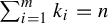$\sum _{i=1}^m k_i=n$ . Note that ${n \choose {k_1, k_2, \ldots , k_m}}={n!}/{k_1!k_2!\cdots k_m!}$ .

There are $2^{n-1}$ compositions of n. We define their standard order to be lexicographic order with higher numbers coming first. Thus, the standard order for compositions of 3 is $\{3\}, \{2,1\}, \{1,2\}, \{1,1,1\}$ .

Given the composition $\{k_1, k_2, \ldots , k_m\}$ , we naturally have a multinomial that corresponds, namely

$$ \begin{align*}{k_1+k_2+\cdots+k_m \choose k_1, k_2, \ldots, k_m}.\end{align*} $$

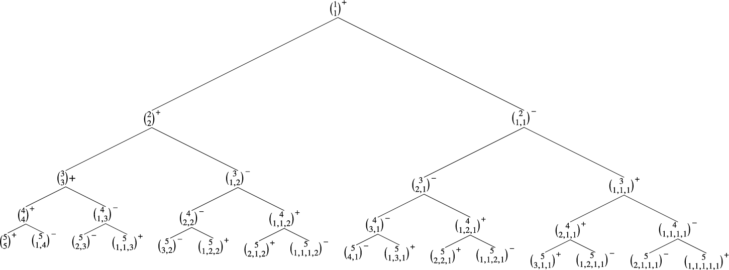
We can arrange all such multinomials into a binary tree as follows: let row n contain all multinomials corresponding to compositions of n. Beginning with $1\choose 1$ at the top, every node $n\choose {k_1, k_2, \ldots , k_m}$ has left child

$$ \begin{align*}{n+1\choose k_1+1, k_2, \ldots, k_m}\end{align*} $$

and right child

$$ \begin{align*}{n+1\choose 1, k_1, k_2, \ldots, k_m }.\end{align*} $$

We will now assign signs to the tree entries as follows: assign to $1\choose 1$ a $+$ and then, as we move down the tree, sign each left child the same as its parent and each right child the opposite. Note that since left children have the same number of composition parts as their parents and right children have one more, this rule is the same as signing $n\choose {k_1, k_2, \ldots , k_m}$ by $(-1)^{m-1}$ . See Figure 1 for the first five rows of the tree with the signs corresponding to each entry labeled. Now the following strange property emerges, which we will first state in terms of the tree, then more formally with reference only to the standard order. For any $0\le k \le n$ , the sum of the first $2^{k}$ signed entries in row $n+1$ equals $(-1)^{k}{n \choose k}$ .

Figure 1

First five rows of multinomial tree.

As an example, take $k=3$ and $n=4$ , which means we are looking at the sum of the first eight signed entries in row 5. These are $1-5-10+20-10+30+30-60=-4$ , which is ${4\choose 3}(-1)^3$ , as predicted.

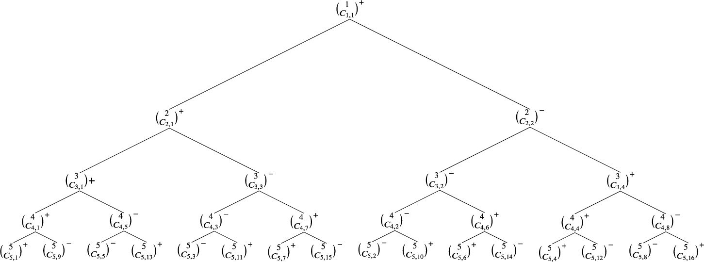
Let $C_{n,i}$ be the ith composition in standard order of the positive integer n and $|C_{n,i}|$ be the number of parts in $C_{n,i}$ . Thus, for example, $C_{5, 7}=\{2,1,2\}$ and $|C_{5, 7}|=3$ . Finally, let $n \choose C_{n,i}$ be the value of the multinomial corresponding to the composition $C_{n,i}$ , so ${5 \choose C_{5,7}}={5\choose {2,1,2}}={5!}/{2!1!2!}=30$ .

For clarity, Figure 2 shows the same tree from Figure 1, just rewritten with the new notation.

Figure 2

First five rows of multinomial tree with new notation.

We can now state the lemma without reference to the tree.

Lemma 4.9. For $n, k \in {\mathbb Z}_{\ge 0}$ with $k \le n$ ,

Proof. We prove the lemma by induction, returning to the tree for intuition. Let $S_n$ be the sum of the multinomials corresponding to compositions of n with their signs as listed in the tree. Equivalently,

$$ \begin{align*}S_n:=\sum_{i=1}^{2^{n-1}} {n \choose C_{n,i}}(-1)^{|C_{n,i}|-1}.\end{align*} $$

As a base case, note that 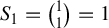$S_1 = {1 \choose 1}=1$ . Now suppose that for some $r \ge 0$ , the lemma holds for row $r+1$ of the tree as well as all rows above it, meaning for any $0 \le k \le n \le r$ , we have

The key thing to note is that every time we move right down the tree, we fix the last composition part size for all descendants of that node. Thus, the entire right half of the tree consists of multinomials corresponding to compositions ending in 1, the second quarter of the tree from the left consists of multinomials corresponding to compositions ending in 2, and in general the second ${1}/{2^j}$ th of the tree from the left consists of multinomials corresponding to compositions ending in j. Thus, in row $r+1$ , where we have $2^{r}$ entries in the tree, we see that reading them from left to right, we encounter first one multinomial corresponding to a composition ending in $r+1$ (the odd one out in a sense, since it is not the second unit in any binary division), then one multinomial corresponding to a composition ending in r, then two multinomials corresponding to a composition ending in $r-1$ , and so on, with $2^{j}$ compositions corresponding to multinomials ending in $r-j$ . These compositions correspond to the ways to place $j+1$ items into boxes, since we have $r+1$ items total, but are committing to having $r-j$ of them in our last box. Since there are only $2^j$ compositions of $j+1$ , their corresponding multinomials must all appear in row $r+1$ , each with a final part of size $r+1-(j+1)=r-j$ tacked on. In fact, our tree rules are such that those multinomials appear in the same order in row $r+1$ that they did originally in row $j+1$ , just each with the extra part added to make the components sum to $r+1$ . Thus, reading the compositions from each multinomial across the tree at row $r+1$ , we get first the entry ${r+1}$ , then what is essentially a copy of row 1, just with an r tacked on, then a copy of row 2 with an $r-1$ tacked on to each entry, then a copy of row 3 with an $r-2$ tacked on to each entry, and so on.

Since we are adding an entry to each composition, all the signs swap from how they appear in row $j+1$ to how they appear in row $r+1$ . The effects of replacing the sum from row $j+1$ with the copy of row $j+1$ that appears in row $r+1$ are as follows: first, the multinomial now has us picking from $r+1$ items instead of $j+1$ items, so the $(j+1)!$ in the numerator of the value in row $j+1$ is replaced by an $(r+1)!$ , for a net effect of multiplying by ${(r+1)!}/{(j+1)!}$ . Second, the tacked on $r-j$ contributes an $(r-j)!$ to the denominator of the version of the multinomial that appears in row $r+1$ . And third, as noted, the signs all swap from row $j+1$ to the copy of row $j+1$ embedded in row $r+1$ . Thus, the overall effect is that reading from left to right along row $r+1$ , we have that the entries from number $2^{j-1}+1$ to number $2^{j}$ sum to $-S_j({(r+1)!}/{(j+1)!})({1}/{(r-j)!})$ , or equivalently, to $-S_j\binom {r+1}{j+1}$ . Since $j < r+1$ , we have by our inductive assumption that 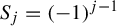$S_j=(-1)^{j-1}$ . We now have that the sums of chunks of increasing size reading along row $r+1$ are as follows:

• • the first entry, which is $\binom {r+1}{r+1}=1$ ;

• • the second entry, which is $-S_1\binom {r+1}{1}$ ;

• • the third and fourth entries, which sum to $-S_2\binom {r+1}{2}$ ;

• • entries 5–8, which sum to $-S_3\binom {r+1}{3}$ ;

• • and so on, with entries $2^{j-1}+1$ to $2^{j}$ summing to $-S_j\binom {r+1}{j}$ .

Now, we plug in for $S_n=(-1)^{n-1}$ and add up the items above. Writing the initial 1 as $\binom {r}{0}$ , we have that by Pascal’s identity, the sum of the first two entries in row $r+1$ is $\binom {r}{0}-\binom {r+1}{1}=-\binom {r}{1}$ . Then, the sum of the first four entries is $-\binom {r}{1}+\binom {r+1}{2}=\binom {r}{2}$ . Continuing, we see that the sum of the first $2^j$ entries in row $r+1$ is $\binom {r}{j}(-1)^j$ . Taking $j=r$ , we get that the sum of the entire row, $S_{r+1}$ , is equal to $\binom {r}{r}(-1)^{r}=(-1)^r$ , allowing us to use this in the simplification for future rows, as desired. This completes the proof of the lemma.

4.6 A lower bound

To prove the key Proposition 4.4 for weak convergence, we will need the following lemma.

Lemma 4.10. Using the notation of Proposition 4.4, we have

$$ \begin{align*}\sum_{b=1}^\infty \unicode{x3bb}\bigg(\bigcup_{b>0} \triangle^S(b_0, \ldots, b_{m-n},b,\underbrace{0,0,\ldots, 0}_{n-1 \ \mathrm{zeroes}})\bigg)\end{align*} $$

is strictly greater than

$$ \begin{align*} \frac{\sqrt n}{(n-1)!(n-1)\|A_0\|}\bigg(\frac{1}{\|A_0+A\|\;\|2A_0+A\|\cdots\|(n-1)A_0+A\|}\bigg),\end{align*} $$

where $A:=A_1+A_2+\cdots +A_n.$

Before we prove this lemma, we give an example for the $n=5$ case that illustrates the strategy. Then we have

$$ \begin{align*} &\frac{1}{\|bA_0+A_5\|\;\|(b+1)A_0+A_5\|\;\|(b+1)A_0+A_1+A_5\|\cdots\|(b+1)A_0+A_1+\cdots+A_5\|} \\ &\quad> \frac{1}{\|bA_0+A\|\;\|(b+1)A_0+A\|\;\|(b+2)A_0+A\|\cdots\|(b+4)A_0+A\|} \\ &\quad= \frac{1}{\|A_0\|}\bigg(\frac{1}{\|bA_0+A\|}-\frac{1}{\|(b+1)A_0+A\|}\bigg)\\ &\qquad\times\frac{1}{\|(b+2)A_0+A\|\;\|(b+3)A_0+A\|\;\|(b+4)A_0+A\|}\\ &\quad=\frac{1}{\|A_0\|}\bigg[\frac{1}{2\|A_0\|}\bigg(\frac{1}{\|bA_0+A\|}-\frac{1}{\|(b+2)A_0+A\|}\bigg) -\frac{1}{\|A_0\|} \bigg(\frac{1}{\|(b+1)A_0+A\|} \\ &\qquad-\frac{1}{\|(b+2)A_0+A\|}\bigg)\bigg] \cdot \frac{1}{\|(b+3)A_0+A\|\;\|(b+4)A_0+A\|}\\ &\quad=\frac{1}{\|A_0\|}\bigg[\frac{1}{2\|A_0\|}\bigg(\frac{1}{3\|A_0\|}\bigg(\frac{1}{\|bA_0+A\|}-\frac{1}{\|(b+3)A_0+A\|}\bigg)-\frac{1}{\|A_0\|}\bigg(\frac{1}{\|(b+2)A_0+A\|} \\ &\qquad-\frac{1}{\|(b+3)A_0+A\|}\bigg)\bigg)-\frac{1}{\|A_0\|}\bigg(\frac{1}{2\|A_0\|}\bigg(\frac{1}{\|(b+1)A_0+A\|}-\frac{1}{\|(b+3)A_0+A\|}\bigg) \\ &\qquad-\frac{1}{\|A_0\|}\bigg(\frac{1}{\|(b+2)A_0+A\|}-\frac{1}{\|(b+3)A_0+A\|}\bigg)\bigg)\bigg]\cdot \frac{1}{\|(b+4)A_0+A\|}\\ &\quad= \frac{1}{\|A_0\|}\bigg[\frac{1}{2\|A_0\|}\bigg(\frac{1}{3\|A_0\|}\bigg[\frac{1}{4\|A_0\|}\bigg(\frac{1}{\|bA_0+A\|}-\ast \bigg)-\frac{1}{\|A_0\|}\bigg(\frac{1}{\|(b+3)A_0+A\|}-\ast \bigg)\bigg] \\ &\qquad-\frac{1}{\|A_0\|}\bigg[\frac{1}{2\|A_0\|}\bigg(\frac{1}{\|(b+2)A_0+A\|}-\ast\bigg)-\frac{1}{\|A_0\|}\bigg(\frac{1}{\|(b+3)A_0+A\|}-\ast \bigg)\bigg]\bigg) \\ &\qquad-\frac{1}{\|A_0\|}\bigg(\frac{1}{2\|A_0\|}\bigg[\frac{1}{3\|A_0\|}\bigg(\frac{1}{\|(b+1)A_0+A\|}-\ast\bigg)-\frac{1}{\|A_0\|}\bigg(\frac{1}{\|(b+3)A_0+A\|}-\ast\bigg)\bigg] \\ &\qquad-\frac{1}{\|A_0\|}\bigg[\frac{1}{2\|A_0\|}\bigg(\frac{1}{\|(b+2)A_0+A\|}-\ast\bigg)-\frac{1}{\|A_0\|}\bigg(\frac{1}{\|(b+3)A_0+A\|}-\ast\bigg)\bigg]\bigg)\bigg],\\ &\quad \text{where } \ast:=\frac{1}{\|(b+4)A_0+A\|}. \end{align*} $$

Thus, when we take the sum over all b from $1$ to $\infty $ , the tails cancel in each difference, leaving us with only a few leading terms in each set of parentheses. Factoring the ${1}/{\|A_0\|^4}$ common to all the terms, we have that the sum equals

$$ \begin{align*} &\frac{1}{\|A_0\|^4}\bigg[\frac{1}{24}\bigg(\frac{1}{\|A_0+A\|}+\frac{1}{\|2A_0+A\|}+\frac{1}{\|3A_0+A\|}+\frac{1}{\|4A_0+A\|}\bigg)-\frac{1}{6} \bigg(\frac{1}{\|4A_0+A\|}\bigg) \\&\qquad-\frac{1}{4}\bigg(\frac{1}{\|3A_0+A\|}+\frac{1}{\|4A_0+A\|}\bigg)+\frac{1}{2}\bigg(\frac{1}{\|4A_0+A\|}\bigg) \\&\qquad-\frac{1}{6}\bigg(\frac{1}{\|2A_0+A\|}+ \frac{1}{\|3A_0+A\|}+ \frac{1}{\|4A_0+A\|}\bigg) +\frac{1}{2}\frac{1}{\|4A_0+A\|} \\&\qquad+\frac{1}{2}\bigg(\frac{1}{\|3A_0+A\|}+\frac{1}{\|4A_0+A\|}\bigg)-1\bigg(\frac{1}{\|4A_0+A\|}\bigg)\bigg]\\&\quad=\frac{1}{\|A_0\|^4}\bigg[\frac{1}{\|A_0+A\|}\bigg(\frac{1}{24}\bigg) +\frac{1}{\|2A_0+A\|}\bigg(\frac{1}{24}-\frac{1}{6}\bigg)+\frac{1}{\|3A_0+A\|}\bigg(\frac{1}{24}-\frac{1}{4}-\frac{1}{6}+\frac{1}{2}\bigg) \\ &\qquad+\frac{1}{\|4A_0+A\|}\bigg(\frac{1}{24}-\frac{1}{6}-\frac{1}{4}+\frac{1}{2}-\frac{1}{6}+\frac{1}{2}+\frac{1}{2}-1\bigg)\bigg]\\ &\quad=\frac{1}{24\|A_0\|^4}\bigg[\frac{1}{\|A_0+A\|}\bigg(1\bigg)+\frac{1}{\|2A_0+A\|}\bigg(1-4\bigg)+\frac{1}{\|3A_0+A\|}\bigg(1-6-4+12\bigg) \\ &\qquad+\frac{1}{\|4A_0+A\|}\bigg(1-4-6+12-4+12+12-24\bigg)\bigg]\\ &\quad=\frac{1}{24\|A_0\|^4}\bigg(\frac{1}{\|A_0+A\|}-\frac{3}{\|2A_0+A\|}+\frac{3}{\|3A_0+A\|}-\frac{1}{\|4A_0+A\|}\bigg), \end{align*} $$

at which point the application of Lemma 4.6 establishes the desired result. We now turn to the general case.

Proof of Lemma 4.10

From Lemma 4.5, we know the sum of interest is ${\sqrt n}/{(n-1)!}$ times the sum taken over all integer b from $b=1$ to $\infty $ of

$$ \begin{align*}\frac{1}{\|bA_0+A_n\|\;\|(b+1)A_0+A_n\|\;\|(b+1)A_0+A_1+A_n\|\cdots\|(b+1)A_0+A_1+\cdots+A_n\|}.\end{align*} $$

Equivalently, let $D_0:=A_n+bA_0$ and $D_k:=A_n+bA_0+A_1+A_2+\cdots +A_{k-1}+A_k$ for $k \in \{1,2,\ldots , n-1\}$ . Then, we are interested in

(4.5) $$ \begin{align} \frac{\sqrt n}{(n-1)!}\sum_{b=1}^\infty \frac{1}{\prod_{k=0}^{n-1}\|D_k\|}. \end{align} $$

Ignoring the summation and the constant in front for now, note that

$$ \begin{align*} &\frac{1}{\|bA_0+A_n\|\;\|(b+1)A_0+A_n\|\;\|(b+1)A_0+A_1+A_n\|\cdots\|(b+1)A_0+A_1+\cdots+A_n\|} \\ &\quad> \frac{1}{\|bA_0+A_1+\cdots +A_n\|\;\|(b+1)A_0+A\|\;\|(b+2)A_0+A\|\cdots\|(b+n-1)A_0+A\|}, \end{align*} $$

since $b\ge 0$ and each $\|A_i\|\ge 0$ , so we are only increasing the denominator by replacing the first line with the second.

Using this inequality and a repeated partial fractions decomposition to produce telescoping differences, we claim that the sum in Expression 4.5 exceeds

$$ \begin{align*} \frac{\sqrt n}{(n-1)!}\frac{1}{(n-1)!\|A_0\|^{n-1}} \bigg( &\frac{{{n-2}\choose{0}}}{\|A_0+A\|}-\frac{{{n-2}\choose{1}}}{\|2A_0+A\|} \\ & +\frac{{{n-2}\choose{2}}}{\|3A_0+A\|}- \cdots + (-1)^{n-2} \frac{{{n-2}\choose{n-2}}}{\|(n-1)A_0+A\|}\bigg). \end{align*} $$

The case for higher n starts out the same way as $n=5$ , but requires more steps of the partial fraction decomposition. After the final step, the number of terms we get when we cancel the tails in each set of parentheses equals the coefficient on the $\|A_0\|$ in the innermost denominator. This follows from the fact that

$$ \begin{align*}\frac{1}{\|rA_0+A\|\;\|(r+s)A_0+A\|}=\frac{1}{\|sa:0+A\|}\bigg(\frac{1}{\|rA_0+A\|}-\frac{1}{\|(r+s)A_0+A\|}\bigg).\end{align*} $$

When we take the sum over all r from 1 to $\infty $ , we get that the terms with coefficient $r+s$ or higher on the $A_0$ cancel, leaving exactly s terms, namely ${1}/{\|rA_0+A\|}$ , ${1}/{\|(r+1)A_0+A\|}, \ldots ,$ and ${1}/{\|(r+s-1)A_0+A\|}$ .

Clearly, any time the term ${1}/{\|rA_0+A\|}$ appears for some integer $r < n-1$ , we will also get the terms ${1}/{\|(r+1)A_0+A\|}, \ldots, {1}/{\|(n-1)A_0+A\|}$ . This is because the innermost set of parentheses always has ${1}/{\|b+(n-1)A_0+A\|}$ subtracted, so ${1}/{\|(n-1)A_0+A\|}$ appears in every difference, possibly along with a sequence of consecutive coefficients on $A_1$ terms leading up to it.

In fact, the pattern is such that we get a second term exactly half the time, a third term a quarter of the time, and so on, with induction showing that the coefficients on the ${1}/{\|(n-1)A_0+A\|}$ terms are the multinomial coefficients for compositions appearing in their standard order (OEIS Sequence A124774) [Reference Sloane27]. The signs on each term correspond to how many levels of negatives appear in front, which in turn correspond to how many parts a given composition has, with an odd number getting a positive sign and an even number getting a negative sign.

Once we have the coefficients for the ${1}/{\|(n-1)A_0+A\|}$ term in order, ascertaining the coefficients for the other terms is easy, since every other coefficient also appears with ${1}/{\|(n-2)A_0+A\|}$ , every fourth with ${1}/{\|(n-3)A_0+A\|}$ , every eighth with ${1}/{\|(n-4)A_0+A\|}$ , etc, all the way down to ${1}/{\|A_0+A\|}$ , which appears with only the first coefficient, which is always ${{n}\choose {n}}=1$ .

Now, the use of Lemma 4.9 is apparent, since the coefficients are exactly the sums we have already examined in that proof.

Thus, in the general case, still taking $A:=A_1+A_2+\cdots +A_n$ , we have by Lemma 4.9 that the sum over all b from 1 to $\infty $ exceeds

$$ \begin{align*} \frac{\sqrt n}{(n-1)!}\frac{1}{(n-1)!\|A_0\|^{n-1}}\bigg(&\frac{{{n-2}\choose{0}}}{\|A_0+A\|}-\frac{{{n-2}\choose{1}}}{\|2A_0+A\|} +\frac{{{n-2}\choose{2}}}{\|3A_0+A\|} \\ &- \cdots + (-1)^{n-2} \frac{{{n-2}\choose{n-2}}}{\|(n-1)A_0+A\|}\bigg). \end{align*} $$

By Lemma 4.6, taking $x=\|A_0\|$ and $y=\|A\|$ , we can simplify the above to

$$ \begin{align*} &\frac{\sqrt n}{(n-1)!}\frac{1}{(n-1)!\|A_0\|^{n-1}}\bigg(\frac{(n-2)!\cdot \|A_0\|^{n-2}}{\|A_0+A\|\;\|2A_0+A\|\cdots\|(n-1)A_0+A\|}.\bigg) \\ &\quad= \frac{\sqrt n}{(n-1)!(n-1)\|A_0\|}\bigg(\frac{1}{\|A_0+A\|\;\|2A_0+A\|\cdots\|(n-1)A_0+A\|}\bigg). \end{align*} $$

What actually matters going forward is just that this quantity, though very small, is clearly positive for any given value of n.

4.7 Proof of key Proposition 4.4

Proof. As before, let $A:= A_1+A_2+\cdots +A_n.$ By Lemmas 4.5 and 4.10, we have that

$$ \begin{align*} \frac{\unicode{x3bb}(R)}{\unicode{x3bb}(C)}&>\frac{{\sqrt n}/{(n-1)!\;(n-1)\;\|A_0\|}({1}/{\|A_0+A\|\;\|2A_0+A\|\cdots\|(n-1)A_0+A\|})}{{\sqrt{n}}/{(n-1)!\;\|A_0\|\;\|A_1\|\cdots\|A_n\|}} \\ &=\frac{\|A_1\|\;\|A_2\|\cdots\|A_n\|}{(n-1)(\|A_0+A\|\;\|2A_0+A\|\cdots\|(n-1)A_0+A\|)}\\ &>\frac{\|A_1\|^{n-1}}{(n-1)(\|nA_n\|\;\|(n+1)A_n\|\cdots\|(2n-2)A_n\|)} \\ &>\frac{\|A_1\|^{n-1}}{(n-1)(\|n^2A_1\|\;\|(n+1)nA_1\|\cdots\|(2n-2)nA_1\|)} \\ &= \frac{1}{(n-1)(n^2)[(n+1)n][(n+2)n]\cdots[(2n-2)n])} \\ &=\frac{1}{(n-1)(n)(n+1)(n+2)\cdots(2n-2)n^{n-1}}, \end{align*} $$

where we have applied Lemmas 3.7 and 3.8 in the third and fourth lines. Since for any starting n, this value is a small positive constant, we know that R occupies an appreciable portion of the cell C.

6.1 Basics of ergodic theory

We briefly introduce the ideas from ergodic theory that will be necessary to this paper. For more complete background, see Billingsley [Reference Billingsley7], Dajani and Kraaikamp [Reference Dajani and Kraaikamp10], Kesseböhmer, Munday, and Stratmann [Reference Kesseböhmer, Munday and Stratmann21], and Silva [Reference Silva26].

Given a space X endowed with measure $\mu $ , we say a property holds almost everywhere if it fails only on a subset of measure 0.

A transformation $T:X\rightarrow X$ is said to be a non-singular transformation on the system $(X, \mathcal B, \mu )$ if for any $B \in \mathcal B$ , $\mu (B)=0$ if and only if $\mu (T^{-1}(B))=0$ . Note that the Farey, Gauss, Slow Triangle, and Triangle maps are all non-singular.

We say a function $T:X\rightarrow X$ is measure-preserving, or preserves the measure $\mu $ , if for all measurable $A \subseteq X$ , $\mu (A)=\mu (T^{-1}(A))$ .

We say a function $T: X \rightarrow X$ is ergodic if whenever 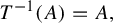$T^{-1}(A)=A,$ where A is a measurable subset of X, then either $\mu (A)=0$ or $\mu (X\setminus A)=0$ .

Given two measures $\mu $ and $\nu $ on the same space, we say $\nu $ is absolutely continuous with respect to $\mu $ if $\mu (A)=0 \implies \nu (A)=0$ , where $A \subseteq X$ . We denote this by $\nu \le \le \mu $ . If $\nu \le \le \mu $ and $\mu \le \le \nu $ , then we say the two measures are equivalent and write $\mu \sim \nu $ . We say equivalent measures are part of the same measure class [Reference Kesseböhmer, Munday and Stratmann21].

If two sets X and Y are equal up to a set of measure 0 using a given measure $\mu $ , that is, if $\mu (X \setminus Y)=0$ and $\mu (Y \setminus X)=0$ , then we write $X = Y \pmod \mu $ .

It is classical that the Gauss map on the unit interval is ergodic. In addition to the above reference, see Hensley [Reference Hensley15], and Rockett and Szüsz [Reference Rockett and Szusz23]

6.2 The jump transformation g

For the rest of this section, all the maps and domains will be in the sliced version. Thus, when we write T and $\triangle $ , we mean $T^S$ and $\triangle ^S$ , respectively.

This subsection is a straightforward generalization of the first three paragraphs of [Reference Messaoudi, Nogueira and Schweiger22, §4.1].

In keeping with [Reference Messaoudi, Nogueira and Schweiger22], we introduce the jump transformation g. This will be useful because it allows us to jump to the points in the triangle sequence where our guaranteed cell shrinkage (that is, our strings of zeros) occurs. Additionally, as a reminder, the original triangle map T is ergodic if and only if the sliced triangle map $T^S$ is ergodic.

First, define

$$ \begin{align*} \begin{aligned} \mathcal B_m &= \{\triangle(b_1, \ldots, b_m): \text{ the first appearance of a string of }n-1 \\&\qquad \text{zeros in the sequence of }b_j\text{ terms ends at }b_m;\ i=1,2,\ldots, n\} \end{aligned} \end{align*} $$

and

$$ \begin{align*}B_m = \bigcup_{E \in \mathcal B_m} E.\end{align*} $$

Thus, $\mathcal B_m$ is the set of all subcells of $\triangle $ consisting of points whose triangle sequences have the first string of $n-2$ consecutive zeros being $b_{m-(n-2)}=0$ , $b_{m-(n-3)}=0, \ldots , b_m=0$ , and $B_m$ is the cell consisting of their union. For these definitions to make sense, we need $m \ge n-2$ . By Corollary 4.2, we have that

$$ \begin{align*}\bigcup_m B_m=\triangle \pmod {\unicode{x3bb}}.\end{align*} $$

Note that mod $\unicode{x3bb} $ , the sets E such that 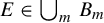$E \in \bigcup _m B_m$ form a partition $\mathcal {P}^{(1)}$ of $\triangle $ . We now define

$$ \begin{align*} g: \triangle \rightarrow \triangle, \quad g(u)=f^k(u)\ \ \text{ if } u \in B_k. \end{align*} $$

We now look at increasingly finer partitions of $\triangle ,$ defined inductively as follows. Once we have a partition $\mathcal {P}^{(k)}$ defined, we define $\mathcal {P}^{(k+1)}$ as the partition consisting of all intersections of sets $H \in \mathcal {P}^{(k)}$ and sets $g^{-1}(G)=\bigcup _m(f^{-m}(G) \cap B_m), G \in \mathcal {P}^{(k)}.$

In more plain language, $\mathcal {P}^{(1)}$ is the set of all

$$ \begin{align*}\triangle(b_0, \ldots, b_{m-n},b_{m-(n-1)},\underbrace{0,0,\ldots, 0}_{n-1 \text{ zeroes}}),\end{align*} $$

where all of the $b_i$ are positive, $\mathcal {P}^{(2)}$ is the set of all

$$ \begin{align*}\triangle(b_0, \ldots, b_{m},\underbrace{0,0,\ldots, 0}_{n-1 \text{ zeroes}}),c_0, \ldots, c_{0}, \ldots, c_{k},\underbrace{0,0,\ldots, 0}_{n-1 \text{ zeroes}})),\end{align*} $$

where all of the $b_i$ and $c_j$ are positive, $\mathcal {P}^{(2)}$ is the set of all corresponding cones with three ‘patches’ of $n-2$ zeros in a row, etc.

The key for us is that for all $\triangle (b_1, \ldots , b_m)\in \mathcal B_m, $ we have that not only is

$$ \begin{align*}g(\triangle(b_1, \ldots, b_m)) = \triangle,\end{align*} $$

but that the map g is one-to-one and onto. This will mean that for any cone $C\in \mathcal {P}^{(k)}$ ,

$$ \begin{align*}g(C)= \mathcal{P}^{(k-1)}, g^{(2)}(C)= \mathcal{P}^{(k-2)}, \ldots, g^{(k-1)}(C)= \mathcal{P}^{(1)}, g^{(k)}(C)= \triangle.\end{align*} $$

We have that

$$ \begin{align*}\bigcup_{C\in \mathcal{P}^k} C=\triangle \pmod {\unicode{x3bb}}.\end{align*} $$

As k increases, we have by Theorem 3.2 that the diameter of all the relevant cells tends to 0. Thus, $\mathcal C^{(k)} \uparrow \mathcal B$ , where $\mathcal B$ is the Borel algebra and the up arrow means $\mathcal C^{(k)}$ is an increasing sequence of sets whose limit as $k\rightarrow \infty $ is $\mathcal B$ .

We will be needing the following critical fact. If A is a subset with positive Lebesgue measure in $\triangle ,$ then there is k and a cone $C\in \mathcal {P}^k$ so that

$$ \begin{align*}\unicode{x3bb} (C\cap A) = \unicode{x3bb}(C),\end{align*} $$

meaning that C is contained in A almost everywhere.

To show ergodicity of T, all we need do is to show that the jump transformation g is ergodic, by the following lemma.

6.3 The jump transformation is ergodic

This is a straightforward generalization of [Reference Messaoudi, Nogueira and Schweiger22, Lemma 4.1].

We want to show that $g:\triangle \rightarrow \triangle $ is ergodic with respect to Lebesgue measure $\unicode{x3bb} .$

Start with a measurable set $\Omega $ of $\triangle $ with

$$ \begin{align*}g^{-1}(\Omega) = \Omega \quad\text{almost everywhere (a.e.).}\end{align*} $$

We want to show that

$$ \begin{align*}\unicode{x3bb}(\Omega) =0 \quad \mbox{or} \quad \Omega= \triangle\quad \mathrm{a.e.} \end{align*} $$

We will assume that $\unicode{x3bb} (\Omega ) \neq 0,$ as otherwise, we would be done. Suppose $ \Omega \neq \triangle , \mathrm {a.e.}$ Then, we must have that the complement has positive measure:

$$ \begin{align*}\unicode{x3bb}(\triangle -\Omega)>0.\end{align*} $$

All of our previous work in showing that the elements of the partitions $\mathcal {P}^{(k)}$ approach single points as $k\rightarrow \infty $ will mean that there must be a k and an element of $C\in \mathcal {P}^{(k)}$ so that C is contained in $\triangle -\Omega , \mathrm {a.e.}$ Thus, we must have that there is a $C\in \mathcal {P}^{(k)}$ for some k with

$$ \begin{align*}\unicode{x3bb}(\Omega \cap C) =0.\end{align*} $$

The next step is to show that for every $C\in \mathcal {P}^{(k)}$ for any k, we must have

$$ \begin{align*}\unicode{x3bb}(\Omega \cap C)>0,\end{align*} $$

giving us our needed contradiction.

Start with some $C\in \mathcal {P}^{(k)}$ . As $\Omega $ is an invariant set, we have

$$ \begin{align*}\Omega \cap C= g^{(-1)}\Omega \cap C = \cdots =g^{(-k)}\Omega \cap C. \end{align*} $$

We know then that

$$ \begin{align*}g^{(k)}(\Omega \cap C) = g^{(k)}( g^{(-k)}\Omega)\cap g^{(k)}(C) = \Omega. \end{align*} $$

Thus,

$$ \begin{align*}\unicode{x3bb}(\Omega \cap C) = \int_{\Omega} \mbox{Jac}(g^{(k)}) {d} \unicode{x3bb}.\end{align*} $$

Luckily, the Jacobian $\mbox {Jac}(g^{(k)})$ is not hard to calculate, as is discussed, again, in [Reference Messaoudi, Nogueira and Schweiger22]. Let $A=(A_0, \ldots , A_n) $ be the matrix describing the cone C. Then,

$$ \begin{align*} \unicode{x3bb}(\Omega \cap C) &= \int_{\Omega} \mbox{Jac}(g^{(k)}) {d} \unicode{x3bb}\\ &= \underset{\Omega }{\int} \frac{d\unicode{x3bb}}{(\|A_0\|x_0+\|A_1\|x_1+\cdots + \|A_n\|x_n)^{n+1}} \\ &\geq \frac{\unicode{x3bb}(\Omega)}{\|A_{\max}\|^{n+1}}\\ &>0, \end{align*} $$

where $\|A_{\max }\|:=\max _{1 \le i \le n} \|A_i\|$ .

We have our contradiction, meaning that the map g is indeed ergodic.

7.1 Invariant measures

We now know that the triangle map $T:\triangle \rightarrow \triangle $ , given by

$$ \begin{align*}T(x_1, \ldots, x_n) = \bigg(\frac{x_2}{x_1}, \ldots , \frac{x_n}{x_1}, \frac{1-x_1-b x_n}{x_1}\bigg)\end{align*} $$

for any $(x_1, \ldots , x_n) \in \triangle _b$ is ergodic with respect to Lebesgue measure. However, this is not an invariant measure, as for almost any set A of $\triangle $ , we have that

$$ \begin{align*}\unicode{x3bb}(A) \neq \unicode{x3bb}(T^{-1}(A)).\end{align*} $$

The natural question is to find an invariant measure that is absolutely continuous with respect to Lebesgue measure, a question both asked and answered by Gauss in the $n=1$ case, and known for $n=3$ [Reference Garrity14]. Our goal for this section is the following theorem.

Theorem 7.1. The invariant measure for the triangle map T in dimension n is

$$ \begin{align*}\frac{{d} \unicode{x3bb}}{x_1x_2\cdots x_{n-1}(1+x_n)}.\end{align*} $$

We will prove this using the rhetoric of the transfer operator. Recall that for a dynamical system with the map $T: X \rightarrow X$ , the transfer operator, denoted $\mathcal L$ or $\mathcal L_T$ , sends measurable functions on X to measurable functions on X such that for all measurable subsets A of X, we have

$$ \begin{align*}\int_{T^{-1}(A)}f(x)\mathop{dx}=\int_A\mathcal L_Tf(x)\, dx.\end{align*} $$

The transfer operator is a common tool for verifying candidate invariant measures, because an invariant measure must be an eigenfunction with largest eigenvalue 1 for the transfer operator corresponding to a given map. (For more on the background of transfer operators, see Hensley [Reference Hensley15], Iosifescu and Kraaikamp [Reference Iosifescu and Kraaikamp16], Kesseböhmer, Munday, and Stratmann [Reference Kesseböhmer, Munday and Stratmann21], and Schweiger [Reference Schweiger24], and for more general background, see Baladi [Reference Baladi5].)

Definition 7.2. The transfer operator $\mathcal L$ for any differentiable map T acting on a measurable real-valued function f is

$$ \begin{align*}\mathcal L (f)(p) = \sum_{q:T(q)=p} \frac{1}{|\text{Jac}(T(q))|}f(q) [14].\end{align*} $$

This section is a straightforward generalization of the $n=2$ case given in [Reference Garrity14]. Hence, we simply must calculate the transfer operator for the n-dimensional triangle map and then verify that our candidate function is an invariant measure. Since it does not require creative new ideas, we omit some of the background from dynamical systems.

We can directly calculate that

$$ \begin{align*}T^{-1}(x_1, \ldots, x_n)=\bigg( \frac{1}{1+kx_{n-1}+x_n},\frac{x_1}{1+kx_{n-1}+x_n},\ldots, \frac{x_{n-1}}{1+kx_{n-1}+x_n}\bigg). \end{align*} $$

(The method is to look at the homogeneous version of the triangle map, giving us that $T^H$ can be described as an $(n+1) \times (n+1)$ matrix. Then, the inverse of $T^H$ is simply the inverse of this matrix. To get $T^{-1}$ , we simply then ‘dehomogenize’, which in this case means divide by the first coordinate, giving us the above $T^{-1}.$ )

Then, we get that

$$ \begin{align*} &\mathcal Lf(x_1, \ldots, x_n) \\ & \quad = \sum_{k=0}^\infty \frac{1}{(1+kx_{n-1}+x_n)^{n+1}}f\bigg(\frac{1}{1+kx_{n-1}+x_n}, \frac{x_1}{1+kx_{n-1}+x_n}, \ldots \frac{x_{n-1}}{1+kx_{n-1}+x_n}\bigg). \end{align*} $$

(Again, while the calculations are straightforward, though a bit messy, they are completely analogous to the $n=2$ case that is worked out in [Reference Garrity14].) As for the proof of Theorem 7.1, we must show that

$$ \begin{align*}\mathcal L \bigg( \frac{1}{x_1x_2\cdots x_{n-1}(1+x_n)} \bigg) = \frac{1}{x_1x_2\cdots x_{n-1}(1+x_n)}.\end{align*} $$

This is a straightforward calculation, though a bit messy. It will come down to a telescoping series.

Of course, this begs the question of how we found the invariant measures. We simply guessed. There are two other non-guess approaches. One could use the natural extensions of the triangle map, which has implications for the link with integer partitions. This is currently being developed in [Reference Fox and Garrity12]. The second approach is to use the dual algorithm. This was the approach suggested by the referee. For background on the dual algorithm, see [Reference Schweiger24, Definition 27].

7.2 Normalizing constant

For the simplex $\triangle $ in ${\mathbb R}^n$ , we have that

$$ \begin{align*}\int_{\triangle} \frac{{d} \unicode{x3bb}}{x_1x_2\cdots x_{n-1}(1+x_n)}\neq 1.\end{align*} $$

This subsection finds for each n,

$$ \begin{align*}C_n = \int_{\triangle} \frac{{d} \unicode{x3bb}}{x_1x_2\cdots x_{n-1}(1+x_n)}.\end{align*} $$

In the $n=1$ case (the Gauss map), we have the classical

$$ \begin{align*}C_1=\int_0^1 \frac{1}{1+x}\,dx =\log(2).\end{align*} $$

Theorem 7.3. For $n\ge 2$ , the normalizing constant for the invariant measure of the triangle map in ${\mathbb R}^{n+1}$ is

$$ \begin{align*}C_n=\frac{2^{n-1}-1}{2^{n-1}}\zeta(n),\end{align*} $$

where $\zeta (n)$ is the Riemann zeta function.

The proof is a calculation, using at the end that

$$ \begin{align*}\sum_{k=1}^\infty \frac{1}{(2k)^n} = \frac{1}{2^n}\zeta(n).\end{align*} $$

8.1 Definition of the slow triangle map

We again start with

$$ \begin{align*}\triangle = \{ (x_1, \ldots, x_n) \in {\mathbb R}^n:1\geq x_1 \cdots \geq x_n\geq 0\}.\end{align*} $$

We now partition this simplex into two sub-simplices:

$$ \begin{align*}\triangle_0 &= \{ \mathbf{x}\in \triangle: 1<x_1 + x_n \}, \\ \triangle_1&= \{ \mathbf{x}\in \triangle: x_1+x_n<1 \}. \end{align*} $$

Definition 8.1. The slow triangle map

$$ \begin{align*}t:\triangle \rightarrow \triangle\end{align*} $$

is defined as

$$ \begin{align*} t(\mathbf{x}) &= \begin{cases} t_0(\mathbf{x}) & \mbox{if } \mathbf{x} \in \triangle_0, \\ t_1(\mathbf{x}) & \mbox{if } \mathbf{x} \in \triangle_1,\end{cases}\\[4pt] &= \begin{cases} \bigg( \dfrac{x_2}{x_1}, \ldots, \dfrac{x_n}{x_1}, \dfrac{1-x_1}{x_1} \bigg) & \mbox{if } \mathbf{x} \in \triangle_0, \\ \bigg( \dfrac{x_1}{1-x_n}, \ldots, \dfrac{x_n}{1-x_n} \bigg) & \mbox{if } \mathbf{x} \in \triangle_1.\end{cases}\ \end{align*} $$

When $n=1$ , this is the classical Farey map.

Definition 8.2. The slow triangle sequence for any $\mathbf {x}\in \triangle $ is a sequence

$$ \begin{align*}(i_0,i_1, \ldots)\end{align*} $$

of integers $i_k$ , each of which is zero or one, such that

$$ \begin{align*}\mathbf{x }\in \triangle_{i_0}, t(\mathbf{x}) \in \triangle_{i_1}, t^{(2)}(\mathbf{x}) \in \triangle_{i_2}, \ldots .\end{align*} $$

There is an easy way to pass from the slow triangle sequence for any $\mathbf {x}\in \triangle $ to the (fast) triangle sequence given in Definition 2.8. For any $\mathbf {x}\in \triangle _b$ , we have

$$ \begin{align*}T(\mathbf{x }) = t_0\circ t_1^{(b)} (\mathbf{x}).\end{align*} $$

Thus, to go from a slow triangle sequence $(i_0,i_1, \ldots )$ to the (fast) triangle sequence, we simply need to concatenate the $1$ terms and add one to the number of $1$ terms. Thus, a slow triangle sequence

$$ \begin{align*}(1,1,0,1,1,1,0,0,0,1,1,0, \ldots )\end{align*} $$

is the same as the fast triangle sequence

$$ \begin{align*}(3, 4, 1,1,3,\ldots).\end{align*} $$

8.2 The invariant measure for the slow case

As in §7, there is an invariant for the map t. As the arguments are similar to that earlier section, we will only sketch the results.

Proposition 8.3. The measure

$$ \begin{align*}{d} \nu = \frac{1}{x_1x_2\cdots x_n}\,{d} \unicode{x3bb}\end{align*} $$

is an invariant measure for the slow triangle map t. Hence, for all measurable sets A in $\triangle $ , we have

$$ \begin{align*}\nu(A) = \int_A {d} \nu = \int_{t^{(-1)} A}\,{d} \nu = \nu(t^{(-1)} (A)).\end{align*} $$

We need to show that the function $1/(x_1\cdots x_n)$ is an eigenfunction with eigenvalue one of the transfer operator

$$ \begin{align*}\mathcal L f(x_1, \ldots, x_n) = \lvert\det J_0\rvert f(T_0^{-1}(x_1,\ldots, x_n))+\lvert\det J_1\rvert f(T_1^{-1}(x_1,\ldots, x_n)).\end{align*} $$

By direct calculation, we have

$$ \begin{align*} \mathcal L f(\mathbf{x}) &= \frac{1}{(1+x_n)^{n+1}}f(T_0^{-1}(\mathbf{x}))+\frac{1}{(1+x_n)^{n+1}}f(T_1^{-1}(\mathbf{x}))\\&= \frac{1}{(1+x_n)^{n+1}} f\bigg( \frac{1}{1+x_n}, \frac{x_1}{1+x_n}, \ldots , \frac{x_{n-1}}{1+x_n}\bigg) \\& \quad + \frac{1}{(1+x_n)^{n+1}} f\bigg( \frac{x_1}{1+x_n}, \frac{x_2}{1+x_n}, \ldots , \frac{x_{n}}{1+x_n}\bigg). \end{align*} $$

Showing that

$$ \begin{align*} \mathcal L \bigg( \frac{1}{x_1x_2\cdots x_n} \bigg)= \frac{1}{x_1x_2\cdots x_n}\end{align*} $$

is a calculation.

As with the fast version, we simply guessed the invariant measures. Additionally, as with the fast version, we could also have used the natural extensions of the slow triangle map [Reference Fox and Garrity12] or the dual algorithm of the slow map (which was suggested by the referee).

We cannot find the normalizing constant for this measure, as it is infinite on $\triangle _1$ . This is reflected, for example, in the $n=1$ case (the Farey map), which has an indifferent fixed point at the origin. Similarly, the origin is an indifferent fixed point for the slow triangle map in any dimension and that the invariant measure is infinite on all of the $\triangle _1$ . This should lead to many interesting technical problems and issues.

8.3 The induced system

Our goal is to show that the slow triangle map $t:\triangle \rightarrow \triangle $ is ergodic for any dimension. No doubt we could prove this directly, mimicking all the work that we did earlier. However, instead, we will show how the ergodicity of the triangle map T will imply the ergodicity of the map t. We will overwhelmingly be following the argument given by Kessebömer, Munday, and Stratmann [Reference Kesseböhmer, Munday and Stratmann21, Ch. 2], where they show that the ergodicity of the Gauss map (the $n=1$ triangle map) implies the ergodicity of the Farey map (the $n=1$ slow triangle map).

By [Reference Kesseböhmer, Munday and Stratmann21, Definition 2.2.12], the set $\triangle _0 = \{ \mathbf {x}\in \triangle : 1<x_1 + x_n \}$ will be a sweep-out set if $\nu (\triangle _0)<\infty $ and

$$ \begin{align*}\nu\bigg(\triangle - \bigcup_{k=0}^{\infty} T^{(-k)} (\triangle_0)\bigg) =0.\end{align*} $$

Proof. It is a calculation that

$$ \begin{align*}\nu(\triangle_0) = \int_{\triangle_0} \frac{1}{x_1x_2\cdots x_n}\,{d}x_1 \cdots \,{d}x_n\end{align*} $$

is finite.

Now, it is straightforward to show that both $t_0:\triangle \rightarrow \triangle $ and $t_1:\triangle \rightarrow \triangle $ are onto maps. By direct calculation, we have that

$$ \begin{align*}t_1^{(-1)} (x_1, \ldots, x_n ) = \bigg( \frac{x_1}{1+x_n}, \ldots, \frac{x_n}{1+x_n} \bigg).\end{align*} $$

We know that the vertices of $\triangle _0$ are

$$ \begin{align*} v_1&= (1, 0, \ldots, 0), \\ v_2 &= (1, 1, 0, \ldots, 0), \\ &\ \ \vdots \\ v_{n-1} &= (1, 1, \ldots, 1, 0), \end{align*} $$

and

$$ \begin{align*} w_1&= (1/2, 1/2, \ldots, 1/2), \\ w_2 &= (1, 1, \ldots, 1). \end{align*} $$

We have that $t_1^{(-1)}$ acting on any of the vertices $v_i$ leaves $v_i$ alone. However,

$$ \begin{align*} t_1^{(-1)}(w_1)&= (1/3, 1/3, \ldots, 1/3) ,\\ t_1^{(-1)}(w_2) &= (1/2, 1/2, \ldots, 1/2). \end{align*} $$

In general, 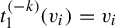$t_1^{(-k)}(v_i) = v_i$ and

$$ \begin{align*} t_1^{(-k)}(w_1)&= (1/(k+2), 1/(k+2), \ldots, 1/(k+2), \\ t_1^{(-k)}(w_2) &= (1/(k+1), 1/(k+1), \ldots, 1/(k+1)). \end{align*} $$

This shows that $\triangle _0$ is a sweep-out set.

In the context of the slow triangle map, [Reference Kesseböhmer, Munday and Stratmann21, Definition 2.4.25] leads to the following definition.

Definition 8.5. The induced map of the slow triangle map t on $\triangle _0$

$$ \begin{align*}t_{\triangle_0}: \triangle_0 \rightarrow \triangle_0 \end{align*} $$

is

$$ \begin{align*}t_{\triangle_0}(x):=t^{\varphi(x)}(x),\end{align*} $$

where, in turn,

$$ \begin{align*}\varphi(x)=\inf\{k\ge 1: n^k(x) \in \triangle_0\}.\end{align*} $$

With the eventual goal of ergodicity for t, we have the following proposition.

This is simply [Reference Kesseböhmer, Munday and Stratmann21, Proposition 2.4.28].

Now, the triangle map t is non-singular ([Reference Kesseböhmer, Munday and Stratmann21, Definition 2.2.4]) if for all measurable sets A with measure zero, we have that the measure of $t^{(-1)}(A)$ also has measure zero. However, this follows from the existence of the invariant measure $\nu $ .

The map t is conservative follows from $t_{\triangle _0}$ being conservative, which follows immediately from [Reference Kesseböhmer, Munday and Stratmann21, Proposition 2.2.23], and from [Reference Kesseböhmer, Munday and Stratmann21, Proposition 2.4.27].

8.4 Ergodicity of induced map

Thus, we have to show that $t_{\triangle _0}:\triangle _0 \rightarrow \triangle _0$ is ergodic.

We need to link the induced system to the original triangle map T, which we know to be ergodic.

Proposition 8.7. The dynamical system

$$ \begin{align*}t_{\triangle_0}:\triangle_0 \rightarrow \triangle_0\end{align*} $$

with invariant measure $\nu |_{\triangle _0}$ is measure-theoretically isomorphic to the dynamical system

$$ \begin{align*}T:\triangle \rightarrow \triangle\end{align*} $$

with invariant measure $\mu .$

This will immediately give us that the slow triangle map is ergodic.

As for measure-theoretically isomophic, this means the following. We have to construct a map

$$ \begin{align*}\psi:\triangle_0 \rightarrow \triangle\end{align*} $$

so that the diagram

$$ \begin{align*}\begin{array}{ccc} \triangle_0 & \xrightarrow{t_{\triangle_0}} & \triangle_0 \\ \psi \downarrow & & \downarrow \psi \\ \triangle & \xrightarrow{T} & \triangle \end{array}\end{align*} $$

is commutative and so that, for all measurable sets B in $\triangle ,$ we have

$$ \begin{align*}\nu|_{\triangle_0}\circ \psi^{-1}(B) = \mu(B).\end{align*} $$

Proof. Simply define

$$ \begin{align*}\psi = t_0.\end{align*} $$

Then, the argument is the same as that given in [Reference Kesseböhmer, Munday and Stratmann21, proof of Proposition 2.4.31], which is for the $n=1$ case.