1 Introduction
When the interface between a conducting liquid and an insulating fluid is charged at a voltage
 $V$
relative to neighbouring electrodes, the resulting electrostatic stresses deform the surface. Past a geometry-dependent critical voltage
 $V^{\ast }$
, where electrostatic stresses overcome capillary stresses, the initially static and convex interface becomes unstable and develops a conical tip, or Taylor cone (Taylor Reference Taylor1964), from which charged liquid is ejected. In the best-studied mode of emission, the cone-jet regime (Cloupeau & Prunet-Foch Reference Cloupeau and Prunet-Foch1989), a steady jet issues from the apex of the cone, subsequently breaking into an electrospray of drops with relatively uniform diameter
 $d_{p}$
. Most singular is the fact that, in liquids of high electrical conductivity
 $K$
(
 ${\sim}1~\text{S}~\text{m}^{-1}$
), this diameter may be 10 nm or less. The main variables controlling
 $d_{p}$
and the emitted electrical current
 $I$
are
 $K$
, the flow rate
 $Q$
of liquid pushed through the jet and the surface tension
 $\unicode[STIX]{x1D6FE}$
, with the following approximate scaling laws having been proposed (Fernandez de la Mora & Loscertales Reference Fernandez de la Mora and Loscertales1994):
 $$\begin{eqnarray}\displaystyle & I=f(\unicode[STIX]{x1D700})(\unicode[STIX]{x1D6FE}KQ)^{1/2} & \displaystyle\end{eqnarray}$$
 $$\begin{eqnarray}\displaystyle & d_{p}=g(\unicode[STIX]{x1D700})(Q\unicode[STIX]{x1D700}_{o}/K)^{1/3}. & \displaystyle\end{eqnarray}$$
Although the applied voltage has a minor effect on both
 $I$
and
 $d_{p}$
, it still plays a crucial role because a steady cone-jet can be formed only within a certain
 $K$
-dependent stability island in (
 $Q,V$
) space. The smallest drop diameter attainable is of considerable practical importance, and is accordingly determined by the smallest possible flow rate
 $Q_{min}$
, in turn fixed by the form of the stability island (Cloupeau & Prunet-Foch Reference Cloupeau and Prunet-Foch1989). How to widen this island towards smaller
 $Q$
values is therefore most relevant and will be pursued here by the application of magnetic fields.
The approach was inspired by a series of recent studies on simultaneously magnetized and electrified liquid interfaces (magnetoelectrosprays) aimed at overcoming a major limitation of electrosprays for most applications other than mass spectrometry: the rather small throughput of drops that may be produced, especially at small drop sizes. Instead of the microfabrication techniques previously pursued to produce dense arrays with thousands of individual emitters (Courtney, Li & Lozano Reference Courtney, Li and Lozano2012), King et al. (Reference King, Meyer, Hopkins, Hawkett and Jain2014) have proposed to exploit the natural tendency of ferrofluids subject to magnetic fields to develop numerous pointed tips (Gollwitzer et al.
Reference Gollwitzer, Matthies, Richter, Rehberg and Tobiska2007). Magnetic tips differ in two respects from Taylor cones arising in conducting liquids. First, they tend to be static, not emitting liquid, and second their tip structure does not appear to the naked eye to be conical. The electric/magnetic analogy is more appropriate in the case of dielectric liquids, also static, where a transition between rounded and conical tips theoretically takes place at sufficiently strong fields, provided the dielectric constant
 $\unicode[STIX]{x1D700}$
exceeds a critical value
 $\unicode[STIX]{x1D700}^{\ast }=17.59864$
(Brancher & Zouaoui Reference Brancher and Zouaoui1987; Ramos & Castellanos Reference Ramos and Castellanos1994). A most interesting literature exists for both ferrofluids (Bacri & Salin Reference Bacri and Salin1982; Sero-Guillaume et al.
Reference Sero-Guillaume, Zouaoui, Bernardin and Brancher1992) and dielectrics (Wohlhuter & Basaran Reference Wohlhuter and Basaran1992) describing critical shape transitions from compact to elongated forms, sometimes with the formation of conical tips (Stone, Lister & Brenner Reference Stone, Lister and Brenner1999; Lavrova et al.
Reference Lavrova, Matthies, Mitkova, Polevikov and Tobiska2006).
King’s (Reference King2014) original proposal involves first forming magnetically a static set of suitably arranged tips in an electrically conducting ferrofluid, followed by the application of an electric field to turn each of the pre-existing static points into dynamic cone-jets. This magnetoelectrospraying approach opens up a new and considerably richer range of possibilities to control not just the number and density of emitters, but perhaps also the characteristics of the emission region. Our initial motivation for the present study was the hope that magnetic fields would widen the range of stability of electrified liquids, limited in part by loss of electrostatic equilibrium of surface charges caused by fluid motion towards the jet. If the capillary pressure were compensated by magnetic in addition to electric stresses, a much smaller surface charge would be required to form a conical tip, perhaps increasing jet stability. Also, given a relatively sharp non-emitting magnetic tip, one could alternate the electrical polarity without resulting in collapse of the tip, except in a very small volume at its apex. Since the time required to reinstate the electrical emission is proportional to the square root of the oscillating tip volume, the polarity could be changed at high frequency.
These hypothetical advantages of electrified/magnetized liquid points, however, demand that the magnetically stabilized tip be very sharp, so a first question to be tackled is how sharp these magnetized tips may be made in practice. A finite curvature limit exists in the case of real Taylor cones, set by the finite values of
 $K$
and
 $Q$
. This limitation follows from the fact that the problem is dynamic. But no comparable restriction exists for magnetic tips, which are static. Several previous theoretical studies have in fact predicted infinitely sharp magnetized tips (Brancher & Zouaoui Reference Brancher and Zouaoui1987; Ramos & Castellanos Reference Ramos and Castellanos1994; Stone et al.
Reference Stone, Lister and Brenner1999), even though in practice one always sees finite curvatures. We have not found in the literature a clear explanation for this discrepancy, but one has been recently provided privately by Professor Higuera (Polytechnical University, Madrid). Because the linear magnetic response model used in these three theoretical studies (Brancher & Zouaoui Reference Brancher and Zouaoui1987; Ramos & Castellanos Reference Ramos and Castellanos1994; Stone et al.
Reference Stone, Lister and Brenner1999) is valid only at magnetizations well below saturation, the maximal tip curvature may be at most that balancing the magnetic stress under saturation conditions. A rough estimate for the tip radius would then be
 $R\sim 4\unicode[STIX]{x1D6FE}/(\unicode[STIX]{x1D707}_{o}M_{sat}^{2})$
, where
 $M_{sat}$
is the saturation magnetization of the ferrofluid. Using as a reference Ferrotec’s EMG 9900 ferrofluid (
 $M_{sat}=7.8\times 10^{4}~\text{A}~\text{m}^{-1}$
) and a typical value
 $\unicode[STIX]{x1D6FE}=0.03~\text{N}~\text{m}^{-1}$
, we find
 $R\sim 15~\unicode[STIX]{x03BC}\text{m}$
. In contrast, electrified tip radii for highly conducting liquids (
 $K\sim 1~\text{S}~\text{m}^{-1}$
) may be as small as 10 nm. Higuera’s hypothesis is confirmed by a recent study appeared after submission of our own, where magnetized drop shapes are computed for a magnetic fluid model including saturation effects, resulting always in finite curvatures (Rowghanian, Meinhart & Campàs Reference Rowghanian, Meinhart and Campàs2016). These considerations would have lead us to abandon all hope of discovering relevant magnetic effects on the stability range of conventional electrified liquid cones. Fortunately, when we became aware of this limitation, our experimental study had already shown that such effects are substantial.
2 Materials and methods
2.1 Materials
2.1.1 Sulfolane ferrofluid
The required electrosprayable ferrofluid needs to have a finite conductivity, for which aqueous ferrofluids seemed at first sight suitable. However, commercial aqueous ferrofluids stabilize the magnetite suspension with high concentrations of ionic surfactants, and therefore have high electrical conductivities
 $K$
. But stable electrosprays of high
 $K$
liquids require very small liquid flow rates, with large residence times of the liquid in the meniscus, which for volatile liquids like water lead to particle destabilization and precipitation. Commercial oil-based ferrofluids have also been electrosprayed (Uehara, Itoga & Nishiyama Reference Uehara, Itoga and Nishiyama2015), but their rather low conductivities result in jets tens of microns wide. Such jets may be generated by simpler means, and also require an inconveniently large consumption of ferrofluid. In addition, our main application is to electrical propulsion in vacuum, for which a low volatility solvent is essential. In a separate article we will describe low volatility glycerol-based ferrofluids. Here we study less viscous ferrofluids of low volatility formed by mixing sulfolane with the room temperature molten salt ethylammonium nitrate (SF/EAN) (Alonso-Matilla et al.
Reference Alonso-Matilla, Fernandez-Garcia, Congdon and Fernandez de la Mora2014). The new SF-based ferrofluids are vacuum compatible and freely miscible with EAN, remaining stable over an extremely wide range of electrical conductivities.
2.1.2 Synthesis
Dimethyl acrylamide (DMAm, Aldrich) was passed through an inhibitor removal column (Aluminium oxide, Aldrich). Acrylic acid (AA, Aldrich), 4,
 $4^{\prime }$
-azobis (4-cyanovaleric acid) (V-501, Wako), sulfolane (Ajax, 97 %), 1,4-dioxane (Merck, 99 %), sodium hydroxide (NaOH, Aldrich) and RAFT agent 2-
 $\{$
[(butylsulfanyl)carbonothioyl]sulfanyl
 $\}$
propanoic acid (BuPAT, DuluxGroup Australia) were used as received. The aqueous dispersion of iron oxide nanoparticles was obtained from Sirtex Medical Limited (Sirtex NPs). Deionized water was used in all experiments.
(
 $\text{RAFT}\text{-}\text{AA}_{10}\text{-}\text{b}\text{-}\text{DMAm}_{60}$
) was prepared as reported previously (Bryce et al.
Reference Bryce, Pham, Fong, Jain, Pan, Whan, Hambley and Hawkett2013). Monomers monoacryloxyethyl phosphate and acrylamide in the reported synthesis were replaced, on a mole-for-mole basis, with acrylic acid and N,N-dimethylacrylamide, respectively to prepare the stabilizer for the sulfolane-based ferrofluid. In a typical reaction, DMAm (6.46 g, 65.20 mmol), V-501 (0.03 g, 0.11 mmol), and BuPAT (0.26 g, 1.09 mmol) were added to a 100 ml round-bottomed flask containing a mixture of dioxane (10 g) and water (10 g). The mixture was held at
 $70\,^{\circ }\text{C}$
for 12 h under a nitrogen atmosphere and then cooled to room temperature. Acrylic acid (0.78 g, 10.9 mmol) and V-501 (0.03 g, 0.11 mmol) were added, and the reaction mixture was heated for another 4 h at
 $70\,^{\circ }\text{C}$
under nitrogen. At the end of this step, a block copolymer of nominal composition, poly(AA
 $_{10}$
-b-DMAm
 $_{60}$
), was obtained as a 31 % solids solution.
An aqueous dispersion of sterically stabilized Sirtex nanoparticles (NPs) was synthesized in water as reported previously (Jain et al.
Reference Jain, Wang, Jones, Hawkett and Warr2010) and the sulfolane ferrofluid was prepared in a similar manner to that used for preparation of an EAN-based ionic liquid ferrofluid (Jain et al.
Reference Jain, Wang, Hawkett and Warr2011). A dispersion of sterically stabilized Sirtex NPs in 50 : 50 (w/w) water:ethanol was mixed with sulfolane, followed by ultrasonication for 2 min. Water and ethanol were then removed by rotary evaporation. The final composition of the ferrofluid was determined by TGA (PerkinElmer Pyris 1) and found to be: iron oxide nanoparticles 20.5 %; polymeric stabilizer 3.5 %; water 12 % and sulfolane 64 % by weight. All the samples were heated to
 $105\,^{\circ }\text{C}$
and equilibrated at that temperature to remove residual solvent prior to analysis, then ramped up (
 $20\,^{\circ }\text{C}~\text{min}^{-1}$
) to
 $750\,^{\circ }\text{C}$
under a nitrogen atmosphere (
 $20~\text{ml}~\text{min}^{-1}$
). The Pyris Manager software was used to calculate the mass lost.
The mean diameter and polydispersity of the polymer-stabilized nanoparticles in aqueous dispersion was determined by dynamic light scattering (Malvern Instruments Zetasizer nano) to be 54.6 nm and 0.15 nm, respectively.
The magnetic properties of the sulfolane ferrofluid were measured in the liquid state at room temperature using a Quantum Design vibrating sample magnetometer (VSM) with a 9 T electromagnet. The magnetic moment was measured over a range of applied fields from
 $-10$
to
 $+10$
kOe (
 $\pm 800~\text{kA}~\text{m}^{-1}$
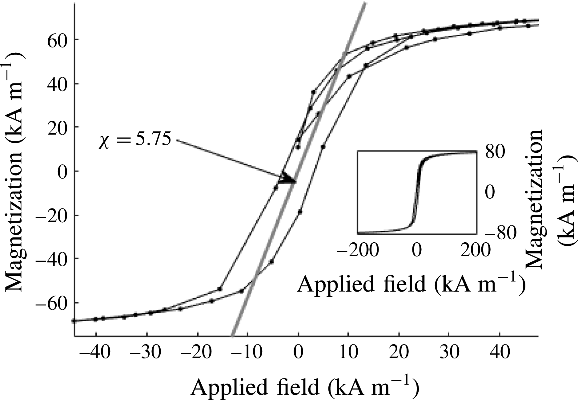
) with a sensitivity of 0.0002 emu. The magnetization curve of the sulfolane ferrofluid is shown in figure 1. The mass saturation magnetization of the sulfolane ferrofluid (
 $M_{sat}=58.5~\text{emu}~\text{g}^{-1}$
) was 18.3 % lower than that of pure maghemite Sirtex NPs (
 $M_{sat}=71.6~\text{emu}~\text{g}^{-1}$
) due to the reaction of the stabilizer anchor groups with the surface of the magnetic particles. The volumetric saturation magnetization field of the sulfolane ferrofluid is
 $73~\text{kA}~\text{m}^{-1}$
.
Magnetization curves of sulfolane ferrofluid at room temperature. Inset: broader view of ferrofluid magnetization presented to highlight large field magnetization saturation.

2.1.3 Sample composition and properties
This study focuses on two compositions of the sulfolane ferrofluid mixed with ethyl ammonium nitrate (EAN). Table 1 shows the two samples’ relevant properties and capillary geometries used. A larger diameter capillary is necessary for the lower conductivity liquid in order to accommodate the higher flow rates required to form a stable Taylor cone.
Ferrofluid properties.

Concentrations of EAN are chosen to cover a large range of electrical conductivities and liquid flow rates. The viscosity is measured with the time required to fill the capillary by integrating the Poiseuille pipe equation
 $$\begin{eqnarray}\unicode[STIX]{x1D707}=\frac{\unicode[STIX]{x0394}Pd_{cap}^{2}}{16L_{cap}^{2}}t,\end{eqnarray}$$
where
 $\unicode[STIX]{x1D707}$
is the dynamic viscosity,
 $t$
is the time required to fill the capillary,
 $d_{cap}$
is the diameter of the capillary,
 $L_{cap}$
is the length of the capillary and
 $\unicode[STIX]{x0394}P$
is the pressure above atmospheric applied to the vial acting as liquid reservoir. Equation (2.1) is the Washburn equation neglecting the capillary pressure jump (
 ${\sim}47~\text{mbar}$
), a point justified because
 $\unicode[STIX]{x0394}P$
was 1 bar.
The conductivity of the liquids is inferred from the ohmic resistance of a capillary (of known geometry) filled with ferrofluid. The resistances of the two capillaries used (when filled) are
 $1.3~\text{G}\unicode[STIX]{x03A9}$
and
 $20~\text{G}\unicode[STIX]{x03A9}$
for samples A and B respectively. The voltage drop
 $V_{drop}$
across the line during electrospray operation is determined by the measured current and bulk conductivity. The maximal voltage drops i.e. the voltage drop caused by the highest current across lines A and B are 247 volts and 1400 volts respectively. The reported tip voltage is the vial voltage minus
 $V_{drop}$
. Since the initial ferrous particle concentration is set in the base ferrofluid sample, susceptibility in sample A is presumed to be 85 % of that in sample B, or
 $3.43\times 10^{-3}~\text{m}^{3}~\text{kg}^{-1}$
.
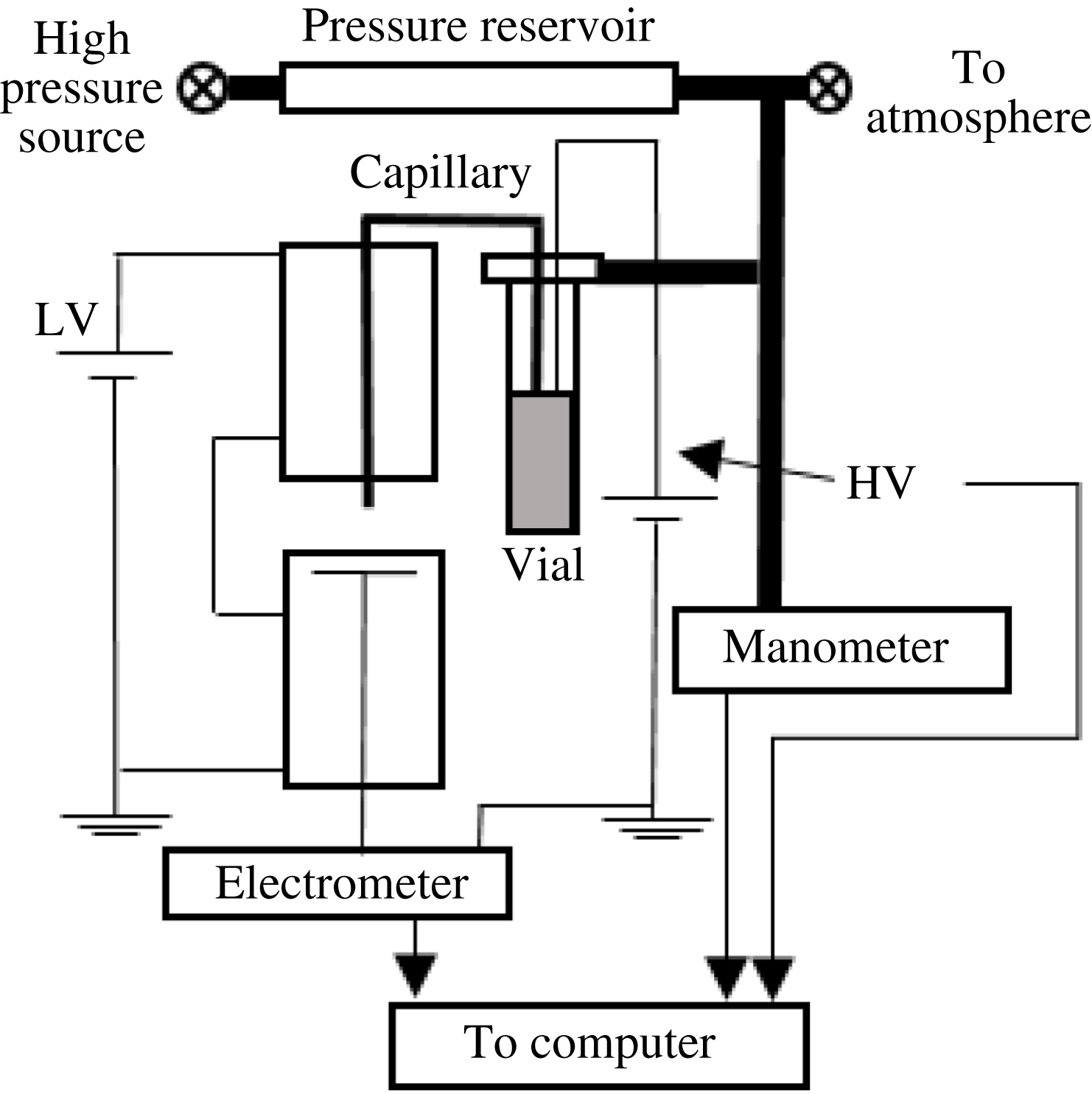
Schematic of experimental set-up. A gas tank connected to the ferrofluid reservoir is initially pressurized with air and slowly drained to scan over the liquid flow rate. High voltage is applied to the ferrofluid reservoir. A collector plate is virtually grounded through an electrometer. A voltage (300 V) is applied across two solenoids (with non-ferrous cores) connected in series to apply a homogeneous magnetic field to the space surrounding the capillary. The gas pressure, capillary voltage and spray current are automatically recorded.

2.2 Experiment
2.2.1 Electrospray parameter control
Figure 2 shows a schematic of the experimental set-up.
Ferrofluid is forced through a silica capillary into the magnetizable electrospray chamber by applying pressure above atmosphere to the vial from which it is supplied. The vial is kept at the same elevation as the electrospray chamber. Pressure above atmospheric is measured with a MPX5500 pressure transducer, read and stored via an Arduino Uno 10 bit DAQ. We calculate the volumetric flow rate from the Poiseuille pipe equation. For this relation to be valid, one needs to ensure the applied pressure greatly exceeds the electrostatic pulling pressure of the meniscus, of the order of the capillary pressure given by
 $$\begin{eqnarray}P_{cap}=\frac{4\unicode[STIX]{x1D6FE}}{d_{cap}}.\end{eqnarray}$$
The assumption is justified because the surface tension of the liquid
 $\unicode[STIX]{x1D6FE}$
takes at most the value for sulfolane, with
 $P_{cap}<47~\text{mbar}$
, while the lowest pressures used to force flow exceed 250 mbar.
High voltage is supplied to the vial reservoir so that charge reaches the capillary tip via conduction through the liquid. The fluid’s bulk conductivity is measured from the resistance of a clean capillary filled with the ferrofluid. The grounding plate consists of a brass tube topped by an aluminium mesh and filled with absorbent material to convect away emitted ferrofluid.
2.2.2 Magnetic field
This study utilized a solenoid to create a uniform magnetic field in the region surrounding the Taylor cone. This uniformity moderates the effects from the Kelvin body force
 $$\begin{eqnarray}F=\unicode[STIX]{x1D707}_{0}M\boldsymbol{\cdot }\unicode[STIX]{x1D735}H,\end{eqnarray}$$
which would be more prevalent if a permanent magnet were used. The applied field is calculated from the field generated by a solenoid
 $$\begin{eqnarray}H=nI,\end{eqnarray}$$
where
 $I$
, the current through the solenoids, is measured by a multimeter and
 $n$
is the number of turns per unit length. Here, two solenoids 4.47 cm in length with 10 000 turns of 35 gauge magnet wire each were placed in series with a small viewing gap between them (8 mm axial separation). These solenoids are kept in alignment by a brass tube (1.9 cm outer diameter) snugly fit concentrically. Because the core is open air outside the very narrow channel of magnetizable ferrofluid, the permeability of the core is taken as that of free space.
The external temperature and current of the solenoids during magnetized trials were
 $50\,^{\circ }\text{C}$
and 105 mA. This gives an applied field of
 $23\,490~\text{Am}^{-1}$
, which magnetizes the ferrofluid to 96.9 % of the saturation magnetization. To control for thermal effects introduced by solenoid power dissipation, an external fan array cools the coils and a sheath gas at low velocity is introduced around the Taylor cone. The gas temperature is controlled by power supplied to upstream thermal blankets to maintain a set temperature measured by a thermocouple near the capillary tip (located approximately 5 mm away). The internal sheath gas flow is held at
 $29\,^{\circ }\text{C}$
near the capillary tip for all trials, magnetized and non-magnetized.
2.3 Methods
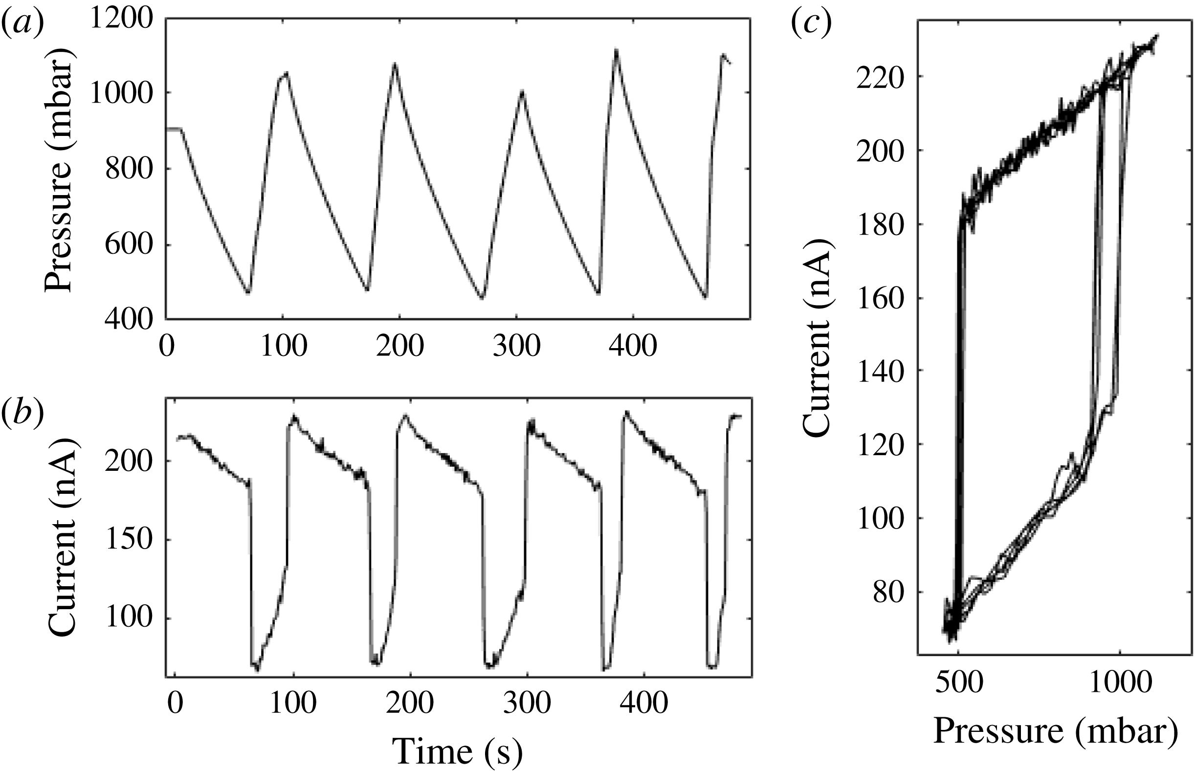
The emitted current is measured with a floating electrometer connected to the DAQ through a high voltage isolation amplifier and calibrated with a multimeter. To evaluate the boundary of the stability island for the cone-jet mode, a liquid flow rate considerably larger than the minimum at which the cone jet is stable is first established by applying a suitably high pressure to the vial. This flow rate is then reduced at approximately
 $1~\text{pl}~\text{s}^{-2}$
by lessening the pressure on the vial. The rate of pressure reduction is established by connecting the liquid reservoir to a pressurized gas tank with a controlled leak based on a partially open valve discharging into the atmosphere. The flow rate is thus slowly reduced until the cone destabilizes. Destabilization is quantified by a sharp drop in current and qualitatively confirmed by sight. After destabilization, pressure is quickly resupplied to the vial until the cone is re-established. This process is repeated fivefold to verify the reproducibility of the cycle at each voltage, magnetic field and liquid. This procedure effectively establishes the boundary of the stability island where the flow rate at a given voltage is minimized. Figure 3 shows a representative sample of the raw measured data, displaying the level of repeatability of the currents and the smallest flow rate at which the steady cone loses stability and the current collapses.
Raw data collected. (a) The pressure applied to the ferrofluid vial decays and is replenished; (b) the spray current tracks the applied pressure, and discontinuously drops when the cone destabilizes; (c) the current–flow rate relation drawn from their time relations shows the characteristic hysteresis of Taylor cones and the reproducibility of destabilization.

An alternative approach to determine the stability island was also used. At a flow rate reasonably far from the minimum for which the emission is stable over a wide range of applied voltages, we fix the reservoir pressure, and then decrease the voltage slowly until the cone destabilizes.
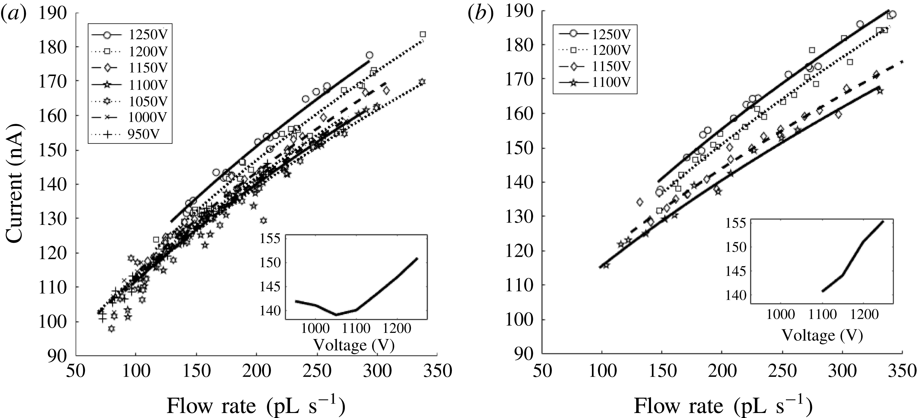
Aggregate Taylor cone current–flow rate relations for all voltages in sample A. Trend lines are linear regression curves (between
 $I^{2}$
and
 $Q$
) for many more data taken than the few representative data shown. (a) A 295 Gauss magnetic field applied coaxial with the capillary; (b) no magnetic field applied. Inset figures show current–voltage behaviour at
 $200~\text{pl}~\text{s}^{-1}$
(extracted from curve fit in main window). For increased clarity the figure shows only 5 % of the data.

3 Results
Figure 4 shows spray currents versus liquid flow rate responses
 $I(Q)$
for sample A under a magnetic field (a) and without it (b). Magnetized sprays preserve all the main features previously established for non-magnetized Taylor cones (Fernandez de la Mora & Loscertales Reference Fernandez de la Mora and Loscertales1994), including a relatively weak voltage dependence of the current (relative proximity of the various data sets in figure 4 and small
 $V$
variation in insets), as well as a linear dependence of
 $I^{2}$
on
 $Q$
(trend lines in the two main figures, with
 $R^{2}>0.95$
in all cases; see supplementary figure SI-1,2 available at https://doi.org/10.1017/jfm.2017.589). A new finding is that, at a given flow rate
 $Q$
at which both the magnetized and non-magnetized tips are stable, the magnetic field does not change appreciably the current. For example, the two insets in figure 4, corresponding to
 $Q=200~\text{pl}~\text{s}^{-1}$
, show current ranges varying modestly around 150 nA in both cases. This weak
 $I(V)$
dependence has been previously rationalized as a natural feature associated with the almost singular nature of the tip (or the large disparity between electrode characteristic lengths and jet diameter; Fernandez de la Mora & Loscertales Reference Fernandez de la Mora and Loscertales1994). The fluid in the apex region may evidently sense local characteristics of the electric field, but not the far field details. The voltage
 $V$
necessary to create the singularity naturally depends on electrode geometry, but neither this voltage value nor the electrode configuration may affect the local field, which is universally fixed by Taylor’s equilibrium condition. Given that the large disparity in characteristic lengths persists in the magnetized case (the jet is as narrow in both situations), it is unsurprising that the usual weak voltage dependence of the current is unaffected by the magnetic field. Interestingly, the influence of the voltage on the current becomes weaker and is even inverted at the lowest voltages made accessible by the applied magnetic field. We have not investigated if this retrograde behaviour is a general characteristic of magnetized electrosprays. Its relevance appears as minimal, and is in any case difficult to ascertain given the lack of an accepted explanation for the usual direction of the small voltage dependence of the current.
The new observation of a rather small effect of the magnetic field on the current is also unsurprising. Since the electrically formed tip is much sharper than the purely magnetized tip, electrical stresses evidently dominate over magnetic stresses near the tip. Therefore Taylor’s equilibrium at the tip is relatively unaffected by the magnetic field, whence the tip dynamics determining the spray current is as unaffected by the magnetic field as by the voltage or the electrode configuration. The preservation of the
 $I\sim Q^{1/2}$
law independently of magnetization follows naturally from this result.
The magnetic field has nonetheless an important influence on tip formation through two rather different paths. Notice first that the magnetic field reduces considerably the voltage at which the tips may be stabilized (i.e. insets to figure 4). This is simply due to the fact that the magnetic field can by itself form a (relatively dull) tip. Because the liquid is conducting, magnetization changes the effective electrode geometry, enabling a smaller critical voltage for electrified tip formation. This magnetic effect has, however, as little effect on the current as modifying the electrode geometry.
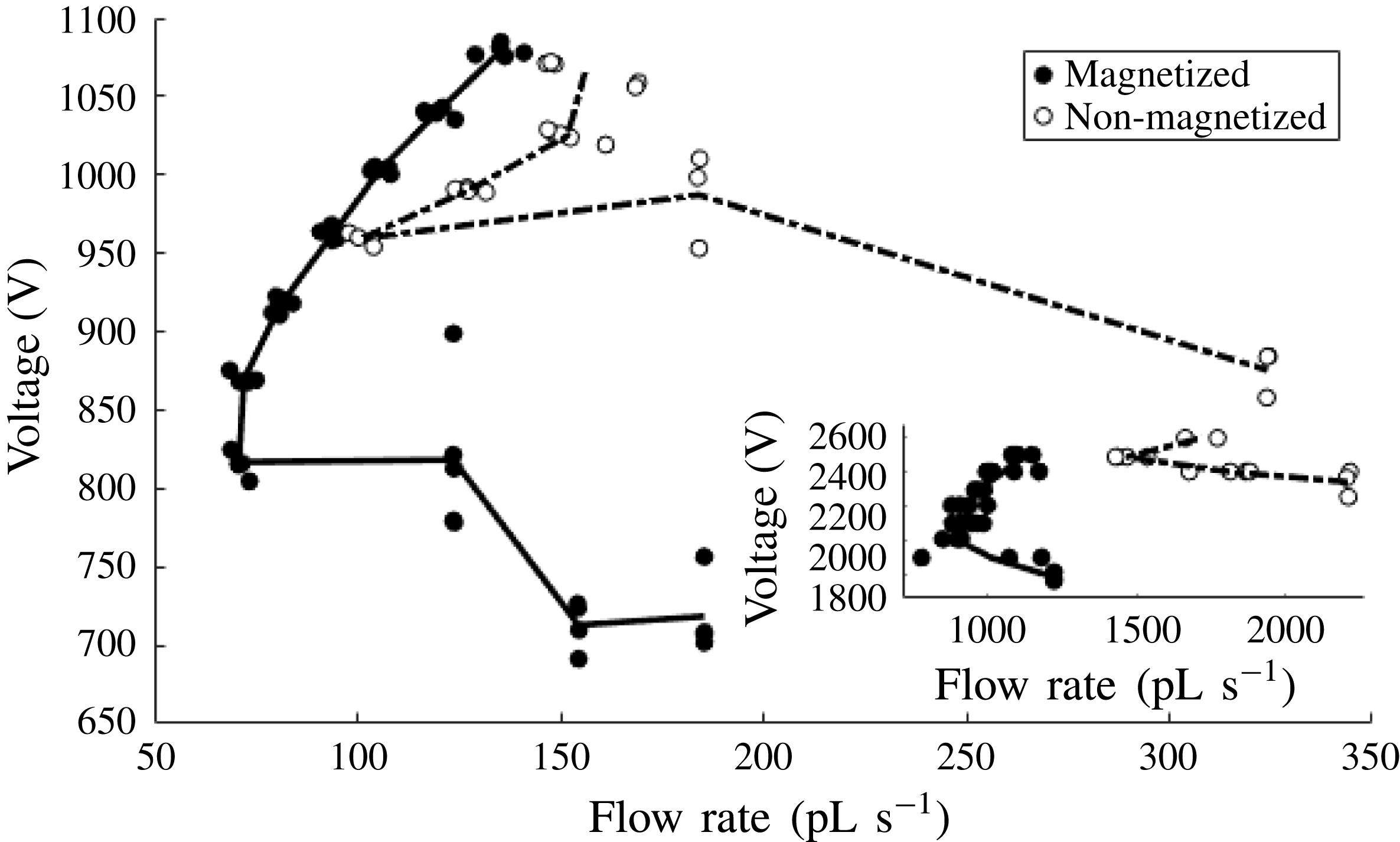
The second and far more relevant effect of magnetization clearly observable in figure 4 is that it widens substantially the range of stability towards smaller flow rates and currents. This behaviour may be appreciated even better in the stability islands depicted in figure 5, which are substantially shifted by magnetization towards the lower left. Voltages, currents, flow rates and corresponding standard deviations defining these boundaries are given in table form in the supplementary material. The global minimum flow rate found at any voltage is decreased by 30 % (from
 $101\pm 3.1$
to
 $71\pm 1.8~\text{pl}~\text{s}^{-1}$
) for the high conductivity liquid, and by 40 % (from
 $1469\pm 49.5$
to
 $894\pm 25.5~\text{pL}~\text{s}^{-1}$
) for the low conductivity liquid. Further, the onset voltage referring to the smallest voltage at which a Taylor cone forms was also reduced by 23 % (250 V) in the high conductivity liquid and 24 % (550 V) in the low conductivity liquid. In the high conductivity case, the lowest current observed in a stable magnetized cone was
 $102\pm 6.2~\text{nA}$
compared with a minimum current of
 $106\pm 3.5~\text{nA}$
in the non-magnetized cone. This result is observed at the moderate magnetic field of
 $23\,490~\text{A}~\text{m}^{-1}$
(300 Gauss), which produces 96.9 % of saturation magnetization in this ferrofluid.
Lower left corner of the Taylor cone stability island. The magnetized cone reaches substantially smaller flow rates and remains stable at lower voltages than its non-magnetized counterpart. The main figure is for the high conductivity liquid. The inset shows the lowest flow rate portion of the low conductivity liquid.

Notice in figure 5 two kinds of sequences of points, either horizontally or vertically aligned, corresponding respectively to excursions towards the stability boundary at either constant voltage or constant flow rate. Their dispersion provides a measure of the reproducibility of the position of this boundary, which is more variable for voltage (vertical) displacements at fixed
 $Q$
than for horizontal displacements.
Magnetized Taylor cones of sample A at
 $200~\text{pl}~\text{s}^{-1}$
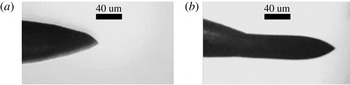
. (a) 1200 volts, (b) extended cone at 1000 volts.

Another unusual phenomenon inaccessible without a magnetic field was observed in magnetized cones at low voltages. At relatively high flow rates, the surprisingly long stable meniscus shown in figure 6 forms readily. A less extreme extended morphology is sometimes seen in non-magnetized sprays, but it is generally transient (periodic), with the meniscus volume slowly increasing and then abruptly decreasing via liquid detachment. There are two studies on more moderately extended acorn-shaped stable Taylor cones (Chen, Pui & Kaufman Reference Chen, Pui and Kaufman1995; Tang & Gomez Reference Tang and Gomez1995). Both are specific for electrospraying water into an atmosphere containing
 $\text{CO}_{2}$
, introduced to moderate the tendency for a corona discharge to form (due to the high voltages required in this high surface tension liquid). Both references reported a peculiar widening of the stability island towards reduced minimal flow rates. Tang and Gomez reported a tenfold reduction in minimal flow rate, resulting in average charge/volume ratios exceeding the maximum possible that could be produced if all the solution cations and none of the anions had been sprayed. This paradox suggested that part of the current was originating in the gas phase by a mild electrical discharge, a point that was confirmed by mass spectrometric analysis (Tang & Gomez Reference Tang and Gomez1995; Tang, Gomez & Fernandez de la Mora Reference Tang, Gomez and Fernandez de la Mora1999). Prior electrospraying regimes with long menisci and extended stability islands therefore belong to a special breed that is particularly difficult to reproduce. On the other hand, high elongations are a characteristic feature of stable ferrofluid drops in strong magnetic fields (Bacri & Salin Reference Bacri and Salin1982; Brancher & Zouaoui Reference Brancher and Zouaoui1987; Sero-Guillaume et al.
Reference Sero-Guillaume, Zouaoui, Bernardin and Brancher1992; Stone et al.
Reference Stone, Lister and Brenner1999; Lavrova et al.
Reference Lavrova, Matthies, Mitkova, Polevikov and Tobiska2006; Gollwitzer et al.
Reference Gollwitzer, Matthies, Richter, Rehberg and Tobiska2007). We conclude that the stability of this unusual meniscus is brought about by the applied axial magnetic field. Remarkably, the two rather different configurations shown in figure 6 result in almost identical emitted currents. As the flow rate is reduced or the voltage is increased, this extended cone retracts continuously and stably to the short standard cone.
4 Discussion
A first relevant practical question is how much drop size reduction may be achieved by magnetization. No direct drop size measurements were made. However, from the current and flow rate data collected from Taylor cones at the stability boundary shown in figure 5, we may extract the mean volume/charge ratio,
 $4\unicode[STIX]{x03C0}R^{3}/(3q)=Q/I$
. Further using the well-established fact that the average droplet is charged to a fair fraction
 $f_{R}$
of the Rayleigh limit:
 $q=f_{R}8\unicode[STIX]{x03C0}(\unicode[STIX]{x1D700}_{o}\unicode[STIX]{x1D6FE}R^{3})^{1/2}$
, results in
 $$\begin{eqnarray}R=(6^{2}f_{R}^{2}\unicode[STIX]{x1D6FE}\unicode[STIX]{x1D700}_{o}Q^{2}/I^{2})^{1/3}.\end{eqnarray}$$
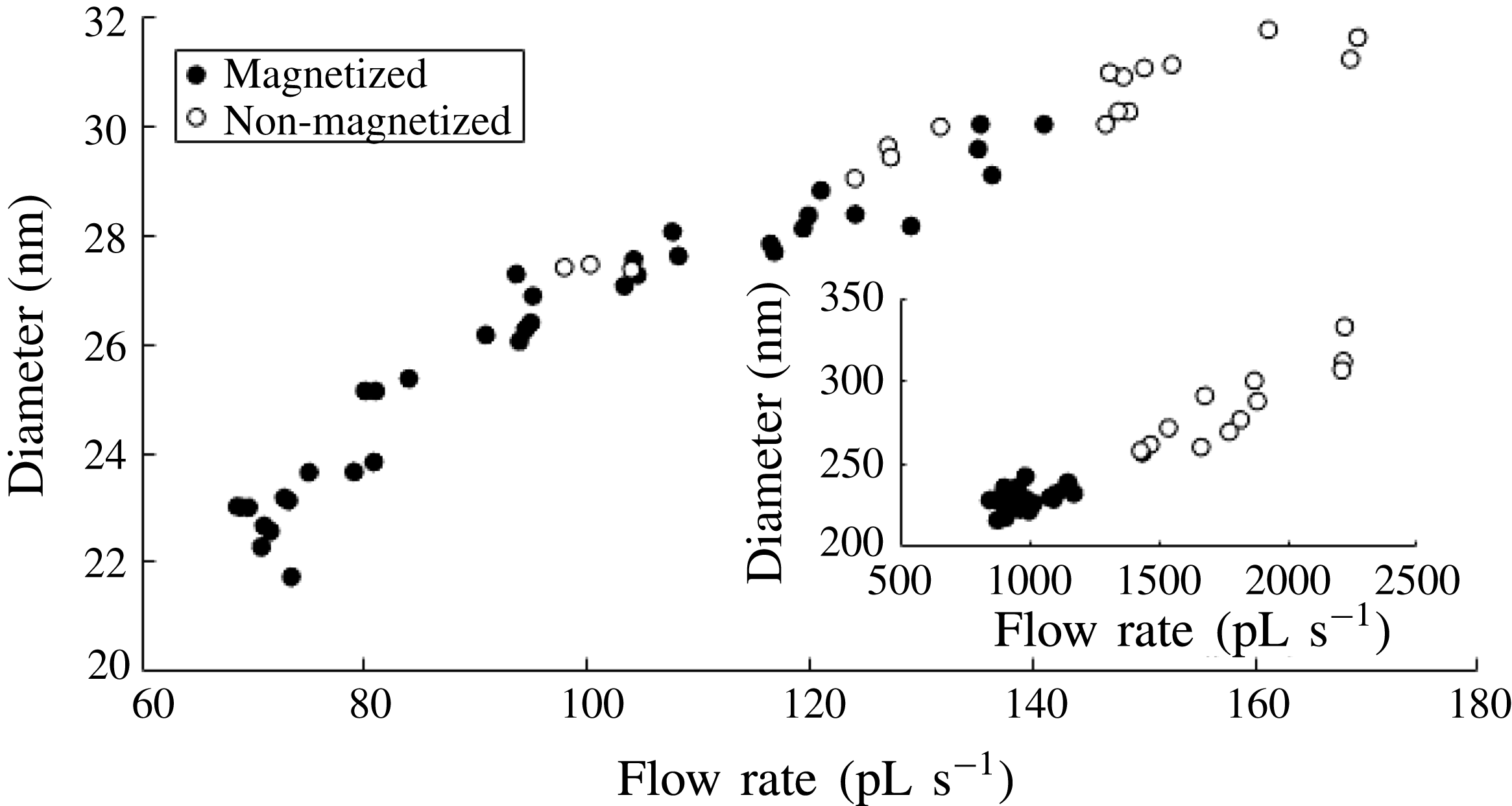
Corresponding approximate expected droplet diameter are collected in figure 7 based on the value
 $f_{R}=0.44$
proposed by Collins et al. (Reference Collins, Sambath, Harris and Basaran2013). The magnetic field decreases the minimum diameters by 20.7 % in sample A and 16.2 % in sample B.
Estimated diameters at the smallest flow rates at all tested voltages. Main figure: sample A. Inset: sample B.

Besides reducing the drop size, a reduced flow rate has been shown to narrow the drop size distribution (Rosell-Llompart & Fernández de la Mora Reference Rosell-Llompart and Fernández de la Mora1994). King (Reference King2014) has further theorized that magnetizing an electrified jet dampens the whipping breakup mode, which should also lead to a narrower size distribution over an unusually wide
 $Q$
range.
In a forthcoming study with ferrofluids with higher magnetization and a substantially lower electrical conductivity we observe a fourfold magnetic reduction in the minimal flow rate. There is accordingly an indubitable favourable effect of the magnetic fields on jet stability, which increases with the ratio of magnetic over electric stresses. However, the present observation of substantial magnetic stabilization even with minimal magnetic contribution to both the tip stress and the spray current is paradoxical. Understanding how such small magnetic fields modify the stability of purely electrified jets evidently requires first understanding the stability limits of the basic electric problem. Unfortunately relatively little is currently known about what limits the minimal flow rate in electrosprays. There is a clear limit to the
 $I/Q$
ratio achievable set by two simple features of the problem. When the capillary bringing the flow is metallic the electric field in its interior is null, so the electrolyte within the capillary carries no current. The metal can inject positive current into the meniscus, but only by neutralizing negative ions in the liquid. The largest charge that may be injected in a neutral liquid containing a fully dissociated salt at concentration
 $n$
is that neutralizing all negative incoming ions. Therefore
 $I_{max}=neQ$
, where
 $e$
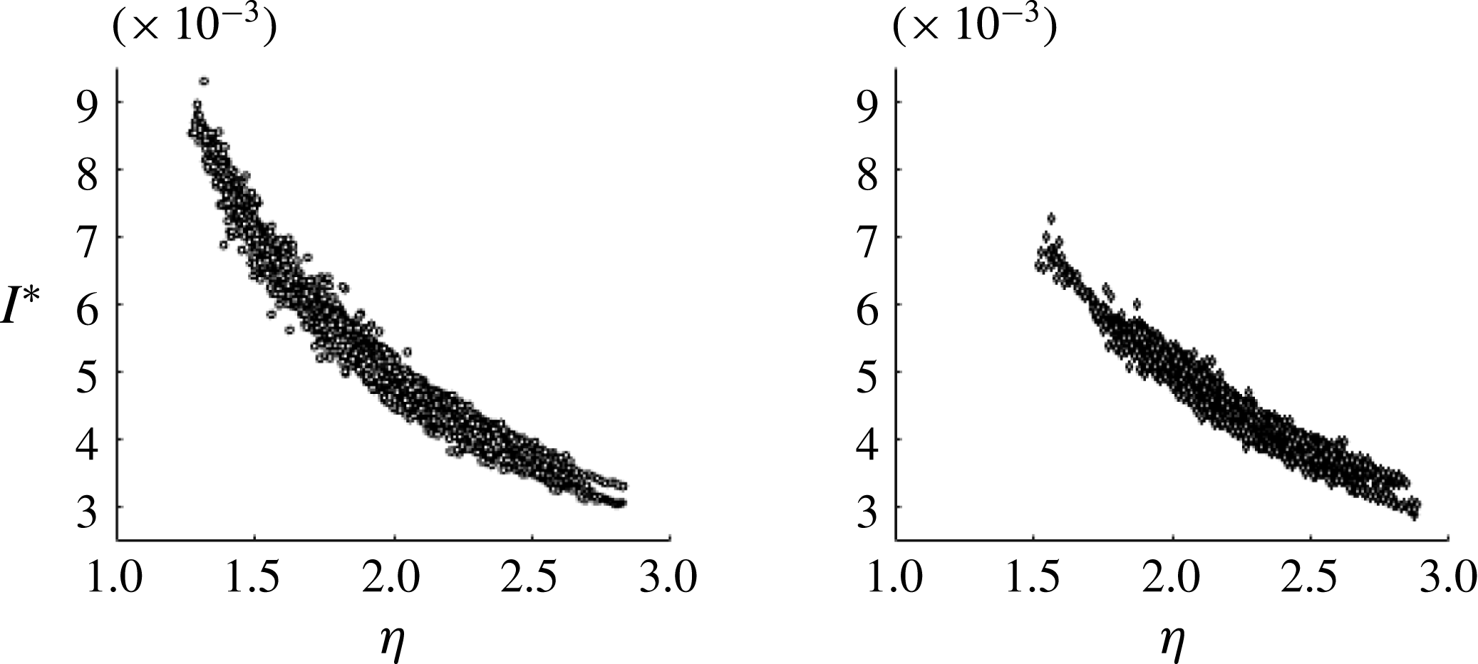
is the charge on each negative ion. This full neutralization limit is actually reached in exceptional cases involving very polar liquids of low viscosity such as water and formamide (Fernandez de la Mora & Loscertales Reference Fernandez de la Mora and Loscertales1994). That the full neutralization limit fails (by over two orders of magnitude) to explain the minimal flow rate of our sulfolane ferrofluid is clear from figure 8, representing the same data of figure 4 making the spray current dimensionless with
 $I_{max}$
:
 $$\begin{eqnarray}I^{\ast }=I/(neQ).\end{eqnarray}$$
Several studies have proposed on purely empirical grounds that the minimal flow rate is captured by a value of order one for the dimensionless variable (Fernandez de la Mora Reference Fernandez de la Mora2007)
 $$\begin{eqnarray}\unicode[STIX]{x1D702}=\sqrt{\frac{\unicode[STIX]{x1D70C}KQ}{\unicode[STIX]{x1D6FE}\unicode[STIX]{x1D716}_{o}}},\end{eqnarray}$$
where
 $\unicode[STIX]{x1D70C}$
is the liquid density. Figure 8 uses
 $\unicode[STIX]{x1D702}$
as the horizontal variable, showing that it does indeed take values of order one in stable electrospray operation. In figure 8 we see that the magnetized and non-magnetized samples A reach
 $\unicode[STIX]{x1D702}=1.30$
and 1.53, respectively (
 $\unicode[STIX]{x1D702}=0.78$
and 1.02 for sample B). These observations, however, are quite far from providing a satisfactory explanation for the limited stability range of either magnetized or non-magnetized sprays.

We conclude with remarks on ongoing and future theoretical analyses of the minimum flow rate in non-magnetized electrosprays. An article by Higuera (Reference Higuera2017) currently under review in this journal provides the first systematic effort towards such a theory, identifying two regimes, one of which includes the experimental parameter
 $\unicode[STIX]{x1D702}$
introduced in (4.3). An important point contributed by Gamero-Castaño (Reference Gamero-Castaño2010) but not yet widely used is that dissipation plays a central role in determining the structure of electrified cone jets. And indeed, if the energy equation accounting for electrical and viscous dissipation phenomena is written in quasi one-dimensional form for the electrified jet, the parameter
 $\unicode[STIX]{x1D702}$
is one of the two that appears naturally. The same two parameters arise also in the numerical study of Collins et al. (Reference Collins, Sambath, Harris and Basaran2013), even though the problem analysed is not steady but transient.
5 Conclusions
Taking advantage of a new ferrofluid developed at the University of Sydney having a wide range of electrical conductivities and very small volatility, we have studied the characteristics of Taylor cones of ferrofluids with and without uniform magnetic fields, with the following findings:
-
(i) In their shared region of stability, both magnetized and non-magnetized ferrofluids obey approximate
 $I\sim Q^{1/2}$
laws, both curves showing rather weak dependences on voltage.
-
(ii) Within that shared stability region, magnetization has minor effect on the current emitted at a given flow rate, even though it permits sizable reductions of the operating voltage.
-
(iii) The high curvature region of purely magnetic tips of ferrofluids turns out to be considerably less sharp than that of purely electrified conducting liquids, suggesting at first sight that adding a magnetic field would have little effect on the stability of electrified liquid cones. This impression, however, is falsified by experiments.
-
(iv) The range of flow rates, currents and voltages producing stable Taylor cones is considerably widened by the presence of magnetic fields, enabling in particular the production of smaller drops than attainable in conventional electrospraying.
-
(v) An additional manifestation of the ability of magnetic fields to stabilize an electrified meniscus is the discovery of stable elongated Taylor cones in the presence of magnetic fields, whose analogues in non-magnetized situations exist only in a transient form or in the presence of mild corona discharge in the gas surrounding the liquid meniscus.
-
(vi) A simple explanation for the magnetic stabilization observed hinges on the still pending rationalization for the minimal flow rate in purely electrified liquids.

Acknowledgements
This work was funded by AFOSR contract FA9550-14-1-0337 (Michigan Tech. subcontract) at Yale, and by the US Air Force Asian Office of Aerospace Research and Development at the University of Sydney. We thank Sirtex Medical for funding and for supplying the magnetic particles used. We are grateful to Professor F. Higuera (Polytechnic University of Madrid) for providing a persuasive explanation for the lack of strictly conical tips in real ferrofluids. Valuable discussions with Professor B. King (University of Michigan), L. J. Perez-Lorenzo (Yale) and J. Cubas (Polytechnic University of Madrid) are gratefully acknowledged.
Supplementary material
Supplementary material is available at https://doi.org/10.1017/jfm.2017.589.