1 Introduction
Concentrated suspensions of non-colloidal rigid particles present two main non-Newtonian rheological trends, namely finite normal stress differences under shear flow and transient effects (see, for example, the recent review by Guazzelli & Pouliquen (Reference Guazzelli and Pouliquen2018)). (i) Since the early work of Gadala-Maria (Reference Gadala-Maria1979), normal stress differences have been investigated in various flow geometries (Zarraga, Hill & Leighton Reference Zarraga, Hill and Leighton2000; Singh & Nott Reference Singh and Nott2003; Boyer, Pouliquen & Guazzelli Reference Boyer, Pouliquen and Guazzelli2011; Couturier et al. Reference Couturier, Boyer, Pouliquen and Guazzelli2011; Dai et al. Reference Dai, Bertevas, Qi and Tanner2013; Dbouk, Lobry & Lemaire Reference Dbouk, Lobry and Lemaire2013). These measurements consistently show that the second normal stress difference  $N_{2}$ is negative, with an absolute value that grows with volume fraction
 $\unicode[STIX]{x1D719}$. The first normal stress difference
 $N_{1}$ is generally found to be much smaller, in absolute value, than
 $|N_{2}|$. While most studies reported negative
 $N_{1}$ values, a few also reported positive values especially at high volume fractions. (ii) Using shear-reversal experiments, Gadala-Maria & Acrivos (Reference Gadala-Maria and Acrivos1980) showed that non-colloidal suspensions present transient rheological responses, characterized by a rate-independent evolution of the shear viscosity over typical strains of a few units, before this quantity eventually reaches its steady-state value. These shear-reversal experiments were later revisited by Kolli, Pollauf & Gadala-Maria (Reference Kolli, Pollauf and Gadala-Maria2002) and Blanc, Peters & Lemaire (Reference Blanc, Peters and Lemaire2011). All these authors related the transient effects to the development of microstructure anisotropy under shear flow, and attempted to quantify this anisotropy using the pair distribution function.
Most non-Newtonian trends of concentrated suspensions can be captured by particle-based numerical simulations, which offer additional insights into the physical processes at play. Earliest approaches were based on Stokesian dynamics, in which hydrodynamic interactions are split into far-field and near-field (lubrication) contributions (Brady & Bossis Reference Brady and Bossis1985). Numerous studies showed that essential ingredients to obtain realistic rheological behaviour in these simulations have to be added, in particular, the existence of finite normal stress differences, to account for particle contacts through short-range repulsive forces (Nott & Brady Reference Nott and Brady1994; Sierou & Brady Reference Sierou and Brady2002). Numerical results also demonstrated that frictional interactions should be taken into account to recover correct orders of magnitude for these normal stress differences, i.e.  $|N_{1}|<|N_{2}|$ (Sierou & Brady Reference Sierou and Brady2002; Mari et al. Reference Mari, Seto, Morris and Denn2014). Similar conclusions concerning the critical role of particle friction were reached by Gallier et al. (Reference Gallier, Lemaire, Peters and Lobry2014), using a more accurate direct numerical simulation method to model hydrodynamic interactions. More recently, Peters et al. (Reference Peters, Ghigliotti, Gallier, Blanc, Lemaire and Lobry2016) and Chacko et al. (Reference Chacko, Mari, Fielding and Cates2018) were also able to successfully simulate transient effects during shear reversal using direct numerical simulation and simplified Stokesian dynamics approaches, respectively. These particle-based simulations make it possible to continuously vary physical parameters and perform numerical experiments, thereby providing datasets that are well complementary to ‘real’ experiments. However, due to the high demand in computing power, they are still limited to small systems with a relatively low number of particles (a few thousand at most).
Unlike discrete particle-based models, continuous rheological models are suited to the simulation of large systems. However, the elaboration of constitutive laws able to reproduce both normal stress differences and transient features has proved to be a challenging task (e.g. Denn & Morris Reference Denn and Morris2014). General expressions for the bulk Cauchy stress tensor of suspensions can be obtained in the frame of two-phase mixture models (Jackson Reference Jackson2000; Nott, Guazzelli & Pouliquen Reference Nott, Guazzelli and Pouliquen2011; Baumgarten & Kamrin Reference Baumgarten and Kamrin2019), and involve contributions from both the interstitial fluid and the particles. For practical applications, physical closures need to be postulated for these different contributions. Nott & Brady (Reference Nott and Brady1994) introduced the suspension balance model (later extended by Morris & Boulay (Reference Morris and Boulay1999) and Miller & Morris (Reference Miller and Morris2006)), which involves explicit empirical expressions for the particle-induced normal stress components. This model provides relatively accurate predictions for steady-state flows and, when coupled to an evolution equation for the volume fraction  $\unicode[STIX]{x1D719}$ (that arises from mass and momentum conservation of the particle phase), can also account for particle migration processes. A similar type of approach based on explicit stress closures was recently followed by Singh et al. (Reference Singh, Mari, Denn and Morris2018), who proposed a model describing the transition to shear-thickening in highly concentrated suspensions. By construction, however, these models do not attempt to capture transient rheological effects.
Transient effects can be described by introducing a conformation tensor, denoted  $\boldsymbol{b}_{e}$ in this paper, which represents microstructure anisotropy. Note that conformation tensors are also sometimes referred to as texture tensors (see e.g. Lehoucq et al. Reference Lehoucq, Weiss, Dubrulle, Amon, le Bouil, Crassous, Amitrano and Graner2015). For non-colloidal suspensions, the conformation tensor
 $\boldsymbol{b}_{e}$ needs to obey an evolution equation that ensures rate-independence, i.e. this equation should have no characteristic time (e.g. Goddard Reference Goddard1982). Hand (Reference Hand1962) formulated general properties for anisotropic fluids, and expressed the Cauchy stress tensor
 $\unicode[STIX]{x1D748}$ as a function of both
 $\boldsymbol{b}_{e}$ and the strain rate tensor
 $\dot{\unicode[STIX]{x1D738}}$. Phan-Thien (Reference Phan-Thien1995) proposed a differential constitutive equation for the conformation tensor that led, for the first time, to predictions qualitatively in agreement with experimental observations during shear reversal. Goddard (Reference Goddard2006) revisited this approach, and proposed a model involving twelve material parameters and two tensors for describing the anisotropy. By a systematic fitting procedure on a limited dataset, he obtained numerical results in quantitative agreement with experiments for transient effects and normal stress differences. Stickel, Phillips & Powell (Reference Stickel, Phillips and Powell2006) proposed a simplified expression for the Cauchy stress tensor, which is linear in terms of both the strain rate and the conformation tensors (see also Stickel, Phillips & Powell Reference Stickel, Phillips and Powell2007; Yapici, Powell & Phillips Reference Yapici, Powell and Phillips2009). While this latter model involves 13 free parameters, it failed to provide quantitative comparisons with shear-reversal experiments: an unexpected sharp spike in both apparent viscosity and normal stress differences was obtained at the time of the reversal. Using a much simpler model, involving only four free parameters and a linear evolution evolution for the conformation tensor, Ozenda, Saramito & Chambon (Reference Ozenda, Saramito and Chambon2018) recently obtained a good quantitative agreement with the shear-reversal measurements of Blanc et al. (Reference Blanc, Peters and Lemaire2011) for a wide range of volume fraction
 $\unicode[STIX]{x1D719}$. Furthermore, at the microstructural scale, the model successfully reproduced both the pair distribution function and the depletion angles measured by Blanc et al. (Reference Blanc, Lemaire, Meunier and Peters2013). However, this simple model predicts unphysical normal stress differences.
The objective of this paper is to propose a continuous rheological model that provides quantitative predictions for both normal stress differences and transient effects, for dilute to concentrated suspensions. For that purpose, we revisit and extend the model proposed by Ozenda et al. (Reference Ozenda, Saramito and Chambon2018) based on the general expansion of Hand (Reference Hand1962). We limit consideration to rate-independent constitutive responses, i.e. to suspensions dominated by hydrodynamic (and possibly frictional) interactions. We also restrict attention to concentration ranges sufficiently below jamming, such that granular plasticity effects arising from sustained frictional contacts between particles (e.g. granular dilatancy; Pailha & Pouliquen (Reference Pailha and Pouliquen2009), Baumgarten & Kamrin (Reference Baumgarten and Kamrin2019)) do not come into play. In particular, our model does not include the shear-thinning and shear-thickening effects observed in more complex systems and/or close to jamming transition (see e.g. Royer, Blair & Hudson (Reference Royer, Blair and Hudson2016), Singh et al. (Reference Singh, Mari, Denn and Morris2018)). When compared with previous tensorial approaches (Phan-Thien Reference Phan-Thien1995; Goddard Reference Goddard2006; Stickel et al. Reference Stickel, Phillips and Powell2006), the present model involves only seven adjustable parameters, and compares well with experiments. Section 2 presents the rheological model. Section 3 is devoted to simple shear flows. The system of time-dependent equations is expanded for this case, and the stationary solution is explicitly exhibited. The dependence of the material parameters upon volume fraction  $\unicode[STIX]{x1D719}$ is investigated, based on asymptotic analyses in the dilute and highly concentrated limits. In § 4, model predictions are compared with a large number of experimental results regarding both transient effects and steady-state normal stresses. As the presented model involves seven dimensionless constants, a systematic sensitivity study is performed (§ 5). Finally, results are summarized and discussed in § 6.
2 Mathematical model
2.1 Problem statement
Following Ozenda et al. (Reference Ozenda, Saramito and Chambon2018), let us introduce the conformation tensor  $\boldsymbol{b}_{e}=d_{0}^{-2}\langle \boldsymbol{\ell }\otimes \boldsymbol{\ell }\rangle$, where
 $\boldsymbol{\ell }$ is the branch vector joining the centres of two neighbouring particles and
 $d_{0}$ is the average distance between neighbouring particle centres in an isotropic configuration at rest. In the isotropic configuration at rest, we have
 $\boldsymbol{b}_{e}=\unicode[STIX]{x1D644}$, where
 $\unicode[STIX]{x1D644}$ is the identity matrix. For convenience, we introduce the tensor
 $\unicode[STIX]{x1D738}_{e}=c_{0}(\boldsymbol{b}_{e}-\unicode[STIX]{x1D644})$, where
 $c_{0}$ is a dimensionless constant that will be chosen later. The tensor
 $\unicode[STIX]{x1D738}_{e}$ is interpreted as the deformation of the microstructure with respect to rest configuration. As in Ozenda et al. (Reference Ozenda, Saramito and Chambon2018), we assume a linear evolution for
 $\unicode[STIX]{x1D738}_{e}$:
 $$\begin{eqnarray}\displaystyle & \displaystyle {\displaystyle \frac{\mathscr{D}_{a}\unicode[STIX]{x1D738}_{e}}{\mathscr{D}t}}+\unicode[STIX]{x1D6FF}_{1}|\dot{\unicode[STIX]{x1D738}}|\unicode[STIX]{x1D738}_{e}-\dot{\unicode[STIX]{x1D738}}=0, & \displaystyle\end{eqnarray}$$
 $$\begin{eqnarray}\displaystyle & \displaystyle \dot{\unicode[STIX]{x1D738}}=\unicode[STIX]{x1D735}\boldsymbol{u}+\unicode[STIX]{x1D735}\boldsymbol{u}^{\text{T}}, & \displaystyle\end{eqnarray}$$
where  $\dot{\unicode[STIX]{x1D738}}$ is the strain rate tensor,
 $\boldsymbol{u}$ is the velocity field of the suspension and
 $\unicode[STIX]{x1D6FF}_{1}$ is a positive dimensionless material parameter. The matrix norm
 $|\unicode[STIX]{x1D743}|$ is defined as
 $|\unicode[STIX]{x1D743}|^{2}=(\unicode[STIX]{x1D743}\boldsymbol{ : }\unicode[STIX]{x1D743})/2$ for any matrix
 $\unicode[STIX]{x1D743}$, with
 $(\cdot \!:\!\cdot )$ denoting the double contracted matrix product. We use in (2.1a) a general Gordon–Schowalter tensor derivative (Gordon & Schowalter Reference Gordon and Schowalter1972; Saramito Reference Saramito2016):
 $$\begin{eqnarray}{\displaystyle \frac{\mathscr{D}_{a}\unicode[STIX]{x1D738}_{e}}{\mathscr{D}t}}={\displaystyle \frac{\unicode[STIX]{x2202}\unicode[STIX]{x1D738}_{e}}{\unicode[STIX]{x2202}t}}+(\boldsymbol{u}\boldsymbol{\cdot }\unicode[STIX]{x1D735})\unicode[STIX]{x1D738}_{e}-W(\boldsymbol{u})\unicode[STIX]{x1D738}_{e}+\unicode[STIX]{x1D738}_{e}W(\boldsymbol{u})-{\displaystyle \frac{a}{2}}(\dot{\unicode[STIX]{x1D738}}\unicode[STIX]{x1D738}_{e}+\unicode[STIX]{x1D738}_{e}\dot{\unicode[STIX]{x1D738}}),\end{eqnarray}$$
where  $W(\boldsymbol{u})=(\unicode[STIX]{x1D735}\boldsymbol{u}-\unicode[STIX]{x1D735}\boldsymbol{u}^{\text{T}})/2$ and
 $a\in \,[-1,1]$. Note that Ozenda et al. (Reference Ozenda, Saramito and Chambon2018) used an upper-convected derivative, corresponding to
 $a=1$. Equation (2.1a) has no characteristic time, such that its solutions are rate-independent: in simple shear, changing the amplitude of the strain rate
 $\dot{\unicode[STIX]{x1D738}}$ leaves the evolution of
 $\dot{\unicode[STIX]{x1D738}}_{e}$ unchanged when expressed in terms of the dimensionless time
 $|\dot{\unicode[STIX]{x1D738}}|t$ (that is interpreted as a strain).
The Cauchy stress tensor  $\unicode[STIX]{x1D748}$ of the suspension is assumed to express as an analytical function of the two tensorial variables
 $\dot{\unicode[STIX]{x1D738}}$ and
 $\unicode[STIX]{x1D738}_{e}$. Following Hand (Reference Hand1962), and by virtue of the Cayley–Hamilton theorem, only the zeroth, first and second powers of
 $\dot{\unicode[STIX]{x1D738}}$ and
 $\unicode[STIX]{x1D738}_{e}$ can contribute to the expression. Furthermore, to preserve rate-independence, terms in
 $\dot{\unicode[STIX]{x1D738}}^{2}$ should also be discarded. After extensive tests to assess the effects of the various possible terms, we chose to consider the following expression for the Cauchy stress tensor:
 $$\begin{eqnarray}\unicode[STIX]{x1D748}=-p_{b}\unicode[STIX]{x1D644}+\unicode[STIX]{x1D702}\dot{\unicode[STIX]{x1D738}}+\unicode[STIX]{x1D702}_{e}\left\{\unicode[STIX]{x1D6FF}_{1}|\dot{\unicode[STIX]{x1D738}}|\unicode[STIX]{x1D738}_{e}+\unicode[STIX]{x1D6FD}\left({\displaystyle \frac{\unicode[STIX]{x1D738}_{e}^{2}\dot{\unicode[STIX]{x1D738}}+\dot{\unicode[STIX]{x1D738}}\unicode[STIX]{x1D738}_{e}^{2}}{2}}-|\dot{\unicode[STIX]{x1D738}}|\unicode[STIX]{x1D738}_{e}^{2}\right)+\unicode[STIX]{x1D6FF}_{2}\left({\displaystyle \frac{\unicode[STIX]{x1D738}_{e}\dot{\unicode[STIX]{x1D738}}+\dot{\unicode[STIX]{x1D738}}\unicode[STIX]{x1D738}_{e}}{2}}\right)\right\},\end{eqnarray}$$
where  $p_{b}$ is the bulk pressure of the suspension,
 $\unicode[STIX]{x1D702}$ and
 $\unicode[STIX]{x1D702}_{e}$ are characteristic viscosities and
 $\unicode[STIX]{x1D6FD}$ and
 $\unicode[STIX]{x1D6FF}_{2}$ are additional dimensionless material parameters. Note that the terms in the factors
 $\unicode[STIX]{x1D6FF}_{1}$ and
 $\unicode[STIX]{x1D6FF}_{2}$ are linear in
 $\unicode[STIX]{x1D738}_{e}$, while the term in the factor
 $\unicode[STIX]{x1D6FD}$ is quadratic in
 $\unicode[STIX]{x1D738}_{e}$. The present model represents an upgrade of that presented by Ozenda et al. (Reference Ozenda, Saramito and Chambon2018), which involved only one linear term and one nonlinear term. For the sake of simplicity and of formulating a minimal model, the scalar coefficients
 $\unicode[STIX]{x1D702}$,
 $\unicode[STIX]{x1D702}_{e}\unicode[STIX]{x1D6FD}$,
 $\unicode[STIX]{x1D702}_{e}\unicode[STIX]{x1D6FF}_{1}$ and
 $\unicode[STIX]{x1D702}_{e}\unicode[STIX]{x1D6FF}_{2}$ are assumed to be independent of the invariants of
 $\unicode[STIX]{x1D738}_{e}$, which is a restriction compared to the general theory of Hand (Reference Hand1962).
Constitutive equations (2.1) are coupled with mass and momentum conservations to obtain a closed problem for three unknowns, namely the suspension pressure  $p_{b}$, the suspension velocity
 $\boldsymbol{u}$ and the tensor describing the anisotropy of the microstructure
 $\unicode[STIX]{x1D738}_{e}$:
 $$\begin{eqnarray}\displaystyle \displaystyle {\displaystyle \frac{\mathscr{D}_{a}\unicode[STIX]{x1D738}_{e}}{\mathscr{D}t}}+\unicode[STIX]{x1D6FF}_{1}|\dot{\unicode[STIX]{x1D738}}|\unicode[STIX]{x1D738}_{e}-\dot{\unicode[STIX]{x1D738}} & = & \displaystyle 0,\end{eqnarray}$$
 $$\begin{eqnarray}\displaystyle \displaystyle \unicode[STIX]{x1D70C}\left({\displaystyle \frac{\unicode[STIX]{x2202}\boldsymbol{u}}{\unicode[STIX]{x2202}t}}+(\boldsymbol{u}\boldsymbol{\cdot }\unicode[STIX]{x1D735})\boldsymbol{u}\right)-\text{}\text{div}\,\unicode[STIX]{x1D748} & = & \displaystyle 0,\end{eqnarray}$$
 $$\begin{eqnarray}\displaystyle \displaystyle \text{div}\,\boldsymbol{u} & = & \displaystyle 0,\end{eqnarray}$$
 $\unicode[STIX]{x1D748}$ is expressed by (2.1c) and the strain rate tensor
 $\dot{\unicode[STIX]{x1D738}}$ is expressed by (2.1b). Note that
 $p_{b}$ in (2.1c) should be regarded as a Lagrange multiplier associated with the incompressibility constraint (2.2c). This set of equations is closed by appropriate boundary and initial conditions for
 $\boldsymbol{u}$ and
 $\unicode[STIX]{x1D738}_{e}$.
From (2.2a), we remark that the conformation tensor  $\boldsymbol{b}_{e}=c_{0}^{-1}(c_{0}\unicode[STIX]{x1D644}+\unicode[STIX]{x1D738}_{e})$ satisfies
 $$\begin{eqnarray}\displaystyle {\displaystyle \frac{\mathscr{D}_{a}\boldsymbol{b}_{e}}{\mathscr{D}t}}-c_{0}\unicode[STIX]{x1D6FF}_{1}|\dot{\unicode[STIX]{x1D738}}|\unicode[STIX]{x1D644}+c_{0}\unicode[STIX]{x1D6FF}_{1}|\dot{\unicode[STIX]{x1D738}}|\boldsymbol{b}_{e}=(1-ac_{0})\dot{\unicode[STIX]{x1D738}}. & & \displaystyle \nonumber\end{eqnarray}$$
Hence, by choosing the dimensionless constant  $c_{0}=1/a$, the right-hand side in the previous relation is zero. In the following, we also assume
 $a\in \! ]0,1\!]$. According to Hulsen (Reference Hulsen1990), and since
 $\unicode[STIX]{x1D6FF}_{1}>0$, these choices guarantee that the conformation tensor
 $\boldsymbol{b}_{e}$ is positive definite at any time, if this property is satisfied at initial time.
3 Simple shear and shear reversal
3.1 The reduced problem
Let us consider a simple shear flow with uniform shear rate. The  $x$ axis is in the flow direction and the
 $y$ axis is in the direction of velocity gradient, such that
 $\boldsymbol{u}(t,x,y,z)=(u_{x}(t,y),0,0)$. Let us denote
 $\dot{\unicode[STIX]{x1D6FE}}=\unicode[STIX]{x2202}_{y}u_{x}$ the uniform scalar shear rate, such that
 $|\dot{\unicode[STIX]{x1D6FE}}|=|\dot{\unicode[STIX]{x1D738}}|$. Evolution equation (2.2a) for
 $\unicode[STIX]{x1D738}_{e}(t)$ then reduces to the following system of ordinary differential equations:
 $$\begin{eqnarray}\displaystyle \displaystyle \unicode[STIX]{x2202}_{t}\unicode[STIX]{x1D6FE}_{e,xx}-(1\!+\!a)\dot{\unicode[STIX]{x1D6FE}}\,\unicode[STIX]{x1D6FE}_{e,xy}+\unicode[STIX]{x1D6FF}_{1}|\dot{\unicode[STIX]{x1D6FE}}|\,\unicode[STIX]{x1D6FE}_{e,xx} & = & \displaystyle 0,\end{eqnarray}$$
 $$\begin{eqnarray}\displaystyle \displaystyle \unicode[STIX]{x2202}_{t}\unicode[STIX]{x1D6FE}_{e,yy}+(1\!-\!a)\dot{\unicode[STIX]{x1D6FE}}\,\unicode[STIX]{x1D6FE}_{e,xy}+\unicode[STIX]{x1D6FF}_{1}|\dot{\unicode[STIX]{x1D6FE}}|\,\unicode[STIX]{x1D6FE}_{e,yy} & = & \displaystyle 0,\end{eqnarray}$$
 $$\begin{eqnarray}\displaystyle \displaystyle \unicode[STIX]{x2202}_{t}\unicode[STIX]{x1D6FE}_{e,xy}-{\displaystyle \frac{1\!+\!a}{2}}\dot{\unicode[STIX]{x1D6FE}}\,\unicode[STIX]{x1D6FE}_{e,yy}-{\displaystyle \frac{1\!-\!a}{2}}\dot{\unicode[STIX]{x1D6FE}}\,\unicode[STIX]{x1D6FE}_{e,xx}+\unicode[STIX]{x1D6FF}_{1}|\dot{\unicode[STIX]{x1D6FE}}|\,\unicode[STIX]{x1D6FE}_{e,xy} & = & \displaystyle \dot{\unicode[STIX]{x1D6FE}},\end{eqnarray}$$
 $$\begin{eqnarray}\displaystyle \displaystyle \unicode[STIX]{x2202}_{t}\unicode[STIX]{x1D6FE}_{e,xz}-(1\!+\!a)\dot{\unicode[STIX]{x1D6FE}}\,\unicode[STIX]{x1D6FE}_{e,yz}+\unicode[STIX]{x1D6FF}_{1}|\dot{\unicode[STIX]{x1D6FE}}|\,\unicode[STIX]{x1D6FE}_{e,xz} & = & \displaystyle 0,\end{eqnarray}$$
 $$\begin{eqnarray}\displaystyle \displaystyle \unicode[STIX]{x2202}_{t}\unicode[STIX]{x1D6FE}_{e,yz}+(1\!-\!a)\dot{\unicode[STIX]{x1D6FE}}\,\unicode[STIX]{x1D6FE}_{e,xz}+\unicode[STIX]{x1D6FF}_{1}|\dot{\unicode[STIX]{x1D6FE}}|\,\unicode[STIX]{x1D6FE}_{e,yz} & = & \displaystyle 0,\end{eqnarray}$$
 $$\begin{eqnarray}\displaystyle \displaystyle \unicode[STIX]{x2202}_{t}\unicode[STIX]{x1D6FE}_{e,zz}+\unicode[STIX]{x1D6FF}_{1}|\dot{\unicode[STIX]{x1D6FE}}|\,\unicode[STIX]{x1D6FE}_{e,zz} & = & \displaystyle 0.\end{eqnarray}$$
 $\unicode[STIX]{x1D6FE}_{e,xz}=\unicode[STIX]{x1D6FE}_{e,yz}=\unicode[STIX]{x1D6FE}_{e,zz}=0$ at
 $t=0$, such that these components remain zero at any time. The constitutive equation (2.1c) for
 $\unicode[STIX]{x1D748}$ becomes
 $$\begin{eqnarray}\displaystyle \hspace{-26.39996pt}\displaystyle \unicode[STIX]{x1D70E}_{xx} & = & \displaystyle -p_{b}+\unicode[STIX]{x1D702}_{e}\{\unicode[STIX]{x1D6FF}_{1}|\dot{\unicode[STIX]{x1D6FE}}|\unicode[STIX]{x1D6FE}_{e,xx}+\unicode[STIX]{x1D6FD}(\dot{\unicode[STIX]{x1D6FE}}(\unicode[STIX]{x1D6FE}_{e,xx}+\unicode[STIX]{x1D6FE}_{e,yy})\unicode[STIX]{x1D6FE}_{e,xy}-|\dot{\unicode[STIX]{x1D6FE}}|(\unicode[STIX]{x1D6FE}_{e,xx}^{2}+\unicode[STIX]{x1D6FE}_{e,xy}^{2}))+\unicode[STIX]{x1D6FF}_{2}\dot{\unicode[STIX]{x1D6FE}}\unicode[STIX]{x1D6FE}_{e,xy}\},\end{eqnarray}$$
 $$\begin{eqnarray}\displaystyle \hspace{-26.39996pt}\displaystyle \unicode[STIX]{x1D70E}_{yy} & = & \displaystyle -p_{b}+\unicode[STIX]{x1D702}_{e}\{\unicode[STIX]{x1D6FF}_{1}|\dot{\unicode[STIX]{x1D6FE}}|\unicode[STIX]{x1D6FE}_{e,yy}+\unicode[STIX]{x1D6FD}(\dot{\unicode[STIX]{x1D6FE}}(\unicode[STIX]{x1D6FE}_{e,xx}+\unicode[STIX]{x1D6FE}_{e,yy})\unicode[STIX]{x1D6FE}_{e,xy}-|\dot{\unicode[STIX]{x1D6FE}}|(\unicode[STIX]{x1D6FE}_{e,xy}^{2}+\unicode[STIX]{x1D6FE}_{e,yy}^{2}))+\unicode[STIX]{x1D6FF}_{2}\dot{\unicode[STIX]{x1D6FE}}\unicode[STIX]{x1D6FE}_{e,xy}\},\end{eqnarray}$$
 $$\begin{eqnarray}\displaystyle \hspace{-26.39996pt}\displaystyle \unicode[STIX]{x1D70E}_{zz} & = & \displaystyle -p_{b},\end{eqnarray}$$
 $$\begin{eqnarray}\displaystyle \hspace{-24.0pt}\unicode[STIX]{x1D70E}_{xy} & = & \displaystyle \unicode[STIX]{x1D702}\dot{\unicode[STIX]{x1D6FE}}+\unicode[STIX]{x1D702}_{e}\left\{\unicode[STIX]{x1D6FF}_{1}|\dot{\unicode[STIX]{x1D6FE}}|\unicode[STIX]{x1D6FE}_{e,xy}+\unicode[STIX]{x1D6FD}\left({\displaystyle \frac{\dot{\unicode[STIX]{x1D6FE}}}{2}}(\unicode[STIX]{x1D6FE}_{e,xx}^{2}+\unicode[STIX]{x1D6FE}_{e,yy}^{2}+2\unicode[STIX]{x1D6FE}_{e,xy}^{2})-|\dot{\unicode[STIX]{x1D6FE}}|(\unicode[STIX]{x1D6FE}_{e,xx}+\unicode[STIX]{x1D6FE}_{e,yy})\unicode[STIX]{x1D6FE}_{e,xy}\right)\right.\nonumber\\ \displaystyle \hspace{-24.0pt} & & \displaystyle \left.+\,{\displaystyle \frac{\unicode[STIX]{x1D6FF}_{2}\dot{\unicode[STIX]{x1D6FE}}}{2}}(\unicode[STIX]{x1D6FE}_{e,xx}+\unicode[STIX]{x1D6FE}_{e,yy})\right\},\end{eqnarray}$$
 $$\begin{eqnarray}\displaystyle \hspace{-24.0pt}\unicode[STIX]{x1D70E}_{xz} & = & \displaystyle \unicode[STIX]{x1D70E}_{yz}=0.\end{eqnarray}$$
 $\dot{\unicode[STIX]{x1D6FE}}$ is given. Explicit expressions of the stress components are then obtained from (3.2). In the following, we will also consider situations in which the shear stress
 $\unicode[STIX]{x1D70E}_{xy}$ is imposed. In this case, numerical solutions of the coupled equations (3.1)–(3.2) are computed using lsode ordinary differential equation solver (Radhakrishnan & Hindmarsh Reference Radhakrishnan and Hindmarsh1993) implemented within the numpy-scipy environment (Virtanen et al. Reference Virtanen, Gommers, Oliphant, Haberland, Reddy, Cournapeau, Burovski, Peterson, Weckesser and Bright2020).
JonOliPet-2001.
3.2 Explicit solution in steady state
The steady-state solution of (3.1a) to (3.1c) is written as
 $$\begin{eqnarray}\displaystyle & \displaystyle \unicode[STIX]{x1D6FE}_{e,xx}={\displaystyle \frac{1+a}{1-a^{2}+\unicode[STIX]{x1D6FF}_{1}^{2}}}, & \displaystyle\end{eqnarray}$$
 $$\begin{eqnarray}\displaystyle & \displaystyle \unicode[STIX]{x1D6FE}_{e,yy}={\displaystyle \frac{-(1-a)}{1-a^{2}+\unicode[STIX]{x1D6FF}_{1}^{2}}}, & \displaystyle\end{eqnarray}$$
 $$\begin{eqnarray}\displaystyle & \displaystyle \unicode[STIX]{x1D6FE}_{e,xy}={\displaystyle \frac{\unicode[STIX]{x1D6FF}_{1}\,\text{sgn}(\dot{\unicode[STIX]{x1D6FE}})}{1-a^{2}+\unicode[STIX]{x1D6FF}_{1}^{2}}}. & \displaystyle\end{eqnarray}$$
 $\unicode[STIX]{x1D702}_{app}=\unicode[STIX]{x1D70E}_{xy}/\dot{\unicode[STIX]{x1D6FE}}$ and normal stress differences
 $N_{1}=\unicode[STIX]{x1D70E}_{xx}-\unicode[STIX]{x1D70E}_{yy}$ and
 $N_{2}=\unicode[STIX]{x1D70E}_{yy}-\unicode[STIX]{x1D70E}_{zz}$ are then easily deduced from (3.2a)–(3.2d):
 $$\begin{eqnarray}\displaystyle \displaystyle \unicode[STIX]{x1D702}_{app} & = & \displaystyle \unicode[STIX]{x1D702}+{\displaystyle \frac{\unicode[STIX]{x1D702}_{e}}{1-a^{2}+\unicode[STIX]{x1D6FF}_{1}^{2}}}\left(\unicode[STIX]{x1D6FF}_{1}^{2}+a\unicode[STIX]{x1D6FF}_{2}+{\displaystyle \frac{((1+a^{2}+\unicode[STIX]{x1D6FF}_{1}^{2})-2a\unicode[STIX]{x1D6FF}_{1})\unicode[STIX]{x1D6FD}}{1-a^{2}+\unicode[STIX]{x1D6FF}_{1}^{2}}}\right),\end{eqnarray}$$
 $$\begin{eqnarray}\displaystyle \displaystyle N_{1} & = & \displaystyle {\displaystyle \frac{2\unicode[STIX]{x1D702}_{e}|\dot{\unicode[STIX]{x1D6FE}}|}{1-a^{2}+\unicode[STIX]{x1D6FF}_{1}^{2}}}\left(\unicode[STIX]{x1D6FF}_{1}-{\displaystyle \frac{2a\unicode[STIX]{x1D6FD}}{1-a^{2}+\unicode[STIX]{x1D6FF}_{1}^{2}}}\right),\end{eqnarray}$$
 $$\begin{eqnarray}\displaystyle \displaystyle N_{2} & = & \displaystyle {\displaystyle \frac{\unicode[STIX]{x1D702}_{e}|\dot{\unicode[STIX]{x1D6FE}}|}{1-a^{2}+\unicode[STIX]{x1D6FF}_{1}^{2}}}\left(\unicode[STIX]{x1D6FF}_{1}(-1+a+\unicode[STIX]{x1D6FF}_{2})+{\displaystyle \frac{(2a\unicode[STIX]{x1D6FF}_{1}-((1\!-\!a)^{2}+\unicode[STIX]{x1D6FF}_{1}^{2}))\unicode[STIX]{x1D6FD}}{1-a^{2}+\unicode[STIX]{x1D6FF}_{1}^{2}}}\right).\end{eqnarray}$$
We also define the particle pressure  $p_{p}=p-p_{b}$, where
 $p=-\text{tr}(\unicode[STIX]{x1D748})/3$ is the total pressure of the suspension. In steady state
 $$\begin{eqnarray}\displaystyle & \displaystyle p_{p}=-{\displaystyle \frac{2\unicode[STIX]{x1D702}_{e}|\dot{\unicode[STIX]{x1D6FE}}|}{3(1-a^{2}+\unicode[STIX]{x1D6FF}_{1}^{2})}}\left(\unicode[STIX]{x1D6FF}_{1}(a+\unicode[STIX]{x1D6FF}_{2})+{\displaystyle \frac{(2a\unicode[STIX]{x1D6FF}_{1}-(1+a^{2}+\unicode[STIX]{x1D6FF}_{1}^{2}))\unicode[STIX]{x1D6FD}}{1-a^{2}+\unicode[STIX]{x1D6FF}_{1}^{2}}}\right). & \displaystyle\end{eqnarray}$$
3.3 Dependence of material parameters upon volume fraction
The rheological model presented in § 2 involves six material parameters: two viscosities  $\unicode[STIX]{x1D702}$ and
 $\unicode[STIX]{x1D702}_{e}$ and four dimensionless parameters
 $a$,
 $\unicode[STIX]{x1D6FF}_{1}$,
 $\unicode[STIX]{x1D6FF}_{2}$ and
 $\unicode[STIX]{x1D6FD}$. Preliminary tests to fit experimental data for different volume fractions
 $\unicode[STIX]{x1D719}$ (see § 4) showed that all these parameters, except
 $a$, have to vary with
 $\unicode[STIX]{x1D719}$. Following these preliminary investigations, we assumed
 $a$ to be independent of
 $\unicode[STIX]{x1D719}$, and the five remaining parameters to depend only upon the reduced volume fraction
 $\unicode[STIX]{x1D713}=\unicode[STIX]{x1D719}/\unicode[STIX]{x1D719}_{m}$, with
 $\unicode[STIX]{x1D719}_{m}$ the maximal volume fraction of the suspension. This latter assumption is required to obtain a model that can be applied to different experimental datasets characterized by different values of
 $\unicode[STIX]{x1D719}_{m}$. In practice,
 $\unicode[STIX]{x1D719}_{m}$ can vary between
 $0.53$ and
 $0.64$, typically depending on particle shape, particle roughness, etc. (e.g. Guazzelli & Pouliquen Reference Guazzelli and Pouliquen2018).
As shown in appendix A, the parameter  $\unicode[STIX]{x1D6FF}_{1}$ is directly related to the depletion angle
 $\unicode[STIX]{x1D703}_{e}$, i.e. the angle between the
 $x$ axis and the direction of the eigenvector associated to the largest eigenvalue of
 $\unicode[STIX]{x1D738}_{e}$:
 $\unicode[STIX]{x1D6FF}_{1}=\tan (2\unicode[STIX]{x1D703}_{e})$. Based on the experimental measurements of
 $\unicode[STIX]{x1D703}_{e}$ provided by Blanc et al. (Reference Blanc, Lemaire, Meunier and Peters2013), the following dependence law is proposed for
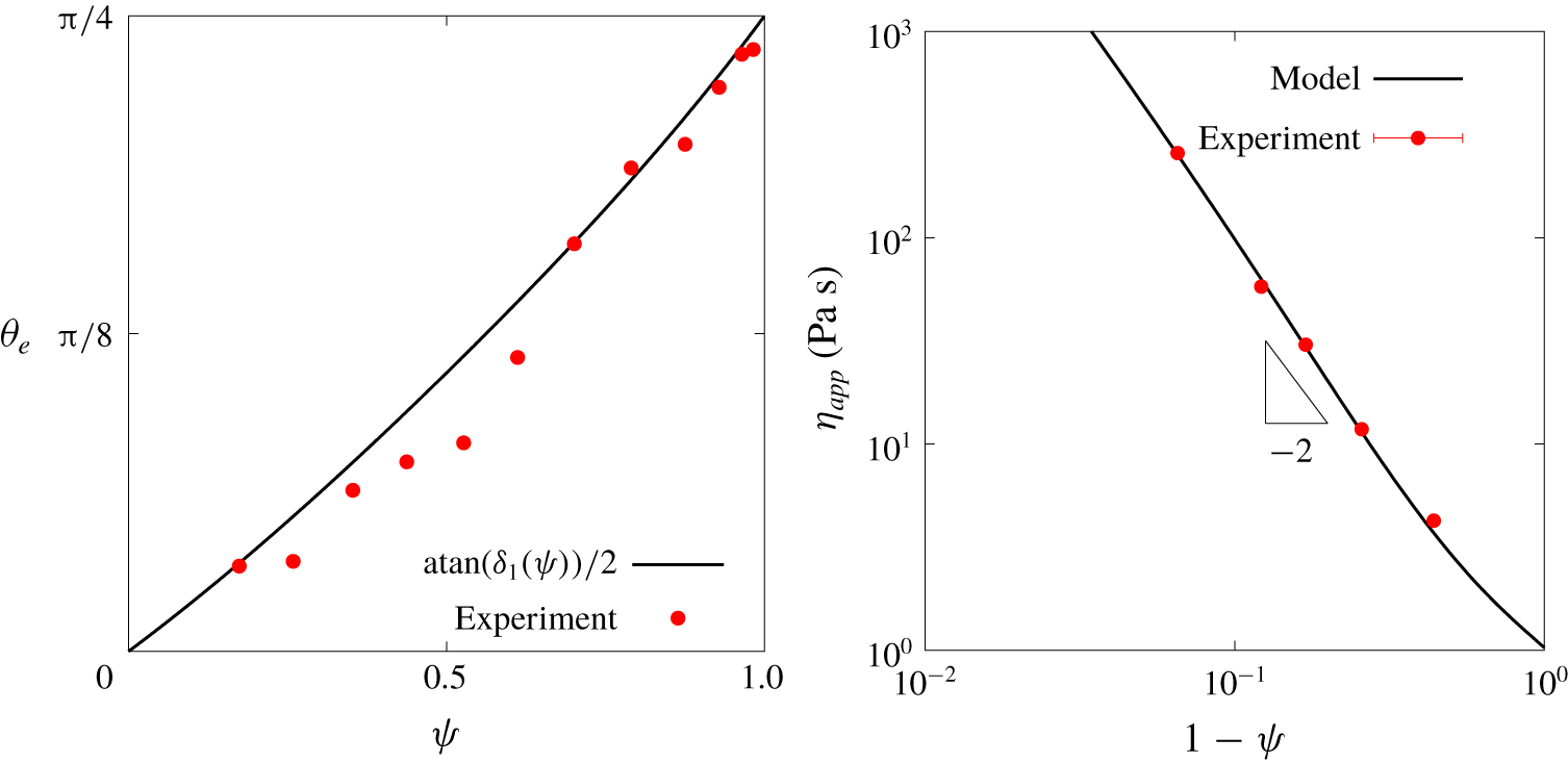
 $\unicode[STIX]{x1D6FF}_{1}$ (see figure 1):
 $$\begin{eqnarray}\unicode[STIX]{x1D6FF}_{1}(\unicode[STIX]{x1D713})=\bar{\unicode[STIX]{x1D6FF}}_{1}((1-\unicode[STIX]{x1D713})^{-1}-(1-b\unicode[STIX]{x1D713})),\end{eqnarray}$$
where  $\bar{\unicode[STIX]{x1D6FF}}_{1}$ and
 $b$ are positive constants independent of
 $\unicode[STIX]{x1D713}$. Observe that
 $\unicode[STIX]{x1D6FF}_{1}(0)=0$ and
 $\unicode[STIX]{x1D6FF}_{1}(1)=\infty$, such that the model predicts
 $\unicode[STIX]{x1D703}_{e}(0)=0$ and
 $\unicode[STIX]{x1D703}_{e}(1)=\unicode[STIX]{x03C0}/4$.
Evolution of depletion angle  $\unicode[STIX]{x1D703}_{e}$ and steady-state apparent viscosity
 $\unicode[STIX]{x1D702}_{app}$ versus reduced volume fraction
 $\unicode[STIX]{x1D713}$: comparison between model predictions and experimental data of Blanc et al. (Reference Blanc, Lemaire, Meunier and Peters2013) (
 $\unicode[STIX]{x1D703}_{e}$) and Blanc et al. (Reference Blanc, Peters and Lemaire2011) (
 $\unicode[STIX]{x1D702}_{app}$).

To be consistent with numerous existing results (Maron & Pierce Reference Maron and Pierce1956; Morris & Boulay Reference Morris and Boulay1999; Guazzelli & Pouliquen Reference Guazzelli and Pouliquen2018), the apparent viscosity  $\unicode[STIX]{x1D702}_{app}$ and the second normal stress difference
 $N_{2}$ should behave as
 $(1-\unicode[STIX]{x1D713})^{-2}$ in the
 $\unicode[STIX]{x1D713}\rightarrow 1$ limit. In addition, we expect
 $\unicode[STIX]{x1D702}_{e}=0$ in the Newtonian limit
 $\unicode[STIX]{x1D713}=0$. Accordingly, the following dependence laws are postulated for the viscosities
 $\unicode[STIX]{x1D702}$ and
 $\unicode[STIX]{x1D702}_{e}$:
 $$\begin{eqnarray}\displaystyle \displaystyle \unicode[STIX]{x1D702}(\unicode[STIX]{x1D713}) & = & \displaystyle \unicode[STIX]{x1D702}_{0}\left(1-\unicode[STIX]{x1D714}+\unicode[STIX]{x1D713}\left({\textstyle \frac{5}{2}}\unicode[STIX]{x1D719}_{m}-2\unicode[STIX]{x1D714}\right)+\unicode[STIX]{x1D714}(1-\unicode[STIX]{x1D713})^{-2}\right),\end{eqnarray}$$
 $$\begin{eqnarray}\displaystyle \displaystyle \unicode[STIX]{x1D702}_{e}(\unicode[STIX]{x1D713}) & = & \displaystyle \unicode[STIX]{x1D702}_{0}\bar{\unicode[STIX]{x1D702}}_{e}\unicode[STIX]{x1D713}(1-\unicode[STIX]{x1D713})^{-2},\end{eqnarray}$$
where  $\unicode[STIX]{x1D702}_{0}$ is the viscosity of the suspending fluid and
 $\bar{\unicode[STIX]{x1D702}}_{e}>0$ is a constant independent of
 $\unicode[STIX]{x1D713}$. The constant
 $\unicode[STIX]{x1D714}\,\in \,\! ]0,1\ $\unicode[STIX]{x1D713}\rightarrow 0$ (see § 3.4). Note that
 $\unicode[STIX]{x1D702}$ is expressed as a convex combination of the laws of Maron & Pierce (Reference Maron and Pierce1956) and Einstein (Reference Einstein1906).
Similar to  $\unicode[STIX]{x1D702}_{e}$, the parameters
 $\unicode[STIX]{x1D6FF}_{2}$ and
 $\unicode[STIX]{x1D6FD}$ should vanish when
 $\unicode[STIX]{x1D713}=0$, i.e. when the suspension reduces to a Newtonian fluid. For simplicity, we consider that
 $\unicode[STIX]{x1D6FF}_{2}$ is proportional to
 $\unicode[STIX]{x1D6FF}_{1}$. We also assume that
 $\unicode[STIX]{x1D6FD}$ behaves as
 $(1-\unicode[STIX]{x1D713})^{-2}$ when
 $\unicode[STIX]{x1D713}\rightarrow 1$. Accordingly, the following dependence laws are postulated:
 $$\begin{eqnarray}\displaystyle \displaystyle \unicode[STIX]{x1D6FF}_{2}(\unicode[STIX]{x1D713}) & = & \displaystyle \bar{\unicode[STIX]{x1D6FF}}_{2}((1-\unicode[STIX]{x1D713})^{-1}-(1-b\unicode[STIX]{x1D713})),\end{eqnarray}$$
 $$\begin{eqnarray}\displaystyle \displaystyle \unicode[STIX]{x1D6FD}(\unicode[STIX]{x1D713}) & = & \displaystyle \bar{\unicode[STIX]{x1D6FD}}((1-\unicode[STIX]{x1D713})^{-1}-1)^{2},\quad i=1,2,3,\end{eqnarray}$$
where  $\bar{\unicode[STIX]{x1D6FF}}_{2}$ and
 $\bar{\unicode[STIX]{x1D6FD}}$ are constants independent of
 $\unicode[STIX]{x1D713}$.
At this stage, the suspension model involves seven constants independent of  $\unicode[STIX]{x1D713}$, namely
 $a$,
 $b$,
 $\unicode[STIX]{x1D714}$,
 $\bar{\unicode[STIX]{x1D702}}_{e}$,
 $\bar{\unicode[STIX]{x1D6FF}}_{1}$,
 $\bar{\unicode[STIX]{x1D6FF}}_{2}$ and
 $\bar{\unicode[STIX]{x1D6FD}}$, that need to be determined from experimental data. Note that with the dependence laws (3.5b)–(3.5c) for
 $\unicode[STIX]{x1D702}$ and
 $\unicode[STIX]{x1D702}_{e}$, we obtain from (3.4) that the normal stress ratios
 $$\begin{eqnarray}\unicode[STIX]{x1D6FC}_{1}={\displaystyle \frac{N_{1}}{\unicode[STIX]{x1D702}_{app}\,|\dot{\unicode[STIX]{x1D6FE}}|}}\quad \text{and}\quad \unicode[STIX]{x1D6FC}_{2}={\displaystyle \frac{N_{2}}{\unicode[STIX]{x1D702}_{app}\,|\dot{\unicode[STIX]{x1D6FE}}|}}\end{eqnarray}$$
are independent of suspending fluid viscosity  $\unicode[STIX]{x1D702}_{0}$, in agreement with experiments (Dbouk et al. Reference Dbouk, Lobry and Lemaire2013; Guazzelli & Pouliquen Reference Guazzelli and Pouliquen2018).
3.4 Dilute and concentrated limits
In the dilute limit  $\unicode[STIX]{x1D713}\rightarrow 0$, a second-order Taylor expansion of (3.4a) leads to the following expression for apparent viscosity
 $\unicode[STIX]{x1D702}_{app}$:
 $$\begin{eqnarray}\displaystyle & \displaystyle \unicode[STIX]{x1D702}_{app}=\unicode[STIX]{x1D702}_{0}\left(1+{\displaystyle \frac{5}{2}}\unicode[STIX]{x1D719}_{m}\unicode[STIX]{x1D713}+\left({\displaystyle \frac{3\unicode[STIX]{x1D714}}{2}}+{\displaystyle \frac{a(1+b)\bar{\unicode[STIX]{x1D6FF}}_{2}\bar{\unicode[STIX]{x1D702}}_{e}}{(1-a^{2})}}\right)\unicode[STIX]{x1D713}^{2}\right)+\mathit{O}(\unicode[STIX]{x1D713}^{3}). & \displaystyle\end{eqnarray}$$
At first order in  $\unicode[STIX]{x1D713}$, the model agrees with Einstein’s relation (Einstein Reference Einstein1906)
 $\unicode[STIX]{x1D702}_{app}\approx \unicode[STIX]{x1D702}_{0}(1+5\unicode[STIX]{x1D719}/2)$. The different constants associated with microstructure evolution,
 $a$,
 $b$,
 $\bar{\unicode[STIX]{x1D702}}_{e}$ and
 $\bar{\unicode[STIX]{x1D6FF}}_{2}$, appear only at second order, consistent with the asymptotic expansion of Batchelor & Green (Reference Batchelor and Green1972).
In the concentrated limit  $\unicode[STIX]{x1D713}\rightarrow 1$, the expansion of
 $\unicode[STIX]{x1D702}_{app}$ is written
 $$\begin{eqnarray}\displaystyle \unicode[STIX]{x1D702}_{app}=\unicode[STIX]{x1D702}_{0}\bar{\unicode[STIX]{x1D702}}_{1}(1-\unicode[STIX]{x1D713})^{-2}+\mathit{O}((1-\unicode[STIX]{x1D713})^{-1})\quad \text{with}\quad \bar{\unicode[STIX]{x1D702}}_{1}=\left(\unicode[STIX]{x1D714}+\left(1+{\displaystyle \frac{\bar{\unicode[STIX]{x1D6FD}}}{\bar{\unicode[STIX]{x1D6FF}}_{1}^{2}}}\right)\bar{\unicode[STIX]{x1D702}}_{e}\right). & & \displaystyle\end{eqnarray}$$
Hence,  $\unicode[STIX]{x1D702}_{app}$ grows as
 $(1-\unicode[STIX]{x1D713})^{-2}$, as required (Maron & Pierce Reference Maron and Pierce1956).
Let us now turn to the asymptotic behaviour of normal stress ratios  $\unicode[STIX]{x1D6FC}_{1}$ and
 $\unicode[STIX]{x1D6FC}_{2}$ and particle pressure
 $p_{p}$. In the dilute limit
 $\unicode[STIX]{x1D713}\rightarrow 0$, from (3.4), we obtain
 $$\begin{eqnarray}\displaystyle \displaystyle \unicode[STIX]{x1D6FC}_{1} & = & \displaystyle {\displaystyle \frac{2\bar{\unicode[STIX]{x1D702}}_{e}\bar{\unicode[STIX]{x1D6FF}}_{1}(1+b)}{1-a^{2}}}\unicode[STIX]{x1D713}^{2}+\mathit{O}(\unicode[STIX]{x1D713}^{3}),\nonumber\\ \displaystyle \displaystyle \unicode[STIX]{x1D6FC}_{2} & = & \displaystyle -{\displaystyle \frac{(1-a)\bar{\unicode[STIX]{x1D702}}_{e}\bar{\unicode[STIX]{x1D6FF}}_{1}(1+b)}{1-a^{2}}}\unicode[STIX]{x1D713}^{2}+\mathit{O}(\unicode[STIX]{x1D713}^{3}),\nonumber\\ \displaystyle \displaystyle {\displaystyle \frac{p_{p}}{\unicode[STIX]{x1D702}_{app}\,|\dot{\unicode[STIX]{x1D6FE}}|}} & = & \displaystyle -{\displaystyle \frac{2a\bar{\unicode[STIX]{x1D702}}_{e}\bar{\unicode[STIX]{x1D6FF}}_{1}(1+b)}{3(1-a^{2})}}\unicode[STIX]{x1D713}^{2}+\mathit{O}(\unicode[STIX]{x1D713}^{3}).\nonumber\end{eqnarray}$$
Observe that  $\unicode[STIX]{x1D6FC}_{1}$,
 $\unicode[STIX]{x1D6FC}_{2}$ and
 $p_{p}$ all vanish for
 $\unicode[STIX]{x1D713}=0$, as expected. Moreover, we obtain
 $\unicode[STIX]{x1D6FC}_{1}\geqslant 0$ and
 $\unicode[STIX]{x1D6FC}_{2}\leqslant 0$ when
 $\unicode[STIX]{x1D713}\rightarrow 0$. The sign of
 $\unicode[STIX]{x1D6FC}_{2}$ is consistent with experimental observations (Couturier et al. Reference Couturier, Boyer, Pouliquen and Guazzelli2011; Dbouk et al. Reference Dbouk, Lobry and Lemaire2013; Dai et al. Reference Dai, Bertevas, Qi and Tanner2013).
In the concentrated limit  $\unicode[STIX]{x1D713}\rightarrow 1$, the expansions of normal stress ratios and particle pressure are written
 $$\begin{eqnarray}\displaystyle \displaystyle \unicode[STIX]{x1D6FC}_{1} & = & \displaystyle {\displaystyle \frac{2\bar{\unicode[STIX]{x1D702}}_{e}}{\bar{\unicode[STIX]{x1D702}}_{1}\bar{\unicode[STIX]{x1D6FF}}_{1}}}(1-\unicode[STIX]{x1D713})+\mathit{O}((1-\unicode[STIX]{x1D713})^{2}),\nonumber\\ \displaystyle \displaystyle \unicode[STIX]{x1D6FC}_{2} & = & \displaystyle -{\displaystyle \frac{\bar{\unicode[STIX]{x1D702}}_{e}}{\bar{\unicode[STIX]{x1D702}}_{1}}}\left({\displaystyle \frac{-\bar{\unicode[STIX]{x1D6FF}}_{1}\bar{\unicode[STIX]{x1D6FF}}_{2}+\bar{\unicode[STIX]{x1D6FD}}}{\bar{\unicode[STIX]{x1D6FF}}_{1}^{2}}}\right)+\mathit{O}(1-\unicode[STIX]{x1D713}),\nonumber\\ \displaystyle \displaystyle {\displaystyle \frac{p_{p}}{\unicode[STIX]{x1D702}_{app}\,|\dot{\unicode[STIX]{x1D6FE}}|}} & = & \displaystyle {\displaystyle \frac{2\bar{\unicode[STIX]{x1D702}}_{e}}{3\bar{\unicode[STIX]{x1D702}}_{1}}}\left({\displaystyle \frac{-\bar{\unicode[STIX]{x1D6FF}}_{1}\bar{\unicode[STIX]{x1D6FF}}_{2}+\bar{\unicode[STIX]{x1D6FD}}}{\bar{\unicode[STIX]{x1D6FF}}_{1}^{2}}}\right)+\mathit{O}(1-\unicode[STIX]{x1D713}).\nonumber\end{eqnarray}$$
Hence, the ratio  $\unicode[STIX]{x1D6FC}_{1}$ vanishes when
 $\unicode[STIX]{x1D713}\rightarrow 1$. On the contrary,
 $\unicode[STIX]{x1D6FC}_{2}$ tends to a constant for
 $\unicode[STIX]{x1D713}\rightarrow 1$, in agreement with experiments (Leighton & Acrivos Reference Leighton and Acrivos1987; Guazzelli & Pouliquen Reference Guazzelli and Pouliquen2018). Furthermore, it is sufficient to assume
 $\bar{\unicode[STIX]{x1D6FF}}_{2}<0$ and
 $\bar{\unicode[STIX]{x1D6FD}}\geqslant 0$ to obtain
 $\unicode[STIX]{x1D6FC}_{2}\leqslant 0$.
4 Quantitative comparisons with experiments
4.1 Identification of model constants
As explained above, the rheological model proposed in this paper was built to recover qualitative agreement with experimental observations in the dilute and concentrated limits. More quantitatively, the seven model constants were identified through an adjustment to different experimental datasets reporting detailed rheological measurements of non-colloidal suspensions for different volume fractions  $\unicode[STIX]{x1D719}$ (in the range
 $[0.2,0.5]$). The four following datasets were considered for the adjustment:
(i) Measurements of the depletion angle
 $\unicode[STIX]{x1D703}_{e}$ performed by Blanc et al. (Reference Blanc, Lemaire, Meunier and Peters2013). Those authors used a suspending fluid of viscosity $\unicode[STIX]{x1D702}_{0}=0.85$ Pa s and two sets of poly(methyl methacrylate) spheres of radius $r_{p}=80$ and $90~\unicode[STIX]{x03BC}\text{m}$. They reported a maximal volume fraction $\unicode[STIX]{x1D719}_{m}=0.57$.
(ii) Measurements of transient apparent viscosity after a shear reversal performed by Blanc et al. (Reference Blanc, Peters and Lemaire2011) for five different values of volume fraction
$\unicode[STIX]{x1D719}$. Those authors used a suspending fluid of viscosity $\unicode[STIX]{x1D702}_{0}=1.02~\text{Pa}~\text{s}$, poly(methyl methacrylate) spheres of radius $r_{p}=16~\unicode[STIX]{x03BC}\text{m}$, and reported a relatively low maximal volume fraction $\unicode[STIX]{x1D719}_{m}=0.535$ presumably due to the presence of a residual cellulosic surfactant.(iii) Measurements of normal stress differences in steady state performed by Couturier et al. (Reference Couturier, Boyer, Pouliquen and Guazzelli2011). Those authors used a suspending fluid with viscosity
$\unicode[STIX]{x1D702}_{0}=2.15~\text{Pa}~\text{s}$, polystyrene spheres of radius $r_{p}=35~\unicode[STIX]{x03BC}\text{m}$, and reported a maximal volume fraction $\unicode[STIX]{x1D719}_{m}=0.62$.(iv) Measurements of normal stress differences in steady state performed by Dai et al. (Reference Dai, Bertevas, Qi and Tanner2013). Those authors used a slightly shear-thinning suspending fluid with viscosity
$1.17\leqslant \unicode[STIX]{x1D702}_{0}\leqslant 1.3~\text{Pa}~\text{s}$ for shear rates $0.01\leqslant \dot{\unicode[STIX]{x1D6FE}}\leqslant 100~\text{s}^{-1}$, polystyrene spheres of radius $r_{p}=20~\unicode[STIX]{x03BC}\text{m}$, and reported a maximal volume fraction $\unicode[STIX]{x1D719}_{m}=0.62$.






Values of the seven dimensionless model constants identified from experimental data.

For all these datasets, values of  $\unicode[STIX]{x1D719}$ were rescaled in terms of reduced volume fraction
 $\unicode[STIX]{x1D713}=\unicode[STIX]{x1D719}/\unicode[STIX]{x1D719}_{m}$ by using the provided values of
 $\unicode[STIX]{x1D719}_{m}$. As described in appendix B, the set of seven model constants
 $\{a,~\unicode[STIX]{x1D714},~\bar{\unicode[STIX]{x1D702}}_{e},\bar{\unicode[STIX]{x1D6FF}}_{2},~\bar{\unicode[STIX]{x1D6FD}}_{1},~\bar{\unicode[STIX]{x1D6FD}}_{2}\,~\bar{\unicode[STIX]{x1D6FD}}_{3}\}$ was globally identified from the datasets. The obtained values are indicated in table 1. Note that first attempts at trying to obtain a comparable quantitative agreement with both steady-state and transient measurements failed. As a consequence, we chose to assign a stronger weight to the agreement with steady-state viscosity and normal-stress data. A lower weight was assigned to the agreement with transient experiments, although sufficient to ensure that model predictions present a correct qualitative behaviour. More details of the identification procedure, including expression of the minimized cost function, are provided in appendix B.
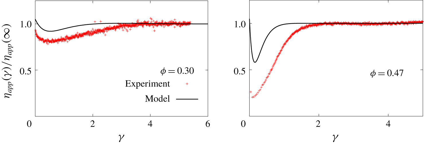
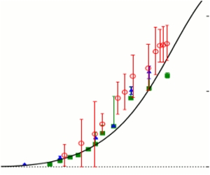
Direct comparisons between model predictions with the constants given in table 1 and the experimental data used for the identification are shown in figures 1–3. Figure 1 shows that predicted steady-state depletion angle and apparent viscosity are indeed in excellent quantitative agreement with the experimental data. Figure 2 presents comparisons for the transient response, namely evolution of apparent viscosity  $\unicode[STIX]{x1D702}_{app}(t)$ versus strain
 $\unicode[STIX]{x1D6FE}(t)=\int _{0}^{t}|\dot{\unicode[STIX]{x1D6FE}}(s)|\text{d}s$ after a shear reversal. Let us recall that the experiments of Blanc et al. (Reference Blanc, Peters and Lemaire2011) were performed at imposed shear stress, while
 $\dot{\unicode[STIX]{x1D6FE}}(t)$ varies. Note that both model predictions and experimental data are normalized by their respective steady-state values
 $\unicode[STIX]{x1D702}_{app}(\infty )$ in the figure. It is observed that, although the model generally tends to underestimate the amplitude of the transient response, a satisfactory qualitative behaviour is nevertheless obtained for all values of
 $\unicode[STIX]{x1D719}$. In particular, the successive phases present in the measurements, namely the initial sharp drop in apparent viscosity, the smooth evolution to a minimum and the relaxation towards the steady state, are all reproduced. The typical duration of the transient phase is also correctly captured.
Evolution of apparent viscosity  $\unicode[STIX]{x1D702}_{app}$ versus shear strain
 $\unicode[STIX]{x1D6FE}$ after shear reversal: comparison between model prediction and experimental measurements of Blanc et al. (Reference Blanc, Peters and Lemaire2011) for two volume fractions
 $\unicode[STIX]{x1D719}$.

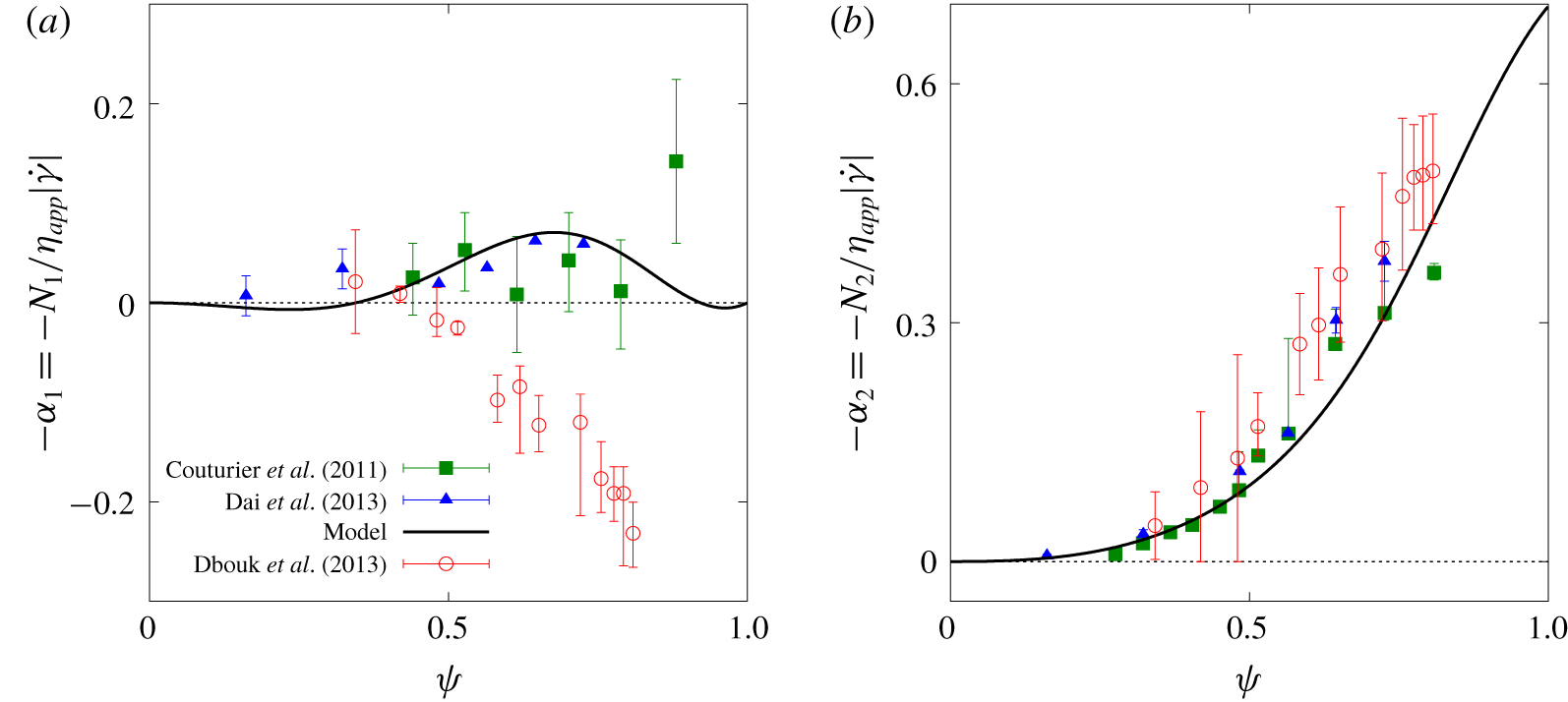
Evolution of steady-state normal stress ratios (a)  $\unicode[STIX]{x1D6FC}_{1}$ and (b)
 $\unicode[STIX]{x1D6FC}_{2}$ versus reduced volume fraction
 $\unicode[STIX]{x1D713}$: comparison between model predictions and experimental measurements of Couturier et al. (Reference Couturier, Boyer, Pouliquen and Guazzelli2011), Dai et al. (Reference Dai, Bertevas, Qi and Tanner2013) and Dbouk et al. (Reference Dbouk, Lobry and Lemaire2013).

Figure 3 presents the evolution of steady-state normal stress ratios  $\unicode[STIX]{x1D6FC}_{1}$ and
 $\unicode[STIX]{x1D6FC}_{2}$ as a function of reduced volume fraction
 $\unicode[STIX]{x1D713}$. The model appears to successfully capture the main features of the normal stress measurements reported in the studies of Couturier et al. (Reference Couturier, Boyer, Pouliquen and Guazzelli2011) and Dai et al. (Reference Dai, Bertevas, Qi and Tanner2013), namely
 $N_{2}<0$ and
 $|N_{1}|<|N_{2}|$. Predictions for the second normal stress ratio
 $\unicode[STIX]{x1D6FC}_{2}$ show a strong monotonic decrease with
 $\unicode[STIX]{x1D713}$, and are in excellent quantitative agreement with the data (figure 3b). Regarding the first normal stress difference, the model predicts non-monotonic variations of the ratio
 $\unicode[STIX]{x1D6FC}_{1}$ with
 $\unicode[STIX]{x1D713}$ (figure 3a). Values of
 $\unicode[STIX]{x1D6FC}_{1}$ are positive but very small for
 $\unicode[STIX]{x1D713}\lesssim 0.4$, negative and decreasing with
 $\unicode[STIX]{x1D713}$ for
 $0.4\lesssim \unicode[STIX]{x1D713}\lesssim 0.7$ and then increasing again towards the concentrated limit
 $\unicode[STIX]{x1D6FC}_{1}(1)=0$ (see § 3.4). Here also, these predictions appear to be in good quantitative agreement with the measurements in terms of overall magnitude, albeit the existence of non-monotonic variations cannot be confirmed from existing data due to the level of experimental noise. For comparison, experimental measurements obtained by Dbouk et al. (Reference Dbouk, Lobry and Lemaire2013) (not used for the adjustment) are also shown in figure 3, using a value
 $\unicode[STIX]{x1D719}_{m}=0.58$ for the volume fraction scaling. These measurements are fully consistent with the two other datasets and the model for
 $\unicode[STIX]{x1D6FC}_{2}$, but show positive values of
 $\unicode[STIX]{x1D6FC}_{1}$, thereby highlighting the need for additional characterizations of the first normal stress difference in these systems.
4.2 Comparison with independent particle pressure measurements
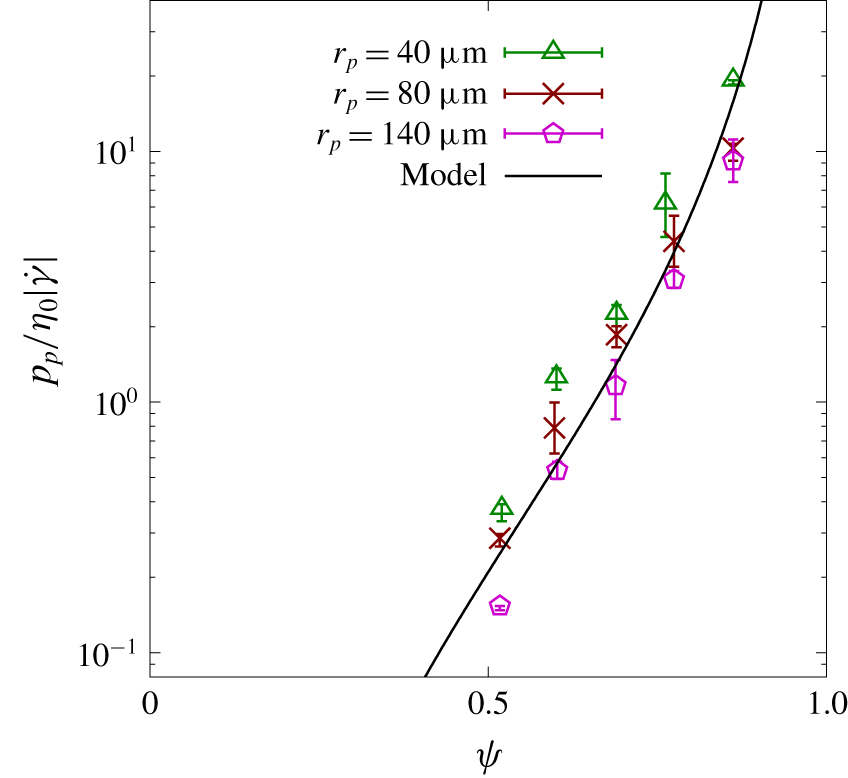
Evolution of steady-state normalized particle pressure  $p_{p}/(\unicode[STIX]{x1D702}_{0}|\dot{\unicode[STIX]{x1D6FE}}|)$ versus reduced volume fraction
 $\unicode[STIX]{x1D713}$: comparison between model predictions and experimental measurements of Deboeuf et al. (Reference Deboeuf, Gauthier, Martin, Yurkovetsky and Morris2009). The consistent data obtained for three different values of particle radius
 $r_{p}$ are shown.

Model predictions were also assessed against steady-state particle pressure measurements obtained by Deboeuf et al. (Reference Deboeuf, Gauthier, Martin, Yurkovetsky and Morris2009). Those authors used a suspending fluid of viscosity  $\unicode[STIX]{x1D702}_{0}=3~\text{Pa}~\text{s}$ and different sets of particles with radii ranging between
 $40$ and
 $140~\unicode[STIX]{x03BC}\text{m}$. As they did not provide the value of maximum volume fraction
 $\unicode[STIX]{x1D719}_{m}$ in their systems, we used
 $\unicode[STIX]{x1D719}_{m}=0.58$ to rescale their data. We emphasize that this new dataset was not used for the identification of model constants. As shown in figure 4, model predictions obtained with the values of constants given in table 1 show here also a good agreement with the experimental measurements. This remarkable result validates the introduction of reduced volume fraction
 $\unicode[STIX]{x1D713}=\unicode[STIX]{x1D719}/\unicode[STIX]{x1D719}_{m}$ in the dependence laws for the material parameters (see § 3.3), and indicates that the model constants involved in these dependence laws can be regarded, at least to a first approximation, as independent of the experimental conditions. In other words, the influence of experimental conditions is fully encoded in the maximum volume fraction
 $\unicode[STIX]{x1D719}_{m}$ used to rescale the volume fraction values.
5 Sensitivity study
A systematic sensitivity study of model predictions with respect to the seven model constants  $a$,
 $b$,
 $\unicode[STIX]{x1D714}$,
 $\bar{\unicode[STIX]{x1D702}}_{e}$,
 $\bar{\unicode[STIX]{x1D6FD}}$,
 $\bar{\unicode[STIX]{x1D6FF}}_{1}$ and
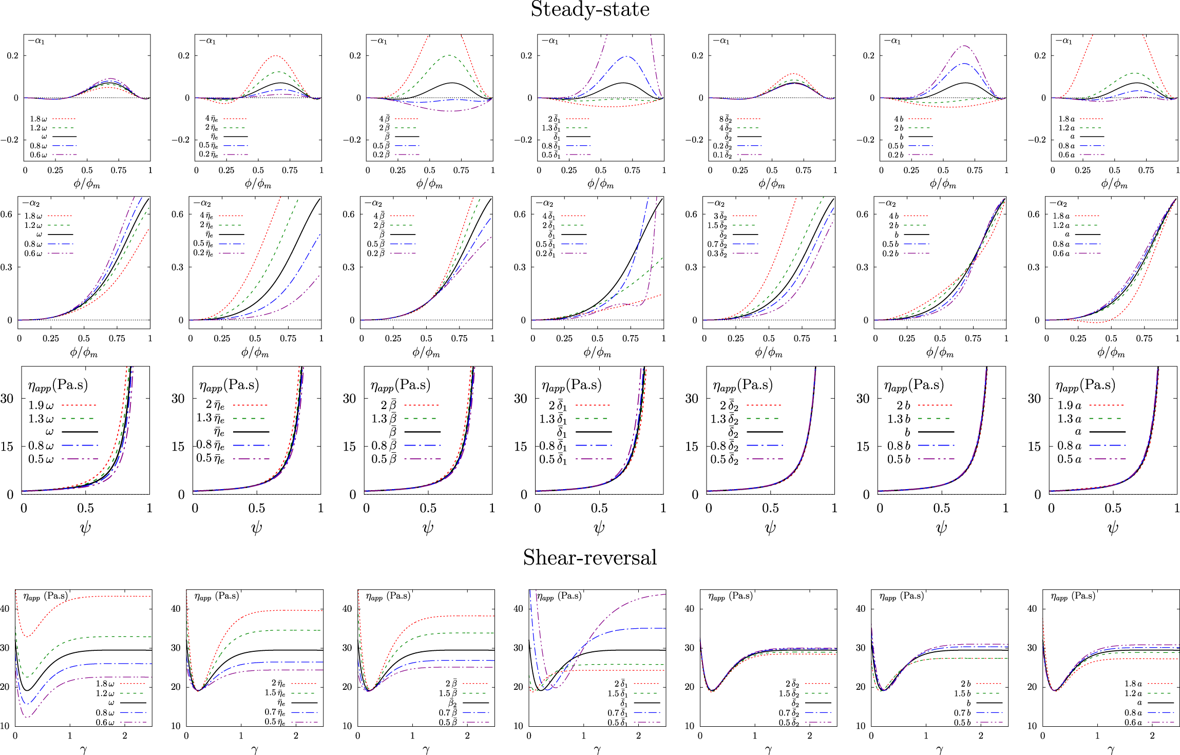
 $\bar{\unicode[STIX]{x1D6FF}}_{2}$ was performed. Figure 5 shows the evolution of steady-state normal stress ratios
 $\unicode[STIX]{x1D6FC}_{1}$ and
 $\unicode[STIX]{x1D6FC}_{2}$ and steady-state apparent viscosity
 $\unicode[STIX]{x1D702}_{app}$ versus
 $\unicode[STIX]{x1D713}$ (upper three rows), as well as the transient evolution of
 $\unicode[STIX]{x1D702}_{app}$ after a shear reversal (lower row), when model constants are varied in consistent
 $[-50\%,+100\%]$ ranges around their reference values obtained through identification (see § 4.1).
Upper three rows: evolution of steady-state normal stress ratios  $\unicode[STIX]{x1D6FC}_{1}$ and
 $\unicode[STIX]{x1D6FC}_{2}$ and apparent viscosity
 $\unicode[STIX]{x1D702}_{app}$ versus reduced volume fraction
 $\unicode[STIX]{x1D713}$ as the seven model constants
 $\unicode[STIX]{x1D714}$,
 $\bar{\unicode[STIX]{x1D702}}_{e}$,
 $\bar{\unicode[STIX]{x1D6FF}}_{1}$,
 $\bar{\unicode[STIX]{x1D6FF}}_{2}$,
 $a$,
 $b$ and
 $\bar{\unicode[STIX]{x1D6FD}}$ vary around their reference values indicated in table 1 (see legends). Lower row: the same for the transient evolution of apparent viscosity
 $\unicode[STIX]{x1D702}_{app}$ after a shear reversal (case
 $\unicode[STIX]{x1D719}=0.44$ and
 $\unicode[STIX]{x1D719}_{m}=0.535$).

It is observed that a variation of any of the model constants implies a significant effect on at least one of the displayed quantities. Hence, none of the terms introduced in the Cauchy stress equation (2.1c) can be omitted without significantly degrading the match with experimental observations. We also note the existence of non-trivial couplings between these different terms, which explains the difficulties encountered in the identification procedure when trying to simultaneously reproduce steady-state and transient experimental data (see § 4.1). Note that unphysical predictions  $|\unicode[STIX]{x1D6FC}_{1}|\geqslant |\unicode[STIX]{x1D6FC}_{2}|$ are obtained when values of
 $\bar{\unicode[STIX]{x1D6FF}}_{1}$ are close to zero, when values of
 $\bar{\unicode[STIX]{x1D6FD}}$ are too high or when
 $a\approx 1$.
A closer look at the results provides insights into the physical interpretation of the different model constants. In steady state, the constant  $\bar{\unicode[STIX]{x1D702}}_{e}$ acts as a magnitude scaling for all stress terms that are non-colinear to the strain rate
 $\dot{\unicode[STIX]{x1D738}}$ (see (3.4)). Accordingly, this affects both normal stress ratios
 $\unicode[STIX]{x1D6FC}_{1}$ and
 $\unicode[STIX]{x1D6FC}_{2}$. Conversely,
 $\bar{\unicode[STIX]{x1D6FD}}$ only acts on terms that are quadratic in
 $\dot{\unicode[STIX]{x1D738}}$, and mostly affects the first normal stress ratio
 $\unicode[STIX]{x1D6FC}_{1}$. Both
 $\bar{\unicode[STIX]{x1D702}}_{e}$ and
 $\bar{\unicode[STIX]{x1D6FD}}$ also play a role in the steady-state viscosity
 $\unicode[STIX]{x1D702}_{app}$, but have essentially no influence on the minimum observed during the transient evolution of
 $\unicode[STIX]{x1D702}_{app}$.
The constant  $\bar{\unicode[STIX]{x1D6FF}}_{1}$ is interpreted as a characteristic strain controlling the length of the transients. In particular, this constant sets the position of the minimum in
 $\unicode[STIX]{x1D702}_{app}$. This constant also plays a strong role in the steady-state values of apparent viscosity and normal stress ratios. This ubiquitous role is consistent with the fact that
 $\unicode[STIX]{x1D6FF}_{1}$ is the only parameter present in both the constitutive equation for
 $\unicode[STIX]{x1D748}$ (2.1c) and the evolution equation for
 $\unicode[STIX]{x1D738}_{e}$ (2.2a).
The constants  $\bar{\unicode[STIX]{x1D6FF}}_{2}$,
 $a$ and
 $b$ do not have much influence on the apparent viscosity
 $\unicode[STIX]{x1D702}_{app}$. The constant
 $\bar{\unicode[STIX]{x1D6FF}}_{2}$ essentially acts on the second normal stress ratio
 $\unicode[STIX]{x1D6FC}_{2}$, while the constants
 $a$ and
 $b$ have a more pronounced effect on
 $\unicode[STIX]{x1D6FC}_{1}$. However, an unphysical change of sign of
 $\unicode[STIX]{x1D6FC}_{2}$ is observed when
 $a\approx 1$. These observations are consistent with equations (3.4).
Finally, the constant  $\unicode[STIX]{x1D714}$ is responsible for an overall shift of the apparent viscosity
 $\unicode[STIX]{x1D702}_{app}$ in both transient and steady-state regimes, but only weakly affects the normal stress ratios
 $\unicode[STIX]{x1D6FC}_{1}$ and
 $\unicode[STIX]{x1D6FC}_{2}$.
6 Discussion and conclusions
An improved, rate-independent rheological model for non-colloidal suspensions of rigid spheres, involving the evolution of a conformation tensor, is presented. The model upgrades that of Ozenda et al. (Reference Ozenda, Saramito and Chambon2018) in several aspects. While the structure of the linear evolution equation (2.1a) for the conformation tensor is unchanged, a more general Gordon–Schowalter tensor derivative is used, with a material parameter  $a\in \! ]0,1\ $N_{1}$ and
 $N_{2}$ in steady state. Although the contributions of the different terms to the overall rheological behaviour of the suspension appear to be strongly coupled, a systematic sensitivity study was performed to provide insights into the physical interpretation of the different model parameters. Note, however, that the sensitivity study was performed for limited ranges of the parameters, and thus might not be representative of the model behaviour when parameters are varied in much larger ranges.
The model was compared to different experimental datasets involving various suspending fluids and particle sizes. To that aim, the material parameters were all expressed in terms of reduced volume fraction  $\unicode[STIX]{x1D713}=\unicode[STIX]{x1D719}/\unicode[STIX]{x1D719}_{m}$, where the maximum volume fraction
 $\unicode[STIX]{x1D719}_{m}$ varies among the experiments, and a of set of seven model constants. The good agreement observed with steady-state data, in terms of apparent viscosity, normal stress differences and particle pressure, suggests that the rheological model, together with the constants given in table 1, can be applied to large range of non-colloidal suspensions. Regarding the transient responses, only qualitative agreement was obtained with experimental data.
Further improvements of these transient predictions would certainly require complementing our minimal model with additional terms, for instance polynomial dependences of the material parameters upon the invariants of the texture tensor (Hand Reference Hand1962), or introduction of additional microstructural tensorial variables (Goddard Reference Goddard2006). Along the same line, introduction of a plasticity term in the constitutive law would open interesting perspectives for tackling highly concentrated regimes close to, or above, the jamming transition, in which the rheological behaviour becomes dominated by sustained granular contacts (Pailha & Pouliquen Reference Pailha and Pouliquen2009; Baumgarten & Kamrin Reference Baumgarten and Kamrin2019).
The capability of the presented model to predict accurate normal stress differences in steady state potentially opens the way to computations of elongational or more complex flows. Such applications to a larger class of flows, together with a more systematic parameter identification procedure, would also make it possible to improve the physical interpretation of the different terms introduced in the expression of the Cauchy stress tensor. Here also, detailed comparisons with experiments (e.g. Dai & Tanner Reference Dai and Tanner2017) will, however, be necessary to assess the validity of the model, and particularly of the dependences of material parameters upon volume fraction introduced in § 3.3, beyond the simple shear configuration investigated in this study. A more in-depth analysis of the mathematical and thermodynamical properties of the model would also need to be undertaken. The new rheological model could also be coupled to an evolution equation for the volume fraction in order to address particle migration processes (e.g. Miller & Morris Reference Miller and Morris2006; Haddadi et al. Reference Haddadi, Shojaei-Zadeh, Connington and Morris2014), test the effect of normal stress differences over longer time scales and allow for comparisons with other modelling approaches (e.g. Dbouk Reference Dbouk2016).
Finally, let us also note that, although the focus of the present paper was mainly on trying to reproduce physical experiments, systematic comparisons with discrete simulation results (e.g. Chacko et al. Reference Chacko, Mari, Fielding and Cates2018; Singh et al. Reference Singh, Mari, Denn and Morris2018) could constitute a fruitful avenue for further validating and improving our rheological model. In particular, comparisons regarding the evolution of normal stress differences during transients, for which no experimental data are currently available, could provide useful additional insights.
Declaration of interests
The authors report no conflict of interest.
Appendix A. Eigen directions of $\unicode[STIX]{x1D738}_{e}$

We prove here that, in stationary simple shear flow, the depletion angle, i.e. the angle between the  $x$ axis and the direction of the eigenvector associated with the largest eigenvalue of
 $\unicode[STIX]{x1D738}_{e}$, is expressed as
 $$\begin{eqnarray}\unicode[STIX]{x1D6FF}_{1}=\tan (2\unicode[STIX]{x1D703}_{e}).\end{eqnarray}$$
From (3.3a) to (3.3c), eigenvalues of  $\unicode[STIX]{x1D738}_{e}$, denoted as
 $\unicode[STIX]{x1D706}_{min}\leqslant \unicode[STIX]{x1D706}_{max}$, are both non-zero and are written
 $$\begin{eqnarray}\displaystyle & \displaystyle \unicode[STIX]{x1D706}_{min}={\displaystyle \frac{\unicode[STIX]{x1D6FF}_{1}^{-1}}{1+\unicode[STIX]{x1D6FF}_{1}^{-2}(1-a^{2})}}(a\unicode[STIX]{x1D6FF}_{1}^{-1}-(\unicode[STIX]{x1D6FF}_{1}^{-2}+1)^{1/2}), & \displaystyle \nonumber\\ \displaystyle & \displaystyle \unicode[STIX]{x1D706}_{max}={\displaystyle \frac{\unicode[STIX]{x1D6FF}_{1}^{-1}}{1+\unicode[STIX]{x1D6FF}_{1}^{-2}(1-a^{2})}}(a\unicode[STIX]{x1D6FF}_{1}^{-1}+(\unicode[STIX]{x1D6FF}_{1}^{-2}+1)^{1/2}). & \displaystyle \nonumber\end{eqnarray}$$
The corresponding eigenvectors are
 $$\begin{eqnarray}\boldsymbol{v}_{min}=\left[\begin{array}{@{}c@{}}\unicode[STIX]{x1D6FF}_{1}^{-1}-(\unicode[STIX]{x1D6FF}_{1}^{-2}+1)^{1/2}\\ 1\end{array}\right],\quad \boldsymbol{v}_{max}=\left[\begin{array}{@{}c@{}}1\\ (\unicode[STIX]{x1D6FF}_{1}^{-2}+1)^{1/2}-\unicode[STIX]{x1D6FF}_{1}^{-1}\end{array}\right].\end{eqnarray}$$
Accordingly, we obtain
 $$\begin{eqnarray}\unicode[STIX]{x1D703}_{e}=\text{atan}((\unicode[STIX]{x1D6FF}_{1}^{-2}+1)^{1/2}-\unicode[STIX]{x1D6FF}_{1}^{-1})={\displaystyle \frac{\text{atan}(\unicode[STIX]{x1D6FF}_{1})}{2}},\end{eqnarray}$$
which is equivalent to (A 1). Observe that  $\forall ~\unicode[STIX]{x1D6FF}_{1}>0,~\unicode[STIX]{x1D703}_{e}\in \! ]0,\unicode[STIX]{x03C0}/4\ $\unicode[STIX]{x1D738}_{e}$ depend on the parameter
 $a$ of the tensor derivative, the eigenvectors are independent thereof. Hence, all the relations between microstructure orientation and model parameters derived in Ozenda et al. (Reference Ozenda, Saramito and Chambon2018), notably (A 1), remain unchanged in the present model.
Appendix B. Identification of model constants
The rheological model proposed in this paper involves seven constants to be identified:  $a$,
 $b$,
 $\unicode[STIX]{x1D714}$,
 $\bar{\unicode[STIX]{x1D702}}_{e}$,
 $\bar{\unicode[STIX]{x1D6FD}}$,
 $\bar{\unicode[STIX]{x1D6FF}}_{1}$ and
 $\bar{\unicode[STIX]{x1D6FF}}_{2}$. Global identification of these parameters with respect to experimental data was achieved by minimizing the following cost function:
 $$\begin{eqnarray}\displaystyle J & = & \displaystyle {\displaystyle \frac{w_{a}}{\unicode[STIX]{x1D713}_{2}-\unicode[STIX]{x1D713}_{1}}}\int _{\unicode[STIX]{x1D713}_{1}}^{\unicode[STIX]{x1D713}_{2}}|\unicode[STIX]{x1D703}_{e}(\unicode[STIX]{x1D713})-\unicode[STIX]{x1D703}_{e}^{obs}(\unicode[STIX]{x1D713})|^{2}\,\text{d}\unicode[STIX]{x1D713}+{\displaystyle \frac{w_{v}}{\unicode[STIX]{x1D713}_{4}-\unicode[STIX]{x1D713}_{3}}}\int _{\unicode[STIX]{x1D713}_{3}}^{\unicode[STIX]{x1D713}_{4}}|\unicode[STIX]{x1D702}_{app}(\unicode[STIX]{x1D713})-\unicode[STIX]{x1D702}_{app}^{obs}(\unicode[STIX]{x1D713})|^{2}\,\text{d}\unicode[STIX]{x1D713}\nonumber\\ \displaystyle & & \displaystyle +\,\mathop{\sum }_{i=1}^{2}{\displaystyle \frac{w_{s,i}}{\unicode[STIX]{x1D713}_{m}}}\int _{0}^{\unicode[STIX]{x1D713}_{m}}|\unicode[STIX]{x1D6FC}_{i}(\unicode[STIX]{x1D713})-\unicode[STIX]{x1D6FC}_{i}^{obs}(\unicode[STIX]{x1D713})|^{2}\,\text{d}\unicode[STIX]{x1D713}\nonumber\\ \displaystyle & & \displaystyle +\,\mathop{\sum }_{k=1}^{5}{\displaystyle \frac{w_{t,k}}{\unicode[STIX]{x1D6FE}_{k}}}\int _{0}^{\unicode[STIX]{x1D6FE}_{k}}|\unicode[STIX]{x1D702}_{app}(\unicode[STIX]{x1D713}_{k},\unicode[STIX]{x1D6FE})-\unicode[STIX]{x1D702}_{app,k}^{obs}(\unicode[STIX]{x1D6FE})|^{2}\,\text{d}\unicode[STIX]{x1D6FE}.\nonumber\end{eqnarray}$$
The function  $\unicode[STIX]{x1D703}_{e}^{obs}(\unicode[STIX]{x1D713})$ is a piecewise-constant interpolation of steady-state depletion angle measurements reported by Blanc et al. (Reference Blanc, Lemaire, Meunier and Peters2013) for
 $\unicode[STIX]{x1D713}\in [\unicode[STIX]{x1D713}_{1},\unicode[STIX]{x1D713}_{2}]$, with
 $\unicode[STIX]{x1D713}_{1}=0.088$ and
 $\unicode[STIX]{x1D713}_{2}=0.98$ the range of reduced volume fraction explored in the experiments.
The function  $\unicode[STIX]{x1D702}_{app}^{obs}(\unicode[STIX]{x1D713})$ is a piecewise-constant interpolation of steady-state values of apparent viscosity measured by Blanc et al. (Reference Blanc, Peters and Lemaire2011) for
 $\unicode[STIX]{x1D713}\in [\unicode[STIX]{x1D713}_{3},\unicode[STIX]{x1D713}_{4}]$, with
 $\unicode[STIX]{x1D713}_{3}=0.56$ and
 $\unicode[STIX]{x1D713}_{4}=0.93$ in this case. The functions
 $\unicode[STIX]{x1D6FC}_{1}^{obs}(\unicode[STIX]{x1D713})$ and
 $\unicode[STIX]{x1D6FC}_{2}^{obs}(\unicode[STIX]{x1D713})$ are piecewise-constant interpolations of steady-state values of normal stress ratios measured by Couturier et al. (Reference Couturier, Boyer, Pouliquen and Guazzelli2011) and Dai et al. (Reference Dai, Bertevas, Qi and Tanner2013) for
 $\unicode[STIX]{x1D713}\in [0,\unicode[STIX]{x1D713}_{m}]$, with
 $\unicode[STIX]{x1D713}_{m}=0.81$ the maximal reduced volume fraction reached in the experiments. The functions
 $\unicode[STIX]{x1D702}_{app,k}^{obs}(\unicode[STIX]{x1D6FE})$,
 $k=1\ldots 5$, represent the transient evolutions of apparent viscosity during the five shear-reversal experiments of Blanc et al. (Reference Blanc, Peters and Lemaire2011) characterized by reduced volume fractions
 $\unicode[STIX]{x1D713}_{k}$. Here,
 $\unicode[STIX]{x1D6FE}_{k}$,
 $k=1\ldots 5$, represent the maximal strain reached in each experiment. Lastly, the function
 $\unicode[STIX]{x1D702}_{app}(\unicode[STIX]{x1D713},\unicode[STIX]{x1D6FE})$ is associated with the transient solution of the model, while the functions
 $\unicode[STIX]{x1D703}_{e}(\unicode[STIX]{x1D713})$,
 $\unicode[STIX]{x1D702}_{app}(\unicode[STIX]{x1D713})$,
 $\unicode[STIX]{x1D6FC}_{1}(\unicode[STIX]{x1D713})$ and
 $\unicode[STIX]{x1D6FC}_{2}(\unicode[STIX]{x1D713})$ are associated with the steady-state solution. The factors
 $w_{a}$,
 $w_{e}$,
 $w_{s,i}$ and
 $w_{t,k}$ are the relative weights of the different terms of the cost function
 $J$.
The minimization problem of  $J$ was solved with a Levenberg–Marquardt method (More, Garbow & Hillstrom Reference More, Garbow and Hillstrom1980), using the optimization library lmfit (Newville et al. Reference Newville, Stensitzki, Allen, Rawlik, Ingargiola and Nelson2016). As explained in § 4.1, larger values had to be used for the weights
 $w_{a}$,
 $w_{e}$ and
 $w_{s,i}$, with respect to
 $w_{t,k}$, in order to promote the agreement with steady-state measurements. In addition, after the global identification step, a secondary, one-by-one, adjustment of each model constant was performed in order to further improve the solution. Final values of identified model constants are indicated in table 1.